Embed Size (px)
Citation preview

Development of a Freight Policy Analysis Tool for Northeastern Illinois and the United States
Freight Activity Microsimulation Estimator
Kazuya Kawamura (PI) Abolfazl (Kouros) Mohammadian
Ammir Samimi Zahra Pourabdollahi Meredith Klekotka
Urban Transportation Center The University of Illinois at Chicago
December 2011

December 10, 2011
2
DISCLAIMER NOTICE
This document is disseminated under the sponsorship of the United States Department of Transportation (USDOT) and the Illinois Department of Transportation (IDOT) in the interest of information exchange. The United States Government and the Illinois Department of Transportation assume no liability for its contents or use thereof.
The United States Government and the Illinois Department of Transportation do not endorse manufacturers’ products. Trademarks or manufacturers’ names appear in the document only because they are essential to this report’s objectives.
This report’s contents reflect the views of the authors, who are responsible for the facts and the accuracy of the data presented herein. The contents do not necessarily reflect the official views or policies of the USDOT or IDOT.
December 10, 2011
3
Table of Contents CHAPTER PAGE
Chapter 1. Introduction ...................................................................................................... 6
1.1. Background .............................................................................................................. 6
1.2. Scope ........................................................................................................................ 7
1.3. Data .......................................................................................................................... 8
Chapter 2. Literature Review ............................................................................................ 10
2.1. Research Need ........................................................................................................ 10
2.2. Freight Demand Models ........................................................................................ 12
2.2.1. Aggregate Models............................................................................................ 13
2.2.1. Disaggregate Models ....................................................................................... 15
2.2.2. Freight Mode Choice Models .......................................................................... 17
2.3. Freight Microsimulation Efforts............................................................................. 17
Chapter 3. Model Framework ........................................................................................... 22
3.1 Overview ................................................................................................................. 22
3.2 Model Assumptions................................................................................................. 25
3.3. Data ........................................................................................................................ 25
3.3.1. Information on Business Establishments ........................................................ 28
3.3.2. Aggregate Freight Movements ....................................................................... 30
3.4. Information on Individual Shipments and Supply Chains ..................................... 35
3.5. Transportation Network Specifications .................................................................. 35
Chapter 4. Model Estimation ............................................................................................ 37
4.1. Firm-types Generation............................................................................................ 37
4.2. Supply Chain Replication....................................................................................... 37

December 10, 2011
4
4.2.1. Generation of Candidate Suppliers .................................................................. 38
4.2.2. Evaluation of Candidate Suppliers .................................................................. 39
4.3. Shipment Size Determination ................................................................................ 39
4.4. Mode Choice Model .............................................................................................. 40
4.4.1. Explanatory Model .......................................................................................... 42
4.4.2.Parsimonious Model ......................................................................................... 43
Chapter 5. Model Implementation and Validation ........................................................... 48
5.1. Firm-types Generation............................................................................................ 48
5.2. Supply Chain Replication....................................................................................... 49
5.3. Shipment Size Determination ................................................................................ 50
5.4. Mode Split .............................................................................................................. 53
5.5. Validation ............................................................................................................... 55
Chapter 6. Conclusion ....................................................................................................... 57 Cited literature .................................................................................................................. 60 Appendix A. FUZZY EXPERT SYSTEM FOR Supplier Selection Model .................... 71
1. Fuzzy variables .......................................................................................................... 71
2. Fuzzification method ................................................................................................. 72
3. Inference method ....................................................................................................... 74
4. Defuzzification method ............................................................................................. 76
Appendix B. Shipment Size Model .................................................................................. 77
1. Initialization .............................................................................................................. 77
2. Modified Iterative Proportional Fitting (IPF)............................................................ 78
Appendix C. UIC National Freight Survey....................................................................... 80
1. Survey Development ................................................................................................ 80

December 10, 2011
5
2. Descriptive Statistics ................................................................................................ 83
3. Lessons Learned ....................................................................................................... 86
4. Non-Response Bias Analysis ................................................................................... 86

December 10, 2011
6
CHAPTER 1. INTRODUCTION
1.1. BACKGROUND
Freight flow volume within the United States has almost doubled over the past
thirty years (Transportation Research Board, 2008). In 2007, over 12 billion tons of
goods, valued at more than $11.6 trillion, were transported in America (Bureau of
Transportation Statistics, 2009). Population growth, economic growth, the proliferation
of e-commerce, and a greater dependence on transportation in the production process
have driven this growth in freight volumes, especially for long-haul and international
shipments (Southworth, 2003). As a national rail hub, metropolitan Chicago is sensitive
to these changes in freight volumes.
Industry sectors, international trade networks, public agencies, and other policy
makers need accurate information about national freight movements to continue
efficiently delivering various goods within and among consumer markets,. They need to
plan for future freight traffic impacts and evaluate the effectiveness of policies and
projects designed to alleviate freight congestion problems.
New federal regulations mandate that state departments of transportation and
metropolitan planning organizations consider these rail freight congestion problems
during the long-range transportation planning process (Transportation Research Board,
2008). Bryan et al. (2007) and many others have argued that transportation planners
should consider rail freight transportation’s environmental, maintenance, and security
costs as well as congestion costs to better formulate practical solutions to freight
congestion problems.
The freight shipment decision-making process is becoming even more complex as
businesses increasingly adopt sophisticated supply chain management strategies and as
the demand for more accurate freight modeling and forecasting tools is growing.

December 10, 2011
7
To help address these needs, a research study team from the University of
Illinois at Chicago has developed a forecasting tool that accurately reflects current freight
flows, incorporates freight operators’ complex modal-choice decisions, and estimates
changes in freight movement based on a variety of variables. Creating a satisfactory
freight model which reflects modal share decisions and facilitates decision making is
challenging. Major research efforts in travel demand modeling have mainly concentrated
on passenger transportation. A state-of-the-art, behavioral freight model is therefore far
behind advancements in ground passenger transportation (Pendyala et al., 2000). The
complex decision-making process, the lack of an acceptable freight modeling framework,
and freight data scarcity are major obstacles that may have prevented freight modeling’s
advancement. This report summarizes the results of the Freight Activity Microsimulation
Estimator study for which the research team developed a state-of-the-art, freight policy
analysis tool for Northeastern Illinois and the United States.
1.2. SCOPE
This study introduces a nationwide behavioral microsimulation framework that
has five basic modules. The first module uses agent-based modeling to replicate firms’
characteristics to organize these firms according to industry type. The second module
uses a fuzzy rule based model to determine the volume and type of commodity flows and
replicates the supply chain design. This model is used because disaggregate data on
supplier selection within the supply chain is lacking. By effectively incorporating
decision making agents into the model, the results are more realistic since they are based
on firms’ behaviors. Incorporating firms’ behavior in the freight transportation model is
the essence of disaggregate freight models. A few researchers have emphasized it
(RAND Europe, 2004; de Jong and Ben-Akiva, 2007; Hensher and Figliozzi, 2007).
In the third module, the study team nationally applied this framework’s open
structure under multiple scenarios to develop a comprehensive freight traffic study that
incorporates freight firms’ complex-decision-making about modal split and the influences

December 10, 2011
8
of supply-chain demands that affect freight flows. The study team has therefore tried to
fill the modeling gap in large scale freight microsimulation and has sought to promote
future behavioral freight microsimulation efforts.
This report details the Freight Activity Microsimulation Estimator framework’s
development and documents the study team’s results in determining national freight
flows along the transportation network. The first application of the five Freight Activity
Microsimulation Estimator modules used the County Business Pattern and Freight
Analysis Framework from 2002 to analyze how freight mode choices affected the
transportation network under a variety of factors.
The second application of the Freight Activity Microsimulation Estimator
framework used the updated 2007 County Business Pattern and Freight Analysis
Framework data sets and incorporated new infrastructure developments affecting freight
flows nationally. This model covers the entire U.S. since freight policies and plans for
Northeastern Illinois cannot be analyzed in isolation from national and even global trends
and major projects planned elsewhere in the country, given Chicago’s role as North
America’s major freight hub.
1.3. DATA
Data scarcity is a major issue that hinders the development of behavioral freight
modeling. Aggregate data, often at the state or urban area level, are usually available but
are insufficient for behavioral freight modeling efforts that need to capture decision-
making processes and interactions at the firm level. This is the primary factor that
hinders the development of freight studies at the disaggregate level (Kumar and
Kockelman, 2008). Surveying freight firms is one option for collecting disaggregate
data, but many decision-makers are unwilling to participate in surveys inquiring about
their shipping decisions, since such information is an important part of their business
strategies. They understandably fear that disclosing their strategies will jeopardize their
competitive edge. Furthermore, knowledgeable persons who can provide input to such

December 10, 2011
9
surveys tend to have a high value of time. This could not only seriously decrease the
response rate and thereby endanger the survey’s credibility, but also make such surveys
very expensive in many cases, even if successful.
This study’s data takes advantage of publicly available U.S. freight and business
data, the Freight Analysis Framework, and County Business Pattern data and incorporates
it with data from a nationwide survey of freight shippers that the University of Illinois at
Chicago previously collected. The diversity of this data is sufficient to produce results
indicating modal choice decisions and the distribution pattern of national freight
movements. However, the highly aggregate nature of the Freight Analysis Framework
data means that the results are susceptible to uncertainty. This model should therefore be
considered as an exploratory effort that will need further improvements.

December 10, 2011
10
CHAPTER 2. LITERATURE REVIEW
This chapter provides a context for this study within the current modeling
frameworks. It contains an overview of past freight demand forecasting efforts,
consisting of aggregate models, disaggregate models, and freight mode choice models.
Freight microsimulation efforts, however, are discussed in another chapter.
2.1. RESEARCH NEED
Supply chain management seeks to satisfy customers as a way to improve
industrial competitiveness and profitability (Stadtler, 2005). Freight industry
deregulation in the early 1980s, increasing globalization, and the use of information
technology prompted freight industries to apply supply chain management (Rodrigue,
2006). This application of supply chain management has led to more efficient and
complex behaviors in commodity production and distribution cycles. Following freight
industry deregulation in the U.S, the logistics-related component’s share of the GDP
decreased from approximately 17% in 1980 to just above 10% in 2000 (AASHTO, 2003).
Long haul commodity flows increased when these firms sought better national or
international partners to form the best possible chains. To survive in such a competitive
market, these firms also had to use logistics professionals to keep transportation costs as
low as possible.
The way that logistics decisions are made within production cycles influences the
transportation costs for raw materials and semi-finished goods. Firms could similarly
optimize the distribution costs for finished goods within a well-organized distribution
system. This could lower the overall costs of goods from the producers to the consumers,
causing a decrease in retail store prices (Rodrigue, 2006).
Hensher and Figliozzi (2007) argued that rapid changes in supply chain structures,
logistics and technological advancements, and freight systems are the primary causes of
the current freight models and policy making tools’ obsolescence. They and many other

December 10, 2011
11
researchers strongly believe that the conventional four-step approach, primarily designed
for passenger transport modeling, cannot adequately capture the complexity of the
international, national, and urban freight movements.
Like the passenger travel demand models, Hensher and Figliozzi’s framework has
four sequential modules: commercial trip generation, distribution, mode choice, and
traffic assignment. However, this framework does not capture strategic decisions that
individual firms make regarding their supply chain designs and operations, such as how
shipping decisions are made, whether to contract out shipping tasks, and whether
consolidation and/or distribution centers are needed.
Southworth (2003) argued that a successful freight forecasting tool must be able
to incorporate rapid changes in supply chain logistics into the planning procedure, either
by adopting traditional methodologies or introducing entirely new frameworks of freight
demand forecasting tools.
Taylor (2001) highlighted the growing trend toward new delivery methods that
used the intermodal transport system’s uncovered capacities to place a premium on transit
time and reliability. One example is just-in-time (JIT) delivery, a cornerstone of
contemporary customer-order-driven markets (Hensher and Figliozzi, 2007).
As goods transportation becomes ever more complex and sophisticated, many
shippers have resorted to outsourcing all or many of their supply chain functions to third-
party logistics companies, or third-party logistics companies. Southworth (2003) has
argued that third-party logistics companies and IT-based logistics service providers are
moving toward more integration and globalization by linking different firms’ logistics
management. This makes predicting shipping decision behaviors even more complicated.
Gray (1982) reviewed behavioral models and highlighted the importance of
identifying decision makers in freight demand modeling procedures. Even in passenger
transportation modeling, the effectiveness of the four-step framework is questioned
(McNally and Recker, 1986).

December 10, 2011
12
In the last few decades, researchers have developed and advanced the Activity
Based Modeling approach (Ettema and Timmermans, 1997). In this emerging
framework, the model includes how individuals (or households) are making decisions
regarding activity type, destination choice, mode choice, etc. The need to incorporate
changes in travel behavior, such as trip chaining, partly motivated this approach.
A limited number of studies have tried to apply the activity-based approach to
freight transportation modeling, but most have not produced satisfactory results given the
lack of data (Hensher and Figliozzi, 2007). In a comparison with the passenger activity-
based modeling approach, Liedtke and Schepperle (2004) argued that commodity
transport modeling’s current state-of-the-practice lacks actor-based microsimulation.
Although there are well-developed standard techniques to model passenger
transportation systems, less attention has been paid to freight demand modeling.
Accordingly, there are much fewer achievements in this area.
The freight transportation decision-making process is extremely difficult to
reproduce. However, freight modelers have made some strides using an agent-based
approach. Behavioral freight demand modeling frameworks are at their early
development stages and establishing a practical and theoretically sound method is yet to
come.
2.2. FREIGHT DEMAND MODELS
The four-step freight modeling framework consists of four sequential modules
and is the primary approach for freight demand forecasting in practice, especially for
metropolitan and statewide planning agencies (Southworth, 2003, Cambridge
Systematics, 1995).
A commonly used criteria for categorizing modeling efforts is vehicle-based
versus commodity-based models. In commodity-based models, modelers estimate
commodity tonnage and convert it into truck trips. They apply payload cost estimates to

December 10, 2011
13
aggregate commodity tonnage and obtain truck trips rates (Fisher and Han, 2001).
Although it lacks consensus on using vehicle versus commodity based models,
vehicle based models dominate freight research (Luk and Chen, 1997). Holguin-Veras
and Thorson (2000), however, argued that both commodity-based and vehicle-based
approaches lead to conceptual inconsistencies since commodity flows should represent
actual freight demand and vehicles should represent logistics decisions.
Winston (1983) also classified the freight models into aggregate and disaggregate
approaches based on the types of data used. This categorization method seems suitable
for this study’s purposes since the study team is focusing on behavioral freight models.
The study team will review aggregate and disaggregate approaches to freight
modeling and provide an overview of existing research on mode-choice models and
microsimulation of freight activity in the following sections.
2.2.1. Aggregate Models
Aggregate models are still the state-of-the-practice in freight transport modeling
(Liedtke and Schepperle, 2004). They predominate modeling because they require
simple data compared to the disaggregate approach and rely on historical trends
(Pendyala et al., 2000). Although many practitioners and decision-makers are aware of
the aggregate models’ drawbacks, they face pressure to keep data collection costs low
and must compromise between modeling quality and project expenses.
The application of the four-step modeling framework is typically aggregate in
nature. Generation and attraction of commercial trips are usually based on zonal
economic activity or employment (Anderson et al., 2007). Although information on an
industry’s economic activity is difficult to obtain, there are some publications that
provide an average rate of commercial trip generation and attraction for freight planners
(Fischer and Han, 2001).
The distribution of commercial trips is commonly carried out by a gravity model
with shipping distance as the impedance (Auld, 2007).

December 10, 2011
14
Southworth (2003) discussed different approaches for commercial trip
distribution, including the spatial interaction method. Mode choice is a critical
component of the framework. Modelers previously estimated mode choice based on
shipping costs (Cunningham, 1982).
Many four step models have now attempted to incorporate both commodity and
vehicle trips by adding a fifth step that converts the commodity flow into vehicle flow,
before assigning traffic (Fischer et al., 2000). Modelers, however, usually assign urban
freight traffic to the cheapest or quickest path with base traffic when converting it to a
passenger vehicle equivalent. This trend of not considering modal split is very common
in aggregate four-step approaches and is rooted to the aggregate nature of the data that is
not able to capture the behavioral complexities of modal selection decisions.
Tavasszy et al. (1998) were pioneers in considering logistics decisions in freight
transportation planning. They developed the Strategic Model for Integrated Logistic
Evaluations in the Netherlands for the Dutch Ministry of Transport, Public Works, and
Water Management. The Strategic Model for Integrated Logistic Evaluations is an
aggregate model (Yang et al., 2009), yet containing some disaggregate logistics
components.
More details on four-step freight demand modeling is provided in the Quick
Response Freight Manual (Cambridge Systematics, 1997) for the U.S. Department of
Transportation. National Cooperative Highway Research Project (NCHRP) Report 606,
Yang et al. (2009), and Pendyala et al. (2000), also provided valuable reviews of similar
past practices. The American Association of State Highway and Transportation Officials
(AASHTO) in cooperation with the Federal Highway Administration (Transportation
Research Board, 2008) sponsored a recent study that is a comprehensive source for
freight demand models in the U.S.

December 10, 2011
15
2.2.1. Disaggregate Models
This section provides a short review of some disaggregate modeling efforts in
previous freight demand studies. Although disaggregate models are more appealing and
considered theoretically sounder, the limited availability of disaggregate data often
prevents development and implementation of these models. Nevertheless, a considerable
number of disaggregate models have focused on urban freight movement and modal
selection, and recently on supply chain and logistic decisions.
Regan and Garrido (2001) pointed out several general drawbacks of aggregate
models and discussed behavioral and inventory disaggregate freight models. Behavioral
disaggregate freight models strive to capture the utility maximization process for certain
decision-makers. Inventory disaggregate freight models, however, attempt to model
firms' production and logistic decisions based on economic optimization.
Pendyala et al. (2000) argued that approximations are unavoidable in developing
logistics cost functions for practical inventory models.
Inventory disaggregate freight models treat production-related variables, such as
shipment size, endogenously with mode choice decisions (Pendyala et al., 2000). They
argued that some approximations in these models could make them very similar to
behavioral disaggregate freight models.
Baumol and Vinod (1970) are among the pioneers in modeling both mode choice
and demands for links on a freight network. They used the same approach that had been
developed for the analysis of passenger transportation. Their mode choice model
considers the trade-off between transportation cost, time, reliability, and safety. It also
accounts for carrier and commodity heterogeneity.
Harker and Friesz (1986) also applied the conventional four-step approach with
substantial modifications to the supply and demand models.
Hunt and Stefan (2007) developed a behavioral urban freight model, capable of
predicting commercial vehicle movements under different policy scenarios. This model
December 10, 2011
16
shed light on some urban freight movements, including the treatment of empty trips, less
than truck load movements, shipment allocation to vehicles, and conversion of
commodity flows to shipments. It also integrated an aggregate passenger travel
component to account for the interdependencies of urban freight movement and
passenger transportation.
Recently, there has been a growing interest in supply chain and logistics
modeling. Some of these models were developed for urban freight studies. Fischer et al.
(2005) and Yang et al. (2009) provided summaries of recent developments in supply
chain models. Tavasszy et al. (1998) is a prominent example of supply chain and
logistics modeling efforts. They developed a series of disaggregate logistics models,
called the Strategic Model for Integrated Logistics Evaluations, together with an
economic input-output model to provide a decision tool for policy evaluation for the
Netherlands. Also, Boerkamps et al. (2000) developed an urban supply chain model,
called GoodTrip, for the city of Groningen in the Netherlands. The GoodTrip is a
disaggregate model that defines supply chain patterns and urban truck tours to provide
insights into how logistics decisions affect urban truck traffic. De Jong and Ben-Akiva
(2007) also embarked upon the development of a logistics module to be included in the
existing freight demand model for Norway and Sweden.
Behavioral freight models are extremely scarce in the literature and a limited
number of such studies are found among recent works. Companies have become
increasingly customer-order-driven and new production systems such as Just-in-Time
(JIT) are now common. De Jong and Ben-Akiva (2007) stated that almost all the existing
freight transportation studies are missing supply chain and logistics components. They
introduced some behavioral models that incorporated firms’ characteristics, which were a
substantial step toward establishing a feasible framework for a behavioral freight model.
Hensher and Figliozzi (2007) highlighted the importance of disaggregate
behavioral freight models in mitigating traffic congestion and maintaining the freight
transportation system’s efficiency and reliability. Holguin-Veras (2000) also discussed

December 10, 2011
17
an urban freight modeling framework capable of incorporating logistics information and
trip chaining behaviors.
2.2.2. Freight Mode Choice Models
Mode choice is one of the most critical parts of any freight demand modeling
framework, and Freight Activity Microsimulation Estimator is no exception. The amount
of literature on this issue is surprisingly modest mainly given the absence of suitable data
to estimate such models. A direct comparison of shipment costs was the primary method
in the earliest freight mode choice models (Cunningham, 1982).
Reliability, flexibility, safety, and some other non-cost factors entered the analysis
when the random utility models emerged ( Norojono and Young, 2003). Random utility
models become outdated, however, when supply chain concepts required the
development of actor-based models that incorporated the role of actual decision-makers
in freight movement determination. Many companies adopted new supply chain
concepts, which have influenced shipping preferences (Hensher and Figliozzi, 2007) and
therefore require a fundamental revision of the existing approach to freight demand
modeling.
Freight mode choice models vary greatly in scope and design. Whether logit
versus probit or aggregate versus disaggregate, each model calibrates the impact of
various factors on freight firms’ mode choice decisions
Based on a review of these studies, the dominant factors impacting freight mode
choice in the literature can be summarized as: accessibility, reliability, cost, time,
flexibility, and past experience with each mode.
2.3. FREIGHT MICROSIMULATION EFFORTS
Many previous studies have called for a behavioral freight microsimulation
model. Liedtke and Schepperle (2004) argued that freight transportation modeling

December 10, 2011
18
literature lacks appropriate “actor-based” micro-level models. Actual decision-makers’
roles are therefore mostly overlooked.
Many other studies have emphasized the need for a better understanding of
decision-making procedures including Gray (1982), Southworth (2003), Wisetjindawat et
al. (2005), de Jong and Ben-Akiva (2007), Hensher and Figliozzi (2007), Yang et al.
(2009), and Roorda et al. (2010). Liedtke and Schepperle (2004) argued that a sound
microsimulation freight model could provide a valid forecast tool and pave the way for
more reliable policy assessments compared to currently available decision tools. Today,
various factors enhance the prospect for developing a disaggregate freight simulation
model. They include high-speed computing devices, a growing number of potential data
sources, the emergence of online surveys as an affordable data collection technique, and
successful microsimulation practices in passenger transportation. Modelers can adopt
some of these practices for freight modeling.
Simulation-based models can replicate decision makers’ individual behavior
(Wisetjindawat et al., 2005) and integrate with passenger microsimulation models to
provide a realistic picture of current and future traffic patterns.
GoodTrip was one of the early commodity-based freight microsimulation efforts.
It focused on urban freight and considered some market, actor, and supply chain
characteristics. (Supply chains are formed between different entities, such as consumers,
stores, distribution centers, and factories.) This model simulated consumer commodity
demand and commodity flows in different mode and supply chains, which resulted in
vehicle tours in the city. GoodTrip provided reliable estimates for commodity and
vehicle flows and was used to analyze three alternative urban commodity distribution
systems. As Boerkamps et al. (2000) noted, GoodTrip has an open architecture that
modelers could expand.
Wisetjindawat and Sano (2003) developed an urban truck microsimulation model
for Tokyo building on the GoodTrip framework. They modified the conventional four-
step approach in their model but kept it disaggregate enough to incorporate individual

December 10, 2011
19
behaviors. They only focused on urban truck movements and used observed truck
volumes from the Road Traffic Census survey to validate their model. They simulated
five percent of the actual firms operating in the study area and reported truck origin-
destination demand matrices and vehicle kilometer traveled by each truck type
(Wisetjindawat et al., 2007). However, they left complex supply chain consideration
(e.g. role of third-party logistics companies, JIT) for future improvement.
Hunt et al. (2006) undertook an extensive establishment survey and developed an
agent-based commercial vehicle microsimulation for the Calgary region in Canada, based
on information from roughly 37,000 tours and 185,000 trips (Stefan at al., 2005). They
developed a series of logit models to account for service delivery, trip chaining
behaviors, vehicle type, tour duration, etc. (Hunt and Stefan, 2007).
These models provided very valuable and detailed information about commercial
vehicle movements, including route choice, and the activities of empty vehicles and less-
than-truckload vehicles. They also integrated commercial vehicle movements with an
aggregate passenger travel model. Other regions in Canada (Edmonton) and the U.S.
(Ohio) have applied this model’s techniques (Yang et al., 2009).
The Oregon Department of Transportation developed a Transportation and Land
Use Model Integration Program that included a commercial travel model component
(Donnelly, 2007). The Department integrated passenger and road freight in this
economic and land use behavioral model to more effectively simulate micro-level truck
movements (Hunt et al., 2001). They used economic models to generate commodity
flows and then converted these flows into vehicle flows using land use activities and
zonal data. Unlike the Calgary study that undertook an extensive data collection effort
(Hunt et al., 2006), the Oregon model was based on a diverse range of data sources with
different levels of spatial and temporal resolution.
Liedtke (2009) presented an agent-based microsimulation behavioral model called
INTERLOG that accounted for logistics configurations. This model contained the
following major components: firm generation, supplier choice, shipment-size choice,

December 10, 2011
20
carrier choice, and tour generation. Liedtke calibrated the INTERLOG model with
disaggregate freight data from Germany. Similar to many other microsimulation efforts,
this study focused on urban commodity movements and overlooked the rail and other
freight transport markets.
In a recent study, Roorda et al. (2010) proposed a comprehensive agent-based
freight microsimulation framework and talked about a diverse range of actors that can be
included in the model. Although this study is still in progress, its authors have
emphasized some new aspects of freight demand modeling.
The proposed framework has explicit treatments to handle the outsourcing of
logistics services to third-party logistics companies, the impacts of new supply channels,
and general logistics costs. This proposed framework has differentiated it from other
studies, although Roorda et al. (2010) have indicated that making this conceptual
framework operational is a challenging task.
This firm-level microsimulation would be able to predict the effects of different
scenarios on explicit firms with a known location, industry type, and size. Since the
current freight market has a growing tendency in outsourcing freight services to third-
party logistics companies, this framework seems suitable for obtaining insights and
creating future policies.
Although there are valuable findings in the literature of freight microsimulation,
most of them deal with urban freight movements. These studies are necessary for urban
transportation planning, but are inadequate for long-term policies and infrastructure
investment planning, especially in areas like Northeastern Illinois where a significant
share of the region’s freight traffic is associated with the national or even global
economy.
Besides the limited geographical coverage, many previous efforts only focused on
truck movements. Recent adoption of e-commerce and information technologies have
affected freight shipping behaviors and have led to new partnerships between
manufactures, shippers, carriers, and third-party logistics companies (Southworth, 2003).

December 10, 2011
21
This requires policy makers to access behavioral micro-level models not only in an urban
and regional level but also at the national level. Developing a nationwide freight
microsimulation could be rewarding and provide valuable insights for future
infrastructure investments, a big picture of freight modal shift, and a better understanding
of potential impacts of freight activities on a larger scale.

December 10, 2011
22
CHAPTER 3. MODEL FRAMEWORK
3.1 OVERVIEW
The previous chapter shows that the study team must effectively incorporate
decision making agents’ behavior into the Freight Activity Microsimulation Estimator
(Freight Activity Microsimulation Estimator) model to produce more realistic and
accurate results that reflect changes in freight flows, policies, and infrastructure.
Incorporating firms’ behaviors in the freight transportation model is the essence of the
disaggregate freight models. Very few researchers, such as de Jong and Ben-Akiva
(2007) have followed this practice.
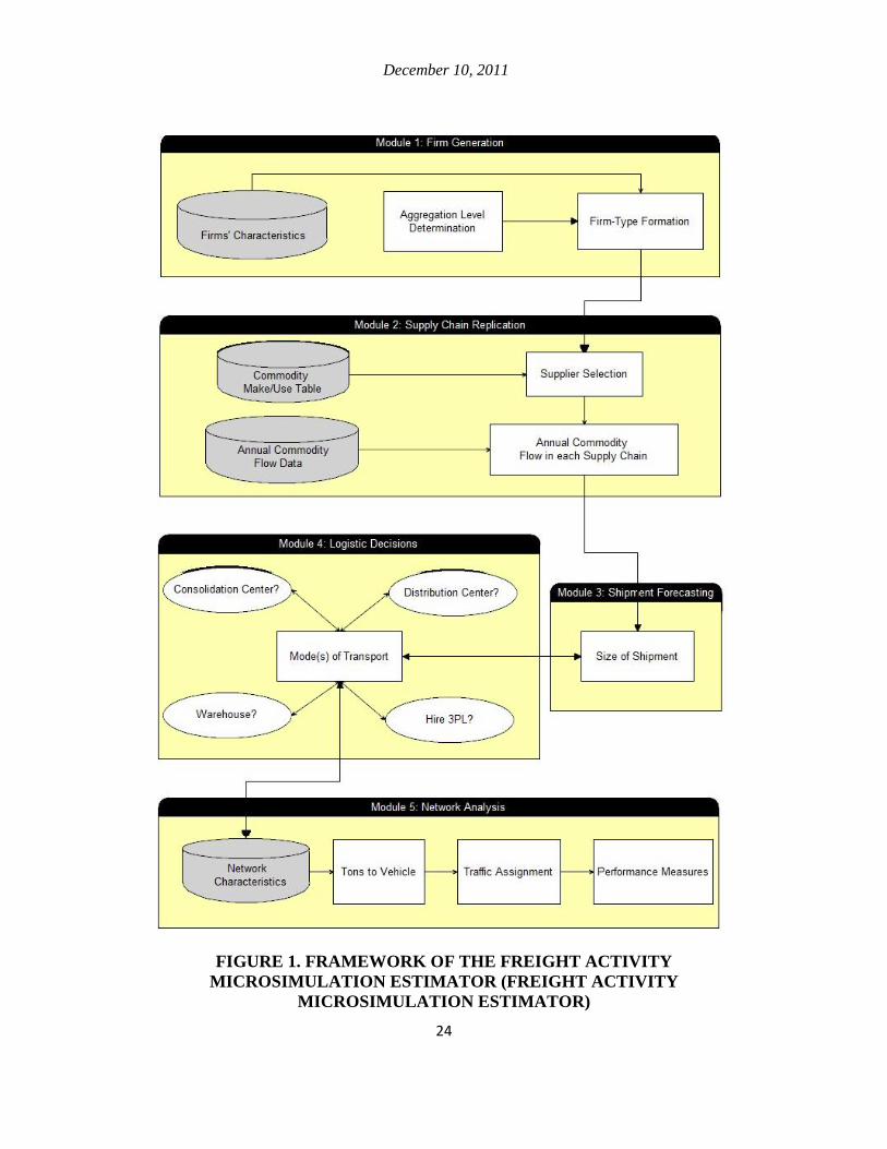
Freight Activity Microsimulation Estimator has five basic modules (Figure 1). In
the first module, Freight Activity Microsimulation Estimator recognizes all the firms in
the study area and identifies their basic characteristics. In the second module, Freight
Activity Microsimulation Estimator determines the types and amounts of incoming and
outgoing goods based on each firm’s characteristics and replicates their supply chain
designs. In the third module, Freight Activity Microsimulation Estimator defines
shipment sizes based on the previously collected data about the firms’ characteristics and
the way they trade commodities with each other. In the fourth module, Freight Activity
Microsimulation Estimator makes decisions regarding such areas as shipping mode, haul
time, shipping cost, warehousing, etc. Sophisticated firms simultaneously make
decisions on the supply chain’s physical infrastructure and logistics strategies. The study
team has treated these decisions separately in Freight Activity Microsimulation Estimator
to make the modeling structure compatible with the available data. In the last module,
Freight Activity Microsimulation Estimator investigates the goods movements’ impacts
on the transportation network.
In an ideal modeling structure, the above-mentioned modules are interrelated with
a recursive structure leading to more realistic results. For example, the results of the last
module, the network analysis, could help the model to better determine the shipping

December 10, 2011
23
mode. Similarly, the way logistic decisions are made in the fourth module could affect
the supply chain formation in the second module. Also, the general cost of commodity
transportation from the last module could be fed back into the second, third, and forth
modules, through numerous iterations, until a stabilized set of commodity flows and costs
are obtained. However, the chosen modeling framework is appropriate based on data
availability and the project’s scope of creating a forecasting tool that estimates national
movement and modal split. The effects of congestion are an important factor in route
selection at the urban area-level, but not at the national level.
December 10, 2011
24
FIGURE 1. FRAMEWORK OF THE FREIGHT ACTIVITY
MICROSIMULATION ESTIMATOR (FREIGHT ACTIVITY MICROSIMULATION ESTIMATOR)
December 10, 2011
25
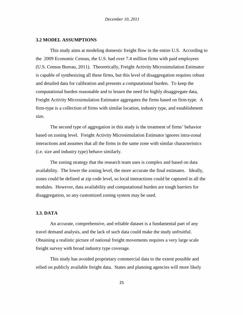
3.2 MODEL ASSUMPTIONS
This study aims at modeling domestic freight flow in the entire U.S. According to
the 2009 Economic Census, the U.S. had over 7.4 million firms with paid employees
(U.S. Census Bureau, 2011). Theoretically, Freight Activity Microsimulation Estimator
is capable of synthesizing all these firms, but this level of disaggregation requires robust
and detailed data for calibration and presents a computational burden. To keep the
computational burden reasonable and to lessen the need for highly disaggregate data,
Freight Activity Microsimulation Estimator aggregates the firms based on firm-type. A
firm-type is a collection of firms with similar location, industry type, and establishment
size.
The second type of aggregation in this study is the treatment of firms’ behavior
based on zoning level. Freight Activity Microsimulation Estimator ignores intra-zonal
interactions and assumes that all the firms in the same zone with similar characteristics
(i.e. size and industry type) behave similarly.
The zoning strategy that the research team uses is complex and based on data
availability. The lower the zoning level, the more accurate the final estimates. Ideally,
zones could be defined at zip code level, so local interactions could be captured in all the
modules. However, data availability and computational burden are tough barriers for
disaggregation, so any customized zoning system may be used.
3.3. DATA
An accurate, comprehensive, and reliable dataset is a fundamental part of any
travel demand analysis, and the lack of such data could make the study unfruitful.
Obtaining a realistic picture of national freight movements requires a very large scale
freight survey with broad industry type coverage.
This study has avoided proprietary commercial data to the extent possible and
relied on publicly available freight data. States and planning agencies will more likely

December 10, 2011
26
adopt models that can be developed using only widely available data. This section
elaborates data needs for Freight Activity Microsimulation Estimator and reviews some
data sets that the study team used in the model’s estimation.
The study team was required to gather the following: background on business
establishments, aggregate freight movement information, detailed information on a
sample of individual shipments and supply chains, and specifications on transportation
networks. Figure 2 summarizes where each data set is applied to the Freight Activity
Microsimulation Estimator framework.

December 10, 2011
27
Log
istic
s dec
isio
ns
Firm-type Generation
Introducing individual decision-makers with their characteristics and geographical distributions
Data Needed: Information on Business Establishment
Supplier selection
Determining trade relationships between firm-types
Data Needed: Information on Aggregate Freight Movement
Shipment size determining
Based on observed shipment size distribution
Data Needed: Information on individual shipments and supply chains
Mode choice
Using a probit model to select mode of transportation between Truck and Rail
Network analysis
Assigning commodity flows to the traffic network and assess the impacts
Data Needed: Specifications of the transportation network

December 10, 2011
28
FIGURE 2: FREIGHT ACTIVITY MICROSIMULATION ESTIMATOR
FRAMEWORK AND DATA NEEDS
3.3.1. Information on Business Establishments
An enormous number of American firms annually send or receive many
shipments. However, getting and processing this data is too difficult. The study team,
therefore, relied on firm-types for Freight Activity Microsimulation Estimator. They
used firm type, location, and number of employees to estimate the number of firms in
each type and assigned them to a particular geographic zone or zones. The publicly
available County Business Patterns dataset contains this data. The U.S. Census Bureau
has published the County Business Patterns dataset since 1964 (U.S. Census Bureau,
2008).
Annual information for all the U.S. business establishments with paid employees
during the week of March 12 is provided at the county level. This data is also available
for different geographic zones ranging from state to ZIP code levels. County Business
Patterns dataset provides the number of establishments, first quarter and annual payroll
by geographic area, industry, and employment size class. The County Business Patterns
dataset is the only complete and consistent source of county-level annual data for
business establishments with detail industry specification in the U.S. (U.S. Census
Bureau, 2009). A well-known problem with the County Business Patterns dataset's
disaggregate dataset is that a considerable number of values are not released due to
confidentiality issue. When the number of establishments drops below a predefined
value, the numbers are not reported. Although this is not a problem at the level of
aggregation used in this study, the missing values could be approximated using the
conventional methods, such as iterative proportional fitting if there is a need. Since most
of the aggregate numbers are provided for larger geographic areas and also for larger
industry classifications, the iterative proportional fitting is a promising approach to
address the issue of missing values (Auld et al., 2009).

December 10, 2011
29
With almost 1200 categories, the 2002 North American Industry Classification
System (NAICS) is used to classify industry type of businesses in the County Business
Patterns dataset (U.S. Census Bureau, 2010). The County Business Patterns dataset
provides a diverse range of industry classification resolution, from aggregate two-digit
North American Industry Classification System number to a fairly disaggregate six-digit
North American Industry Classification System number that is used in this study. Table 1
shows the two-digit industry codes and descriptions that is used in Freight Activity
Microsimulation Estimator. Table 2 presents summary statistics about U.S. business
establishments for the year 2002, obtained from the County Business Patterns dataset.
There were more than 7.2 million firms in the U.S. in the County Business Patterns
dataset 2002. The figure increased to around 7.7 million in 2007.
TABLE 1. TWO-DIGIT NORTH AMERICAN INDUSTRY CLASSIFICATION SYSTEM1
NAICS Code Description 11 Agriculture, Forestry, Fishing and Hunting 21 Mining 22 Utilities 23 Construction 31-33 Manufacturing 42 Wholesale Trade 44-45 Retail Trade 48-49 Transportation and Warehousing 51 Information 52 Finance and Insurance 53 Real Estate and Rental and Leasing 54 Professional, Scientific, and Technical Services 55 Management of Companies and Enterprises 56 Administrative and Support and Waste Management and Remediation Services 61 Educational Services 62 Health Care and Social Assistance 71 Arts, Entertainment, and Recreation 72 Accommodation and Food Services 81 Other Services (except Public Administration) 92 Public Administration 1 Source: http://www.census.gov/naics/

December 10, 2011
30
TABLE 2. U.S. BUSINESS ESTABLISHMENTS STATISTICS FOR THE YEAR 20021
NAICS Employees2 Annual payroll
($1000) Number of establishment by employment-size class
1-43 5-9 10-19 20-49 50-99 100-249 250-499 500-999 1000< Total 112400654 3943179606 3900755 1384960 912797 624628 210577 118724 30220 11377 6732 11 181162 4978291 17735 4641 2507 1219 289 126 26 7 2 21 465775 23961694 12389 3775 3386 2647 904 516 164 59 31 22 648254 41844745 7714 3060 2442 2553 1316 899 267 124 57 23 6307370 247302462 456597 119620 71197 43195 12444 5623 1182 339 128 31-33 14393609 580356005 123326 59889 53286 52301 25301 19748 6656 2638 1196 42 5860256 262527777 227405 85422 61877 41821 12406 6006 1391 435 137 44-45 14819904 320707026 517258 290121 170153 92079 31487 20326 3677 534 58 48-49 3581013 127251855 113061 29270 22721 18310 6757 3685 806 279 254 51 3536120 188076999 69551 21978 18365 15374 6669 4370 1347 652 284 52 6414583 372656276 258426 91878 53293 29660 8812 5189 1712 907 545 53 2017347 65241211 226343 53650 27786 10598 2826 1334 349 106 32 54 7046205 368778137 530713 113555 67898 39943 11672 6051 1649 597 287 55 2913798 204802311 19073 7128 6891 7031 3845 2967 1319 723 406 56 8299217 212189377 198062 50905 35732 28971 14442 10536 3120 1082 694 61 2701675 71961852 34326 11519 9901 10238 4078 2273 637 378 351 62 14900148 499177227 327337 166757 105986 60178 20687 15613 3519 1668 1795 71 1800991 47724377 65361 15093 11776 10869 4460 2073 462 164 117 72 10048875 131110795 202967 96210 106176 118831 32504 7096 903 290 172 81 5420087 118899903 455258 156968 78870 36479 8475 3339 558 125 46 95 1011496 52670905 3893 2236 2149 2265 1201 950 476 270 140 99 32769 960381 33960 1285 405 66 2 4 0 0 0 1 Source: http://www.census.gov/econ/cbp/ 2 Number of paid employees for the pay period that includes March 12. 3 Number of business establishment with less than five paid employees.
3.3.2. Aggregate Freight Movements
Two sets of information are explored in this section: annual commodity flows
between each zone pair, and relationship between different industries in the U.S.
economy.
3.3.2.1. Freight Analysis FrameworkAnnual value and tonnage of different commodity
types that are traded between the zone pairs are needed for the supply chain replication
in Freight Activity Microsimulation Estimator. The Federal Highway Administration

December 10, 2011
31
(2006) has utilized many freight data sources including but not limited to Commodity
Flow Survey (U.S. Census Bureau, 2007), Transborder Freight Transportation Data
(Bureau of Transportation Statistics, 2009), and Surface Transportation Board’s Rail
Waybill Sample to develop the Freight Analysis Framework. This dataset has the total
tonnage and value of shipments for each commodity type that are transported between all
the Freight Analysis Framework zone pairs for each mode of transportation. Some
federal publications, such as the annual Freight Facts and Figures (U.S. Department of
Transportation, 2009), provide descriptive statistics from the Freight Analysis
Framework. Even though the Freight Analysis Framework is the most comprehensive
publicly available freight dataset, it has a few limitations that make it insufficient for
some applications. One drawback is the level of geographical aggregation. The Freight
Analysis Framework divides the United States into 114 domestic regions and also
includes 17 international gateways, which is too large to use for local studies. Although
possible application of disaggregation methods to the Freight Analysis Framework
dataset has been examined to resolve this issue, no credible disaggregate Freight
Analysis Framework data has been made available at this time.
For a national level freight study; however, the Freight Analysis Framework
dataset provides valuable and creditable information. Therefore, the Freight Analysis
Framework estimates for the commodity flows between domestic zones is used as an
input. Two-digit Standard Classification of Transported Goods with 43 categories is used
in the Freight Analysis Framework to classify the commodities. The list of Standard
Classification of Transported Goods commodities is provided in Table 3. The same
commodity classification, i.e. 2-digit Standard Classification of Transported Goods, is
used in Freight Activity Microsimulation Estimator. Annual tonnage by commodity for
each domestic Freight Analysis Framework zone pair are imputed to the second module
of Freight Activity Microsimulation Estimator.

December 10, 2011
32
TABLE 3. STANDARD CLASSIFICATION OF TRANSPORTED GOODS
STANDARD CLASSIFICATION OF TRANSPORTED GOODS (SCTG)
2-DIGIT COMMODITY TYPES
SCTG Code Commodity Description
1 Live animals and live fish
2 Cereal grains
3 Other agricultural products
4 Animal feed and products of animal origin, n.e.c.1
5 Meat, fish, seafood, and their preparations
6 Milled grain products and preparations, bakery products
7 Other prepared foodstuffs and fats and oils
8 Alcoholic beverages
9 Tobacco products
10 Monumental or building stone
11 Natural sands
12 Gravel and crushed stone
13 Nonmetallic minerals n.e.c.1
14 Metallic ores and concentrates
15 Coal
16 Crude Petroleum
17 Gasoline and aviation turbine fuel
18 Fuel oils
19 Coal and petroleum products, n.e.c.1
20 Basic chemicals
21 Pharmaceutical products
22 Fertilizers
23 Chemical products and preparations, n.e.c.1
24 Plastics and rubber
25 Logs and other wood in the rough
26 Wood products
December 10, 2011
33
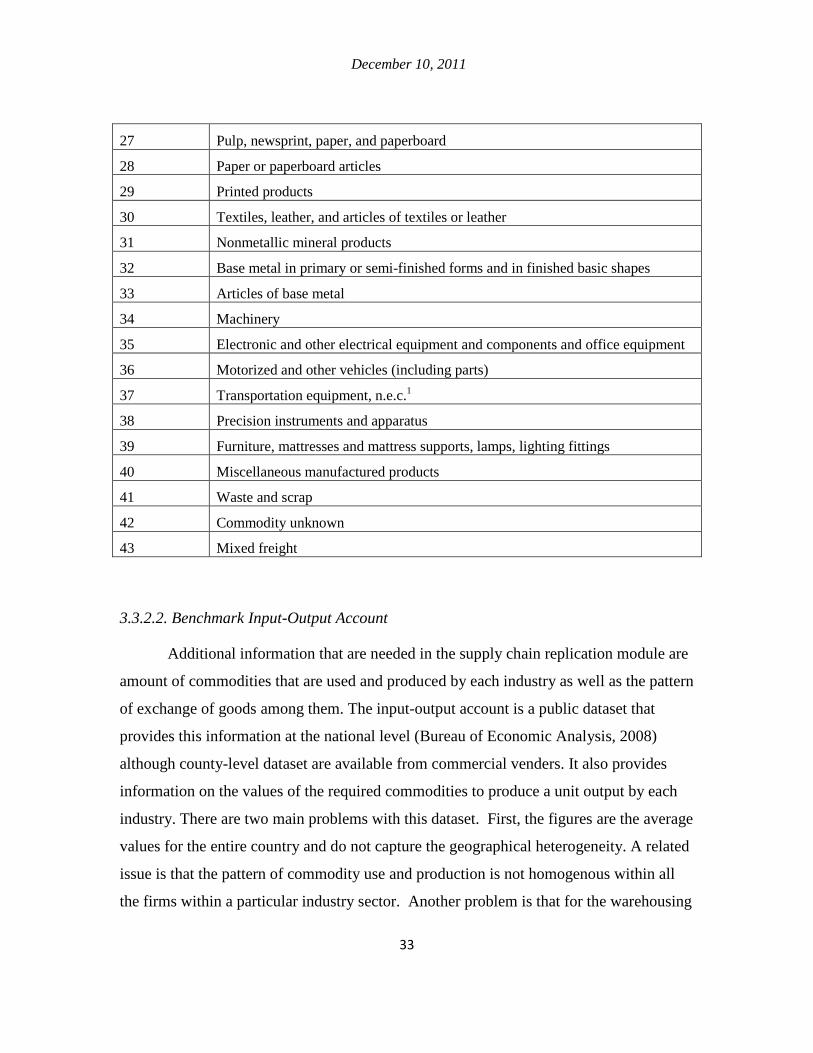
27 Pulp, newsprint, paper, and paperboard
28 Paper or paperboard articles
29 Printed products
30 Textiles, leather, and articles of textiles or leather
31 Nonmetallic mineral products
32 Base metal in primary or semi-finished forms and in finished basic shapes
33 Articles of base metal
34 Machinery
35 Electronic and other electrical equipment and components and office equipment
36 Motorized and other vehicles (including parts)
37 Transportation equipment, n.e.c.1
38 Precision instruments and apparatus
39 Furniture, mattresses and mattress supports, lamps, lighting fittings
40 Miscellaneous manufactured products
41 Waste and scrap
42 Commodity unknown
43 Mixed freight
3.3.2.2. Benchmark Input-Output Account
Additional information that are needed in the supply chain replication module are
amount of commodities that are used and produced by each industry as well as the pattern
of exchange of goods among them. The input-output account is a public dataset that
provides this information at the national level (Bureau of Economic Analysis, 2008)
although county-level dataset are available from commercial venders. It also provides
information on the values of the required commodities to produce a unit output by each
industry. There are two main problems with this dataset. First, the figures are the average
values for the entire country and do not capture the geographical heterogeneity. A related
issue is that the pattern of commodity use and production is not homogenous within all
the firms within a particular industry sector. Another problem is that for the warehousing

December 10, 2011
34
sector, the figures reported in the input-output table represent the amount of value-added
operations performed at facilities, instead of the value of the goods being stored or
transported through. There are county-level input-output data available from commercial
venders, but they are imputed from the national data and the accuracy of the county-level
data is unknown. Despite its drawbacks, considering the resources required to collect data
on economic activities throughout the country, national input-output account provides
rich information that can be used in the Freight Activity Microsimulation Estimator
model.
The 2002 benchmark input-output account covers more than 400 industries and
has its own industry classification system. The classification used for the input-output
account is similar to the six-digit North American industry classification system number,
but at a slightly higher aggregation level. To cope with this problem, the Bureau of
Economic Analysis has developed a crosswalk (i.e. an equivalency table) between the
six-digit North American industry classification system and this study’s input-output
account industry classification system.
The input-output account industry classification system provides information on
the transactions between the industries in monetary terms. Although this data is
extremely useful in the supply chain replication module, the input-output account does
not provide information on the linkages between commodity types and industry classes.
This information is critical since the Freight Analysis Framework data is provided for
commodity types instead of industry classes, and the Freight Activity Microsimulation
Estimator uses them to appropriate firm-types with specific industries. Fortunately, the
crosswalk that connects industry to commodity was developed during the Freight
Analysis Framework’s development; it has been incorporated into the Freight Activity
Microsimulation Estimator. This classification method for industry and commodity is
compatible with other data sources that are used in the Freight Activity Microsimulation
Estimator. It eliminates the error of making questionable assumptions and self-defined
crosswalks to link different data sources.

December 10, 2011
35
3.4. INFORMATION ON INDIVIDUAL SHIPMENTS AND SUPPLY CHAINS
After forming trade relationships between firm-types and determining annual
commodity flows between each pair of suppliers, the next step is to determine the
logistics choices (shipment characteristics, such as shipment size, mode, etc.) for these
flows. To develop logistics choice models in the third and forth modules, information on
individual shipments, such as shipping time, costs, mode, etc. are required. The detailed
specifications of the sending and receiving agents at different segments of the whole
shipping process should be collected to provide insights on the firms that are forming the
supply chain. For each acting agent in the whole shipping process, some information
including primary activity, employee size, annual turnover, establishment square footage,
number of franchises, etc. are of interest. Moreover, the shipment characteristics and
shipping specifications are needed. The former include the commodity’s weight, value,
dimensions, time sensitivity, type, origin, and destination, and the latter may be
comprised of the shipping process’ haul time, cost, mode, and damage risk.
Since there is no publically available data source of data for this data type,the
UIC team conducted an online business survey. This survey was specifically designed to
collect some information on shipments and facilitate development of the Freight Activity
Microsimulation Estimator. The study team carried out this survey in April and May of
2009. In total, 316 businesses participated in the survey and provided information on 881
shipments across the country. The survey detail and data quality analysis are included in
Appendix C.
3.5. SPECIFICATIONS OF THE TRANSPORTATION NETWORKS
Specifications of transportation networks are primarily needed for the fifth
module, network analysis. However, a rough estimate of the network characteristics for
each transportation mode is required in other modules as well. Accessibility to truck-rail
intermodal facilities, for example, is a critical element in a mode choice model and
should be obtained from transportation network data. The Oak Ridge National

December 10, 2011
36
Laboratory (2006) has developed a county-to-county distance matrix for the entire U.S.
Millage and impedance of all county pairs are estimated for rail, highway, water, and
highway-rail networks. Impedance values are mode specific and calculated for each link
based on several specifications. For example, impedance value for a link in the highway
network is affected by The presence of a divided roadway, level of access to the road,
rural or urban classification of the link, congestion level, etc. An intermodal link’s
impedance of is estimated in a way that accounts for the transfer time from truck to rail or
vice versa and that provides a more realistic general cost for using a transfer facility.
This data offers adequately accurate estimates for the characteristics of different
transportation networks, and has also been implemented in the 2002 Commodity Flow
Survey for estimating each mode’s ton-mile share.

December 10, 2011
37
CHAPTER 4. MODEL ESTIMATION
This chapter discusses the estimation of each module in the Freight Activity
Microsimulation Estimator model, except for the network analysis. A model’s estimation
involves finding the correct specification of mathematical equations and determining the
appropriate parameter values.
4.1. FIRM-TYPES GENERATION
As discussed earlier, the Freight Activity Microsimulation Estimator simulates
freight flows at the firm-to-firm level. Thus, the decision makers in this microsimulation
are individual firms in the U.S. There are more than 239,000 firms in the County
Business Patterns dataset. To keep the computational burden at a reasonable level and
diminish the need for highly disaggregate data, some form of aggregation is inevitable.
The Freight Activity Microsimulation Estimator uses firm types to aggregate firms with
similar characteristics into groups. A firm-type is a collection of firms with similar
location, industry type, and establishment size. It is assumed that firms with the same
characteristics have similar behavior in the freight decision-making process. Number of
firm-types can differ based on the number of industry types, establishment size, and
geographic zones in the study area.
4.2. SUPPLY CHAIN REPLICATION
In this step, supply chains are created by matching suppliers and buyers of goods.
All the potential suppliers for a given firm-type are determined in the first step and each
supplier’s suitability is assessed in the second step. Due to the modeling process’
technical nature, the study team only provides an overview of the approach they used for
this module . A detailed description of the modeling procedure involving the fuzzy
expert system’s development and application is included in Appendix A.
December 10, 2011
38
4.2.1. Generation of Candidate Suppliers
This procedure consists of two steps. In the first step, for a given type of
commodity, potential suppliers, expressed in terms of firm types, are determined. In
other words, the first stage of the supplier selection model is to list all the firm-types that
can sell a given product to a specific firm-type. Two conditions have to be met for a
firm-type to be eligible for such a list. First, the supplier should produce the commodity.
Second, the buyer has to need the supplier’s product as an input. The first step of the
supplier selection model estimates a probability for each of those two conditions for a
given supplier, buyer, and commodity type, and provides a degree of feasibility for a
certain supply chain to form by multiplying those figures. The method of estimating each
of the two probabilities is elaborated below.
The Freight Analysis Framework industry-to-commodity crosswalk was used to
estimate the probability that a supplier produces a given commodity, which is the first
condition. Almost all industry classes are linked to only one commodity type and thus
most of these probabilities are either zero or one.
The second step in determining supplier feasibility is to assess the probability that
the potential buyer’s industry class can use the supplier’s product. This figure is
estimated based on the supplier and buyer’s industry types, using the 2002 Benchmark
Input-Output Account. The standard use tables were applied at the six-digit North
American industry classification system level. This table contains the total value of a
given industry sector’s output that was used in different industry classes during 2002.
For example, the Glass Container Manufacturing sector sold 526.0 million dollars of its
products to the Fruit and Vegetable Canning, Pickling, and Drying sector; 13.5 million
dollars to the Cheese Manufacturing sector ; 2,042.4 million dollars to the Breweries
sector; 552.2 million dollars to the Wineries sector; and so on. These figures were used
to calculate the percentage of a given industry’s output that other industry sectors used.

December 10, 2011
39
4.2.2. Evaluation of Candidate Suppliers
The second stage in the supplier selection model is to assess the candidate
suppliers’ suitability. As argued earlier, there is no comprehensive dataset with specific
information about supplier selection behaviors in different industry sectors across the
country. Therefore, the study team used a fuzzy rule-based expert system, which is not
data intensive to evaluate each potential supplier’s suitability.
Some recent supply chain management studies have highlighted the benefits of
fuzzy rule-based systems compared to mathematical optimization approaches. Altinoz
(2008) argued that incomplete information about the candidate suppliers and the
methodology’s complexity seriously limit the usability of mathematical optimization
approaches. He evaluated the usability level of different supplier selection
methodologies by practitioners and proposed a fuzzy rule-based expert system.
According to Zadeh (1965), the fuzzy logic system could effectively model a complex
system, while avoiding explicit mathematical formulations. The major components of
the fuzzy rule-based systems, introduced here are discussed in Appendix A.
4.3. SHIPMENT SIZE DETERMINATION
A shipment size model provides a categorical output variable with three clusters:
small (less than 1,000 lb), medium (1,000-50,000 lb), and large (more than 50,000 lb).
This model is required for the Freight Activity Microsimulation Estimator’s third module,
where the sizes of individual shipments are determined. In other words, annual flow of a
specific commodity between a given supplier and buyer pair has to be broken down into
single shipments. Such model’s output could be each shipment’s weight in pounds or just
a categorical variable in the form of weight range. The former, being a continuous
variable, provides richer information for each shipment, but requires more precise data
and method for estimation. The latter is less data intensive but has a higher uncertainty
level. Given this study’s nationwide scope and data limitation, the study team could not
carry out the logistic cost minimization approach. Instead, the study team obtained the

December 10, 2011
40
distribution of the shipment size for each commodity type and shipping distance category
from the 2002 Commodity Flow Survey. This information was used with other
procedures to determine the sizes of individual shipments in a categorical output variable
in three weight ranges: small, medium, and large.
Shipment size distribution in this study is initially set in a way that larger
suppliers and buyers tend to ship their annual commodity flow in larger shipments. After
initialization, a modified iterative proportional fitting approach was applied to replicate
the shipment size distribution that was observed in the 2002 Commodity Flow Survey to
the extent possible. The Commodity Flow Survey data has reported nationwide annual
tonnage of transported commodities in a three dimensional table: commodity type,
shipping distance, and shipment size. Similar to this study, commodities are classified in
two digits Standard Classification of Transported Goods. Shipping distance is provided in
nine categories (<50 miles, 50-99, 100-249, 250-499, 500-749, 750-999, 1000-1499,
1500-2000, >2000), and shipment size is also given in nine categories (<50 lbs., 50-99,
100-499, 500-749, 750-999, 1000-9999, 10000-49999, 50000-99999, 100,000<). The
supplier and buyer’s establishment size, shipping distance, and commodity type are
inputs to this process. The model was applied on the annual commodity flow between
each supplier and buyer pair from the supply chain replication module to determine the
shares of small, medium, and large shipments accordingly. However, knowing that a
shipment is small is not sufficient for the modal split in the next module. Mode split
requires a crisp value for the shipment size. Conversion of the shipment size class to
specific value was carried out using the distribution of observed shipment sizes from the
UIC National Freight Survey. Details of the shipment size model and shipment size
distributions are elaborated in Appendix B.
4.4. MODE CHOICE MODEL
Mode choice is the most critical logistics decision. A proper choice model should
be sensitive to the decision-maker’s attributes and to the choice alternatives. Unlike the

December 10, 2011
41
decision-maker’s characteristics, the attributes of choice alternatives vary significantly
from one alternative to the other. As previously mentioned, to obtain the necessary
information for developing the modal split model of the Freight Activity Microsimulation
Estimator, the study team carried out a nationwide survey of businesses. The survey data
satisfied the data needs for developing a mode choice model and also other components
of the Freight Activity Microsimulation Estimator framework. The detail of the survey
and the survey results analysis are included in Appendix C.
The survey is the only data source for the Freight Activity Microsimulation
Estimator that is not publically available. To achieve the goal of developing a model that
can only be used only with publicly available data, this document includes the two freight
mode choice model specifications that were calibrated based on the UIC National Freight
Survey. Depending on the availability of input variables, agencies will be able to select
the powerful yet data hungry model or the parsimonious model that requires a limited
number of input variables.
First, the consultant team developed an explanatory model to shed light on truck
and rail (including truck-rail intermodal) competition in the U.S. freight transportation
market. Some of the explanatory variables in the model were not available, however,
from publically available sources. The study team proposed a parsimonious mode choice
model that is better suited for practical use the microsimulation. Although the latter had a
modest set of input variables, its overall goodness of fit was slightly less than the
explanatory model.
The Limdep econometrics software (Greene, 2002) was used in this study for the
mode choice model calibration. Akaike and McFadden values along with the chi-squared
values were used for model selection (Train, 2003). The higher the McFadden value and
the lower the Akaike measure, the better the explanatory power of the model. Standard t-
statistics were used to test whether each coefficient had a non-zero effect on the choice
probability. Wald, Likelihood Ratio, and Lagrange Multiplier tests, known as Neyman-

December 10, 2011
42
Pearson tests (Greene, 2002), were also carried out to assess the overall significance of
the final models.
Percentage of correctly predicted observations, which is often used to validate
mode choice models, is usually high in binary choice models that include a rare event as
one of the choices. In many cases, the high accuracy figure could be misinterpreted as
the indicative of the general explanatory power of the model. When one of the two
possible choices is very rare and the other is common, binary models tend to over-predict
the latter, resulting in a high rate of correct predictions at the expense of largely ignoring
the rare event outcomes. For example, if 99 out of 100 data points in the dataset chose
the common alternative, the model can attain 99% accuracy by simply predicting all
cases to be common, but the model lacks the sensitivity to its input variables and
consequently provides very little information. In Freight Activity Microsimulation
Estimator, choosing the rail mode over truck could be considered as a rare event with less
than 10% chance of occurrence in the data. Both mode choice models developed for
Freight Activity Microsimulation Estimator achieved satisfactory accuracy in predicting
rail shipments.
Potential multicollinearity between explanatory variables is also controlled in two
ways. Large off-diagonal values were searched in the variance-covariance matrices as
the primary effect of multicollinearity. Meanwhile, variance inflation factors (VIFs) were
estimated for all the independent variables to detect any severe multicollinearity among
the explanatory variables. Kutner et al. (2004) suggested a variance inflation factor of 5
as the threshold that indicates a presence of serious multicollinearity. Following sections
provides a detailed discussion of the development of the mode choice models.
4.4.1. Explanatory Model
Variables that were used in the development of the mode choice models are
shown in Table 4. Table 5 shows the specifications of the exploratory model along with
the assessment of it performance. All the estimated parameters in the exploratory models

December 10, 2011
43
turned out to be significant with a p-value of less than 0.05, and most of them are
significant with a 99% confidence interval. The model has a pseudo R-squared value of
over 57%, and are able to correctly predict 95% of the observations. As noted before, the
model predicted more than 72% of rail shipments correctly. As shown in Table 5, none of
the variables had a variance inflation factor in excess of 3.5, and thus, multicollinearity is
not an issue in this model.
4.4.2.Parsimonious Model
Although the exploratory model revealed some behavioral aspects of modal
selection such as different levels of sensitivity to travel time and cost for truck and rail
users, it is not necessarily a good model to be implemented in a microsimulation or
forecasting. For example, the explanatory mode choice model could not be used in a
nationwide microsimulation effectively since time and cost of each mode should be
estimated for all the simulated shipments prior to determining the mode, which is an
extremely challenging if not impossible task. Therefore, another model with a
parsimonious nature is discussed here. The model achieved a slightly less goodness of fit,
but only uses a set of explanatory variables that are much easier to obtain. Basic
descriptive statistics of variables that are used in this model are summarized in Table 6.
TABLE 4. VARIABLES USED IN THE EXPLANATORY MODEL
Variable Definition Mean Standard deviation
MODE 1: rail or any combination of that with other modes / 0: truck 0.089 0.285
DISTANCE Suggested distance between origin and destination by Google Map (miles) 1077 2221
WEIGHT Weight of the shipment (lbs) 22901 25275 VALUE Value of the shipment (USD) 48101 130150 TRUCK-COST Shipping cost by truck (USD) 1331 4093 RAIL-COST Shipping cost by rail (USD) 2016 1128 TRUCK-TIME Shipping time by truck (days) 2.012 1.357 RAIL-TIME Shipping time by rail (days) 7.281 6.662 TRUCK-COST-INDEX = Ln (TRUCK-COST / (TRUCK-TIME * VALUE)) -3.542 1.521 RAIL-COST-INDEX = Ln (RAIL-COST / (RAIL-TIME * VALUE)) -3.705 1.940 SAME-DECISION 1: if the same mode was preferred TWO years ago 0.934 0.248

December 10, 2011
44
for a similar shipment / 0: otherwise
ACCESS 0: firm has easy access to truck rail intermodal facilities / 1: neutral access / 2: difficult access 0.780 0.415
POTENTIAL-INTERMODAL 1: truck-rail intermodal is considered always or often as a potential transportation mode / 0: otherwise 0.349 0.477
PERISHABLE 1: if the commodity is perishable / 0: otherwise 0.160 0.367
CONSOLIDATION-CENTER 1: if the shipment has gone through a consolidation center / 0: otherwise 0.143 0.350
DISTRIBUTION-CENTER 1: if the shipment has gone through a distribution center / 0: otherwise 0.270 0.445
WAREHOUSE 1: if the shipment has gone through a warehouse / 0: otherwise 0.347 0.477
DECISION-MAKER 1: if a 3PL company has make the shipping decision / 0: otherwise 0.104 0.305

December 10, 2011
45
TABLE 5. EXPLANATORY MODE CHOICE PROBIT MODEL
Item Value t-ratio VIF C
oeff
icie
nt
CONSTANT -5.902 * -6.050 - DISTANCE 0.237E-03 ** 2.273 2.776 WEIGHT 0.310E-04 * 4.293 1.564 TRUCK-TIME 0.622 * 5.019 1.648 RAIL-TIME -0.094 * -2.579 2.387 TRUCK-COST-INDEX 0.388 ** 2.532 3.408 RAIL-COST-INDEX -0.659 * -3.474 1.099 POTENTIAL-INTERMODAL 1.214 * 3.468 2.776
Fit M
easu
res
Log likelihood -47.1 - - Model Chi-squared 128 - - Akaike I.C. 0.296 - - Pseudo R-squared 0.577 - - Correctly Predicted (%) 95.4 - - Correctly Predicted (%) –rail 72.7 - -
TABLE 6. VARIABLES USED IN THE PARSIMONIOUS MODEL
Variable Definition Mean Standard deviation
MODE 1: truck / 0: rail or any combination of that with truck 0.924 0.263 GCD Great circle distance (miles) 616 640 WEIGHT Weight of the shipment (lbs) 23457 28959 IMPEDANCE* = EXP (H_IMP/R_IMP) 6.186 3.338 H_IMP Highway impedance 897 4589 R_IMP Rail impedance 1176 9082 CONTAINERIZED 1: if the shipment is containerized / 0: otherwise 0.0229 0.149
COMMODITY 1: if the commodity is agricultural, chemical, pharmaceutical, gravel, natural sands, cement, machinery, metal, mixed freight, or prepared foodstuffs / 0: otherwise.
0.655 0.475
* The Oak Ridge National Laboratory (27) has provided county-to-county distance matrix for the entire U.S. and impedance for every county pairs are estimated in rail, highway, water, and highway-rail networks. Impedance units are mode specific and Impedance values are mode specific and calculated for each link based on several specifications such as length and type of a road to bring the approximate costs into common units. For example, impossible routes (eg,

December 10, 2011
46
highway from California to Hawaii) have a mileage of -1.0 and an impedance of 99999.9 in this dataset. The study team prefers a probit specification for this model What is a probit
specification? Although logit models assume the error terms in the utility function to be
independently and identically distributed ( commonly referred to as an “IID.
assumption”), it has a closed-form equation for estimating the probability of each choice.
This makes logit models convenient to use, especially in microsimulations that requires
numerous iterations. Probit models do not require the IID assumption, but do require a
numerical method for estimating the probability of each choice. For binary probit models
such as the Freight Activity Microsimulation Estimator mode choice models, however,
the task does not pose an insurmountable challenge.
Table 7 shows the parsimonious probit model that estimates the probability of
choosing between truck and rail / truck-rail modes. All of the estimated parameters in the
model are significant with a p-value of less than 0.05. The model has a pseudo R-squared
value of 54%, and correctly predicts 96% of the observations. Furthermore, more than
58% of rail or truck-rail shipments are correctly predicted. As shown in Table 7, all the
variance inflation factors are less than five. Thus, a serious multicollinearity is not
detected.
TABLE 7. PARSIMONIOUS MODE CHOICE PROBIT MODEL
Item Value t-ratio VIF
Coe
ffic
ient
CONSTANT 4.83 8.170 - GCD * -.104E-02 -4.856 2.078 WEIGHT* -.254E-04 -5.075 1.029 IMPEDANCE ** -.988E-01 -1.978 2.021 CONTAINERIZED* -1.27 -2.612 1.055 COMMODITY* -.940 -2.985 1.046
Fit M
easu
res
Log likelihood -58.5 - - Model Chi-squared 138.4 - - Akaike I.C. 0.269 - - Pseudo R-squared 0.541 - - Correctly Predicted (%) 95.61 - - Correctly Predicted (%) –rail 58.33 - -

December 10, 2011
47

December 10, 2011
48
CHAPTER 5. MODEL IMPLEMENTATION AND VALIDATION
This chapter discusses the procedures used to apply a complete set of data to the
Freight Activity Microsimulation Estimator. The outputs from each module of the
Freight Activity Microsimulation Estimator are compared against real-world data to
assess the models’ validity.
5.1. FIRM-TYPES GENERATION
A total of 45,206 firm-types were generated for the microsimulation of the
domestic Freight Analysis Framework zones. The study team considered 123 domestic
Freight Analysis Framework zones, 328 industry classes (North American Industry
Classification System), and eight employee size groups (Table 8) in this simulation. All
the industry classes in the Freight Analysis Framework, at the 2-digit Standard
Classification of Transported Goods, are considered in Freight Activity Microsimulation
Estimator, but the industry classes for which no business establishment was reported in
2007 County Business Patterns dataset are excluded except for North American Industry
Classification System 111150 (corn farms) which is considered in the simulation process
by using a calibration method in the Freight Activity Microsimulation Estimator input
data.
TABLE 8. DEFINITION FOR ESTABLISHMENT SIZE CLASSIFICATION
Establishment size category Range of number of employees
1 1 – 19 2 20 – 99 3 100 – 249 4 250 – 499 5 500 – 999 6 1000 – 2499 7 2500 – 4999

December 10, 2011
49
8 4999 <
5.2. SUPPLY CHAINS REPLICATION
Supply chains were replicated using the approach that was explained in the
previous chapter. As a quick reminding note, this model scores the appropriateness of all
the possible suppliers for a given firm-type. Using the likelihood of partnership for any
pair of supplier and buyer, annual commodity flows can be disaggregated from the
Freight Analysis Framework zone level into the firm-type level. For a given origin,
destination, and commodity type combination, value of total annual tonnage was
disaggregated among the top 5% of supplier and buyer pairs with the highest
appropriateness score. This score was weighted by the total number of actual firms within
the supplying and buying firm-type before disaggregation. This was to distinguish
between a pair of supplier and buyer with only one actual firm in each side of the chain
from those with several actual firms in each side. Obviously, the latter should receive a
higher share of commodity fellow.
As mentioned previously, all the Freight Analysis Framework industry sectors
were considered in Freight Activity Microsimulation Estimator, but some of them were
not present in some of the zones in the simulation. This is due to the limitations in the
business establishment data sources and also the crosswalks that were used in the second
module. As a result, not all of the Freight Analysis Framework commodity flows between
the zone pairs was allocated to firm-types. In some rare cases, a specific type of
commodity is entirely ignored. For instance, alcoholic beverages were not simulated from
zone number 79 to 48. This is because there was no provider for that specific commodity
in the origin nor a buyer in the destination zone according to the County Business
Patterns dataset. Furthermore, there is no flow of live animals and live fish, unknown
commodities, and mixed freight in the microsimulation, although those are reported in the
Freight Analysis Framework. This is because industry that is associated with the
aforementioned commodity types are not covered by the County Business Patterns
dataset. In the Freight Analysis Framework, a total of 13,140,649,051 tons of commodity

December 10, 2011
50
valued at around 8,794,018 billion dollars is transported between the domestic origin and
destinations on truck, rail, or truck-rail intermodal. In contrast, 10,583,089,838 tons of
commodity valued at around 6,944,709 billion dollars is simulated in Freight Activity
Microsimulation Estimator. Thus, around 80% of the Freight Analysis Framework
domestic tonnage and 79% of commodity values are simulated in this study.
5.3. SHIPMENT SIZE DETERMINATION
The proposed shipment size model estimates a categorical output variable with
three clusters: small, medium, and large. This model was applied to the annual
commodity flow between each pair of supplier and buyer to determine the shares of
small, medium, and large shipments accordingly. Then, the data from the survey were
used to estimate the actual value of the shipments. We found that Beta distribution
produced a good fit with the surveyed data. Beta distribution has the added benefit of
having lower and upper bounds on the distribution. A Q-Q plot for each shipment size
class, depicted in Figures 3, 4, and 5, show the fit of the model for small, medium, and
large shipment size, respectively. In Q-Q plots, observed values are plotted against fitted
values. Q-Q plots could be used as a nonparametric approach to compare shapes of two
distributions, providing a graphical assessment of goodness of fit. In our case, if the
specified distribution is a decent model, the Q-Q plot will be approximately lying on the
line 45-degree line. This reference diagonal line is also drawn in the figures to indicate
where the graph points should ideally fall. The shape parameters of each beta distribution
that are used in this simulation are provided in Table 9.
TABLE 9. SHAPE PARAMETERS OF THE BETA DISTRIBUTIONS FOR SHIPMENT SIZE
Shipment Size Alpha Beta Upper Limit Lower Limit
Small 0.436 0.914 1 1000
Medium 0.530 0.593 1001 50000
Large 0.090 0.243 50001 200000

December 10, 2011
51
FIGURE 6. Q-Q PLOT, COMPARING OBSERVED AND PROPOSED DISTRIBUTION FOR SMALL SHIPMENTS

December 10, 2011
52
FIGURE 7. Q-Q PLOT, COMPARING OBSERVED AND PROPOSED
DISTRIBUTION FOR MEDIUM SHIPMENTS

December 10, 2011
53
FIGURE 8. Q-Q PLOT, COMPARING OBSERVED AND PROPOSED DISTRIBUTION FOR LARGE SHIPMENTS.
5.4. MODE SPLIT
The research team used a binary mode choice model in this simulation to
determine the share of truck and rail (including truck-rail intermodal) used for each
shipment. The research team had to determine all of the following variables for each
simulated shipment: shipment distance measured in great circle distance, weight, relative
impedance between truck and rail, a dummy for containerized shipments, and commodity
type.
Since the origin and destination zones are known, the research team could obtain
the great circle distance and relative impedance from the intercounty distance matrix,
which the Oak Ridge National Laboratory provided in 2006.
The research team also estimated each shipment’s weight in the shipment size module.
The research team also knew the two-digit Standard Classification of Transported Goods
commodity type for each simulated shipment and therefore could accordingly determine
the dummy variable for each commodity type’s containerized shipments. These variables
were drawn from Bernoulli distributions. Bernoulli is a discrete probability distribution
with a given success probability.
In this simulation, the research team assumed that the overall probability of
having containerized shipments was 11.8%, based on the UIC National Freight Survey.
The research team, however, weighted this figure by the normalized highway impedance
between each origin and destination that the Oak Ridge National Laboratory (2006)
provided to account for the relationship between shipment distance and the probability of
containerization. Since the weight factors were normalized, the average chance of having
a containerized shipment remained the same. However, this chance was higher for long
haul shipments. Although the binary mode choice overall has a satisfactory goodness of
fit, it tends to underestimate the total number of rail shipments. Therefore, the research

December 10, 2011
54
team multiplied the estimated probability of a rail shipment by 1.3 to adjust for this
underestimation.
Given the microsimulation’s random nature, the research team repeated the
simulation 20 times. Table 10 shows each run’s results, mean, and variation coefficient.
Although the model provided each mode’s shipment tonnage, the research team
estimated each shipment’s dollar value. They multiplied the average dollar per ton to the
shipment tonnage for each commodity type in the Freight Analysis Framework’s
Standard Classification of Transported Goods. They also estimated the shipment ton-
miles using the intercounty distance matrix, which the Oak Ridge National Laboratory
provided in 2006.

December 10, 2011
55
TABLE 10 RELATIVE PERCENTAGE OF TRUCK-ONLY SHIPMENTS IN
DIFFERENT SIMULATION RUNS
Simulation Run Ton Value Ton-mile 1 79.63% 89.92% 65.62% 2 79.87% 90.19% 66.37% 3 79.26% 90.14% 67.43% 4 79.65% 89.79% 68.18% 5 78.34% 89.72% 60.99% 6 78.39% 89.82% 65.21% 7 78.04% 89.82% 60.75% 8 78.98% 89.85% 65.20% 9 78.85% 89.85% 62.86% 10 78.73% 89.92% 66.16% 11 79.77% 89.89% 64.60% 12 80.21% 90.26% 62.48% 13 80.14% 89.87% 65.22% 14 79.10% 89.97% 63.35% 15 77.39% 89.78% 63.61% 16 79.70% 89.93% 64.15% 17 78.43% 89.51% 64.22% 18 79.04% 90.03% 67.43% 19 80.49% 90.23% 68.11% 20 79.57% 90.30% 62.82% Mean 79.18% 89.94% 64.74% Coefficient of Variation 0.98% 0.22% 3.28%
5.5. VALIDATION
This study’s primary objective was to develop a behavioral freight model that
focuses on truck and rail modes. The mode share for the two modes is therefore
expressed in total tonnage, value, and ton-mile of commodities (Table 11) and is
validated in this section. The research team compared the Freight Activity
Microsimulation Estimator’s estimated values against those from the Freight Analysis
Framework and the Commodity Flow Survey, two major public freight data sources in
the U.S. It should be noted that modal split information from these datasets have not
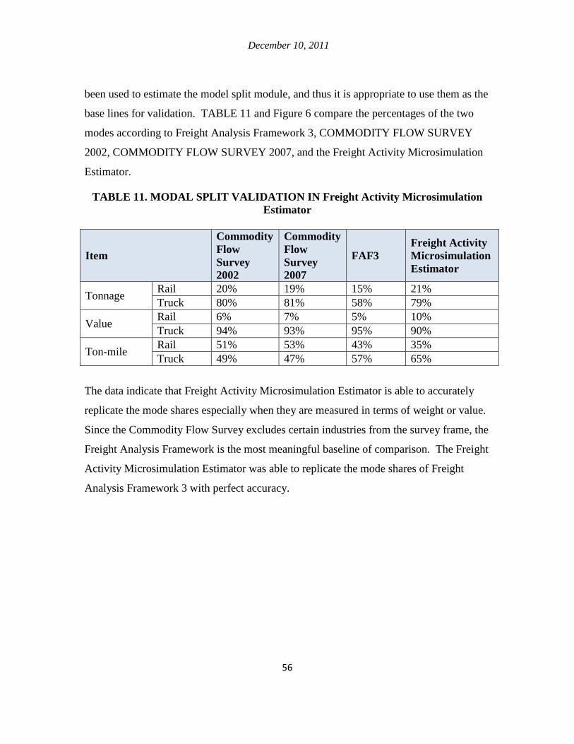
December 10, 2011
56
been used to estimate the model split module, and thus it is appropriate to use them as the
base lines for validation. TABLE 11 and Figure 6 compare the percentages of the two
modes according to Freight Analysis Framework 3, COMMODITY FLOW SURVEY
2002, COMMODITY FLOW SURVEY 2007, and the Freight Activity Microsimulation
Estimator.
TABLE 11. MODAL SPLIT VALIDATION IN Freight Activity Microsimulation Estimator
Item
Commodity Flow Survey 2002
Commodity Flow Survey 2007
FAF3 Freight Activity Microsimulation Estimator
Tonnage Rail 20% 19% 15% 21% Truck 80% 81% 58% 79%
Value Rail 6% 7% 5% 10% Truck 94% 93% 95% 90%
Ton-mile Rail 51% 53% 43% 35% Truck 49% 47% 57% 65%
The data indicate that Freight Activity Microsimulation Estimator is able to accurately
replicate the mode shares especially when they are measured in terms of weight or value.
Since the Commodity Flow Survey excludes certain industries from the survey frame, the
Freight Analysis Framework is the most meaningful baseline of comparison. The Freight
Activity Microsimulation Estimator was able to replicate the mode shares of Freight
Analysis Framework 3 with perfect accuracy.

December 10, 2011
57
CHAPTER 6. CONCLUSION
The primary motivation for this research was to develop a behavioral freight
mode choice model for Northeastern Illinois. Since the freight flow in Northeastern
Illinois is intimately connected to the national movement of goods, the research team
developed a nationwide freight activity microsimulation model. This is a monumental
achievement as in the past. Although the need to incorporate freight movement in the
broader national transportation policy framework is recognized, development of
satisfactory analysis tools to facilitate decision-making is highly challenging given the
complexity of the decision-making process, a lack of an acceptable freight modeling
framework, and scarcity of freight data.
This report’s modeling framework replicates shipping behaviors to incorporate
firms’ characteristics and seeks to pave the way for future behavioral freight
microsimulation efforts. This research has already made significant impacts in freight
demand analysis in the Chicago region as two ambitious efforts, one by the Chicago
Metropolitan Agency for Planning (CMAP), and the other by the Federal Highway
Administration (FHWA), rely heavily on this study’s approach, and its output, in some
cases.
A major drawback of many previous efforts of this kind was their aggregate
nature which prevented the development of an actor-based microsimulation. This
limitation has seriously affected the models’ reliability and applicability in the
environment where firms are increasingly relying on supply chain management concepts
to remain competitive. The conventional models are not able to reconcile the
proliferation of e-commerce, information technologies, and sophisticated supply chain
management strategies with freight shipment decision-making processes.
The Freight Activity Microsimulation Estimator is one of the first attempts to
address these problems by incorporating behavioral factors in a microsimulation
framework. Its geographical coverage also is broader than most of the past models, thus

December 10, 2011
58
giving policymakers and agencies a powerful tool for analyzing and evaluating potential
courses of action to meet the many challenges facing the movement of goods in the U.S.
and Northeastern Illinois in particular.
The research team strived to develop a sound microsimulation freight model in
this study as a valid forecasting tool that could contribute to more reliable policy
assessments compared to existing decision-making tools. The proposed framework (the
Freight Activity Microsimulation Estimator) has some remarkable characteristics that
distinguish it from other frameworks:
• The Freight Activity Microsimulation Estimator is mostly based on
publicly available freight data. Combined with the on-line survey that was
developed to collect key pieces of data that were not publicly available,
the Freight Activity Microsimulation Estimator’s data collection cost is
modest compared to that of other behavioral models.
• It is one of the early efforts in freight demand modeling that has a separate
component for simulating the formation of supply chain configurations. A
fuzzy expert system was developed for supplier selection. This approach
could be used in the absence of disaggregate data on supply chain
formation.
• The Freight Activity Microsimulation Estimator has an open structure and
could accept other components that may become available later.
• The Freight Activity Microsimulation Estimator covers almost all the
industry classes in the U.S.
• The Freight Activity Microsimulation Estimator has a unique geographic
coverage and is probably the first comprehensive nationwide freight
microsimulation in the U.S.
This study designed and implemented a cost-effective way of collecting
disaggregate freight data for running this simulation. An online establishment survey that

December 10, 2011
59
was conducted as part of this research provided valuable disaggregate information that
was necessary for developing a behavioral freight model. The research team looked for
the presence of a selection bias that is common in surveys with low response rates, but
found no serious issues.
The research team also calibrated two freight mode choice models based on the
UIC National Freight Survey. They first developed an explanatory model to gain insights
on truck and rail (including truck-rail intermodal) competition in the U.S. freight
transportation market. They later developed a parsimonious mode choice model for use
in the microsimulation. They built this model using only variables that are easy-to-obtain
or estimate from existing data. Its overall goodness of fit was only slightly less than the
explanatory model. We believe that this model is superior to the existing mode choice
models used in practice, and should attract interest from agencies around the country.

December 10, 2011
60
CITED LITERATURE
AASHTO, Invest in America- Freight Rail Bottom Line Report. January 2003.
Abdelwahab, W. M. (1998) Elasticities of Mode Choice Probabilities and Market Elasticities of Demand: Evidence from a Simultaneous Mode Choice/Shipment-Size Freight Transport Model. Transportation Research Part E: Logistics and Transportation Review 34(4): 257-266.
Abdelwahab, W., and M. Sargious (1992) Modelling the Demand for Freight Transport: A New Approach. Journal of Transport Economics and Policy, 26(1): 49-70.
Ahanotu, D., and A. Mani (2008) Freight Data Synthesis. Final Report No. CDOT-2008-3, Colorado Department of Transportation Research Branch.
Al-Deek, H. Comparison of Two Approaches for Modeling Freight Movement at Seaports. The ASCE Journal of Computing in Civil Engineering, 15(4), pp. 284-291, 2001.
Allen, J. and M. Browne (2008) Review of Survey Techniques Used in Urban Freight Studies. Project Report of the Green Logistics: Work Module 9 (Urban Freight Transport).
Arunotayanun, K., and J. W. Polak (2007) Taste Heterogeneity in Freight Shippers’ Mode Choice Behaviour. Proceedings, 86th Annual Meeting of the Transportation Research Board, Washington DC, 21–25 January 2007.
Altinoz, C., (2008) Supplier selection for industry: a fuzzy rule-based scoring approach with a focus on usability. International Journal of Integrated Supply Management, Vol. 4, pp. 303 - 321.
Auld, J., Mohammadian A. and Kermit, W. (2009). “Population Synthesis with Subregion-Level Control Variable Aggregation.” Journal of Transportation Engineering, 135(9), 632-639.
Baumol, W. J., and H. D. Vinod (1970) An Inventory Theoretic Model of Freight Transport Demand. Management Science, 16(7): 413–421.
Bezdek, J. C. (1981) Pattern Recognition with Fuzzy Objective Function Algorithms. Plenum Press, New York.

December 10, 2011
61
Boerkamps, J. H. K., A. J. van Binsbergen, and P. H. L. Bovy (2000) Modeling Behavioral Aspects of Urban Freight Movement in Supply Chains. Transportation Research Record, 1725: 17-25.
Brogan, J. J., S. C. Brich, and M. J. Demetsky (2001) Application of a Statewide Intermodal Freight Planning Methodology. Final Report VTRC 02-R5.
Bryan, J., G. Weisbrod, C. D. Martland (2007) Rail Freight as a Means of Reducing Roadway Congestion: Feasibility Considerations for Transportation Planning. Transportation Research Record, 2008: 75-83.
Bureau of Economic Analysis. 2008. Revised 2002 Benchmark Input-Output Make and Use Tables. http://www.bea.gov/industry/Make_Use_table_revisions.htm, Accessed December 24, 2008.
Bureau of Transportation Statistics. 2004. 2002 Commodity Flow Survey (COMMODITY FLOW SURVEY) United States. http://www.bts.gov/publications/commodity_flow_survey/2002/united_states, Accessed May 2, 2008.
Bureau of Transportation Statistics. 2007 Commodity Flow Survey (COMMODITY FLOW SURVEY) Preliminary Tables. United States, 2008. http://www.bts.gov/publications/commodity_flow_survey/preliminary_tables_december_2008/index.html, accessed July 17, 2009.
Bureau of Transportation Statistics (BTS): North American Transborder Freight Data (2009). Available at: http://www.bts.gov/programs/international/transborder/, accessed February 2010.
Bureau of Transportation Statistics (BTS). North American Transportation Atlas Data. Available at: http://www.bts.gov/publications/north_american_transportation_atlas_data/, accessed June 2008.
Cambridge Systematics, Inc., COMSIS Corporation, and University of Wisconsin-Milwaukee (1997) Quick Response Freight Manual. Final Report DOT-T-97-10 prepared for U.S. Department of Transportation and U.S. Environmental Protection Agency. Technology Sharing Program, U.S. Department of Transportation.

December 10, 2011
62
Cambridge Systematics, Inc., Global Insight, H. Cohen, A. Horowitz, and R. Pendyala (2008) NCHRP Report 606: Forecasting Statewide Freight Toolkit, TRB, National Research Council, Washington, D.C.
Catalani, M. (2001) A model of shipper behaviour choice in a domestic freight transport system. Proceeding of the 9th World Conference on Transport Research in Seoul.
Choi, T.Y. and Hartley, J.L. (1996) An exploration of supplier selection practices across the supply chain. Journal of Operations Management, Volume 14, Issue 4, Pages 333-343.
Chow, G. Regional Freight Modelling, Potential Directions for the Vancouver Lower Mainland, Prepared for Transport Canada and Trans Link, 2004.
Coogan, M. A. (1996) Freight Transportation Planning in the Public Sector. NCHRP Synthesis 230. Transportation Research Board, Washington, D.C.
Couper, M. P., M. W. Traugott, and M. J. Lamias, Web Survey Design and Administration, The Public Opinion Quarterly. Vol. 65, No. 2, pp. 230-253. 2001.
Daughety, A. F., and F. S. Inaba (1978) Estimating Service-Differentiated Transport Demand Functions. Transportation Research Record, 668: 23-30.
Davidsson, P., Henesey, L., Ramstedt, L., Tornquist, J., and Wernstedt, F., An Analysis of Agent-Based Approaches to Transport Logistics, Transportation Research Part C: Emerging Technologies. Vol. 13 No. 4, pp 255-271. 2005.
de Jong, G., and M. Ben-Akiva (2007) A micro-simulation model of shipment size and transport chain choice. Transportation Research Part B 41: 950–965.
Donnelly, R. (2007) A Hybrid Microsimulation Model of Freight Flows. Proceedings of the 4th International Conference on City Logistics, July 11-13, 2007. Taniguchi, E. and R.G. Thompson (Ed.). Crete, Greece, Institute for City Logistics, pp: 235-246.
Dunn, J. C. (1973) A fuzzy relative of the ISODATA process and its use in detecting compact well-separated clusters. Cybernetics and Systems, Volume 3, Issue 3, Pages 32 – 57.
Evers, P. T., D. V. Harper, and P. M. Needham (1996) The Determinants of Shipper Perceptions of Modes. Transportation Journal 36(2): 13-25.

December 10, 2011
63
Ettema, D.F., and H.J.P. Timmermans. Activity Based Approaches to Travel Analysis, Elsevier Science, 1997, Tarrytown, New York.
Federal Highway Administration (2006) Commodity Origin-Destination Database: 2002-2035. Freight Analysis Framework (FAF) Version 2.2, User Guide.
Figliozzi, M. A. (2007) Analysis of the efficiency of urban commercial vehicle tours: Data collection, methodology, and policy implications. Transportation Research Part B 41: 1014–1032.
Fisher, M.J. and Han, M. (2001) Truck Trip Generation Data (NCHRP Report 298). Washington, D.C: TRB, National Research Council.
Fischer, M. J., M. L. Outwater, L. L. Cheng, D. N. Ahanotu, and R. Calix (2005) Innovative Framework for Modeling Freight Transportation in Los Angeles County, California. Transportation Research Record, 1906: 105-112.
Gray, R. (1982) Behavioural Approaches to Freight Transport Modal Choice. Transport Reviews, 2(2), pp. 161-184.
Greene, H.W. LIMDEP Version 8.0 User’s Manual. Econometric Software Inc., Plainview, NY, USA, 2002.
Gujarati, D. N. Basic Econometrics, 4th edition, McGraw–Hill, Inc., New York, 2003.
Harker, P. (1985) The state of the art in the predictive analysis of freight transport systems. Transport Review, 5(2): 143-164.
Heckman, J. (1990) Varieties of Selection Bias. American Economic Review, 80(2): 313-318.
Hensher, D., and M. Figliozzi (2007) Behavioural insights into the modelling of freight transportation and distribution systems. Transportation Research Part B 41: 921–923.
Higginson, J.K., and J.H. Bookbinder. Policy recommendations for a shipment-consolidation program. Journal of Business Logistics, 15(1), pp. 87–112, 1994.
Holguin-Veras, J. (2000) A framework for an integrative freight market simulation. IEEE 3rd Annual Intelligent Transportation Systems Conference, Dearborn, Michigan.
Holguin-Veras, J., and G. Patil (2005) Observed trip chain behavior of commercial vehicles. Transportation Research Record, 1906: 74–80.

December 10, 2011
64
Holguin-Veras, J., N. Pérez, B. Cruz, and J. Polimeni. Effectiveness of Financial Incentives for Off-Peak Deliveries to Restaurants in Manhattan, New York. Transportation Research Record: Journal of the Transportation Research Board, No. 1966, pp. 51–59, 2006.
Holguin-Veras, J. and E. Thorston (2000) Trip Length Distributions in Commodity-Based and Trip-Based Freight Demand Modeling: Investigation of Relationships. Transportation Research Record, 1707: 37-48.
Hunt, J.D., and K.J. Stefan (2007) Tour-based microsimulation of urban commercial movements. Transportation Research Part B 41: 981–1013.
Hunt, J. D., K. J. Stefan, and A. T. Brownlee (2006) Establishment-Based Survey of Urban Commercial Vehicle Movements in Alberta, Canada: Survey Design, Implementation, and Results. Transportation Research Record, 1957: 75-83.
Hunt, J.D., R. Donnelly, J.E. Abraham, C. Batten, J. Freedman, J. Hicks, P.J. Costinett, and W.J. Upton (2001) Design of a Statewide Land Use Transport Interaction Model for Oregon. Proceedings of World Conference on Transportation Research, Seoul, South Korea.
Iding, M., W. Meester, and L. Tavasszy. Freight trip generation by firms. 42nd European Congress of the Regional Science Association, Dortmund, 2002.
IHS Global Insight's (2010), U.S. County-level Freight-movement Data by Commodity Group and Mode of Transportation. http://www.ihsglobalinsight.com/ProductsServices/ProductDetail2322.htm, Accessed February 2, 2010.
Jessep, E., K. Casavant, and C. Lawson. Truck Trip Data Collection Methods. Final Report SP343, for Oregon Department of Transport and Federal Highway Administration, 2004.
Jiang, F., P. Johnson, and C. Calzada (1999) Freight Demand Characteristics and Mode Choice: An Analysis of the Results of Modeling with Disaggregate Revealed Preference Data. Journal of Transportation and Statistics 2(2): 149-158.
Jin, Y., R.M. Rejesus, and B.B. Little. Binary Choice Models for Rare Events Data: A Crop Insurance Fraud Application, Applied Economics, 37, pp. 841-848, 2005

December 10, 2011
65
Kumar, S., and K. M. Kockelman (2008). Tracking Size, Location, and Interactions of Businesses: Microsimulation of Firm Behavior in Austin, Texas. Transportation Research Record, 2077: 113-121.
Kutner, M. H., C.J. Nachtsheim, and J. Neter. Applied Linear Regression Models, 4th edition, McGraw-Hill Irwin, 2004.
Kwan, H. (2007) A Combined GPS, Mail-out/mail-back Survey of Commercial Vehicle Movements in Region of Peel. Masters of Applied Science Thesis, Department of Civil Engineering, University of Toronto, Canada.
Lawson, C., J. Strathman, E. Riis. Survey Methods for Assessing Freight Industry Opinions. Final Report SPR 328 to the Oregon DOT and FHWA. 2002.
Lewis, K. and D. P. Widup (1982) Deregulation and rail-truck competition: evidence from a translog transport demand for assembled automobiles. Journal of Transport Economics and Policy, 16(2): 139-149.
Liedtke, G. (2009) Principles of micro-behavior commodity transport modeling. Transportation Research Part E: Logistics and Transportation Review, Vol. 45(5), pp. 795–809.
Liedtke, G., and H. Schepperle (2004) Segmentation of the Transportation Market with Regard to Activity–based Freight Transport Modelling, International Journal of Logistics: Research and Applications, Vol. 7, No. 3, pp. 199-218.
Luk, J. and B. Chen (1997) Evaluation of Information Available to Asses Road Freight Transport Demand. ARRB Transport Research Report ARR 308.
MATLAB 7.9, (2009) The MathWorks, Inc. http://www.mathworks.com/, accessed February 2010.
McCabe, S. (2007) The Region of Peel Commercial Travel Survey: Mailout–Mailback Survey Design and Preliminary Analysis. Masters of Applied Science Thesis, Department of Civil Engineering, University of Toronto, Canada.
McFadden, D., C. Winston, and A. Boersh-supan (1985) Joint Estimation of Freight Transportation Decisions under Nomrandom Sampling. In: Analytical Studies in Transport Economics (edited by A. F. Daughety), 137-157. Cambridge University Press.

December 10, 2011
66
McGinnis, M. A. (1989) A Comparative Evaluation of Freight Transportation Choice Models. Transportation Journal 29(2): 36-46.
McNally, M.G., and W.W.Recker (1986). On the Formation of Household Travel/Activity Pattern: A Simulation Approach, Final Report to USDoT, University of California.
Miao, X., and B. Xi. Agile Forecasting of Dynamic Logistics Demand. Transport, Vol. 23 No. 1, pp 26-30. 2008.
Mohammadian, A. and E.J. Miller. Nested Logit Models and Artificial Neural Networks for Predicting Household Automobile Choices: A Comparison of the Performance. Transportation Research Record, No.1807, pp. 92-100, 2003.
Nam, K. (1997) A Study on the Estimation and Aggregation of Disaggregate Models of Mode Choice for Freight Transport. Transportation Research Part E: Logistics and Transportation Review 33(3): 223-231.
Neuro Dimension Corporate. NeuroSolutions: Premier Neural Network Development Environment. <http://www.neurosolutions.com>, accessed July 15, 2009.
Newell, A. and H.A. Simon. Human Problem Solving. Englewood Cliffs, NJ: Prentice Hall. 1972.
Newey, W.K., and D. McFadden. Large Sample Estimation and Hypothesis Testing, in R. Engle, and D. McFadden, Handbook of Econometrics, Vol. 4, pp. 2111-2245, North Holland: Amsterdam, 1994.
Norojono, O., and W. Young (2003) A Stated Preference Freight Mode Choice Model. Transportation Planning and Technology, 26(2): 195–212.
Oak Ridge National Laboratory (2006), CTA Transportation Networks. http://cta.ornl.gov/transnet/, accessed February 2010.
Ohio Department of Transportation. Office of Urban and Corridor Planning. http://www2.dot.state.oh.us/research/Implementation/Implementation%20Plans/14766IP.pdf Accessed October 26, 2009.
Oum, T.H. A Cross Sectional Study of Freight Transport Demand and Rail-Truck Competition in Canada. Bell Journal of Economics, 10, pp. 463-482, 1979.

December 10, 2011
67
Parks, R.W., D.S. Levine, and D.L. Long. Fundamentals of Neural Network Modeling. MIT Press, Cambridge, MA, 1998.
Parsons, K., and E. Cleckley. New Orleans Intra-City Truck Freight Study. USDOT Talking Freight seminar on Small MPOs and Innovative Freight Projects, April 2006.
Patterson, Z., G. O. Ewing, and M. Haider (2007) Shipper Preferences Suggest Strong Mistrust of Rail: Results from Stated Preference Carrier Choice Survey for Quebec City–Windsor Corridor in Canada. Transportation Research Record, 2008.
Patterson, Z., G. O. Ewing, and M. Haider (2008) How Different Is Carrier Choice for Third-Party Logistics Companies? Mixed-Logit Approach. Proceedings, 87th Annual Meeting of the Transportation Research Board, Washington DC, 13–17 January 2008.
Pendyala, R.M., Shankar, V.N., and R.G. McCullough (2000) Freight Travel Demand Modeling: Synthesis of Approaches and Development of a Framework. Transportation Research Record 1725, National Research Council, Washington, D.C., 2000, pp. 9-16.
Principe, J.C., N.R. Euliano, and W.C. Lefebvre. Neural and Adaptive Systems: Fundamentals through Simulations. John Wiley & Sons, New York, 2000.
Proussaloglou, K., Y. Popuri, D. Tempesta, K. Kasturirangan, and D. Cipra (2007) Wisconsin Passenger and Freight Statewide Model: Case Study in Statewide Model Validation. Transportation Research Record, 2003: 120-129.
Qian, W., and J. Holguin-Veras (2008). Investigation of Attributes Determining Trip Chaining Behavior in Hybrid Microsimulation Urban Freight Models. Transportation Research Record, 2066: 1-8.
RAND Europe, Solving, INRO. The specification of logistics in the Norwegian and Swedish national freight model systems, model scope, structure and implementation plan. Report for the NTP and Samgods group, TR-225-SIKA, RAND Europe, Leiden, 2004.
Regan, A.C., and R.A. Garrido (2001) Modeling freight demand and shipper behavior: state of the art, future directions. In: D. Hensher, Editor, Travel Behavior Research: The Leading Edge, Pergamon, Amsterdam, pp. 1–30.

December 10, 2011
68
Rodrigue, J. P., Commodity Chains and Freight Transportation, Chapter 5, Concept 3, in The Geography of Transport Systems, by J. P. Rodrigue, C. Comtois and B. Slack, New York: Routledge, 2006.
Roorda, M.J., S. McCabe and H. Kwan (2007) A Shipper-Based Survey of Goods and Service Movements in the Greater Golden Horseshoe: Report II. Preliminary Analysis of Results and Comparison of Survey Techniques.
Roorda, M. J., R. Cavalcante, S. McCabe, and H. Kwan (2010) A conceptual framework for agent-based modelling of logistics services. Transportation Research Part E: Logistics and Transportation Review, Vol. 46(1), pp. 18-31.
Schmedding, D., G.T. Liedtke, and J. Babani. The Rule-Based Freight Transport Simulation System InterLOG, in the Proc. of 85th Annual Meeting of the Transportation Research Board, (CD-ROM), Washington D.C., January 2006.
Shinghal, N., and T. Fowkes (2002) Freight mode choice and adaptive stated preferences. Transportation Research Part E 38: 367–378.
Silva, J.M.C.S. A score test for non–nested hypotheses with applications to discrete data models. Journal of Applied Econometrics, 16(5), pp. 577–597, 2001.
Southworth, F. (2003) Freight Transportation Planning: Models and Methods. Transportation systems planning: methods and applications, by K. G. Goulias.
Spekman, R.E. (1988) Strategic supplier selection. Business Horizons, Volume 31, Issue 4, Pages 75-81.
Stadtler, H. 2005. Supply chain management and advanced planning - basics, overview and challenges. European Journal of Operational Research, Vol. 163, pp. 575-588.
Stefan, K. J., J. D. P. McMillan, and J. D. Hunt (2005) An Urban Commercial Vehicle Movement Model for Calgary. Transportation Research Record, 1921: 1-10.
Strong, C. K., R. Harrison, and H. S. Mahmassani (1996). A methodology for determining the freight border transportation impact of the North American free trade agreement. University of texas, Center for Transportation Research Report 1319-4.

December 10, 2011
69
Tavasszy, L.A., B. Smeenk, and C.J. Ruijgrok. (1998) A DSS for Modeling Logistic Chains in Freight Transport Policy Analysis. Intelligent Transportation Operational Research, 5(6): 447-459.
Train, E. K. Discrete Choice Methods with Simulation. Cambridge University Press, 2003.
Transport Canada. National Roadside Survey. 1999. <http://www.tc.gc.ca/policy/acg/acgc/NRSIndex_e.htm>, accessed July 2009.
Transportation Research Board: National Cooperative Highway Research Program, Report 606. Forecasting Statewide Freight Toolkit. Washington D.C., 2008.
Tyworth, J. T. (1991) The inventory theoretic approach in transportation selection models: A critical review. Logistics and Transportation Review, 27(4): 299-318.
U.S. Census Bureau: North American Industry Classification System (NAICS) (2010). Available at: www.census.gov/naics/, accessed February 2010.
U.S. Census Bureau: Statistics of U.S. Businesses (2009). Available at: http://www.census.gov/econ/susb/introduction.html, accessed February 2011.
U.S. Census Bureau: Economic Planning and Coordination Division (2008) County Business Patterns. Available at: http://www.census.gov/epcd/cbp/view/cbpview.html, accessed April 2008.
U.S. Census Bureau: Commodity Flow Survey (2007), available at http://www.bts.gov/programs/commodity_flow_survey/
U.S. Department of Transportation, Federal Highway Administration. Freight Facts and Figures, 2009.
U.S. House of Representatives (2009). The Surface Transportation Authorization Act of 2009. A Blue Print for Investment and Reform. Committee on Transportation and Infrastructure. http://transportation.house.gov/Media/file/Highways/HPP/Surface%20Transportation%20Blueprint%20Executive%20Summary.pdf
Vernimmen, B., and F. Witlox (2003) The Inventory-Theoretic Approach to Modal Choice in Freight Transport: Literature Review and Case Study. Brussels Economic Review, 46(2): 5-29.

December 10, 2011
70
Vleugel, J., and M. Janic (2004) Route choice and the impact of ‘logistic routes. In: Logistics Systems for Sustainable Cities (edited by E. Taniguchi, and R. Thompson). Elsevier.
Winston, C. 1983. The demand for freight transportation: Models and applications. Transportation Research Part A, Vol. 17, pp. 419–427.
Wisetjindawat, W., and K. Sano (2003) A Behavioral Modeling in Micro-Simulation for Urban Freight Transportation. Journal of the Eastern Asia Society for Transportation Studies, 5: 2193–2208.
Wisetjindawat, W., S. Matsumoto, and K. Sano (2005) Supply Chain Simulation for Modeling the Interactions in Freight Movement. Journal of the Eastern Asia Society for Transportation Studies, 6: 2991 – 3004.
Wisetjindawat, W., K. Sano, S. Matsumoto, and P. Raothanachonkun (2007) Microsimulation Model for Modeling Freight Agents Interactions in Urban Freight Movement. Proceedings, 86th Annual Meeting of the Transportation Research Board, Washington DC, 21–25 January 2007.
Yang, C. H., J. Y. J. Chow, and A. C. Regan (2009) State-of-the Art of Freight Forecasting Modeling: Lessons Learned and the Road Ahead. Proceedings, 88th Annual Meeting of the Transportation Research Board, Washington DC, 11–15 January 2009.
Yin Z., Y. Tang, and F. Sun (2006) Fuzzy Clustering with Novel Separable Criterion, Tsinghua Science & Technology, Volume 11, Issue 1, Pages 50-53.
Zadeh, L.A. (1965). Fuzzy sets. Information and Control 8 (3): 338-353.
Zhang, Y., R. O. Bowden, and A. J. Allen (2003) Intermodal Transportation Planning Using Commodity Flow Data. National Center for Intermodal Transportation and Mississippi Department of Transportation.

December 10, 2011
71
APPENDIX A. FUZZY EXPERT SYSTEM FOR SUPPLIER SELECTION
MODEL
1. FUZZY VARIABLES
A review of the supplier choice literature revealed that the locations and financial
positions of the companies are among the most important elements in the supplier
selection decisions (Stadtler, 2005). Therefore, distance between buyer and potential
suppliers was selected as one input variable. Number of employees is the other input
variable that is used as a proxy for the financial position of the suppliers. In other words,
suppliers with higher number of employees are considered to have a better financial
position in a given industry. Although this assumption could be doubtful in a study with
highly aggregate industry classification, this does seem reasonable for this study with a
fairly disaggregate six-digit NORTH AMERICAN INDUSTRY CLASSIFICATION
SYSTEM. The only output variable, however, is likelihood of partnership.
One distinctive characteristic of fuzzy rule-based systems that makes it lenient
to imprecise data is use of fuzzy linguistic variables instead of crisp values. Any input
variable (say distance) should be defined in the form of a categorical linguistic variable
(say far, average, and close) in a procedure called fuzzification. Thus, a membership
function has to be defined for each and every input variable to provide the degree by
which the variable is associated to the linguistic categories. For example, if distance
variable has a crisp value of 250 miles, fuzzified distance variable with three categories
(far, average, and close) could have a membership value of 0.6 in the close category, 0.4
in the average category, and 0 in the far category. In other words, each membership value
is the degree of truth of a statement (e.g. 250 miles distance is considered close in 60% of
the situations). Similarly, any output variable needs to have a membership function to
convert its fuzzy linguistic value to a crisp and clearly-defined value, in a procedure
called defuzzification.

December 10, 2011
72
2. FUZZIFICATION METHOD
Fuzzification is a process through which crisp values of input variables are transformed
into membership values for linguistic categories of a fuzzy set. Fuzzy C-Means (FCM)
clustering method is used in this study to define membership functions. As understood from
the name, this clustering method has a fuzzy nature and allows one data point to belong to
more than one cluster with specific degrees of association to each cluster. This method was
developed by Dunn (1973) and enhanced by Bezdek (1981) and has been commonly
implemented in data analysis and pattern recognition (Yin et al., 2006). FCM sets the
clusters’ boundaries and membership values in a way that maximizes not only the
compactness between data and cluster centers but also the separation between cluster
centers.
MATLAB 7.9 was used to perform FCM clustering on two input variables in the supplier
selection model, namely SIZE and DISTANCE. UIC National Freight Survey data was used
to define the membership functions, illustrated in Figure A-1. Crisp vales of SIZE of the
establishments are defined in eight categories, and the fuzzy values are determined in three
linguistic categories: small, medium, and large (Table A-1). Crisp vales of DISTANCE
between the supplier and buyer, on the other hand, are expressed in mile and the fuzzy
values are again determined in three linguistic categories: close, average, and far. The only
output variable is PARTNERSHIP, defined in three classes: unlikely, average, and likely.
The goal of this fuzzy model is to estimate likelihood of partnership between a business
establishment and a potential supplier according to a given set of rules.
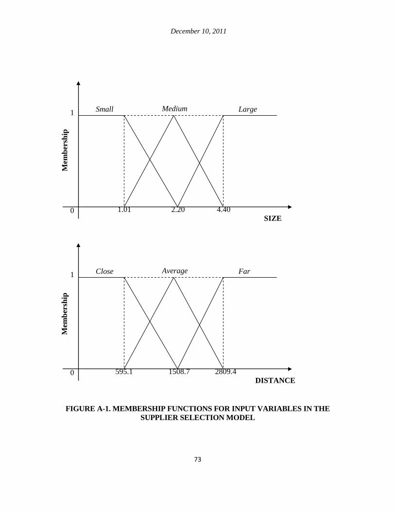
December 10, 2011
73
FIGURE A-1. MEMBERSHIP FUNCTIONS FOR INPUT VARIABLES IN THE SUPPLIER SELECTION MODEL
1.01 2.20 4.40 SIZE
Small Medium Large
0
1
595.1 1508.7 2809.4 DISTANCE
Close Average Far
0
1
Mem
bers
hip
Mem
bers
hip

December 10, 2011
74
TABLE A-1. DEFINITION FOR ESTABLISHMENT SIZE CLASSIFICATION
Establishment size category Range of number of employees 1 1 – 19 2 20 – 99 3 100 – 249 4 250 – 499 5 500 – 999 6 1000 – 2499 7 2500 – 4999 8 4999 <
3. INFERENCE METHOD
Inference engine is an essential component and core of a fuzzy logic system that
processes fuzzified input variables and provides the fuzzy output variable(s). All the rules in
this inference engine are simply expressed in linguistic form and are conceptually easy to
apprehend. The rules, however, may be extracted from a set of observed data or from expert
human experience. The latter is called fuzzy expert system and is very useful in the lack of
appropriate data. Similar to other modeling efforts, some sort of validation is required either
for the rules or the model outputs to assure the robustness of the model. Some rules were
defined based on the findings of other researchers (Altinoz, 2008; Stadtler, 2005; Choi and
Hartley, 1996; Spekman, 1988), and then all the rules were presented to more than 6,000
experts in the area of supply chain management in different industries for final evaluation.
They were asked in an online poll with around 2 percent response rate to score the
correctness of each rule on a scale of one to five. All the linguistic rules along with their
correctness score are presented in Table A-2.

December 10, 2011
75
TABLE A-2. LINGUISTIC RULES OF THE FUZZY RULE-BASED SUPPLIER SELECTION MODEL
Rule ID Linguistic From Score
1 If supplier and buyer are small, then partnership is unlikely. 2.4
2 If supplier is medium and buyer is small, then partnership is unlikely. 2.3
3 If supplier is small and buyer is medium, then partnership is unlikely. 2.3
4 If supplier is small and buyer is large, then partnership is average. 3.4
5 If supplier is large and buyer is small, then partnership is average. 3.4
6 If supplier and buyer are medium, then partnership is average. 3.8
7 If supplier is large and buyer is medium, then partnership is likely. 3.7
8 If supplier is medium and buyer is large, then partnership is likely. 3.7
9 If supplier is large and buyer is large, then partnership is likely. 3.5
10 If supplier and buyer are close, then partnership is likely. 3.9
11 If supplier and buyer are in average distance, then partnership is average. 3.7
12 If supplier and buyer are far, then partnership is unlikely. 3.0
In this case, the inference engine will evaluate all the rules for a given pair of supplier
and buyer and find the minimum degree of membership in each antecedent. This value will
be interpreted as the degree of membership in the consequent. Finally, fuzzy output could be
obtained by finding the maximum degree of membership for each category (unlikely,
average, and likely) of the output variable in the rule set. For example, four rules (1, 2, 3,
and 12) suggest membership values for the unlikely category of the output variable, but the
final membership value of the output variable would be the largest. Similar procedure
should be carried out to obtain membership values of the other two categories (likely and
average) of the output variable. Therefore, the output of this step of the model is a fuzzy
value for PARTNERSHIP for a given pair of supplier and buyer.
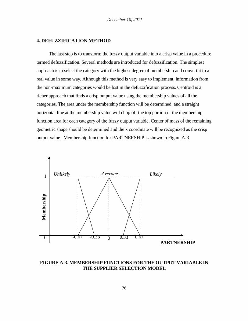
December 10, 2011
76
4. DEFUZZIFICATION METHOD
The last step is to transform the fuzzy output variable into a crisp value in a procedure
termed defuzzification. Several methods are introduced for defuzzification. The simplest
approach is to select the category with the highest degree of membership and convert it to a
real value in some way. Although this method is very easy to implement, information from
the non-maximum categories would be lost in the defuzzification process. Centroid is a
richer approach that finds a crisp output value using the membership values of all the
categories. The area under the membership function will be determined, and a straight
horizontal line at the membership value will chop off the top portion of the membership
function area for each category of the fuzzy output variable. Center of mass of the remaining
geometric shape should be determined and the x coordinate will be recognized as the crisp
output value. Membership function for PARTNERSHIP is shown in Figure A-3.
FIGURE A-3. MEMBERSHIP FUNCTIONS FOR THE OUTPUT VARIABLE IN THE SUPPLIER SELECTION MODEL
-0.67 0 0.67 PARTNERSHIP
Unlikely Average Likely
0
1
Mem
bers
hip
0.33 -0.33

December 10, 2011
77
APPENDIX B. SHIPMENT SIZE MODEL
1. INITIALIZATION
For each class of commodity and shipping distance category a matrix should be specified with three columns (small, average, and large). Number of rows in each matrix, however, is equal to the total number of supplier and buyer pairs with matching commodity type and shipping distance category. Array of the total annual tonnage of a known commodity type that the supplier is sending for the buyer in a specific distance category is also known. The ultimate goal of this model is to break down this array and determine share of small, average, and large shipments. These matrices are defined and initialized at this stage as explained in following:
a. Define sets of commodity types (C), shipping distance classes (D), and shipment size clusters (S). In this case: C = {1, 2, 3, …, 43}; D = {<50 miles, 50-99, 100-249, 250-499, 500-749, 750-999, 1000-1499, 1500-2000, >2000}; S = {<1000 lbs., 1000-50000, >50000 lbs.}
b. For each commodity type and shipping distance class , define
matrix with three (number of shipment size clusters) columns and R
rows, where R is the total number of supplier and buyer pairs that are trading commodity c and are at the distance of d.
c. For each row (r) in each that represents a specific pair of supplier and
buyer, calculate: i. F = Supplier’s establishment size
ii. T = Buyer’s establishment size iii. Ton = Annual tonnage of commodity c that is being traded between the
supplier and buyer iv. FS = Degree of membership of F in small category v. FM = Degree of membership of F in medium category
vi. FL = Degree of membership of F in large category vii. TS = Degree of membership of T in small category
viii. TM = Degree of membership of T in medium category ix. TL = Degree of membership of T in large category x. Small = (FS + TS) / FS + FM + FL + TS + TM + TL.
xi. Average = (FM + TM) / FS + FM + FL + TS + TM + TL. xii. Large = (FL + TL) / FS + FM + FL + TS + TM + TL.
xiii. Set: ° Small * Ton,

December 10, 2011
78
° Average * Ton,
° Large * Ton.
2. MODIFIED ITERATIVE PROPORTIONAL FITTING (IPF)
Initial values that are set in the first step are iteratively adjusted at this stage to obtain a relatively close match to the observed shipment size distribution in the Commodity Flow Survey. Sum of each row in a given matrix is given and should not be changed after redistributing shipment sizes. Share of small, average, and large shipments for a given commodity type and shipping distance cluster is known from 2002 Commodity Flow Survey, and therefore desired sum of each column could be easily obtained. Each cell of a given matrix could be estimated by an iterative proportional fitting approach, when sum of each row and sum of each column is given. The only restriction that should be considered in this iteration is that all the cells should be within the limits that are defined for the shipment size clusters. For instance, all the cells in the last common should be larger than 50,000, according to the definition of large shipments in this study. Similarly, all the cells in the second column should be larger than 10,000 but not necessarily smaller than 50,000. The latter is because each cell shows total weight of shipments that are in a specific cluster of shipment size and are traded between two known business establishments in a year. Following procedure should be carried out for each , after initialization to determine size of the shipments.
a. For each , set = tonnage share of commodity c, shipped in size
s at distance d, according to the Commodity Flow Survey data. For example = % 48 means % 48 of total tonnage of machinery products
(SCTG = 34) that was shipped less than 50 miles was medium size shipments, and the remaining 52% was either small of large, according to the Commodity Flow Survey data.
b. For each column (s), set Total_Column (s) = * sum of all the cells.
c. For each row (r), set Total_Row (r) = sum of the rth row. d. .
e. While , repeat the following:
i. Set ,

December 10, 2011
79
ii. Adjust each column: cell values in each column (j) are proportionally adjusted so they sum up to Total_Column (s). Shipment size limits should be observed in this step. If a cell has a value below the minimum limit (e.g. less than 50,000 in the third column) it should be adjusted so the conditions are not violated. The adjustment procedure is a straight forward heuristic:
° If a shipment is more than half but less than the minimum required weight of cluster definition, add the difference to it from the adjacent shipment size category.
° Larger shipment categories are in priority of giving. For example, if an average size shipment is 950 lbs. and is 50 lbs. below the minimum required of 1000 lbs., this 50 lbs. difference should first be considered to be obtained from large shipment category of the same row. However, if large shipment has a value less than 50050, this transfer would not be possible by definition, and then the small shipment size should be checked to obtain the difference.
° If a shipment is less than half of the required weight of cluster definition, this amount should be moved to the adjacent shipment size category.
° Larger shipment categories are in priority of receiving. iii. Adjust each row: cell values in each row (r) are proportionally adjusted so
they sum up to Total_Row (r). Shipment size limits should be observed similar to ii.
iv. Calculate
Although this approach is very straightforward and fully benefits from public data in the U.S., key information on shipment size determination is considered in this model. This includes establishment size of the supplier and buyer, shipping distance and commodity type. Since commodity type is defined at a considerably high resolution (2-digits Standard Classification of Transported Goods), this information embeds several characteristics of the commodity including value that significantly affects size of shipments. Contrary to the conventional iterative proportional fitting method with no control over the limits of the cell values, this approach could not exactly replicate the observed shipment size distribution in the Commodity Flow Survey data, because of the adjustments in steps ii and iii.

December 10, 2011
80
APPENDIX C. UIC NATIONAL FREIGHT SURVEY
Freight data is such a valuable piece of information that some firms are in the
business of collecting and analyzing it. Freight survey is always challenging because, as
mentioned earlier, the target population is reluctant to participate, and also the
information to be collected often include complex decisions that may be hierarchical
and/or interdependent. Furthermore, each contact is made under a severe time constraint,
since the respondents are typically surveyed while they are on the job. Thus, the survey
structure and methodology are particularly crucial in carrying out successful freight
surveys.
For this study, three survey methods were initially looked into, namely: mail-in
mail-out, telephone interview, and web-based. Since this survey targets a vast number of
business establishments across the U.S., in-person interview was rejected first. After
evaluating the expected response rates, costs, and convenience factors of each approach,
the web-based method was selected. Although a group of well-trained telephone
interviewers could obtain a high response rate, web-based method could be generally
performed in a more cost-effective manner and could take advantage of a variety of audio
and visual stimuli to enhance the survey questions (Couper et al., 2001). Furthermore,
web-based surveys can be completed at any time of the day by shipping managers who
tend to be very busy during office hours. Since web-based surveys, while more
economical than the telephone survey, tend to result in a low response rate that could
make the results fallible, some information must be obtained from non-participants in
order to assess the presence and the severity of the non-response bias (Heckman, 1990).
This will be discussed in more detail in this chapter.
1. SURVEY DEVELOPMENT
The main objective of this survey was to facilitate the development of the
proposed behavioral microsimulation of freight flow, Freight Activity Microsimulation

December 10, 2011
81
Estimator, in the U.S. Specifically, information on the modal selection process had to be
collected since such information was not available. An initial review of the freight
demand modeling studies, in addition to interviews with experts in the academia and
industry sectors were undertaken before and during the questionnaire design. Five basic
factors were found to have a significant impact on freight mode choice: accessibility,
reliability, cost, haul time, and flexibility. A preliminary version of the survey was
designed and later refined according to the inputs obtained from the knowledgeable
informants in the field of freight transportation and web-based survey design.
The survey had three major sections: relevant characteristics of the
establishments, information on five recent shipments, and contact information. Table C-1
summarizes the key questions in each section of the survey. A pilot survey was carried
out on January and February of 2009. The pilot was sent to around 1,200 randomly
selected business establishments and was followed by three follow-up emails, resulting in
a 1.0% participation rate. Although the response rate of 1.0% was anticipated for this
survey, some improvements in the final version of the survey caused a 20% increase in
the response rate.
A marketing company was hired to send recruiting emails on behalf of our
research team to randomly selected firms in the U.S. The responsibilities of the marketing
company were to provide a list of shipping managers or a person with the knowledge of
the shipping process in different industries; send an invitation email with an embedded
link to the survey on our behalf, which was already designed by our team; send the
reminders to the same population; and provide a follow up report when the survey was
finished.
The main survey was carried out in April and May of 2009 followed by three
email reminder that were sent 2, 7, and 14 days after the primary email contact,
respectively. Figure C-1 presents the trend of receiving completed questionnaires over
time. In total, 316 establishments participated in the survey providing information on 881
shipments across the country.

December 10, 2011
82
The follow up report contained some basic information about the firms in the
sampling frame, including participant’s name, phone number, address, company name,
industry classification, and employment size of the establishment. Also, this report
distinguished the persons who had opened the email and persons who had clicked on the
survey link. According to this report, over 4,000 of the initial emails which totaled more
than 30,000 bounced back. This made the number of successful email deliveries 25,997.
However, some emails, even though they did not bounce back, were filtered in the spam
folder of the recipients. The report revealed that, of the 25,997 establishments contacted,
a total of 4,544 recipients had successfully opened the emails. Around 9.3% of those
actually clicked on the survey link, but not all of them filled out the survey. To
investigate the effect of the spam filters, we randomly selected firms from the sampling
frame that was provided by the marketing company that carried out the recruiting, and
contacted them by phone and asked whether they had received the email in their mail box
or not. Roughly 40 persons were successfully contacted, of which less than half actually
received the email.
TABLE C-1. AN OVERVIEW OF SOME QUESTIONS IN THE UIC NATIONAL FREIGHT SURVEY
Section Question
I
Zip code of the establishment. Total gross floor area occupied by the establishment. Number of employees? Primary industry type of the establishment. Potential use of each mode of freight transportation by the firm. Access to rail-truck inter-modal facility. Warehousing situation in the company (owned / rented / outsourced).
II
Origin and destination. Mode(s) of transportation used for the shipment. Type, value, weight, and volume of the commodity. Cost and time of the entire shipping process. Whether the shipment was Inbound / Outbound / Import / Export / Containerized / Damaged / NOT delivered on time. Expected delivery time window at the destination. Use of consolidation center, distribution center, or warehouse for the shipment. Decision making unit (sending firm / receiving firm / a 3PL) Whether the same transportation mode was preferred TWO years ago for a similar shipment.
III Company name, address, phone, and email.

December 10, 2011
83
Respondent’s position in the company. Survey evaluation (Friendly / Neutral / Unfriendly) Willingness to participate in another online / telephonic / mail-in mail-out / in-person survey.
FIGURE C-1. TOTAL NUMBER OF PARTICIPANTS IN THE SURVEY OVER
TIME
2. DESCRIPTIVE STATISTICS
Once the survey was completed, the answers were downloaded from the survey
host site and cleaned. Respondents from a diverse range of industry type participated in
this survey. In terms of the geographical coverage, however, the survey collected inputs
from all the States except for Alaska, North Dakota, Utah, and Wyoming. On the other
hand, Illinois, Wisconsin, Montana, New Mexico, Nevada, New Hampshire,
Pennsylvania, and Nebraska had the highest participation rate. Since different industry
groups were invited to participate in the survey, information of a diverse range of
commodities was obtained. As illustrated in Figure C-2, mixed freight has the highest
share of 20%, while coal and minerals have a share of only 1%. With the data coverage
over a wide variety of commodity types, the demand model could be able to account for

December 10, 2011
84
commodity heterogeneity, which is an essential issue especially for a behavioral model.
Also, a rich dataset should cover a wide spectrum of shippers in terms of size. Fifty two
percent of the participants were from a company with an employee size of between 50
and 1,000, while 34% reported an employee size of less than 49, and the rest were large
firms with more than 1,000 employees.
Table C-2 shows the dollar value and weight of commodities that are shipped by
each mode of transportation. This table also compares the figures from this survey against
the 2002 Commodity Flow Survey (U.S. Department of Transportation, 2006). Share of
rail and truck are reasonably close in terms of value and weight of transported
commodities. However, air and water modes of transportation are somewhat skewed in
this survey and should be properly addressed in any analysis. Weighting the shipments in
a way that a decent match with the Commodity Flow Survey mode shares could be
obtained between aggregate shares of each mode is a simple solution. However, for the
ultimate objective of this study, which is the development of a behavioral mode choice
model, the data on air and water modes are not as critical as those for truck, rail, and
intermodal, because the mode choice for those two modes can be predicted rather
accurately based on the value and type of commodity being shipped. Also the behavioral
modal split model that is discussed in the following chapters has only focused on truck,
rail, and truck-rail intermodal.

December 10, 2011
85
FIGURE C-2. COMMODITY TYPES IN THE SURVEY.
TABLE C-2. VALUE AND WEIGHT SHARE OF EACH MODE IN THE
SURVEYED DATA
Mode Dollar Value Weight Shipments
COMMODITY FLOW
UIC2 COMMODITY FLOW
UIC UIC
Truck 68% 67% 60% 49% 69%
Rail 3% 4% 10% 12% 5%
Water 1% 8% 4% 8% 5%
Air, air & truck 5% 9% 0% 1% 11%
Intermodal3 15% 12% 7% 30% 11%
Pipeline & unknown 9% - 20% - - 1 Commodity Flow Survey (2002) data do not include imports and exports that pass through the United States from a foreign origin to a foreign destination by any mode. 2 UIC National Freight Survey. 3 Intermodal includes U.S. Postal Service and courier shipments and all intermodal combinations, except air and truck.

December 10, 2011
86
3. LESSONS LEARNED
The survey was successful in general and around 7% of the persons who opened
the recruiting email, filled out the questionnaire. However, following lessons could be
enlightening for future establishment surveys:
• Some critical characteristics must be known for all the businesses in the sampling frame to conduct the selection bias analysis. Otherwise collected data could be useless. Fortunately, such information can be obtained from various commercial sources at a reasonable price.
• Companies have to trust the survey team; otherwise they will not share their business information. Renowned and trustable logos could boost the response rate, while unrelated or infamous logos could have negative effects. According to the reviews that we got from some experts after the pilot, logo of a university research center was replaced by the logo of the University of Wisconsin at Madison, and a better response rate was obtained in the main survey.
• When conducting an online survey, spammed emails could be a very critical issue. A rough estimate of the number of spammed emails should be obtained in the pilot to make sure massive spamming problem will not occur in the main survey.
• Survey questions must be reviewed by experts, before and after the pilot. Categorical choices promote the respondents to answer a question, since the exact figures will not be revealed. In some cases, aggregation level could be left up to the respondents, by providing some options. This was practiced in this survey, when asking about the firm’s location and giving two choices of zip code and city.
• Some questions cannot be answered by the selected population and should be removed after the pilot to minimize the survey burden.
4. NON-RESPONSE BIAS ANALYSIS
Statistical analyses on a nonrandom sample can lead to questionable conclusions
and poor policies. If a survey is designed in a way that a group of population with
specific characteristics is more likely to be included in the sampling frame or participate,
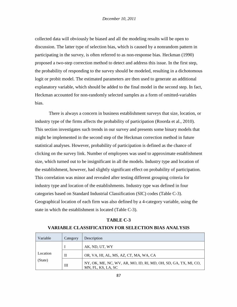
December 10, 2011
87
collected data will obviously be biased and all the modeling results will be open to
discussion. The latter type of selection bias, which is caused by a nonrandom pattern in
participating in the survey, is often referred to as non-response bias. Heckman (1990)
proposed a two-step correction method to detect and address this issue. In the first step,
the probability of responding to the survey should be modeled, resulting in a dichotomous
logit or probit model. The estimated parameters are then used to generate an additional
explanatory variable, which should be added to the final model in the second step. In fact,
Heckman accounted for non-randomly selected samples as a form of omitted-variables
bias.
There is always a concern in business establishment surveys that size, location, or
industry type of the firms affects the probability of participation (Roorda et al., 2010).
This section investigates such trends in our survey and presents some binary models that
might be implemented in the second step of the Heckman correction method in future
statistical analyses. However, probability of participation is defined as the chance of
clicking on the survey link. Number of employees was used to approximate establishment
size, which turned out to be insignificant in all the models. Industry type and location of
the establishment, however, had slightly significant effect on probability of participation.
This correlation was minor and revealed after testing different grouping criteria for
industry type and location of the establishments. Industry type was defined in four
categories based on Standard Industrial Classification (SIC) codes (Table C-3).
Geographical location of each firm was also defined by a 4-category variable, using the
state in which the establishment is located (Table C-3).
TABLE C-3 VARIABLE CLASSIFICATION FOR SELECTION BIAS ANALYSIS
Variable Category Description
Location
(State)
I AK, ND, UT, WY
II OR, VA, HI, AL, MS, AZ, CT, MA, WA, CA
III NY, OK, ME, NC, WV, AR, MO, ID, RI, MD, OH, SD, GA, TX, MI, CO, MN, FL, KS, LA, SC

December 10, 2011
88
IV TN, IN, NJ, VT, IA, DC, DE, KY, WI, PA, NE, NH, NV, IL, NM, MT
Industry Type
(SIC)
I 8, 9, 10, 12, 21, 29, 31, 43, 44, 53, 60, 61, 62, 63, 64, 76, 82, 83, 84, 86, 89
II 7, 13, 15, 16, 17, 20, 23, 25, 26, 32, 33, 37, 38, 41, 47, 48, 49, 50, 51, 52, 54, 55, 56, 65, 72, 73, 78, 79, 81
III 22, 24, 27, 28, 30, 34, 35, 36, 39, 45, 46, 57, 58, 59, 70, 80, 87
IV 1, 2, 14, 40, 42, 67, 75
Location, establishment size, and industry type of the recipients were inputted to
Limdep Econometric Software (Greene, 2002) to estimate the probability of participation
in the survey with logit and probit models. Newey and McFadden (1994) have more
details on discrete choice models. Final models are reported in Table C-4, with standard
t-values in the parentheses below each coefficient. Except for employment size, which
does not have any significant correlation with probability of participation, all other
coefficients are statistically significant with a 99 percent confidence interval. Neyman-
Pearson tests (Wald, Likelihood Ratio, and Lagrange Multiplier) were also performed to
see whether or not each model has a statistically significant explanatory power (Greene,
2002). Coefficient estimates and some model fit measures are summarized in Table C-4.
Model 1 estimates probability of participation among 4,544 recipients, who had opened
the email. However, the second set of models (Model 2) estimates such probability for
the entire population. A brief comparison between the first and second sets of models
does not show large fluctuations in coefficients of similar variables. Nonetheless, the first
set of models has a superior overall fit, which was expected. This is because the first set
of models are predicting a rare event with almost 9.3% chance of occurrence, while the
other set has only a chance of 1.6%.
The next stage is to choose between the logit and probit models. According to
most standard econometric textbooks, there is not a robust theoretical reason for
preferring logit over probit or vice-versa (Gujarati, 2003). However, very different
probabilities could be estimated by two binary choice models when modeling a rare event
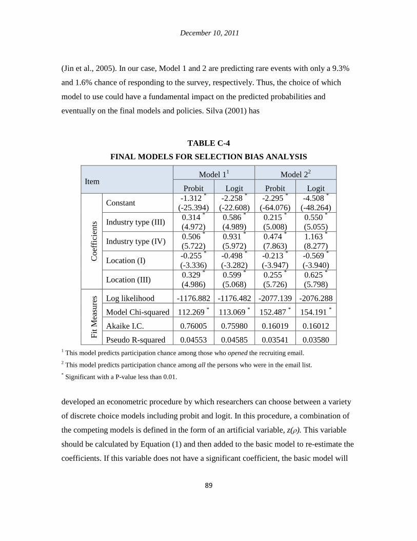
December 10, 2011
89
(Jin et al., 2005). In our case, Model 1 and 2 are predicting rare events with only a 9.3%
and 1.6% chance of responding to the survey, respectively. Thus, the choice of which
model to use could have a fundamental impact on the predicted probabilities and
eventually on the final models and policies. Silva (2001) has
TABLE C-4 FINAL MODELS FOR SELECTION BIAS ANALYSIS
Item Model 11 Model 22
Probit Logit Probit Logit
Coe
ffic
ient
s
Constant -1.312 * (-25.394)
-2.258 * (-22.608)
-2.295 * (-64.076)
-4.508 * (-48.264)
Industry type (III) 0.314 * (4.972)
0.586 * (4.989)
0.215 * (5.008)
0.550 * (5.055)
Industry type (IV) 0.506 * (5.722)
0.931 * (5.972)
0.474 * (7.863)
1.163 * (8.277)
Location (I) -0.255 * (-3.336)
-0.498 * (-3.282)
-0.213 * (-3.947)
-0.569 * (-3.940)
Location (III) 0.329 * (4.986)
0.599 * (5.068)
0.255 * (5.726)
0.625 * (5.798)
Fit M
easu
res Log likelihood -1176.882 -1176.482 -2077.139 -2076.288
Model Chi-squared 112.269 * 113.069 * 152.487 * 154.191 *
Akaike I.C. 0.76005 0.75980 0.16019 0.16012
Pseudo R-squared 0.04553 0.04585 0.03541 0.03580 1 This model predicts participation chance among those who opened the recruiting email. 2 This model predicts participation chance among all the persons who were in the email list. * Significant with a P-value less than 0.01.
developed an econometric procedure by which researchers can choose between a variety
of discrete choice models including probit and logit. In this procedure, a combination of
the competing models is defined in the form of an artificial variable, z(ρ). This variable
should be calculated by Equation (1) and then added to the basic model to re-estimate the
coefficients. If this variable does not have a significant coefficient, the basic model will

December 10, 2011
90
be preferred. In this case, logit model is set as the basic model, and z(ρ) is calculated for
three different values of ρ, according to Silva’s suggestion.
(1)
In the equation above, Pl and Pp are predicted probabilities by logit (basic model) and
probit models, respectively. is the derivative of the logistic function in the logit model
with respect to its utility function. An over-rejection trend of the null hypothesis was
revealed in a simulation analysis, which leads to a slight modification. Silva (2001)
suggested a weighted version of z, computed as in Equation (2).
(2)
As presented in Table VII, both weighted and non-weighted tests rejected the null
hypothesis with a more than 99 percent confidence interval, for all levels of ρ. Thus the
logit model is preferred to the probit. This model is could be used in the first stage of
Heckman correction (Heckman, 1990) for any further modeling effort on the surveyed
data. However, as pointed earlier in Table C-4, this model has a pseudo R-squared of
only four percent which is comparatively low and shows a very slight selection bias. In
the second stage, however, a transformation of these predicted probabilities (Heckman,
1990) should be added to each model as an extra explanatory variable to correct for this
slight bias.
TABLE C-5. SILVA TEST RESULTS FOR SELECTION BIAS ANALYSIS: LOGIT VERSUS PROBIT
Item Model 11 Model 22
Non-weighted Weighted Non-weighted Weighted
ρ = 0 1.27 (0.26)
1.77 (0.18)
3.21 (0.07)
3.47 (0.06)
ρ = 0.5 1.27 (0.26)
1.77 (0.18)
3.23 (0.07)
3.49 (0.06)
ρ = 1 1.27 (0.26)
1.78 (0.18)
3.24 (0.07)
3.50 (0.06)
1 This model predicts participation chance among those who opened the recruiting email.

December 10, 2011
91
2 This model predicts participation chance among all the persons who were in the email list. Note: P-values are reported in the parentheses.