Composable Models for Simulation-Based Design

Christiaan J. J. Paredis, Antonio Diaz-Calderon,

Rajarishi Sinha, and Pradeep K. Khosla

04-21-00

1

Composable Models for Simulation-Based Design

Christiaan J. J. Paredis, Antonio Diaz-Calderon, Rajarishi Sinha, Pradeep K. Khosla

Carnegie Mellon University Institute for Complex Engineered Systems

Department of Electrical and Computer Engineering Pittsburgh, PA 15213

{cjp, adiaz, rsinha, pkk}@cs.cmu.edu Abstract

This article introduces the concept of combining both form (CAD models) and behavior (simulation models) of mechatronic system components into component objects. By composing these component objects, designers automatically create a virtual prototype of the system they are designing. This virtual prototype, in turn, can provide immediate feedback about design decisions by evaluating whether the functional requirements are met in simulation.

To achieve the composition of behavioral models, we introduce a port-based modeling paradigm in which components interactions are defined by connections between ports. The port-based models are reconfigurable, so that the same physical component can be simulated at multiple levels of detail without having to modify the system-level model description. This allows the virtual prototype to evolve during the design process and to achieve the accuracy required for the simulation experiments at each design stage.

To maintain the consistency between the form and behavior of component objects, we introduce parametric relations between these two descriptions. In addition, we develop algorithms that determine the type and parameter values of the interaction models; these models depend on the form of both components that are interacting.

Our composable simulation environment has been implemented as a distributed system in Java and C++, enabling multiple users to collaborate on the design of a single system. We illustrate its functionality and use with a design scenario.

1 Introduction and Motivation

Because of the intense competition in the current global economy, successful companies must react quickly to changing trends in the market place. For example, the need for a new product can be triggered by the introduction of new technologies, changes in

customer demands, or fluctuations in the cost of basic materials and commodities. To capitalize on these imbalances in the market, a company must conceive, design, and manufacture new products quickly and inexpensively. Because the design process consumes a significant portion of the total development time, a shorter design cycle provides a distinct competitive advantage.

The design cycle can be shortened significantly through virtual prototyping. A virtual prototype enables the designers to test whether the design specifications are met by performing simulations rather than physical experiments; a physical prototype is only needed for final testing. Not only does virtual prototyping make design verification faster and less expensive, it provides the designer with immediate feedback on design decisions. This in turn promises a more comprehensive exploration of design alternatives and a better performing final design. To fully exploit the advantages of virtual prototyping, however, simulation models have to be accurate and easy to create.

Virtual prototypes need to model the behavior of the equivalent physical prototype accurately; otherwise, the predicted behavior does not match the actual behavior resulting in poor design decisions. But creating accurate models is a hard problem. Only recently has computing performance reached a level where high fidelity simulation models are economically viable. For instance, it is now feasible to evaluate dynamic simulations of finite element models for crack propagation. However, not always are the most detailed and accurate simulation models also the most appropriate; sometimes it is more important to evaluate many different alternatives quickly with only coarse, high-level models. For instance, at the early stages of the design process, detailed models are often unnecessary because many of the design details still have to be decided and accurate parameter values are still unknown. At this stage, the accuracy of the simulation result depends more on the accuracy of the parameter values than on the model equations; simple equations that describe

2

the high-level behavior of the system are then most appropriate.

Equally important to accuracy is the requirement that simulation models be easy to create. Creating high-fidelity simulation models is a complex activity that can be quite time-consuming. To take full advantage of virtual prototyping, it is necessary to develop a modeling paradigm that supports model reuse, that is integrated with the design environment, and that provides a simple and intuitive interface which requires a minimum of analysis expertise. This paper introduces such a paradigm, composable simulation, which is based on model composition from system components.

2 Composable Simulations

To provide better support for simulation-based design of mechatronic systems, we have developed a modeling and design paradigm based on composition. A wide variety of products, ranging from consumer electronics to cars, contain mostly off-the-shelve components and components reused from previous design generations; for instance, in cars, the portion of completely new components is often less than twenty percent. As a result, the design of such systems consists primarily of the configuration or assembly of existing components.

The modeling of such systems can also be viewed as composition. We can obtain a system level simulation model, by combining the component models with the models that define the interactions between the components. Assuming that the models for individual components already exist in a component library, and that the physics of the interactions between the components have been modeled in a library of interaction models, a system level simulation model can be generated through the composition of existing component and interaction models.

To take advantage of the parallelism between the design and modeling activities—both consist of the composition of system components—we have developed a modeling and design framework in which the form and the behavior of a component are combined into a single component object. By composing component objects into systems, a designer simultaneously designs and models new artifacts. This is already common practice in electrical CAD software; when creating a chip layout, the instantiation of a transistor or logic gate creates the geometry for the silicon layers as well as the corresponding simulation model.

In mechanical CAD, the integration between design and simulation is not as common. For purely

mechanical systems, most commercial CAD packages do provide an optional module for multi-body simulation, but these modules lack sufficient support for multi-disciplinary systems.

Our goal is to extend this design paradigm to multidisciplinary systems, specifically mechatronic systems. The traditional design approach for multidisciplinary systems has been a sequential design-by-discipline approach: First design the mechanical system, than the sensors and actuators, and finally the control system (Shetty and Kolk 1997). This approach imposes artificial constraints by fixing the design at various points in the design sequence. In mechatronic design, on the other hand, synergy between the different disciplines is achieved by designing all disciplines concurrently. To evaluate whether a mechatronic design prototype meets the design specifications, the designer must consider the component interactions in all energy domains. This would be prohibitively expensive without the intensive use of simulation.

Existing simulation tools for multidisciplinary systems are very general, stand-alone tools that are not integrated with the design environment. The main goal of the simulation and design environment that we have developed is to support multidisciplinary simulation-based design within an integrated software environment. Specifically, the framework has the following characteristics, which we will address in detail in the subsequent sections:

A port-based modeling paradigm: To take advantage of the compositional nature of both design and modeling of mechatronic systems, we have developed a port-based modeling paradigm in which the user can compose system-level simulations from component models. By connecting the ports of the subcomponents, the user defines the interactions between them. In Section 4, we will describe the port-based modeling paradigm in more detail.

Reconfigurable Models: At each stage of the design process, the designer performs different simulation experiments to verify whether the design prototype meets the functional requirements. In the early, conceptual stage, these experiments may include quick trade-off analyses that require limited accuracy, while towards the end of the detailed design stage, the designer may decide to perform a comprehensive, detailed simulation. To accommodate simulations at different levels of detail without the need for remodeling the complete system, we develop the concept of reconfigurable models in Section 5. These models can evolve with the design prototype throughout the design process.

Simulation integrated with CAD: The building blocks in our simulation and design environment are

3

component objects; they describe both the form and the behavior of system components. In Section 6, we describe how the CAD description of the form may be used to extract the lumped parameters of the behavioral models. In addition, we have developed algorithms that instantiate models of mechanical interactions based on the form of the interacting components.

A component library: The component objects are organized in a hierarchical component library. From this library, the designer selects the components that achieve the desired functionality within the system. We provide a detailed description of the component library and its implementation in Section 7.

3 Related Work

3.1 Modeling and Simulation There exist already many modeling paradigms and

commercial simulation packages. They can be characterized according to the following criteria: graph-based versus language-based, multi-domain versus single-domain, and declarative versus procedural modeling.

The best known of the graph-based modeling paradigms is Bond Graph modeling (Dixhoorn 1980; Karnopp et al. 1990; Painter 1961; Rosenberg and Karnopp 1983). It is based on energy-conserving junctions that connect energy storing or transforming elements with bonds; the bonds represent the energy flow between the modeling elements. Bond graph modeling has the advantage that it is domain independent and based on energy flow, but it is not very convenient for the modeling of 3D mechanics or continuous-discrete hybrid systems. Furthermore, beginning users find it counterintuitive that the topology of a bond graph is different from the topology of the corresponding physical system.

Linear graph models do reflect the system topology directly (Branin 1966; Trent 1955). They are also domain independent and can be easily extended to model 3D mechanics (Andrews et al. 1988; McPhee 1996; Richard et al. 1995) and hybrid systems (Muegge 1996; Roe 1966). The VHDL-AMS language, which we use for modeling, builds on the concepts of linear graph modeling, although it does not require an explicit graph representation (Christen et al. 1999; IEEE 1999).

The majority of modeling paradigms is not graph-based, but language-based. A large number of modeling languages are derived from the CSSL (continuous system simulation language) standard developed by the Technical Committee of the Society for Computer Simulation (Strauss and and others

1967). These languages have in common that they are procedural. A model is defined by a procedure that computes the derivatives of the state for a given state and time. A second group of modeling languages is equation-based or declarative: Modelica (Elmqvist et al. 1998), Easy5 (The Boeing Company 1999), Dymola (Dynasim AB 1999), Omola (Anderson 1994), and VHDL-AMS (IEEE 1999). Here the model is defined by a set of equations that establishes relations between the states, their derivatives, and time. The simulation engine is responsible for converting these equations into a software expression that can be evaluated by the computer. The advantage of declarative languages is that the user does not have to define the mathematical causality of the equations, so that the same model can be used for any causality imposed by other system components.

Many of the declarative languages are also object-oriented and support multiple energy domains. This is the case for VHDL-AMS, the language that we use. VHDL-AMS has the additional advantage that it supports both continuous time and discrete time systems.

3.2 Simulation-based Design Many companies are resorting to simulation tools

to improve their design process. A well-publicized example of virtual prototyping is the design of the Boeing 777 airplane. Boeing switched from a paper-based design process to a fully digital representation, allowing them to perform performance analysis (using CFD software) and assemblability analysis without the need for building physical prototypes. This resulted in a significantly shorter design and testing period. A similar all-digital approach is also being adopted by car manufacturers.

Although the success of simulation-based design has already been demonstrated commercially, many unresolved research issues remain to be addressed. Ongoing research includes model validation, automatic meshing and model creation, integration of simulation engines in different domains, architectures for collaboration, and visualization using virtual reality technology. In this paper, we focus on simplifying the process of model creation, by integrating form and behavior into component objects.

Our approach is based on the characterization of a design prototype by its form, function, and behavior (Pahl and Beitz 1996). The form is a description of the physical embodiment of an artifact, while function is the purpose of the artifact—the behavior that the designer intended to achieve. As is illustrated in Figure 1, the actual behavior does not

4

depend on the function, but only on the form. During design or synthesis, we transform function into form, while, during design verification, we derive the behavior from the form and verify whether this behavior matches the function. In the context of virtual prototyping, the behavior is described by mathematical models and design verification is achieved by performing simulation experiments with these models.

The design process is iterative and hierarchical in nature. To solve complex design problems, a design team typically considers the problem at different levels of abstraction, ranging from very high-level system decompositions to very low-level detailed specification of components (Keirouz et al. 2000; Vries and Breunese 1995). During this process, the design team adds information and thus transforms the design representations. For instance, a needs assessment is transformed into design specifications and engineering requirements; engineering requirements, in turn, are converted into a family of solutions that are evaluated and compared (possibly using simulation) to iterate on the description of the artifact in terms of form, function, and behavior (Pahl and Beitz 1996). As a result, all representations evolve simultaneously from the initial high-level decompositions to increasingly detailed descriptions of the design artifact.

In the early stages of the design process, when only few physical details have been defined, simulation models can capture the function or intended behavior of sub-systems, allowing one to use simulation to make important conceptual trade-offs. As more details of the actual embodiment or form are included in design artifacts, the expected behavior of the sub-systems can be replaced gradually by the actual behavioral models of the physical components. The modularity of our port-based modeling paradigm facilitates these model substitutions just as it provides a basis for reconfigurable models.

4 Port-Based Modeling Paradigm

To achieve composability of behavioral models, we have developed a port-based modeling paradigm. This paradigm is based on two concepts: ports and connections (Diaz-Calderon et al. 2000a; Diaz-Calderon et al. 2000b).

Ports correspond to the points where a component exchanges energy with the environment. All energy is exchanged through ports. There is one port for each separate interaction point, and the type of a port matches the type of the energy exchange. For example, a DC motor has four ports, two electrical and two mechanical. The electrical ports correspond to the electrical connectors of the motor, the mechanical ports to the stator and the rotor—one port for each rigid body.

The energy flow through a port is characterized by an across and a through variable, also called effort and flow variables in Bond Graph modeling (Painter 1961; Rosenberg and Karnopp 1983). Examples of across variables are voltage in the electrical domain and velocity in the mechanical domain. They are measured across the port relative to a global reference. The corresponding through variables, electrical current and mechanical force, are measured through the port.

The interactions between components are represented by connections between ports. Each connection imposes algebraic constraints on the port variables. These constraints are the equivalents of the Kirchoff voltage and current laws in electrical circuits. One type of constraint requires that the across variables be equal, the other that the sum of the through variables be zero.

As a reflection of the underlying physics, both connections and ports are undirected. An electrical resistor does not have an input and an output; the energy through its ports can flow in either direction. In mathematical terms, this requires that the components and connections be modeled as declarative equations rather than assignments. Many recent simulation languages are declarative, including Modelica, VHDL-AMS, and Dymola; SimuLink, on the other hand, is procedural. When solving a set of declarative differential equations, the solver must first determine the mathematical causality of the equations. For this purpose, we have developed an algorithm based on a minimum cost spanning tree algorithm (Diaz-Calderon et al. 2000a).

All the ports combined form the interface of the model. This interface defines how the component can interact with the other components in the system, but does not contain any information about the internal behavior of the component. Instead, the

FormSynthesis Modeling

BehaviorFunction

Analysis

FormSynthesis Modeling

BehaviorFunction

Analysis

Figure 1: Relation between form, function, and behavior in the context of virtual prototyping.

5

interface encapsulates the implementation of the model, which defines the internal behavior of the component

As illustrated in Figure 2, a port-based model can be hierarchically defined when it consists of a composition of sub-models, resulting in a compound component. When the sub-models are also compound, multiple levels of hierarchy occur. The bottom of the hierarchy must consist of primitive models that are defined only by their constitutive equations.

The constitutive equations relate all the across and through variables of a component model. For exam-ple, the constitutive equation for a resistor relates the voltage difference between the two ports with the current through the ports according to Ohm’s law. Since the model is declarative, the solver may instantiate this single equation either as RIV or

RVI / , depending on how the resistor is used in the circuit. In general, the model equations may include a combination of both algebraic and ordinary differential equations.

In addition to ports and connections that model energy flow, we also consider signal connections and signal ports. No energy flows through signal ports,

and the connections between them are directed. This reflects the physics of a low-impedance electrical output driving a high-impedance input; the signal can only flow from the output to the input, an operation that requires almost no power. Examples of systems with signals are computer networks, data buses, or embedded controllers; they can be modeled as block diagrams similar to SimuLink models. Signal components are defined by procedures rather than constitutive equations. Since the mathematical causality of a procedure is fixed (inputs are independent, and outputs are dependent variables), special care needs to be taken when solving hybrid systems. Hybrid systems contain both energy-based and signal components, as in most mechatronic systems.

The port-based modeling paradigm cannot be applied to all systems; it is limited to systems with lumped interactions. When an interaction is distributed in nature, as between a boat and the water on which it floats, it must be approximated by a large number of lumped interactions. The internal model of a component, however, may still be distributed. Consider, for example, a flexible beam attached to a structure by its two ends. A finite element model may describe the internal behavior of the beam, but the interaction with the structure can still be captured with only two ports. For mechatronic systems, the primary interactions between components tend to be lumped, so that the port-based modeling paradigm is applicable. Only when very detailed models are required, may we have to consider phenomena, such as thermal interactions, that are distributed in nature.

We have implemented the port-based modeling approach for the electrical, mechanical, and signal domains (Diaz-Calderon et al. 1999; Sinha et al. 2000).

5 Reconfigurable Models

Most object-oriented modeling languages have a concept similar to ports (sometimes called terminals, or connectors) (Anderson 1994; Elmqvist et al. 1998; IEEE 1999; Sahlin 1996), and it is possible to use these languages to describe the composable and hierarchical port-based models introduced in the previous section. However, these languages do not guarantee a clear separation between the interface of the model and the implementation of its behavior, often merging both concepts into a single modeling object. To create models that can evolve with the design, we need the capability to bind different implementations to the same interface, allowing the designer to select a more detailed behavior for a component, without having to remodel its interactions with the rest of the system.

C om plex sys tem

Prim itive system

In terface

System E

systemC

systemD

systemB

systemA

systemB

systemC

a

b

c

d e f

d

constitutiveequations

param eters

param eters

param eters

ports

parameterrela tion

parameterpropagationchannel

N on-causa l connection

C ausa l connection

Figure 2: Port-based simulation models may be

hierarchically defined.

6

In traditional object-oriented modeling languages, the behavior of a model can only be modified by changing the values of the parameters. In our approach, the structure of the model can be modified also, resulting in reconfigurable models. In a reconfigurable model, the interface of the model and the implementation of its behavior are considered two separate concepts. As is illustrated in Figure 3, each implementation has a corresponding interface, but a single interface may have multiple implementations associated with it.

In the definition of reconfigurable models, we consider two principles: composition and instantiation.

Through the principle of composition, a model implementation can be defined as a set of interfaces of sub-components and the interactions between them, as in implementation A in Figure 3. At this point, the sub-components do not yet have any behavior; they are represented only by their interface. This allows us to define the interactions between sub-components independently of their internal behavior. One can think of an interface as the equivalent of an abstract class in object oriented programming; it defines the methods through which one can interact with the object, but it does not provide an implementation.

An abstract model becomes concrete by instantiating an implementation. Only implementations that match the interface can be instantiated. Moreover, the semantics of the implementation must match the semantics of the interface. For example, the interface of an electrical resistor has the same ports as the interface of a capacitor. However, because the semantics of the two components are different, only resistor

implementations can be instantiated for a resistor interface.

Like general port-based models, reconfigurable models can be hierarchical. Because compound implementations are a composition of abstract interfaces, they themselves are also abstract. The instantiation of a compound model, therefore, requires the recursive instantiation of all the interfaces of its subcomponents. The number of possible configurations of a compound model can grow very large when considering all possible combinations of implementation bindings. We call this set the model space of the component. The advantage of reconfigurable models is that all the elements of the model space can be instantiated without having to redefine the interactions with other system components, because the interface remains the same.

The instantiation principle also allows the definition of families of components. In this case, the implementations for an interface do not represent different behavioral models for a single component, but instead represent models for a family of components that all share the same interface. For example, a family of DC motors may all share an interface consisting of two mechanical and two electrical ports. When designing a system, the designer can include this interface in the system model without having to select a particular DC motor. It may be possible to select the most appropriate DC motor, by performing a series of simulation experiments each with a different motor from the family; each new experiment only requires that a new implementation be bound to the DC motor interface.

As is illustrated in Figure 4, the complete set of implementations for an interface can be represented as an AND-OR tree. The structure of the AND-OR

param eters

System E

constitu tiveequations

im p lem enta tion C

im p lem enta tion B

im p lem enta tion A

Figure 3: A reconfigurable model consisting of an

interface and three implementations.

BothInductanceResistance

Loss FreePower Conversion

Electro-Mech.Implementation

Implementationn

DC motor

ConversionElectrical Mechanical

Ideal Model Armature Losses

Friction No Friction

OR OR

OROR

AND AND

AND AND Interface

ImplementationBothInductanceResistance

Loss FreePower Conversion

Electro-Mech.Implementation

Implementationn

DC motor

ConversionElectrical Mechanical

Ideal Model Armature Losses

Friction No Friction

OR OROR OR

OROR OROR

AND ANDAND AND

AND ANDAND AND Interface

Implementation

Interface

Implementation

Figure 4: An AND-OR tree representation of a

reconfigurable model.

7

tree and the principles of composition and instantiation are closely related. AND arcs point from an implementation to the interfaces from which it is composed. Similarly, OR arcs point from an interface to the implementations from which it can be instantiated. For example, the AND-OR tree in Figure 4 depicts a DC-motor model. The top-level interface has three different implementations associated with it, represented by three OR arcs. The electro-mechanical model implementation has three AND arcs, meaning that it is a compound model consisting of three interfaces: electrical, conversion, and mechanical. When instantiating a particular model in the model space, we must bind implementations to interfaces. Working our way down from the top to the bottom of the AND-OR tree, we must first assign an in implementation to the top-level interface and then recursively to each of the interfaces that constitute the selected implementations.

6 Relation between Behavior and Form

Composable simulations are based on the concept of component objects that combine form and behavior. By composing component objects into systems, a designer simultaneously designs and models new artifacts. The previous two sections introduced a modular modeling paradigm that supports such composition. In this section, we focus on guaranteeing that these behavioral models are consistent with the corresponding form descriptions as represented by a CAD model.

We distinguish between two different types of behavioral models: models representing physical components, and models representing interactions between components. Examples of physical components are motors, screws, shafts, or controllers. Their component objects contain a description of both form and behavior. Interaction models, on the other hand, do not have any associated form. Yet, their model parameters can be extracted from the form of the two interacting components. Examples of interaction models are lower pairs that result from mechanical contact, contact resistance in an electrical switch, or magnetic forces between two magnets.

6.1 Form and Behavior of Component Objects

A component object contains a description of the form of the component as well as a reconfigurable model describing its behavior. The reconfigurable model may describe the component at different levels of abstraction or with respect to different energy domains, and provides, in this way, different views of the component. These views share one common

aspect: they are all behavioral descriptions of the same form.

Ideally, behavioral models are generated from the form automatically. This requires combining information about geometry and materials with knowledge of the physical phenomena occurring in the component. Creating such models automatically is too difficult in the general case, but can be achieved for certain classes or families of components. For example, the mechanical behavior of the set of rigid bodies with homogeneous material properties is completely defined by the mass and inertial parameters, as is shown in Figure 5. These rigid bodies are so common in mechatronic systems, that it makes sense to develop a procedure that computes the inertial parameters from the density and the geometry of the component, as defined in a CAD model. As a result, the behavior models of homogeneous rigid bodies can be derived automatically for any material and arbitrary geometry.

Besides rigid bodies, we can automatically generate behavioral models for parametric models. In a parametric CAD model, the designer establishes relationships between certain geometric dimensions or parameters. As a result, the form is completely defined by a limited set of characteristic parameters or features. Behavioral models also contain parameters, which, in turn, can be related to the CAD parameters. These relations can be simple, as in the rigid body example, or can be quite complicated, as for a hydraulic pipe. As is illustrated in Figure 5, the flow resistance of the pipe depends on its length, diameter, and bending radii. Although these dimensions may not be defined explicitly in the CAD model, they can be extracted through parametric relations captured as procedures (Bettig et al. 2000; Shah and Mantyla 1995).

Mass, Center of Gravity

Inertia Tensor

Component Model

ZZD IIM

xmF

u�

¦

¦ ��

Pipe diameter

Pipe shape

Pipe Model

Flow Resistance =F(L, R1, R2, D, …)

R1

R2

D

L

MicroMo XYZ DC-Motor

Parameters = Lookup(XYZ)

Mass, Center of Gravity

Inertia Tensor

Component Model

ZZD IIM

xmF

u�

¦

¦ ��

Pipe diameter

Pipe shape

Pipe Model

Flow Resistance =F(L, R1, R2, D, …)

R1

R2

D

L R1

R2

DD

L

MicroMo XYZ DC-Motor

Parameters = Lookup(XYZ)

Figure 5: The relation between form and behavior parameters.

8

Finally, one can consider the case in which both geometric and behavioral parameters are determined through a lookup table. For instance, given the model type of a DC motor, a lookup table provides all the parameters for a detailed behavioral model. Similarly, a parametric CAD model is instantiated from parameter values in the lookup table. What makes this example significantly different from the previous example is that there may not be any direct relation between the geometric parameters and the behavioral parameters. The geometry may simply be a high-level abstraction of the DC-motor, capturing only the external geometry through which the motor can interact with other components. These simplified geometric representations of the form no longer contain any relevant information from which an internal behavioral model can be extracted.

6.2 Form and Behavior of Component Interactions

In addition to the behavioral models of component objects, systems include models describing the interactions between component objects. For each pair of interacting component objects, there is an interaction model that relates the port variables of the two objects to each other.

Any interaction in any energy domain requires an interaction model. However, for the electrical domain, the interaction model is usually very simple. An electrical connection between two components is modeled sufficiently accurately by constraining the voltage at the two connecting ports to be equal and the current through them to add to zero. Because this interaction model is so common, we allow it to be omitted in our modeling paradigm, as is shown in Figure 6. In the mechanical domain, the equivalent default model is rarely appropriate. Even when connecting two components rigidly, their reference frame is usually in a different location so that a model representing the coordinate transformation is needed.

Besides rigid connections, other common

mechanical interaction models are the lower pair kinematic constraints. We have developed algorithms to extract the type and parameters of a lower pair from the geometry of the interacting components (Sinha et al. 1998; Sinha et al. 2000).

Previously, kinematic analysis was limited to parts with only planar faces (Mattikali et al. 1994). Since most engineering devices contain curved surfaces, these analyses either did not apply or failed to recognize certain degrees of freedom when approximating the curved faces with polygonal facets.

In our work (Sinha et al. 1998; Sinha et al. 2000), we have extended these results to curved contacts, as is shown in Figure 7. When two rigid parts share a surface-to-surface contact, every contact point is subject to a non-penetration condition. This condition requires that the instantaneous velocity between the two bodies does not have a component in the direction opposite to the surface normal at the contact point. We write this condition as a linear inequality of the form:

0)( txu� nrv&&&&

Z , (1)

where v&

and Z&

are the relative translational and angular velocities between the two bodies, r

&

is the position of the point, and n

&

is the normal to the contact surface. Imposing Equation (1) at every point on the contact surface is equivalent to imposing the constraint at the vertices of the convex hull. Therefore, the analysis results in a linear relationship of the form:

0t»¼

º«¬

ª

Z

&

&

vJassembly , (2)

where each row of Jassembly represents a non-penetration constraint, as in Equation (1). From the

PhysicalObject A

PhysicalObject B

Interaction Model

Interaction Model

Mechanical Domain(complex interaction)Mechanical Domain(complex interaction)

Joint Model, Gear Model, Friction.

Electrical Domain(default interaction)Electrical Domain(default interaction)

BA acrossacross

0throughi

¦

ComponentA

ComponentB

Node ComponentA

ComponentB

InteractionComponent

PhysicalObject A

PhysicalObject B

Interaction Model

Interaction Model

Mechanical Domain(complex interaction)Mechanical Domain(complex interaction)

Joint Model, Gear Model, Friction.

Electrical Domain(default interaction)Electrical Domain(default interaction)

BA acrossacross

0throughi

¦

BA acrossacross

0throughi

¦

ComponentA

ComponentB

Node ComponentA

ComponentB

InteractionComponent

Figure 6: Interactions between system

components.

3DUWLDO F\OLQGULFDOFRQWDFW ZLWK � SRLQWV

7ZR YLHZV RI D � SDUW DVVHPEO\

0

0025.025.0

252525.025.0

0025.025.0

252525.025.0

252525.025.0

0025.025.0

252525.025.0

0025.025.0

d

»»»»»

¼

º

«««««

¬

ª

»»»»»»»»»»»

¼

º

«««««««««««

¬

ª

�

�

�

���

��

���

�

y

x

y

x

v

v

Z

Znedunconstrai ,

0

zz

yxyx

v

vv

Z

ZZ

3DUWLDO F\OLQGULFDOFRQWDFW ZLWK � SRLQWV

7ZR YLHZV RI D � SDUW DVVHPEO\

0

0025.025.0

252525.025.0

0025.025.0

252525.025.0

252525.025.0

0025.025.0

252525.025.0

0025.025.0

d

»»»»»

¼

º

«««««

¬

ª

»»»»»»»»»»»

¼

º

«««««««««««

¬

ª

�

�

�

���

��

���

�

y

x

y

x

v

v

Z

Znedunconstrai ,

0

zz

yxyx

v

vv

Z

ZZ

Figure 7: Extracting the type and parameters for

lower pair interaction models.

9

properties of the Jassembly matrix, we can determine the kinematic constraints between two interacting component objects. For example, the basis vectors of the nullspace of Jassembly define the contact-preserving degrees of freedom.

Our method can infer behavior from devices with curved geometry, while at the same time resolving global, multi-part interactions. We have developed procedures that derive the Jassembly matrix directly from the CAD models, and from it determine the type and parameters of the interaction models (Sinha et al. 1998; Sinha et al. 2000).

7 Component Libraries

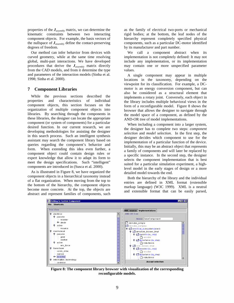
While the previous sections described the properties and characteristics of individual component objects, this section focuses on the organization of multiple component objects into libraries. By searching through the components in these libraries, the designer can locate the appropriate component (or system of components) for a particular desired function. In our current research, we are developing methodologies for assisting the designer in this search process. Such an intelligent synthesis assistant may search the component library based on queries regarding the component’s behavior and form. When extending this idea even further, a component object could contain design rules or expert knowledge that allow it to adapt its form to meet the design specifications. Such “intelligent” components are introduced in (Susca et al. 2000).

As is illustrated in Figure 8, we have organized the component objects in a hierarchical taxonomy instead of a flat organization. When moving from the top to the bottom of the hierarchy, the component objects become more concrete. At the top, the objects are abstract and represent families of components, such

as the family of electrical two-ports or mechanical rigid bodies; at the bottom, the leaf nodes of the hierarchy represent completely specified physical components, such as a particular DC-motor identified by its manufacturer and part number.

We call a component abstract when its implementation is not completely defined: It may not include any implementation, or its implementation may contain one or more unspecified parameter values.

A single component may appear in multiple locations in the taxonomy, depending on the viewpoint for its classification. For example, a DC-motor is an energy conversion component, but can also be considered as a structural element that implements a rotary joint. Conversely, each object in the library includes multiple behavioral views in the form of a reconfigurable model. Figure 8 shows the browser that allows the designer to navigate through the model space of a component, as defined by the AND-OR tree of model implementations.

When including a component into a larger system, the designer has to complete two steps: component selection and model selection. In the first step, the designer decides which component to use for the implementation of a particular function of the device. Initially, this may be an abstract object that represents a family of components and will later be replaced by a specific instance. In the second step, the designer selects the component implementation that is best suited for a particular simulation experiment, a high-level model in the early stages of design or a more detailed model towards the end.

Both the hierarchy of the library and the individual entries are defined in XML format (extensible markup language) (W3C 1999). XML is a neutral and extensible format that can be easily parsed,

Figure 8: The component library browser with visualization of the corresponding

reconfigurable models.

10

searched, and shared over the Web. Our XML representation for component objects includes pointers to geometric models (ACIS or Pro/E), an interface definition of the behavioral model, and pointers to the corresponding implementations.

The definition of an implementation is also stored in XML format. The equations tags in primitive implementations are based on the VHDL-AMS standard (IEEE 1999). The component descriptions may also contain meta-knowledge capturing the semantics of the model: What are the assumptions? When is the model valid? Or, what is the meaning of the model? We anticipate using this meta-knowledge extensively when searching for components based on their function.

8 Software Architecture and Implementation

The implementation architecture of our simulation-based design environment is similar to the Open Assembly Design Environment (OpenADE) developed at NIST (Keirouz et al. 2000). As is shown in Figure 9,the core of our system is a central design database in which the representations for the current design are stored: function, behavior, product structure, and CAD data. Furthermore, the database contains the relationships between these representations; for instance, if a system component implements a particular function, the database will contain a “has_function” relation pointing from the object to its functional model, and an “implemented_by” relation from the model to the object.

During the design process, the information in the central database is continually transformed by autonomous software agents or by the designer—through graphical user interfaces, shown in Figure 10.

The main interaction between the designer and the database occurs through the 3D CAD GUI and the behavior model GUI. The 3D CAD GUI is implemented using the Java3D toolkit. It allows the

DesignDatabase:

• Functional Model• Behavioral Model• Product Structure• CAD data• …

DesignDatabase:

• Functional Model• Behavioral Model• Product Structure• CAD data• …

CAD GUICAD GUI

Structure GUIStructure GUI

Function GUIFunction GUI

Behavior GUIBehavior GUI

Param. ExtractionParam. Extraction

Simulation EngineSimulation Engine

Data TranslatorData Translator

……

DesignDatabase:

• Functional Model• Behavioral Model• Product Structure• CAD data• …

DesignDatabase:

• Functional Model• Behavioral Model• Product Structure• CAD data• …

CAD GUICAD GUI

Structure GUIStructure GUI

Function GUIFunction GUI

Behavior GUIBehavior GUI

Param. ExtractionParam. Extraction

Simulation EngineSimulation Engine

Data TranslatorData Translator

…… Figure 9: Java-Based GUI components and services interact through a shared design

database.

3D CAD modeling

Component library

Behavior Modeling

Component editor

3D CAD modeling

Component library

Behavior Modeling

Component editor

Figure 10: CAD GUI and Behavioral Model GUI

11

user to view and manipulate the geometry associated with the system components, and to define mechanical interactions between components. It does not allow the geometry of individual components to be modified; that functionality will be provided in the future by integrating our framework with Pro/Engineer. The current Java-based 3D GUI will remain useful for system-level interactions that do not require the design of new components.

The behavioral modeler provides a 2D view of the system. Each of the system components appears in this view as a port-based model.

In addition to the user interfaces, software agents interact with the design repository. These agents can act as design assistants, working in the background. The tasks performed by such agents include the following:

x the translation of CAD data to VRML format for rendering,

x the extraction and verification of mechanical component interactions,

x the compilation of behavioral models in XML format to VHDL-AMS simulation models.

The framework is implemented in a distributed fashion using Java and C++. The coordination between the distributed software components is event-based. When a user or a software agent modifies a portion of the design representation, the design database broadcasts an event to all the subscribing agents and GUIs. If necessary, these components will then update their local cache to reflect the changes in the design database. This allows us to guarantee that the internal design data and it presentation to the user remain consistent at all times.

Because of its distributed implementation, our framework can also serve as a tool for collaboration. Multiple users can interact with the same design simultaneously, and design modifications introduced by one user can be propagated immediately to all other users.

9 Example Scenario

To illustrate the use of our composable simulation framework, we examine the design of a missile seeker. It is not our goal here to present a detailed design case study, but to focus on the use of modeling and simulation during the design process.

The seeker is a device with two rotational degrees of freedom that allow it to scan a 2-dimensional area with its camera. Besides the articulated mechanism

that realizes the desired degrees of freedom, the seeker consists of actuators, sensors, and embedded controllers for accurate positioning.

9.1 Kinematic Design As mentioned in Section 3.2, one can think of

design as the process of decomposing the function of an artifact, and transforming it into form, such that the form’s behavior matches the function (Figure 1). By performing a functional decomposition of the missile seeker, the designer has decided to achieve the two desired degrees of freedom with a serial chain of two rotational joints. He specifies this kinematic function with a ball and stick model and a corresponding simulation model, as shown in Figure 11. This model does not capture the behavior of the design artifact because it is not associated with any form. Instead, the model reflects the intended behavior or function. Nevertheless, the designer can still use our simulator to verify whether these intended kinematics satisfy the design requirements.

9.2 Instantiation of the geometry Next, the designer instantiates physical

components to realize the kinematic structure. The revolute joints of the ball-and-stick model are replaced with DC-motors selected from the component library. Because the designer still needs to determine the dimensions of the motors, he instantiates them with a default parameter set. The corresponding behavioral model represents a complete family of DC-motors, from which he can later select a particular instance.

To connect the motors physically, the designer creates the geometry of a gimbal ring in a CAD package linked to our design environment. This causes the corresponding rigid body model to be instantiated in the system-level behavioral model. From the CAD model, the geometric compiler automatically extracts the mass and inertial parameters, and applies them to the rigid body model. The resulting simulation model is shown in Figure 12.

1 R-DOF1 R-DOF

Revolute

Joint

Revolute

JointRevolute

Joint

Revolute

JointRevolute

Joint

Revolute

JointRevolute

Joint

Revolute

JointRevolute

Joint

Revolute

JointRevolute

Joint

Revolute

JointRevolute

Joint

Revolute

JointRevolute

Joint

Revolute

JointRevolute

Joint

Reference

FrameRevolute

Joint

Revolute

JointRevolute

Joint

Revolute

JointRevolute

Joint

Revolute

JointRevolute

Joint

Revolute

JointRevolute

Joint

Revolute

JointRevolute

Joint

Revolute

JointRevolute

Joint

Revolute

JointRevolute

Joint

Revolute

JointRevolute

Joint

Revolute

JointRevolute

Joint

Revolute

JointRevolute

Joint

Revolute

JointRevolute

Joint

Revolute

JointRevolute

Joint

Revolute

JointRevolute

Joint

Revolute

JointRevolute

Joint

Revolute

JointRevolute

Joint

Revolute

JointRevolute

Joint

Reference

FrameRevolute

Joint

Revolute

JointRevolute

Joint

Revolute

JointRevolute

Joint

Reference

Frame

Figure 11: Kinematic model for the 2-DOF seeker.

12

9.3 Motor Selection For the next phase of the design, the mechanical

engineer who has generated the kinematic structure of the seeker collaborates with a control engineer. From the component library, the control engineer instantiates simple PD controllers that control the position of the two degrees of freedom. Together with the mechanical engineer, he iterates on the selection of an appropriate DC motor. Our simulation framework provides the tools to verify the performance of this multidisciplinary system. The geometrical changes introduced by the mechanical engineer are reflected immediately in the corresponding behavioral models, so that the control engineer can test the choice of controller with the most up-to-date dynamics models. The behavioral models in the different energy domains are combined into a system-level VHDL-AMS model that is evaluated using a commercial solver, as is shown in Figure 13.

9.4 Final Design Verification For the final design verification, the designers

decide to increase the level of detail of the model. The mechanical designer reconfigures the motor models to include nonlinear friction, while the control engineer replaces the analog implementation of the motor controller with a digital version that includes a PWM amplifier. The resulting system model requires significantly more time to evaluate, but increases the design team’s confidence that the final design will perform as desired.

10 Summary

To support simulation-based design, we have developed a design environment in which design and modeling are tightly integrated. This integration is based on component objects that combine descriptions of both form and behavior of system components. By composing component objects into systems, the design team simultaneously designs and models new artifacts. To enable this composition we have developed a modular port-based modeling paradigm that also facilitates the reconfiguration of models. The integration between form and behavior is further enhanced by defining relationships between CAD and behavioral parameters. To extract the parameters of interaction models from the form of interacting components, we have developed procedures that automatically determine the type and parameters of lower pair mechanical interactions.

Acknowledgments

We would like to thank Veichung Liang, Simon Szykman, Ram Sriram, Eswaran Subrahmanian, and Art Westerberg for the insightful discussions, and Peder Andersen and Alex Cunha for their help with the implementation.

This research was funded in part by DARPA under contract ONR #N00014-96-1-0854, by the National Institute of Standards and Technology, by the NSF under grant #CISE/IIS/KDI 9873005, by the Pennsylvania Infrastructure Technology Alliance, and by the Institute for Complex Engineered Systems at Carnegie Mellon University.

References

Anderson, M. (1994). “Object-oriented modeling and simulation of hybrid systems,” Ph. D., Lund Institute of Technology, Lund, Sweden.

Andrews, G. C., Richard, M. J., and Anderson, R. J. (1988). “A general vector-network formulation for dynamic systems with kinematic constraints.” Mechanisms and Machine Theory, 23(3), 243-256.

OpticalHousing

OpticalHousingOpticalHousing

OpticalHousing

YawMotor

YawMotor

YawMotor

YawMotor

GimbalGimbalGimbalGimbal

YawPotentiometer

YawPotentiometer

YawPotentiometer

YawPotentiometer

HousingHousingHousingHousing

PitchPotentiometer

PitchPotentiometer

PitchPotentiometer

PitchPotentiometer

RigidJoint

RigidJointRigidJoint

RigidJoint

RigidJoint

RigidJointRigidJoint

RigidJoint

RigidJoint

RigidJointRigidJoint

RigidJoint

RigidJoint

RigidJointRigidJoint

RigidJoint

RigidJoint

RigidJointRigidJoint

RigidJoint

RigidJoint

RigidJointRigidJoint

RigidJoint

RigidJoint

RigidJointRigidJoint

RigidJoint

Pitch MotorPitch Motor

RevoluteJoint

RevoluteJoint RotorStator

Pitch MotorPitch Motor

RevoluteJoint

RevoluteJoint

RevoluteJoint

RevoluteJoint RotorRotorStatorStator

RigidJoint

RigidJointRigidJoint

RigidJoint

OpticalHousing

OpticalHousingOpticalHousing

OpticalHousingOpticalHousing

OpticalHousingOpticalHousing

OpticalHousing

YawMotor

YawMotor

YawMotor

YawMotor

YawMotor

YawMotor

YawMotor

YawMotor

GimbalGimbalGimbalGimbalGimbalGimbalGimbalGimbal

YawPotentiometer

YawPotentiometer

YawPotentiometer

YawPotentiometer

YawPotentiometer

YawPotentiometer

YawPotentiometer

YawPotentiometer

HousingHousingHousingHousingHousingHousingHousingHousing

PitchPotentiometer

PitchPotentiometer

PitchPotentiometer

PitchPotentiometer

PitchPotentiometer

PitchPotentiometer

PitchPotentiometer

PitchPotentiometer

RigidJoint

RigidJointRigidJoint

RigidJointRigidJoint

RigidJointRigidJoint

RigidJoint

RigidJoint

RigidJointRigidJoint

RigidJointRigidJoint

RigidJointRigidJoint

RigidJoint

RigidJoint

RigidJointRigidJoint

RigidJointRigidJoint

RigidJointRigidJoint

RigidJoint

RigidJoint

RigidJointRigidJoint

RigidJointRigidJoint

RigidJointRigidJoint

RigidJoint

RigidJoint

RigidJointRigidJoint

RigidJointRigidJoint

RigidJointRigidJoint

RigidJoint

RigidJoint

RigidJointRigidJoint

RigidJointRigidJoint

RigidJointRigidJoint

RigidJoint

RigidJoint

RigidJointRigidJoint

RigidJointRigidJoint

RigidJointRigidJoint

RigidJoint

Pitch MotorPitch Motor

RevoluteJoint

RevoluteJoint RotorStator

Pitch MotorPitch Motor

RevoluteJoint

RevoluteJoint

RevoluteJoint

RevoluteJoint RotorRotorStatorStator

Pitch MotorPitch Motor

RevoluteJoint

RevoluteJoint

RevoluteJoint

RevoluteJoint RotorRotorStatorStator

Pitch MotorPitch Motor

RevoluteJoint

RevoluteJoint

RevoluteJoint

RevoluteJoint RotorRotorStatorStator

RigidJoint

RigidJointRigidJoint

RigidJointRigidJoint

RigidJointRigidJoint

RigidJoint

Figure 12: Form and behavior of an incomplete

design prototype.

Figure 13: The VHDL-AMS simulation

environment by Mentor Graphics.

13

Bettig, B., Summers, J. D., and Shah, J. J. (2000). “Geometric Examplars: a Bridge between CAD and AI.” The Fourth IFIP Working Group 5.2 Workshop on Knowledge Intensive CAD (KIC-4), Parma, Italy, 57-71.

Branin, F. H. (1966). “The algebraic-topological basis for network analogies and the vector calculus.” Symposium on Generalized Networks, Polytechnic Institute of Brooklin, 453-491.

Christen, E., Bakalar, K., Dewey, A. M., and Moser, E. (1999). “Analog and mixed-signal modeling using the VHDL-AMS language.” 36th Design and Automation Conference, New Orleans.

Diaz-Calderon, A., Paredis, C. J. J., and Khosla, P. K. (1999). “A composable simulation environment for mechatronic systems.” SCS 1999 European Simulation Symposium, Erlangen, Germany.

Diaz-Calderon, A., Paredis, C. J. J., and Khosla, P. K. (2000a). “Automatic generation of system-level dynamic equations for mechatronic systems.” Journal of Computer-Aided Design.

Diaz-Calderon, A., Paredis, C. J. J., and Khosla, P. K. (2000b). “Reconfigurable Models: a Modeling Paradigm to Support Simulation-Based Design.” 2000 Summer Computer Simulation Conference, Vancouver, BC, Canada.

Dixhoorn, v. J. J. (1980). “Bond graphs and the challenge of a unified modeling theory of physical systems.” Progress in Modeling and Simulation, F. E. Cellier, ed., Academic Press, London, 207-245.

Dynasim AB. (1999). “Dymola.” , Lund, Sweden.

Elmqvist, H., Mattsson, S. E., and Otter, M. (1998). “Modelica: The new object-oriented modeling language.” The 12th European Simulation Multiconference, Manchester, UK.

IEEE, W. G. (1999). “Analog and mixed-signal extensions for VHDL.” , IEEE.

Karnopp, D. C., Margolis, D. L., and Rosenberg, R. C. (1990). System dynamics: A unified approach, John Wiley & Sons, Inc., New York.

Keirouz, W., Shooter, S., and Szykman, S. (2000). “A Model for the Flow of Design Information in OpenADE.” NIST internal report, National Institute for Standards and Technology, Gaithersburg, MD.

Mattikali, R., Barraff, D., and Khosla, P. K. (1994). “Finding All Gravitationally Stable Orientations of Assemblies.” IEEE International Conference on Robotics and Automation, San Diego, CA, 251-257.

McPhee, J. J. (1996). “On the use of linear graph theory in multibody system dynamics.” Nonlinear Dynamics, 9, 73-90.

Muegge, B. J. (1996). “Graph-theoretic modeling and simulation of planar mechatronic systems,” MASc., University of Waterloo, Waterloo.

Pahl, G., and Beitz, W. (1996). Engineering design: A systematic approach, Springer-Verlag, London, U.K.

Painter, H. M. (1961). Analysis and design of engineering systems, MIT Press, Cambridge, MA.

Richard, M. J., Bindzi, I., and Gosselin, C. M. (1995). “A topological approach to the dynamic simulation of articulated machinery.” Journal of Mechanical Design, 117, 199-202.

Roe, P. H. O. n. (1966). Networks and systems, Addison-Wesley, Reading, Massachusetts.

Rosenberg, R. C., and Karnopp, D. C. (1983). Introduction to physical system dynamics, McGraw-Hill, New York.

Sahlin, P. (1996). “NMF handbook.” ASHRAE RP-839, Department of Building Sciences, Division of Building Services, Royal Institute of Technology, Stockholm, Sweeden.

Shah, J. J., and Mantyla, M. (1995). Parametric and Feature-Based CAD/CAM: Concepts, Techniques, Applications, John Wiley & Sons, New York, NY.

Shetty, D., and Kolk, R. (1997). Mechatronics System Design, .

Sinha, R., Paredis, C. J. J., Gupta, S. K., and Khosla, P. K. (1998). “Capturing articulation in assemblies from component geometry.” ASME Design Engineering Technical Conference, Atlanta, GA.

Sinha, R., Paredis, C. J. J., and Khosla, P. K. (2000). “Kinematics Support for Design and Simulation of Mechatronic Systems.” The Fourth IFIP Working Group 5.2 Workshop on Knowledge Intensive CAD (KIC-4), Parma, Italy, 246-258.

Strauss, J. C., and and others. (1967). “The SCI continuous system simulation language (CSSL).” Simulation, 9(6), 281-303.

Susca, L., Mandorli, F., and Rizzi, C. (2000). “How to Represent "Intelligent" Components in a Product Model: a Practical Example.” The Fourth IFIP Working Group 5.2 Workshop on Knowledge Intensive CAD (KIC-4), Parma, Italy, 197-208.

The Boeing Company. (1999). “Easy5 Engineering analysis system.” .

14

Trent, H. M. (1955). “Isomorphisms between oriented linear graphs and lumped physical systems.” The Journal of the Acoustical Society of America, 27(3), 500-527.

Vries, T. J. A. d., and Breunese, A. P. J. (1995). “Structuring Product Models to Facilitate Design

Manipulations.” International Conference on Engineering Design, Prague, Czech Republic, 1430-1436.

W3C. (1999). “Extensible Markup Language (XML).” , World Wide Web Consortium.