Embed Size (px)
Citation preview
Itay Hen March 6-8, 2013 AQC 2013
Itay Hen
Adiabatic Quantum Computing 2013 March 6-8, 2013
Complexity of the
Quantum Adiabatic Algorithm
arXiv preprints: 1109.6872, 1112.2269 1207.1712, 1208.3757
https://ntrs.nasa.gov/search.jsp?R=20130011150 2018-07-02T19:50:55+00:00Z
Itay Hen March 6-8, 2013 AQC 2013
joint work with Peter Young, UC Santa Cruz
also partly with Eddie Farhi, Peter Shor, David Gosset, M.I.T.
Anders Sandvik, Boston University
and Francesco Zamponi, Ecole Normale Supérieure.
Collaborators
Itay Hen March 6-8, 2013 AQC 2013
best-known examples are:
Shor’s algorithm for integer factorization. solves the problem in
polynomial time (exponential speedup).
current quantum computers can factor all integers up to 21.
Grover's algorithm is a quantum algorithm for searching an unsorted
database with 𝑁 entries in 𝑂 𝑁1/2 time (quadratic speedup).
importance is huge (cryptanalysis, etc.).
Motivation
in what ways quantum computers are more efficient than classical computers?
what problems could be solved more efficiently on a quantum computer?
Itay Hen March 6-8, 2013 AQC 2013
here, we will discuss “hard” satisfiability (SAT) and
optimization problems which are at least “NP-complete”, i.e.,
hard to solve classically; time needed is exponential in the
input (exponential complexity).
could a quantum computer solve these problems in an
efficient manner? perhaps even in polynomial time?
we also discuss the graph isomorphism problem.
Motivation
the Quantum Adiabatic Algorithm is a general approach to solve a broad range of hard optimization problems using a quantum
computer [Farhi et al.,2001]
what more can quantum computers do?
Itay Hen March 6-8, 2013 AQC 2013
introduction:
the quantum adiabatic algorithm (QAA)
satisfiability problems
the specific SAT models studied
method: quantum Monte Carlo simulations
results: complexity of the quantum adiabatic algorithm
results: comparison to the classical algorithm WalkSAT
3reg Max-Cut: an antiferromagnet on a random graph
QAA, applied to the graph isomorphism problem
summary, conclusions and future research
Outline
Itay Hen March 6-8, 2013 AQC 2013
The Quantum
Adiabatic Algorithm (QAA)
Itay Hen March 6-8, 2013 AQC 2013
the adiabatic theorem of QM tells us that a physical system remains in its instantaneous eigenstate if a given perturbation is acting on it slowly enough and if there is a gap between the eigenvalue and the rest of the Hamiltonian's spectrum.
The adiabatic theorem of QM
Itay Hen March 6-8, 2013 AQC 2013
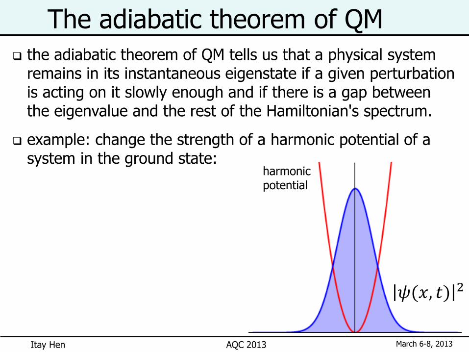
the adiabatic theorem of QM tells us that a physical system remains in its instantaneous eigenstate if a given perturbation is acting on it slowly enough and if there is a gap between the eigenvalue and the rest of the Hamiltonian's spectrum.
example: change the strength of a harmonic potential of a system in the ground state:
The adiabatic theorem of QM
𝜓(𝑥, 𝑡) 2
harmonic potential

Itay Hen March 6-8, 2013 AQC 2013
the adiabatic theorem of QM tells us that a physical system remains in its instantaneous eigenstate if a given perturbation is acting on it slowly enough and if there is a gap between the eigenvalue and the rest of the Hamiltonian's spectrum.
example: change the strength of a harmonic potential of a system in the ground state:
an abrupt change (a diabatic process):
The adiabatic theorem of QM
𝜓(𝑥, 𝑡) 2
harmonic potential

Itay Hen March 6-8, 2013 AQC 2013
the adiabatic theorem of QM tells us that a physical system remains in its instantaneous eigenstate if a given perturbation is acting on it slowly enough and if there is a gap between the eigenvalue and the rest of the Hamiltonian's spectrum.
example: change the strength of a harmonic potential of a system in the ground state:
a gradual slow change (an adiabatic process): wave function can “keep up” with the change.
The adiabatic theorem of QM
harmonic potential
𝜓(𝑥, 𝑡) 2
Itay Hen March 6-8, 2013 AQC 2013
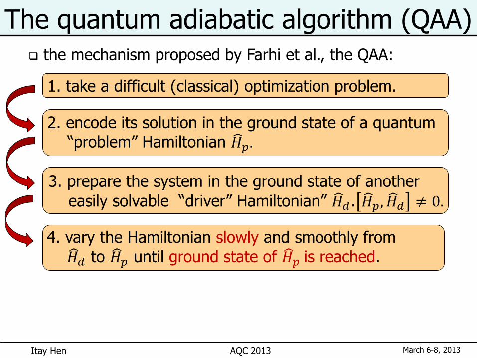
The quantum adiabatic algorithm (QAA)
1. take a difficult (classical) optimization problem.
4. vary the Hamiltonian slowly and smoothly from
𝐻 𝑑 to 𝐻 𝑝 until ground state of 𝐻 𝑝 is reached.
the mechanism proposed by Farhi et al., the QAA:
2. encode its solution in the ground state of a quantum
“problem” Hamiltonian 𝐻 𝑝.
3. prepare the system in the ground state of another
easily solvable “driver” Hamiltonian” 𝐻 𝑑. 𝐻 𝑝, 𝐻 𝑑 ≠ 0.
Itay Hen March 6-8, 2013 AQC 2013
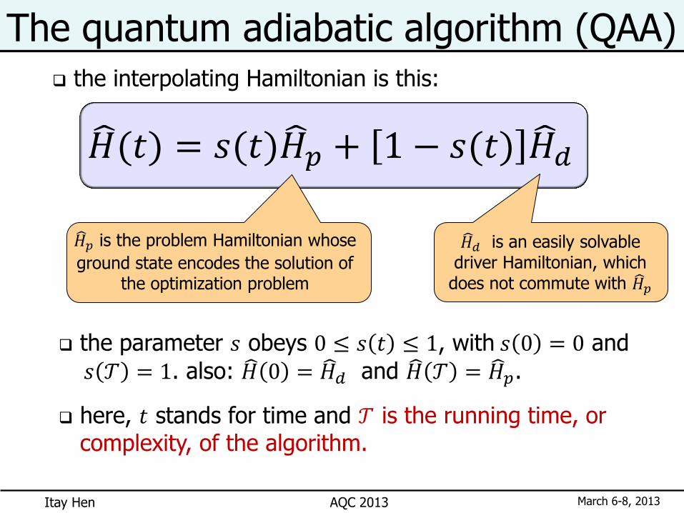
𝐻 (𝑡) = 𝑠(𝑡)𝐻 𝑝 + 1 − 𝑠(𝑡) 𝐻 𝑑
𝐻 𝑝 is the problem Hamiltonian whose
ground state encodes the solution of the optimization problem
𝐻 𝑑 is an easily solvable driver Hamiltonian, which
does not commute with 𝐻 𝑝
the interpolating Hamiltonian is this:
The quantum adiabatic algorithm (QAA)
the parameter 𝑠 obeys 0 ≤ 𝑠 𝑡 ≤ 1, with 𝑠 0 = 0 and 𝑠 𝒯 = 1. also: 𝐻 0 = 𝐻 𝑑 and 𝐻 𝒯 = 𝐻 𝑝.
here, 𝑡 stands for time and 𝒯 is the running time, or complexity, of the algorithm.
Itay Hen March 6-8, 2013 AQC 2013
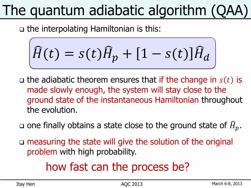
the adiabatic theorem ensures that if the change in 𝑠 𝑡 is
made slowly enough, the system will stay close to the ground state of the instantaneous Hamiltonian throughout the evolution.
one finally obtains a state close to the ground state of 𝐻 𝑝.
measuring the state will give the solution of the original problem with high probability.
the interpolating Hamiltonian is this:
The quantum adiabatic algorithm (QAA)
how fast can the process be?
𝐻 (𝑡) = 𝑠(𝑡)𝐻 𝑝 + 1 − 𝑠(𝑡) 𝐻 𝑑
Itay Hen March 6-8, 2013 AQC 2013
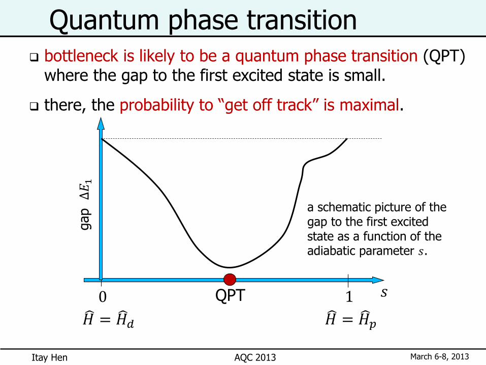
Quantum phase transition bottleneck is likely to be a quantum phase transition (QPT) where the gap to the first excited state is small.
there, the probability to “get off track” is maximal.
0 𝑠 1 QPT
𝐻 = 𝐻 𝑑 𝐻 = 𝐻 𝑝
gap
∆𝐸
1
a schematic picture of the gap to the first excited state as a function of the adiabatic parameter 𝑠.
Itay Hen March 6-8, 2013 AQC 2013
Quantum phase transition
𝒯 ∝ 1Δ𝐸𝑚𝑖𝑛
2
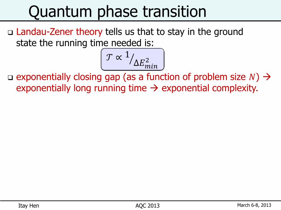
Landau-Zener theory tells us that to stay in the ground state the running time needed is:
exponentially closing gap (as a function of problem size 𝑁) exponentially long running time exponential complexity.

Itay Hen March 6-8, 2013 AQC 2013
Quantum phase transition
𝒯 ∝ 1Δ𝐸𝑚𝑖𝑛
2
Landau-Zener theory tells us that to stay in the ground state the running time needed is:
exponentially closing gap (as a function of problem size 𝑁) exponentially long running time exponential complexity.
it would be interesting to explore what one can do with “Local Adiabatic Evolution”, i.e., by slowing down when approaching the minimum gap etc. for example, the adiabatic algorithm for Grover’s search problem.
Itay Hen March 6-8, 2013 AQC 2013
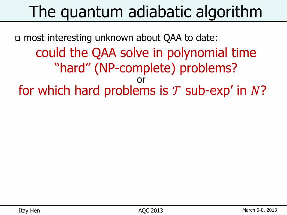
most interesting unknown about QAA to date:
The quantum adiabatic algorithm
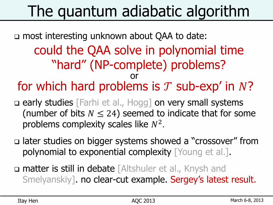
could the QAA solve in polynomial time “hard” (NP-complete) problems?
for which hard problems is 𝒯 sub-exp’ in 𝑁? or
Itay Hen March 6-8, 2013 AQC 2013
most interesting unknown about QAA to date:
early studies [Farhi et al., Hogg] on very small systems (number of bits 𝑁 ≤ 24) seemed to indicate that for some problems complexity scales like 𝑁2.
later studies on bigger systems showed a “crossover” from polynomial to exponential complexity [Young et al.].
matter is still in debate [Altshuler et al., Knysh and Smelyanskiy]. no clear-cut example. Sergey’s latest result.
The quantum adiabatic algorithm
could the QAA solve in polynomial time “hard” (NP-complete) problems?
for which hard problems is 𝒯 sub-exp’ in 𝑁? or
Itay Hen March 6-8, 2013 AQC 2013
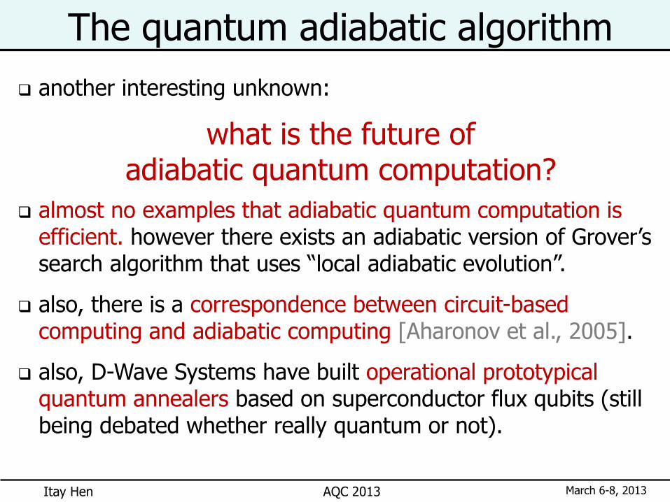
another interesting unknown:
almost no examples that adiabatic quantum computation is efficient. however there exists an adiabatic version of Grover’s search algorithm that uses “local adiabatic evolution”.
also, there is a correspondence between circuit-based computing and adiabatic computing [Aharonov et al., 2005].
also, D-Wave Systems have built operational prototypical quantum annealers based on superconductor flux qubits (still being debated whether really quantum or not).
The quantum adiabatic algorithm
what is the future of adiabatic quantum computation?
Itay Hen March 6-8, 2013 AQC 2013
Satisfiability problems

Itay Hen March 6-8, 2013 AQC 2013
Satisfiability problems here, we consider certain “constraint satisfaction” (SAT) problems that are known to be hard classically.
in SAT problems we ask whether there is an assignment of 𝑁 bits (or Ising spins) which satisfies all of 𝑀 clauses (or
logical conditions). bits in each clause are chosen at random.
Itay Hen March 6-8, 2013 AQC 2013
Satisfiability problems
𝑁 bits
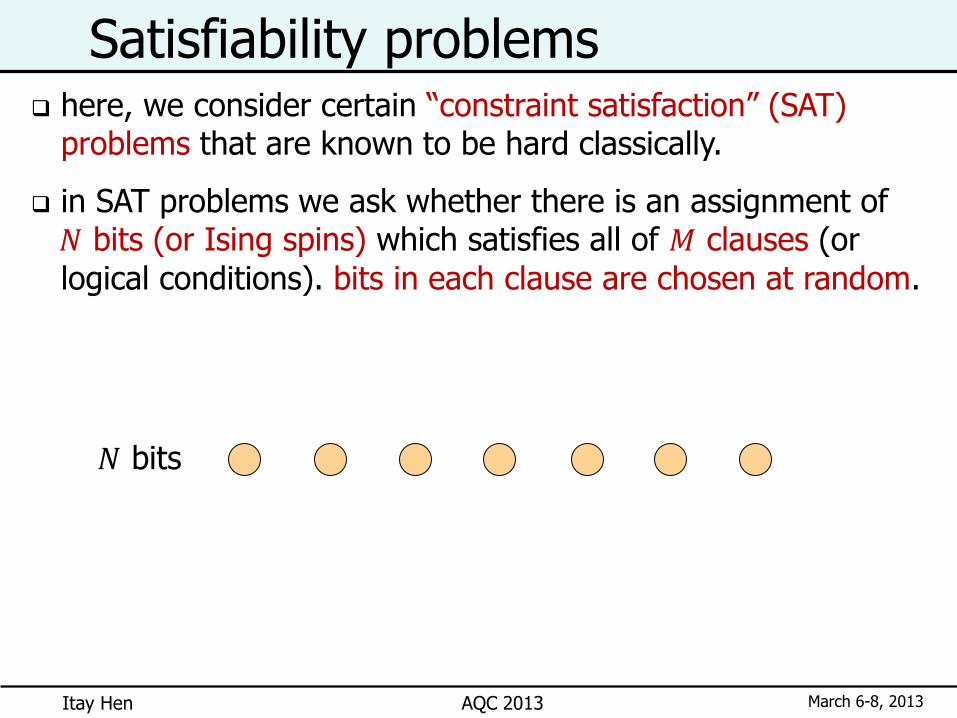
here, we consider certain “constraint satisfaction” (SAT) problems that are known to be hard classically.
in SAT problems we ask whether there is an assignment of 𝑁 bits (or Ising spins) which satisfies all of 𝑀 clauses (or
logical conditions). bits in each clause are chosen at random.
Itay Hen March 6-8, 2013 AQC 2013
Satisfiability problems
𝑁 bits
𝑀 clauses factor graph
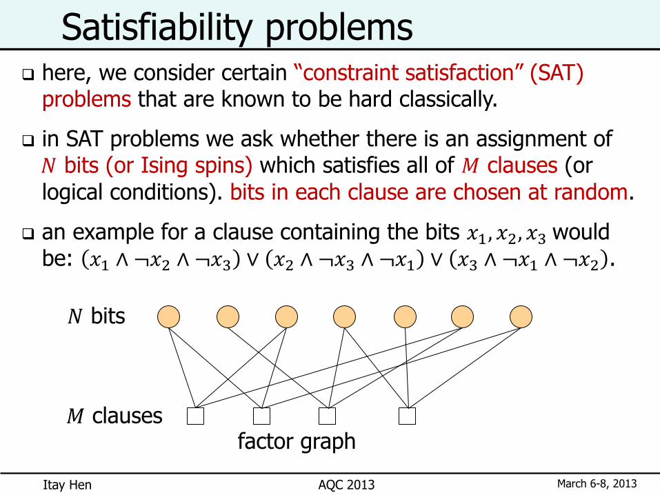
here, we consider certain “constraint satisfaction” (SAT) problems that are known to be hard classically.
in SAT problems we ask whether there is an assignment of 𝑁 bits (or Ising spins) which satisfies all of 𝑀 clauses (or
logical conditions). bits in each clause are chosen at random.
an example for a clause containing the bits 𝑥1, 𝑥2, 𝑥3 would be: 𝑥1 ∧ ¬𝑥2 ∧ ¬𝑥3 ∨ 𝑥2 ∧ ¬𝑥3 ∧ ¬𝑥1 ∨ 𝑥3 ∧ ¬𝑥1 ∧ ¬𝑥2 .
Itay Hen March 6-8, 2013 AQC 2013
Satisfiability problems
𝑁 bits
𝑀 clauses
0 1 0 1 1 0 0
√ √ √ √
factor graph
= a “satisfying assignment”
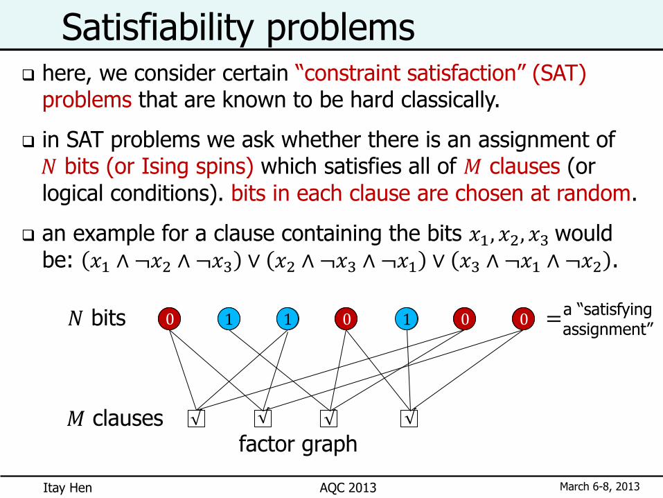
here, we consider certain “constraint satisfaction” (SAT) problems that are known to be hard classically.
in SAT problems we ask whether there is an assignment of 𝑁 bits (or Ising spins) which satisfies all of 𝑀 clauses (or
logical conditions). bits in each clause are chosen at random.
an example for a clause containing the bits 𝑥1, 𝑥2, 𝑥3 would be: 𝑥1 ∧ ¬𝑥2 ∧ ¬𝑥3 ∨ 𝑥2 ∧ ¬𝑥3 ∧ ¬𝑥1 ∨ 𝑥3 ∧ ¬𝑥1 ∧ ¬𝑥2 .

Itay Hen March 6-8, 2013 AQC 2013
Satisfiability problems for small 𝑀 𝑁 : easy to satisfy all clauses. exponential
number of solutions or “satisfying assignments” (SAT phase).
for large 𝑀 𝑁 : no satisfying solution exists (UNSAT phase).
we take the ratio of 𝑀 𝑁 to be at the satisfiability threshold,
where it is difficult to find a solution.
we study random instances with a unique satisfying assignment (USA). numerically more convenient because model is gapped.
𝑁 bits
𝑀 clauses
0 1 0 1 1 0 0
√ √ √ √
factor graph
= a “satisfying assignment”

Itay Hen March 6-8, 2013 AQC 2013
Satisfiability problems
the SAT problems we examined:
locked 1-in-3: a clause is a triplet of bits picked at random from a pool of 𝑁 bits. it is satisfied if and only if
exactly one bit is 1 and the other two are 0.
locked 2-in-4: same as above only with 2 bits out of 4 in each clause that must be 1 [Zdeborová & Mézard, 08].
3-regular 3-xorsat [Jörg et al]: here, each bit is exactly in 3 clauses and a clause is satisfied if the sum of the 3 bits in a clause (mod 2) is a value specified (0 or 1). this problem is in P. factor graph
of 3-regular 3-xorsat
Itay Hen March 6-8, 2013 AQC 2013
The encoding Hamiltonians
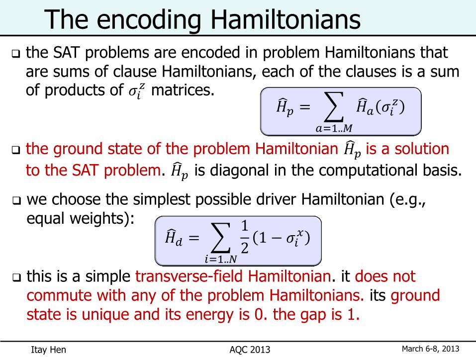
we choose the simplest possible driver Hamiltonian (e.g., equal weights):
this is a simple transverse-field Hamiltonian. it does not commute with any of the problem Hamiltonians. its ground state is unique and its energy is 0. the gap is 1.
𝐻 𝑑 = 1
21 − 𝜎𝑖
𝑥
𝑖=1..𝑁
the SAT problems are encoded in problem Hamiltonians that are sums of clause Hamiltonians, each of the clauses is a sum of products of 𝜎𝑖
𝑧 matrices.
the ground state of the problem Hamiltonian 𝐻 𝑝 is a solution
to the SAT problem. 𝐻 𝑝 is diagonal in the computational basis.
𝐻 𝑝 = 𝐻 𝑎 𝜎𝑖𝑧
𝑎=1..𝑀
Itay Hen March 6-8, 2013 AQC 2013
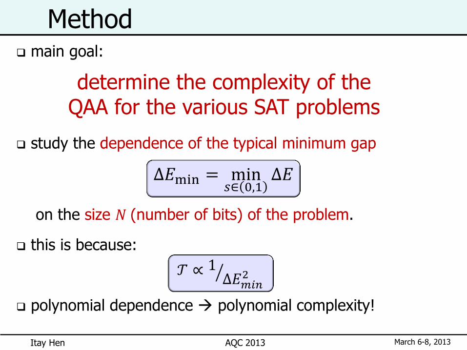
main goal:
study the dependence of the typical minimum gap
on the size 𝑁 (number of bits) of the problem.
this is because:
polynomial dependence polynomial complexity!
Method
determine the complexity of the QAA for the various SAT problems
𝒯 ∝ 1Δ𝐸𝑚𝑖𝑛
2
Δ𝐸min = min𝑠∈ 0,1
Δ𝐸
Itay Hen March 6-8, 2013 AQC 2013
Method
for each given problem we study several system sizes,
because we are interested in size-dependence.
we consider typically 50 instances per problem size.
to obtain “typical behavior” we take medians.
for each instance, we measure the gap of the system for
several values of the parameter 𝑠 in order to obtain an
accurate estimation of the minimum gap.
for each 𝑠 value, we run a quantum Monte Carlo (QMC)
simulation to obtain the gap numerically (and other
measureable quantities).
Itay Hen March 6-8, 2013 AQC 2013
for large system sizes, we can not use exact diagonalization.
we employ a continuous-time quantum Monte Carlo (QMC)
technique.
an additional periodic dimension of imaginary time 0 ≤ 𝜏 < 𝛽.
𝛽 is the inverse-temperature obeying 𝛽∆𝐸1 ≫ 1.
with QMC we do a sampling of the 2𝑁 states of the Hilbert
space. exact-numerical up to statistical errors.
QMC enables access to the equilibrium properties of the
system but also provides indirect access to the system gap.
here, we basically simulate spin-1 2 systems with different
interactions and different sizes.
we employ parallel tempering (swapping configurations of
adjacent 𝑠 values) which speeds up equilibration.
Quantum Monte Carlo
Itay Hen March 6-8, 2013 AQC 2013
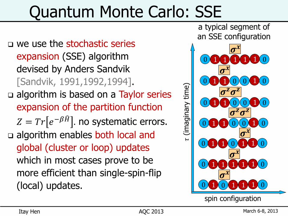
we use the stochastic series
expansion (SSE) algorithm
devised by Anders Sandvik
[Sandvik, 1991,1992,1994].
algorithm is based on a Taylor series
expansion of the partition function
𝑍 = 𝑇𝑟 𝑒−𝛽𝐻 . no systematic errors.
algorithm enables both local and
global (cluster or loop) updates
which in most cases prove to be
more efficient than single-spin-flip
(local) updates.
Quantum Monte Carlo: SSE a typical segment of an SSE configuration
1 0 1 0 0 1 1
𝝈𝒙
𝝈𝒙
𝝈𝒙
𝝈𝒙
𝝈𝒙
1 0 1 0 0 1 1
𝝈𝒛𝝈𝒛
𝝈𝒛𝝈𝒛
spin configuration
𝜏 (im
agin
ary
tim
e)
1 0 1 0 1 1 1
1 0 1 0 0 1 0
1 0 1 0 0 1 0
1 0 1 0 0 1 0
1 0 1 0 1 1 1

Itay Hen March 6-8, 2013 AQC 2013
we extract the gap of the system by measuring and analyzing different-imaginary-time correlation functions of certain operators:
if 𝛽Δ𝐸1 ≫ 1 (system is in its ground state) then at long
imaginary times we have:
i.e., only the slowest-decaying exponent survives (provided that the corresponding matrix element does not vanish).
Extracting the gap
𝐶𝐴 𝜏 = 𝐴 𝜏 𝐴 0 − 𝐴 2
𝐶𝐴 𝜏 ≅ 0|𝐴 |12𝑒−Δ𝐸1𝜏
Itay Hen March 6-8, 2013 AQC 2013
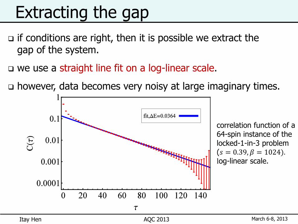
if conditions are right, then it is possible we extract the gap of the system.
we use a straight line fit on a log-linear scale.
however, data becomes very noisy at large imaginary times.
Extracting the gap
correlation function of a 64-spin instance of the locked-1-in-3 problem (𝑠 = 0.39, 𝛽 = 1024). log-linear scale.

Itay Hen March 6-8, 2013 AQC 2013
QMC results
main goal: to determine the complexity of the QAA for the
various SAT problems.
for each of the problems studied, we look at the dependence
of the typical (median) minimum gap on the size of the
problem.
a polynomially decreasing gap would mean a polynomially
increasing running time and hence QAA could be called
efficient.
an exponentially decreasing gap would mean that the QAA is
not more efficient than the best classical algorithm.
heavy QMC simulations. hundreds/thousands of cores,
running in some cases for weeks/months.
Itay Hen March 6-8, 2013 AQC 2013
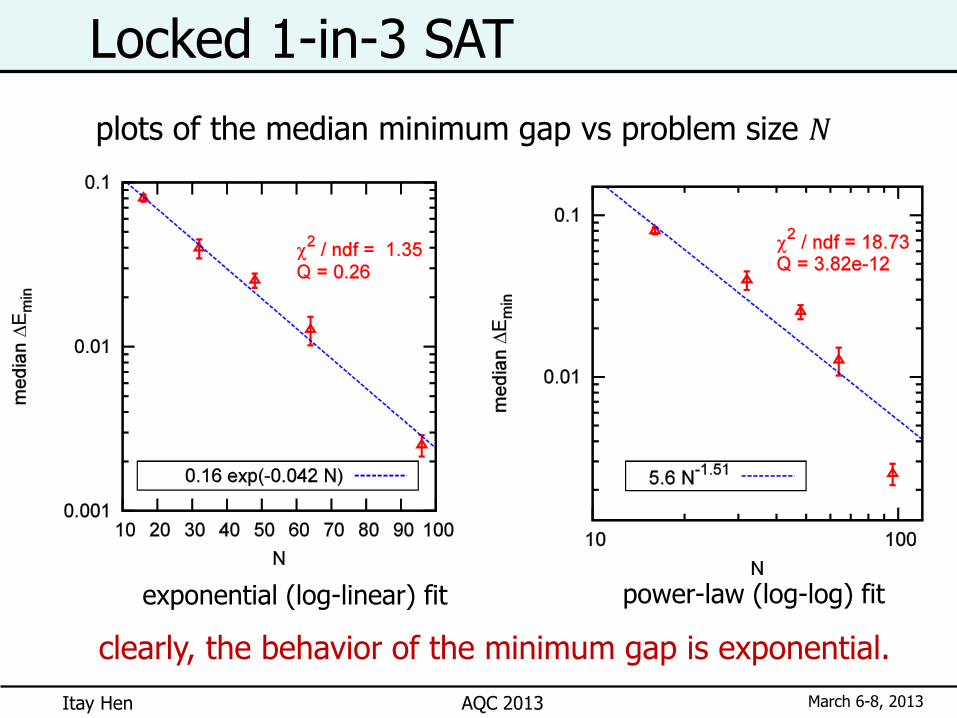
Locked 1-in-3 SAT
plots of the median minimum gap vs problem size 𝑁
exponential (log-linear) fit power-law (log-log) fit
clearly, the behavior of the minimum gap is exponential.
Itay Hen March 6-8, 2013 AQC 2013
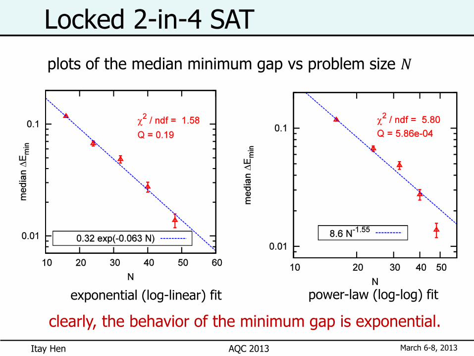
Locked 2-in-4 SAT
plots of the median minimum gap vs problem size 𝑁
exponential (log-linear) fit power-law (log-log) fit
clearly, the behavior of the minimum gap is exponential.
Itay Hen March 6-8, 2013 AQC 2013
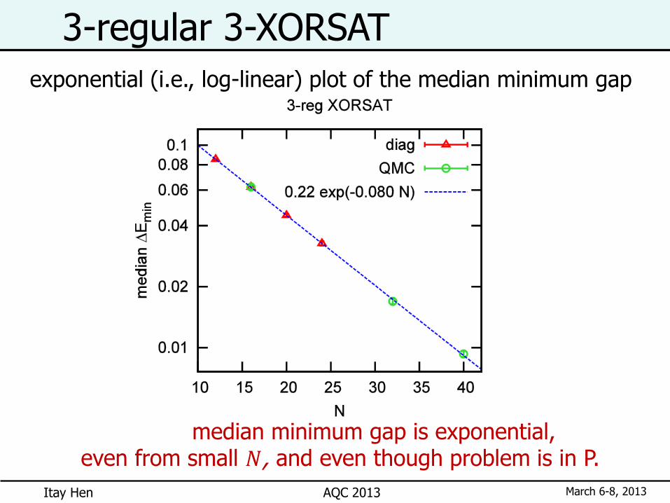
3-regular 3-XORSAT
exponential (i.e., log-linear) plot of the median minimum gap
median minimum gap is exponential, even from small 𝑁, and even though problem is in P.

Itay Hen March 6-8, 2013 AQC 2013
WalkSAT is a classical, heuristic, local search algorithm.
it is a reasonable classical algorithm to compare with QAA [Guidetti and Young, 2010].
the algorithm itself is very simple:
pick at random an unsatisfied clause and flip a bit in that clause.
with some probability this bit is chosen to be the one which causes the fewest previously satisfied clauses to become unsatisfied, and otherwise it is chosen at random.
repeat until the number of unsatisfied clauses is zero.
Comparison with a classical algorithm

Itay Hen March 6-8, 2013 AQC 2013
Comparison with a classical algorithm WalkSAT is a classical, heuristic, local search algorithm.
it is a reasonable classical algorithm to compare with QAA [Guidetti and Young, 2010].
the complexity of WalkSAT is determined by the amount of “bit flips” the algorithm performs until it reaches a solution.
for the QAA, we have
we can therefore compare exponent coefficients.
𝒯 ∝ 𝑁flips~ exp [𝜇𝑁]
𝒯 ∝ exp [2𝑐𝑁] for Δ𝐸1 ∝ exp [−𝑐𝑁]

Itay Hen March 6-8, 2013 AQC 2013
running times are proportional to exp [𝜇𝑁] where 𝑁 is system size.
WalkSAT is better, however we see the same trend.
important to remember: we used here the simplest implementation of the QAA for instances with USA. algorithm can certainly be improved.
a comparison of the 𝜇 values among the different models and between QAA and WalkSAT
Comparison with a classical algorithm

Itay Hen March 6-8, 2013 AQC 2013
3-regular random antiferromagnet
(3-reg Max-Cut)
Itay Hen March 6-8, 2013 AQC 2013
3-regular Max-Cut
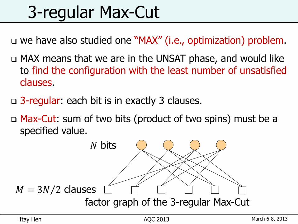
we have also studied one “MAX” (i.e., optimization) problem.
MAX means that we are in the UNSAT phase, and would like to find the configuration with the least number of unsatisfied clauses.
3-regular: each bit is in exactly 3 clauses.
Max-Cut: sum of two bits (product of two spins) must be a specified value.
𝑁 bits
𝑀 = 3𝑁 2 clauses
factor graph of the 3-regular Max-Cut
Itay Hen March 6-8, 2013 AQC 2013
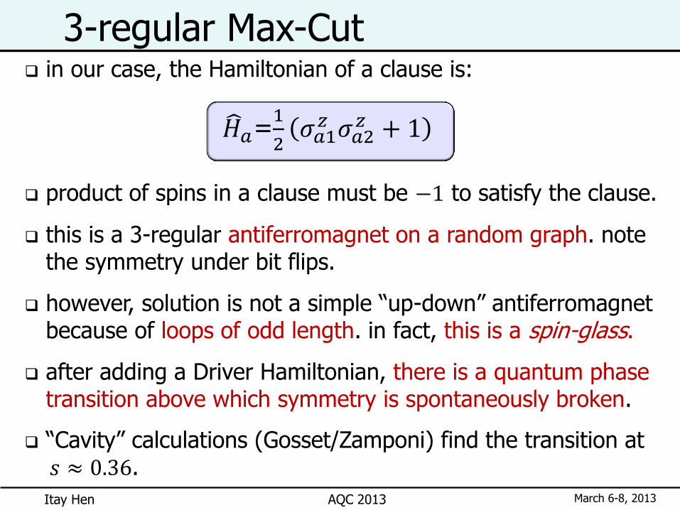
3-regular Max-Cut in our case, the Hamiltonian of a clause is:
product of spins in a clause must be −1 to satisfy the clause.
this is a 3-regular antiferromagnet on a random graph. note the symmetry under bit flips.
however, solution is not a simple “up-down” antiferromagnet because of loops of odd length. in fact, this is a spin-glass.
after adding a Driver Hamiltonian, there is a quantum phase transition above which symmetry is spontaneously broken.
“Cavity” calculations (Gosset/Zamponi) find the transition at 𝑠 ≈ 0.36.
𝐻 𝑎=1
2𝜎𝑎1
𝑧 𝜎𝑎2𝑧 + 1
Itay Hen March 6-8, 2013 AQC 2013
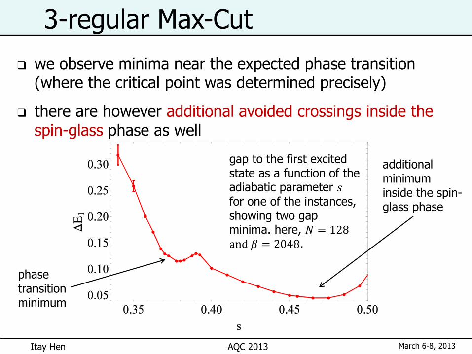
3-regular Max-Cut
we observe minima near the expected phase transition (where the critical point was determined precisely)
there are however additional avoided crossings inside the spin-glass phase as well
gap to the first excited state as a function of the adiabatic parameter 𝑠 for one of the instances, showing two gap minima. here, 𝑁 = 128 and 𝛽 = 2048.
phase transition minimum
additional minimum inside the spin-glass phase
Itay Hen March 6-8, 2013 AQC 2013
3-regular Max-Cut
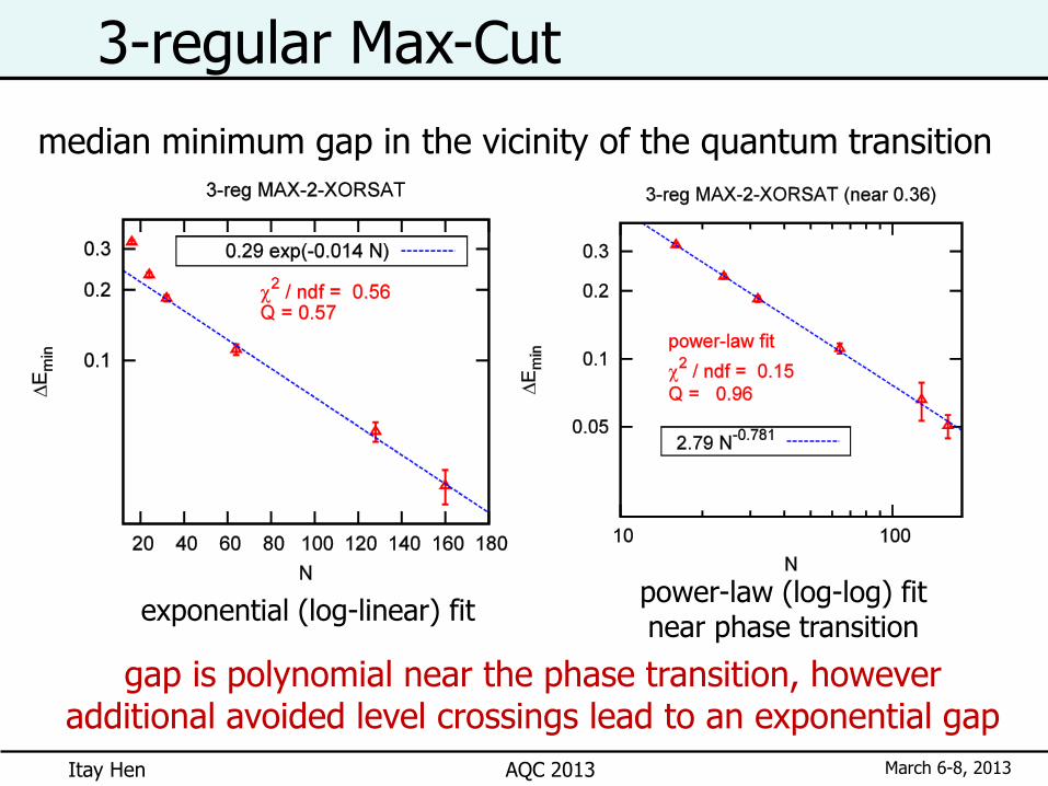
median minimum gap in the vicinity of the quantum transition
exponential (log-linear) fit power-law (log-log) fit near phase transition
gap is polynomial near the phase transition, however additional avoided level crossings lead to an exponential gap
Itay Hen March 6-8, 2013 AQC 2013
The graph isomorphism problem
Itay Hen March 6-8, 2013 AQC 2013
The graph isomorphism problem
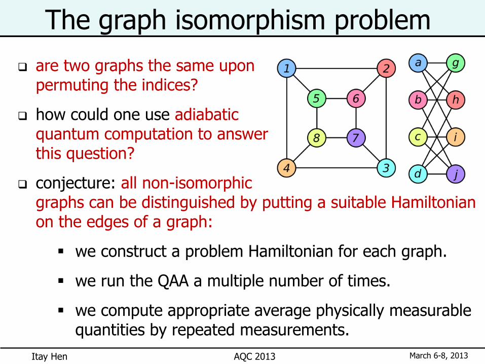
are two graphs the same upon permuting the indices?
how could one use adiabatic quantum computation to answer this question?
conjecture: all non-isomorphic graphs can be distinguished by putting a suitable Hamiltonian on the edges of a graph:
we construct a problem Hamiltonian for each graph.
we run the QAA a multiple number of times.
we compute appropriate average physically measurable quantities by repeated measurements.
Itay Hen March 6-8, 2013 AQC 2013
The graph isomorphism problem
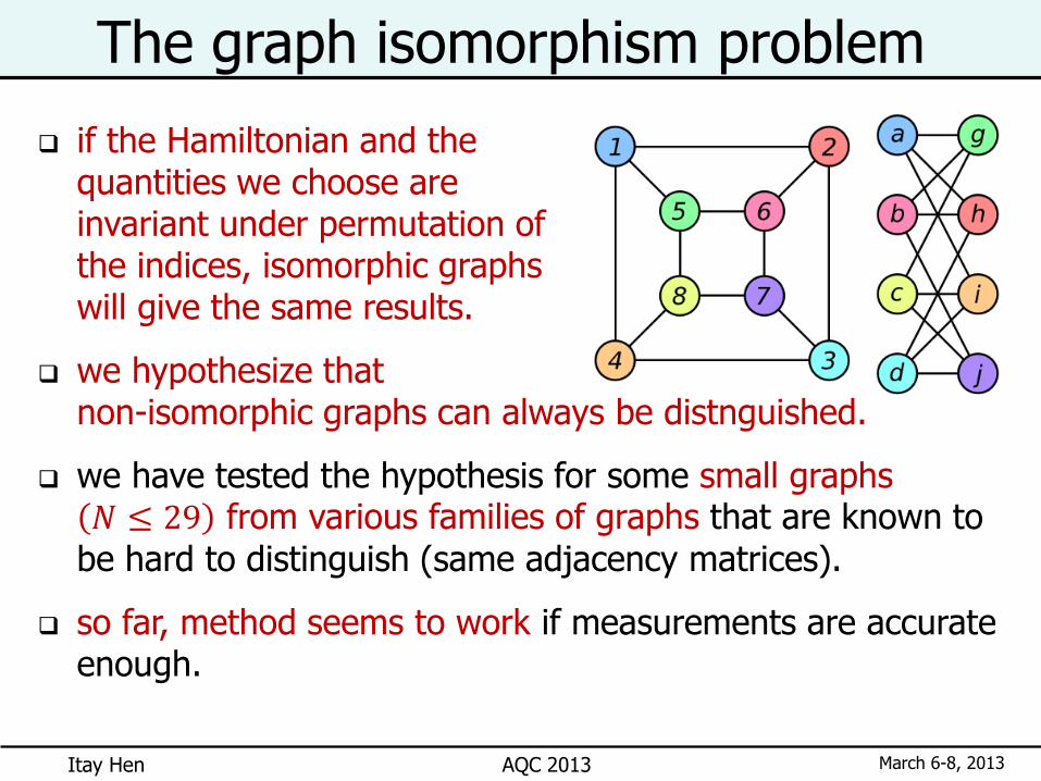
if the Hamiltonian and the quantities we choose are invariant under permutation of the indices, isomorphic graphs will give the same results.
we hypothesize that non-isomorphic graphs can always be distnguished.
we have tested the hypothesis for some small graphs 𝑁 ≤ 29 from various families of graphs that are known to
be hard to distinguish (same adjacency matrices).
so far, method seems to work if measurements are accurate enough.
Itay Hen March 6-8, 2013 AQC 2013
The graph isomorphism problem
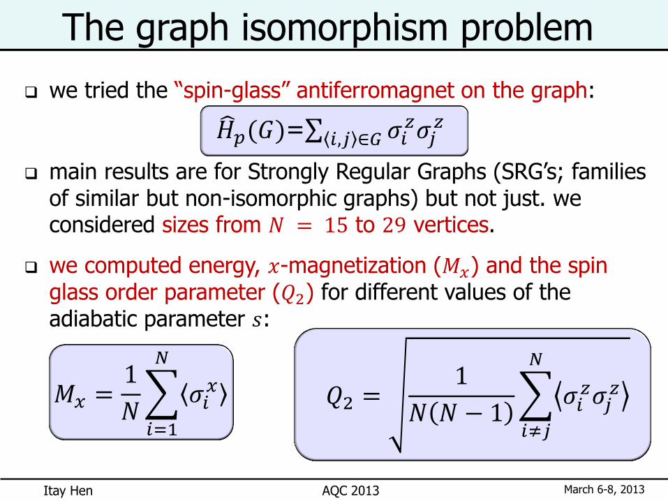
we tried the “spin-glass” antiferromagnet on the graph:
main results are for Strongly Regular Graphs (SRG’s; families of similar but non-isomorphic graphs) but not just. we considered sizes from 𝑁 = 15 to 29 vertices.
we computed energy, 𝑥-magnetization (𝑀𝑥) and the spin glass order parameter (𝑄2) for different values of the adiabatic parameter 𝑠:
𝐻 𝑝(𝐺)= 𝜎𝑖𝑧𝜎𝑗
𝑧𝑖,𝑗 ∈𝐺
𝑀𝑥 =1
𝑁 𝜎𝑖
𝑥
𝑁
𝑖=1
𝑄2 =1
𝑁 𝑁 − 1 𝜎𝑖
𝑧𝜎𝑗𝑧
𝑁
𝑖≠𝑗
Itay Hen March 6-8, 2013 AQC 2013
The graph isomorphism problem
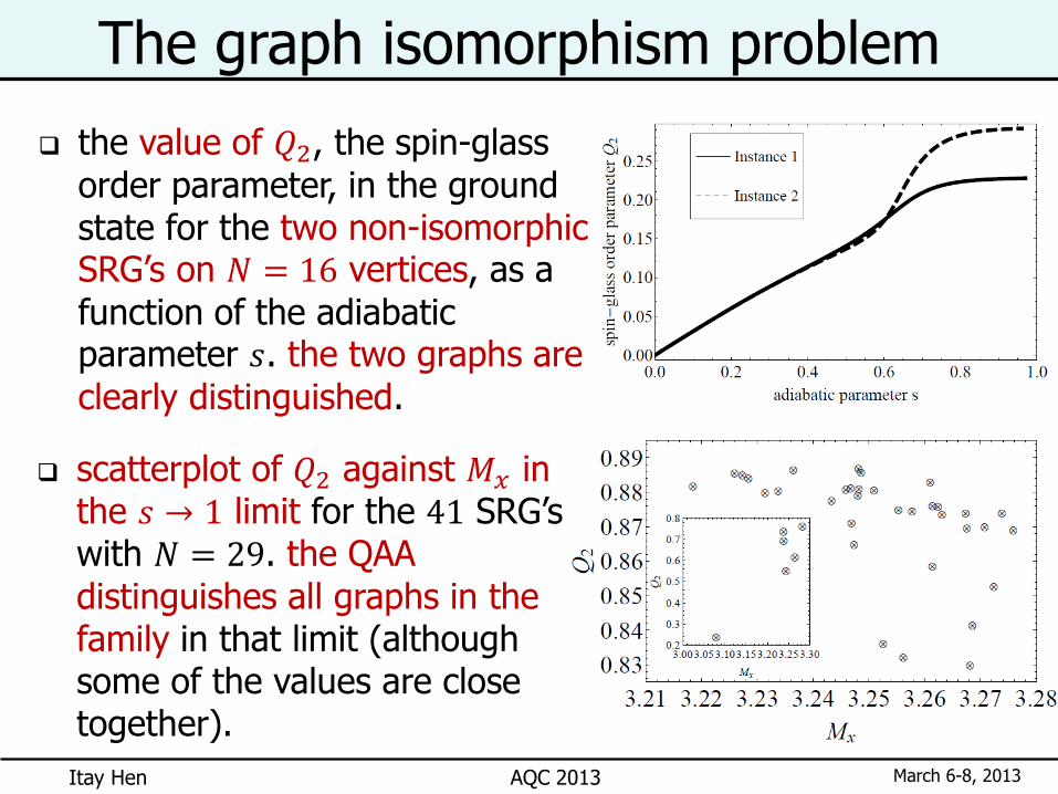
the value of 𝑄2, the spin-glass order parameter, in the ground state for the two non-isomorphic SRG’s on 𝑁 = 16 vertices, as a
function of the adiabatic parameter 𝑠. the two graphs are
clearly distinguished.
scatterplot of 𝑄2 against 𝑀𝑥 in the 𝑠 → 1 limit for the 41 SRG’s with 𝑁 = 29. the QAA
distinguishes all graphs in the family in that limit (although some of the values are close together).
Itay Hen March 6-8, 2013 AQC 2013
The graph isomorphism problem perhaps there are “better” Hamiltonians than the one chosen
here. here, we have used “glassiness” to solve the graph isomorphism problem.
perhaps there are better measurements that can be performed in order to distinguish between graphs, e.g., susceptibilities. here, we have mainly used the spin-glass order parameter.
can be tested experimentally on existing D-Wave hardware with relatively minor modifications.
it is unclear whether or not the algorithm is efficient. what is the nature of the quantum phase transition? need to investigate size-dependence of minimum gap.
clearly more testing is needed.
Itay Hen March 6-8, 2013 AQC 2013
Conclusions and future research
Itay Hen March 6-8, 2013 AQC 2013
for the SAT problems investigated, we don’t find that QAA is better
than state-of-the-art classical algorithms.
we find that the harder a problem is for classical algorithms
(WalkSAT), the harder it is also for the QAA.
for the Max-Cut (random antiferromagnet) problem, results point to
a polynomially decreasing gap near the quantum phase transition.
it seems however that the overall gap behavior is exponential.
QAA seems to be able to solve the graph isomorphism problem
(more tests are needed) however the efficiency of the algorithm is
not yet known.
Conclusions