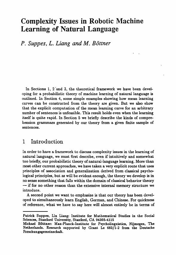
Complexity Issues in Robotic Machine Learning of Natural Language

P. Suppes, L. Liang and M. Böttner

In Sections 1, 2 ‘and 3, the theoretical framework we have been devel- oping for a probabilistic theory of machine learning of natural language is outlined. In Section 4, some simple examples showing how mean learning curves can be constructed from the theory are given. But we also show that the explicit computation of the mean learning curve for an arbitrary number of sentences is unfeasible. This result holds even when the learning itself is quite rapid. In Section 5 we briefly describe the kinds of compre- hension grammars generated by our theory from a given finite sample of sentences.

l Introduction

In order to have a framework to discuss complexity issues in the learning of natural language, we must first describe, even if intuitively and somewhat too briefly, our probabilistic theory of natural-language learning. More than most other current approaches, we have taken a very explicit route that uses principles of association and generalization derived from classical psycho- logical principles, but as will be evident enough, the theory we develop is in no sense something that falls within the domain of classical behavior theory - if for no other reason than the extensive internal memory structure we introduce.

A second point we want to emphasize is that our theory has been devel- oped to simultaneously learn English, German, and Chinese. For quickness of reference, what we have to say here will almost entirely be in terms of

Patrick Suppes, Lin Liang: Institute for Mathematica3 Studies in the Social Sciences, Stanford University, Stanford, CA 94305-4115 Michael Bõttner: Max-Planck-Institute for Psycholinguistics, Nijmegen, The Netherlands. Research supported by Grant Le 683/1-2 from the Deutsche Forschungsgemeinschaft.

Before formulating the learning principles we use, we nee mally certain assumptions about the cognitive and perceptual capacities of the class of robots we work with.

Internal I;anguage. We assume the robot has a fully developed internal language which it does not learn. It is technically important, but not con- ceptually fundamental that in the present case this language is LISP. (FOP more details, see Section 3.) What must be emphasized is that when we speak here of the internal language we refer only to the language of the internal representation, which is itself a language of a higher level of ab- straction, relative to the concrete movements and perceptions of the robot. There are severd other internal language modules that were either devel- oped by us or that come in the software package with Robotworld. It has been important to us that most of the machine learning of a given natural language can take glace through simulation of the robot’s behavior just at the level of the language of the internal representation.

Objects, Relations an¿ Properties. We furthermore assume the robot begins its natural language learning with all the basic cognitive and per- ceptual concepts it will have. This means that our first language learning experiments are pure language learning. For example, we have assumed that the spatial relations frequently referred to in all the languages we COR-

104

sider in detail are already known to the robot. This is of course contrary to human language learning. There is good evidence, for example, that most children do not understand the relations of left and right, even at the age of thirty-six months when their command of language is already extremely good.

Actions. What was just said about objects and relations applies also to actions. There are in the internal language symbols for a fixed set of possible actions. The problem is only to learn their particular linguistic representation in a given language. What has been said about objects, relations, properties and actions constitutes a permanent part of memory of the robot. This memory does not change and is therefore not involved in the learning theory we formulate. (It is obvious that in a more general theory we will want to include learning of new concepts, etc.)

1.2 INTUITIVE DESCRIPTION OF T H E PROCESS OF LEARNING

What we want to describe now is the process of learning in terms of the various events that happen on a given trial. First, the robot begins a trial in a given state of memory. There are three parts of this memory that are changed due to learning. The first is the association relation between words of a given language and internal symbols that represent denotations of members of categories in the internal representation language. For exam- ple, the action of putting will be represented internally, let us say, by the symbol $ p and will have three different linguistic representations in English, German and Chinese. The problem will be to learn in each language what word is properly associated with the internal representation $p. The same process of association must be learned for objects, properties and spatial relations. But knowing such associations is not enough, contrary to some naive theories of associationism.

It is also important to have grammatical forms. We will not try to lay out everything about grammatical forms that we have in our fully stated theory, but it will be useful to give some examples. Consider the verbal command Get the screw!This would be an instance of the grammatical form A the O!, where A is the category of actions and O is the category of objects. As might be expected we do not actually have just a single category of actions, but several subcategories, depending upon the number of arguments required, etc. The central point here, however, is the nature of a grammatical form. The grammatical forms are derived only from actual instances of verbal commands given to the robot. Secondly, associated with each grammatical form are the first associations of words with their internal interpretations. So for example, if Get the screw! had been the first occurrence on which the grammatical form just stated was generated, then also stored with that grammatical form would be the associations get - $g, screw - %-we use $9 for the internal symbol corresponding correctly to get , and sometimes

105

we just use g for get, as in the trees shown later. Similar conventions apply to other denoting words. The third part of memory that varies is the short- term memory that holds a given verbal command for the period of the trial on which it is effective. This memory content decays and is not available for access after the trial on which a particular command is given. So at the beginning of the trial this short term buffer is empty, but is filled by the second step in learning. A verbal command is given to the robot and it is held in memory in the short-term buffer.

The third step is for the learning program to look up the associations of the words in the verbal command that has been given. If associations exist for any of the words, the categories of the associations, which are the categories of the internal interpretation, are also retrieved. The categories are substituted for the associated words and an effort is then made to generate recursively the resulting grammatical form. For example, if mis- takenly the word get had been associated to $8, the internal symbol for screw, and scfew had been associated with $g, the internal symbol for get, then the grammatical form that would have been generated and now found upon a second occurrence of the verbal command would be O fhe A! Now if there were no such grammatical form generated, once the associations were formed such a grammatical form would be created by the process of generalization which is used to generate grammatical forms.

When a grammatical form is stored in memory, also associated with this grammatical form in memory is its internal representation. This is an important part of the memory that changes with learning as well. If the grammatical form is generated, the internal representation is then used to execute the verbal command that has been given. If the command is executed correctly then the robot is ready for a new learning trial.

The important case of learning is when no grammatical form can be generated recursively from the grammatical forms in memory to match the form of the given verbal command. In this case the robot is unable to make a response. The correct response must be coerced. On the basis of this coercion, a new internal representation is formed. At this point the critical step comes of a probabilistic association between words of the verbal utterance and the internal denoting symbols of the new internal representation. This probabilistic association is assumed to be on a uniform probability basis. For example, if within the new internal representation there are two internal denoting symbols and there are no words in the verbal command associated to either of these internal symbols, and there are four words in the verbal command, then any pair of the four will be as likely to be associated with the pair of internal symbols as any other pair. After this-association is made, a new grammatical form is generated, and possibly because of the new associations at least one of the old grammatical forms is deleted, for one of the axioms states that a word or internal denoting symbol can have exactly one association, so when a new association is formed for a word any old associations must be deleted. (This strong all-or-none

ar we are cone

faci~itate the statement of rinciples governing escribed, certain notational conventio~s atin letters to refer to verbal ~ommands

ural language, and 'we use Greek letters to refer The letters a , ai S B etc. refer to words in a verb

ets. to internal denotations. to terms of a ve

forms - either sentential or ) to show a category argument

presentations of a gram~atical ur Greek-Latin letter conven-

tion in the case of semantic categories or category variables X, Xrp Y', etc. We use the same category symbols in both grammatical forms and their internal representations. We now turn to the statement of the axioms of learning in intuitive form. We will give a more formal and explicit state- ment in a longer version. We have delayed until Section 5 statement of the most technical axioms, the one on term association and the one on term form substitution, which are used to generate recursive grammatical forms.

2.1 AXIOMS OF LEARNING l. (Assoczation by contiguity). If verbal command s is contiguous with a

coerced action that has internal representation u, then s is associated with Q, i.e., in symbols s B.

2. (Probabilistic association). If s u, s has a set ( u i } of denoting words - not associated with any internal denotations of u, and u has a set

{q} of internal symbols not associated with any words of s, then an element of {ai 1 is uniformly sampled without replacement from {ui} I

at the same time an element of {ai} is correspondingly sampled, and

107

the sampled pair are associated, i.e., ai CY^. Sampling continues until there is no remaining ai or ai.

3. (Prior associations). When a word in a verbal command or an internal symbol is given a new association (Axiom 2), any prior associations of that word or symbol are deleted from memory.

4. (Forgetting associations of commands). An association s - u of a verbal command s is held only temporarily in memory until the action represented internally by o is executed or until all word associations are complete (Axiom 2).

5. (Correction procedure). If a verbal command s cannot be executed or is executed incorrectly with s - o, and if a correct response with internd representation u' is coerced, then s is associated with u' for application of Axiom 2.

6. (Category genenalization). If t - T and r E X then t E X .

7. (Gmmmat ica l f o n n genemliraiion). If g ( t ) - y(r), t - T and t E X. then g ( X ) - 7 ( X ) .

9. (Memory trace for a grammatical f o m ) . The first time a grammatical generdization ( X ) (Axiom 7) is formed, the word associations on which the generdization is based are stored with it.

10. (Elimination of a grammatical fo rm) . If a memory-trace association a - CY for g is eliminated (Axiom 3), then g is eliminated from mem- ory.

3 Internal Representation

In this section we sketch the language of internal representation we use. As already mentioned, for purposes of our robotic application we use LISP as the language of representation. Internal representations will therefore be LISP-expressions. A LISP-expression is any string (El ... E,,) where El, ...( L are either atoms or LISP-expressions.

The fragments of natural language are meant to instruct a robot to per- form elementary actions in a simple environment. Due to the capabili- ties of the robot the tasks are moving around in a 3D space and opening (and closing) the gripper. The environment is a collection of objects like screws, nuts, washers, plates, sleeves of a limited number of colors, sizes. and shapes. Commands that typically arise in this context are: Open the gripper! Move forward! lkrn t o the left! Put a nut on the screw! GO t o

to determine the object of

objects in the robot’s

then takes this set of all screws of the environment as input and returns a unique screw from this set. This particular screw together with the action $g is the input of the operation fa l .

According to the semantic category of the object that it denotes, eac expression of our language of internal representation belongs to a certain category. In the above example, e.g., the expression screw belongs to the category property, more specifically: object property, and the expression get belongs to the category action. The list of categories is as follows: Property (P), Spatial Relation, (R), Action ( A ) , and Object (O).

Semantic categories can be further divided into subcategories. The cat- egory R of spatial relations is split up into subcategories R1 and R2 de- pending on whether its elements are binary or ternary relations. Associated with the category R is the semantic operation form pmperty, abbreviated as fp, which takes a relation and object as input and returns a property - examples are to be found in Section 5. The category A of actions has six subcategories depending OB the valency of the action expression. So we have a subcategory for actions that do not require any complement like stop, another subcategory for actions that require an object like get, a sub- category for actions that require a region as complement like go as in, e.g. Go near a plate! a subcategory for actions that require both an object and

109

a region like put, as in e.g. Put a screw near a plafe! a subcategory for actions that require a direction as their complement like turn, as in e.g. Turn left!, a d a subcategory for actions that require both an object and a direction as in e.g. Move the screw forwad! Unlike the subcategories of relatiom the subcategories of actions are not disjoint, i.e. an action like, e.g. turn, occurs in more than one category.

4 Mean Learning Curves

Mean learning curves represent the average of all possible individual learn- ing curves. Such mean curves have several important features. First, by abstracting from the details of individual curves they give a sense of the rate of learning to be expected. In the case of machine learning this can be important in evaluating the practicality of the theory proposed. If the expected number of trials to reach a satisfactory learning criterion is 21000, for example, then the theory is not of practical interest. Second, mean learning curves typically exhibit a theoretical robustness that is not char- acteristic of individual learning curves, i.e., in probabilistic terms, individ- ual sample paths. Many minor theoretical details and, on occasion, major ones as well, can be modified without changing the theoretically predicted mean learning curve. A familiar example is the mean learning curve that is identical for one-parameter linear incremental models of simple learn- ing and one-parameter all-or-none Markov models of the same phenomena. The predicted individual sample paths are completely different for the two kinds of models, but the mean learning curves are identical.

4.1 SIMPLE EXAMPLES Because in simple cases we can theoretically compute the mean learning curve from the axioms of Section 2, we will first consider some very simple cases that give an insight into how things work. These cases are so simple that no actual simulation is needed. In the analyses we shall consider, let

m = number of distinct commands, d = number of distinct denoting words, k = average number of denoting words per command.

In the case of parameter k, in the simple cases we consider k is not simply an average but a constant.

Case 1. m = 3, d = 3, k = 1. An example of this case would be simply three commands: Fornard!, Left! and Right! Because we have three com- mands and three denoting words with one occurring in each sentence, it is quite easy to derive the mean probability of a correct response on trial n. It is apparent at once under the condition that we present a block of the three commands randomly sampling without replacement. Such a block is

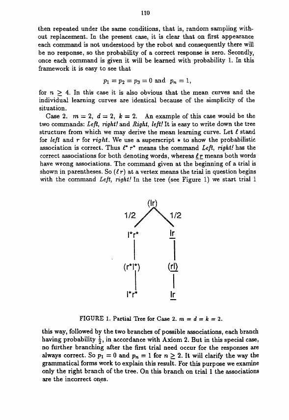
this way, followed by the two branches of possible associations, each branch having probability 4, in accordance with Axiom 2. But in this special case, no further branching after the first trial need occur for the responses are always correct. So p1 = O and p,, = 1 for n 2 2. It will clarify the way the grammatical forms work to explain this result. For this purpose we examine only the right branch of the tree. On this branch on trial 1 the associations are the incorrect onFs.

111

The grammatical form generated and its associated internal form are then:

A' A - I (A , A')

Note that on the left branch this reversal of order of A and A' between the grammatical form and the associated internal form does not take place:

A A' - I(A, A') (left branch)

But in this restricted, simpleminded but instructive, example, either gram- matical form works for its branch.

The next two cases are perhaps the simplest which have a nontrivial mean learning curve, i.e., the curve is not just a (OJ) step function.

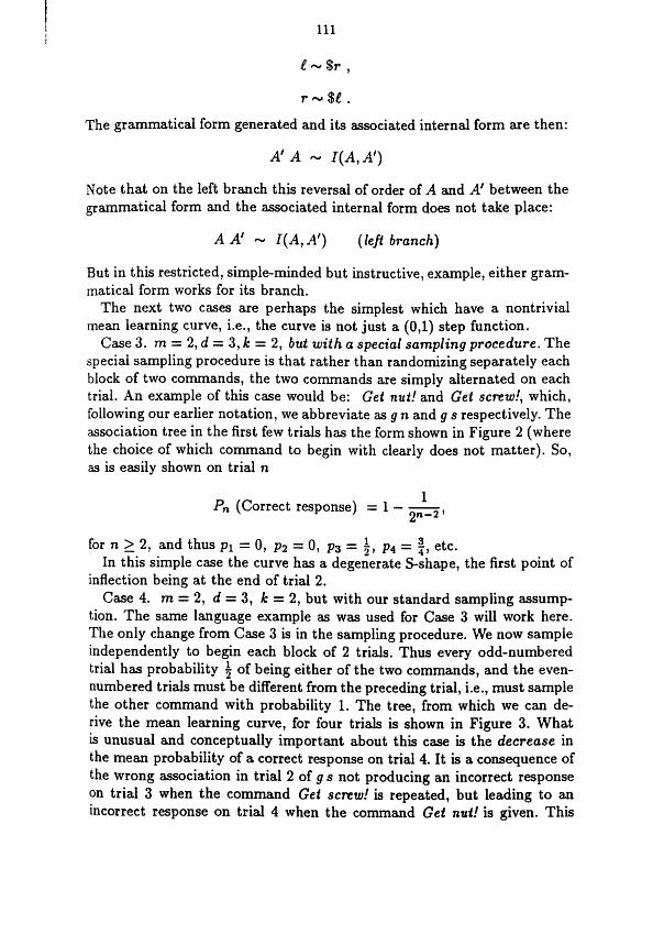
Case 3. m = 2, d = 3, k = 2, but with a special sampling procedure. The special sampling procedure is that rather than randomizing separately each block of two commands, the two commands are simply alternated on each trial. An example of this case would be: Get nut! and Gei scfezu!, which, following our earlier notation, we abbreviate as g n and g s respectively. The association tree in the first few trials has the form shown in Figure 2 (where the choice of which command to begin with clearly does not matter). So, as is easily shown on trial n

1 P,, (Correct response) = 1 - - 2"-2 '

for n 2 2, and thus p l = O, p2 = O , p3 = f, p4 = z, etc. In this simple case the curve has a degenerate S-shape, the first point of

inflection being at the end of trial 2. Case 4. m = 2, d = 3, k = 2, but with our standard sampling assump-

tion. The same language example as was used for Case 3 will work here. The only change from Case 3 is in the sampling procedure. We now sample independently to begin each block of 2 trials. Thus every odd-numbered trial has probability i of being either of the two commands, and the even- numbered trials must be different from the preceding trial, i.e., must sample the other command with probability 1. The tree, from which we can de- rive the mean leärning curve, for four trials is shown in Figure 3. What is unusual and conceptually important about this case is the decrease in the mean probability of a correct response on trial 4. It is a consequence of the wrong association in trial 2 of g s not producing an incorrect response on trial 3 when the command Get screw! is repeated, but leading to an incorrect response on trial 4 when the command Get nut! is given. This

3

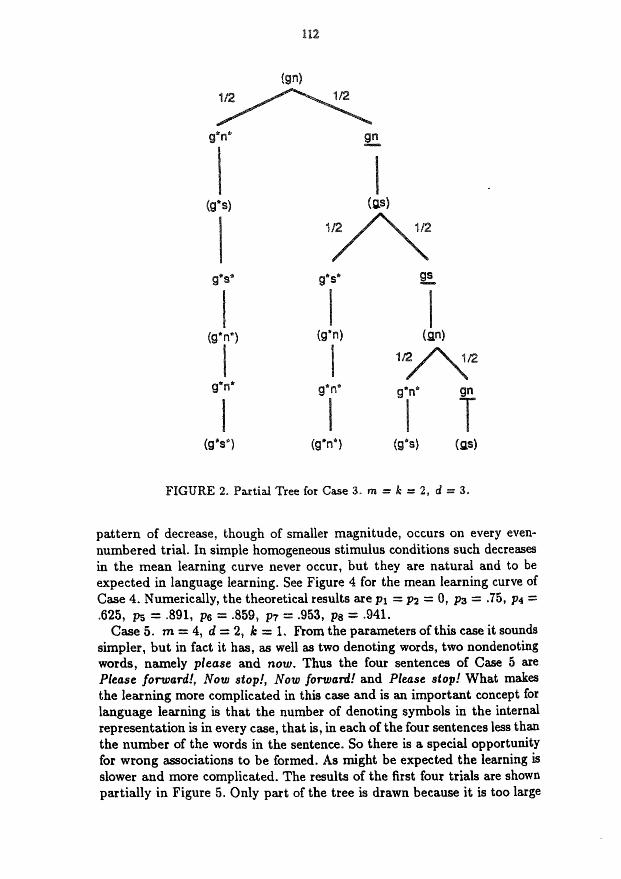
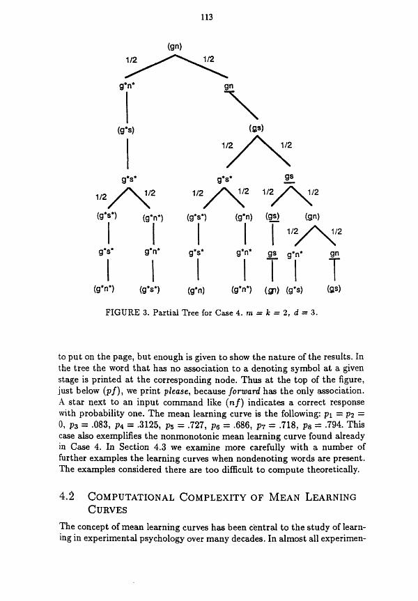
pattern of decrease, though of smaller magnitude, occurs on every even- numbered trial. In simple homogeneous stimulus conditions such decreases in the mean learning curve never occur, but they are natural and to be expected in language learning. §w Figure 4 for the mean learning curve of Case 4. Numerically, the theoretical results are p1 = p2 = O, p3 = .75, p4 =:

-625, p5 = .891, p6 = .859, p7 = .953, p8 .941. Case 5. m = 4, d = 2, k = l, From the parameters of this case it sounds

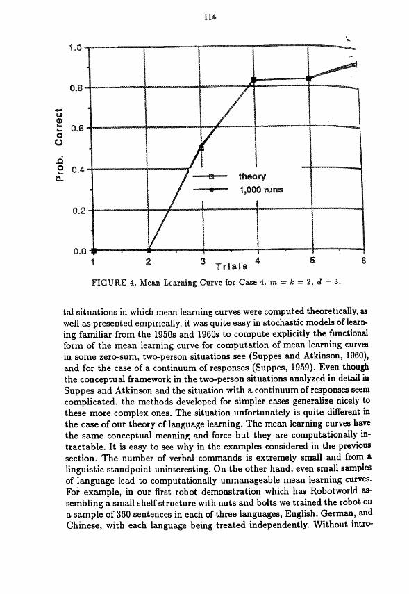
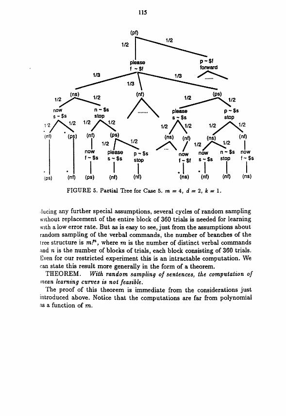
simpler, but in fact it has, as well as two denoting words, two nondenoting words, namely please and now. Thus the four sentences of Case 5 are Please forward!, Now stop!, Now forward! and Please siop! What makes the learning more complicated in this case and is an important concept fop language learning is that the number of denoting symbols in the internai representation is in every case, that is, in each of the four sentences less than the number of the words in the sentence. So there is a special opportunity for wrong associations to be formed. As might be expected the learning is slower and more complicated. The results of the first four trials are shown partially in Figure 5. Only part Q€ the tree is drawn because it is too large

113

gcs* gcs*

1 / 2 / y 1/2/y2

g's' g'n' g's' g'n'

I I f FIGURE 3. Partid Tree for Case 4. m = k = 2, d = 3.

to put on the page, but enough is given to show the nature of the results. In the tree the word that has no association to a denoting symbol at a given stage is printed at the corresponding node. Thus at the top of the figure, just below (pf), we print please, because forutad has the only association. A star next to an input command like (nf) indicates a correct response with probability one. The mean learning curve is the following: p1 = p2 =

caSe also exemplifies the nonmonotonic mean learning curve found already in Case 4. In Section 4.3 we examine more carefully with a number of further examples the learning curves when nondenoting words are present. The examples considered there are too difficult to compute theoretically.

O, p3 .083, p4 = .3125, p5 .727, p6 = ,686, p7 = .718, pa .?M. This

4.2 COMPUTATIONAL COMPLEXITY OF MEAN LEARNING CURVES

The concept of mean learning curves has been central to the study of learn- ing in experimental psychology over many decades. In almost all experimen-

i

situations in whic mean learning curves were compute well as presented empirically, it was quite easy in stochastic models of learn- ing familiar from the 1950s and 11960s to compute explicitly the functional form of the mean learning curve for computation of mean learning curves in some zero-sum, tweperson situations see (Suppes and Atkinson, 1960), and for the case of a continuum of responses (Suppes, 1959). Even though the conceptual framework in the tweperson situations analyzed in detail in Suppes and Atkinson and the situation with a continuum of responses seem complicated, the methods developed for simpler cases generalize nicely to these more complex ones. The situation unfortunately is quite different in the case of our theory of language learning, The mean learning curves have the same conceptual meaning and force but they are computationally in- tractable. It is easy to see why in the examples considered in the previous section. The number sf verbal commands is extremely small and from a linguistic standpoint uninteresting. On the other hand, even small samples of language lead to computationally unmanageable mean learning curves. For example, in our first robot demonstration which has Robotworld as- sembling a small shelf structure with nuts and bolts we trained the robot on a sample of 360 sentences in each of three languages, English, German, a d Chinese, with each language being treated independently. Without intro-

115

FIGURE 5. Partid Tree for Case 5. m = 4, d = 2, k = 1.

,lucing any further special assumptions, several cycles of random sampling wthout replacement of the entire block of 360 trials is needed for learning tuth a low error rate. But as is easy to see, just from the assumptions about random sampling of the verbal commands, the number of branches of the tree structure is m.’’’, where m is the number of distinct verbal commands and n is the number of blocks of trials, each block consisting of 360 trials. Even for our restricted experiment this is an intractable computation. We can state this result more generally in the form of a theorem.

THEOREM. With random sampling of sentences, the computation of mean learning curves is not feasible.

The proof of this theorem is immediate from the considerations just introduced above. Notice that the computations are far from polynomial as a function of m.

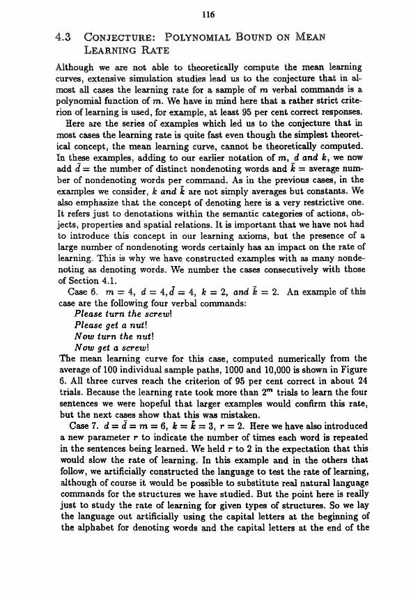
Please turn the screw! Please ge t a nut! Now turn the nut! Now get a screw!

The mean learning curve for this case, computed numerically from the average of 100 individual sample paths, 1000 and 10,000 is shown in Figure 6. All three curves reach the criterion of 95 per cent correct in about 24 trials. Because the learning rate took more than 2m trials to learn the four sentences we were hopeful that larger examples would confirm this rate, but the next cases show that this was mistaken.

Case 7. d = d = rn = 6, E = E = 3, r = 2. Here we have alm introduced a new parameter r to indicate the number of times each word is repeated in the sentences being learned. We held P to 2 in the expectation that this would slow the rate of learning. In this example and in the others that follow, we artificially constructed the language to test the rate of learning, although of course it would be possible to substitute real natural language commands for the structures we have studied. But the point here is really just to study the rate of learning for given types of structures. So we lay the language out artificially using the capital letters at the beginning of the alphabet for denoting words and the capital letters at the end of the

117

1 .o

0.8 o 2 ô * 0.6

0.2

0.0 1 1 1 2 1 31 T r i a l s

FIGURE 6. Mean Learning Curve for Case 6. m = d =d = 4, k = E = 2.

alphabet for nondenoting words. Here are the two sets of words:

d = î A B C D E F I d = Iuvwxrzl

U C Y F ! X A V E ! W B V F ! W C Z E ! X B Y D ! U A A D !

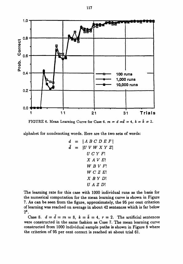
The learning rate for this case with 1000 individual runs as the basis for the numericd computation for the mean learning curve is shown in Figure 7. As can be seen from the figure, approximately, the 95 per cent criterion of learning was reached on average in about 42 sentences which is far below 26.

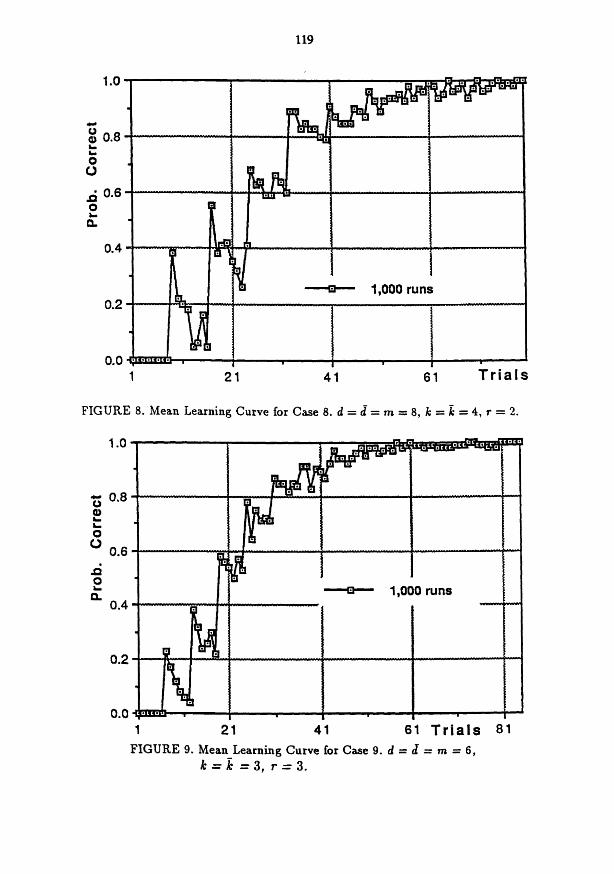
Case 8. d = 2 = m = 8, k = i = 4, r = 2. The artificial sentences were constructed in the same fashion as Case 7. The mean learning curve constructed from 1000 individual sample paths is shown in Figure 8 where the criterion of 95 per cent correct is reached at about trial 61.

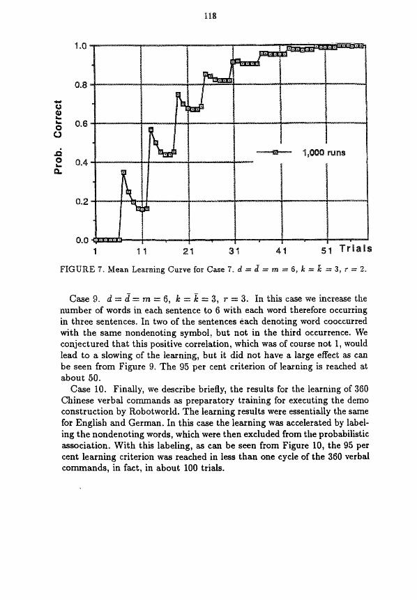
mber sf words in each sentence to three sentences. In two of the sent c o o ~ c ~ ~ ~ e

with the same nondenoting symbol, but not in the third occurrence. We conjectured that this positive correlation, which was of course not 1, would lead to a slowing of the learning, but it did not have a large effect as can be seen from Figure 9. The 95 pes cent criterion of learning is reached at about 50.

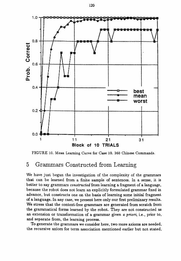
Case 10. Finally, we describe briefly, the results for the learning of 36Q Chinese verbal commands as preparatory training for executing the demo construction by Robotworld. The learning results were essentially the same for English and German. In this case the learning was accelerated by label- ing the nondenoting words, which were then excluded from the probabilistic association. With this labeling, as can be seen from Figure 10, the 95 per cent learning criterion was reached in less than one cycle of the 360 verbal commands, in fact, in about 100 trials.

119

1 21 41 61 Tr ia ls

FIGURE 8. Mean Learning Curve for Case 8. d = d = m 8, Æ = k = 4, r = 2.

1 .o

5 0.8 2 L O

o 0.6 d 2 e

0.4

0.2

0.0 1 21 $1 61 Tr ia ls 81 FIGURE 9. Mean Learning Curve for Case 9. d = d = m = 6, -

k = k = 3 , r = 3 .

I

1

FIGURE IO. Mean Learning Curve for

Ei G r m a r s Constructed from

We have just begun the investigation of the complexity of the grammars that can be learned from a finite sample of sentences. In a sense, it is better to say grammars constructed from learning a fragment of a language, because the robot does not learn an explicitly formulated grammar fixed in advance, but constructs one on the basis of learning some initial fragment of a language. In any case, we present here only our first preliminary results. We stress that the context-free grammars are generated from scratch from the grammatical forms learned by the robot. They are not constructed as an extension or transformation of a grammar given u priori, i.e., prior to, and separate from, the learning process.

TO generate the grammars we consider here, two more axioms are needed, the recursive axiom for term association mentioned earlier but not stated,

121

and the axiom of term form substitution. To make the statement explicit we need to extend the earlier discussion

of association of words with internal symbols to include terms, both of the gíven natural language and of the internal language. Formally, such associations of terms, t - r, were already used in the statement of Axioms 6, 7 and 8, but explicit explanation was given only for the special case of t being a single word, all that is essential for developments up to this point.

First, if u is an internal representation of a verbal command s, the de- noting atoms of U are just the LISP atoms that are the internai symbols associated with words of the given natural language. By a minimal LISP expression of U containing given occurrences of denoting atoms al ..., an in c we mean the smallest LISP expression, as defined at the beginning of Section 3, containing the atoms al. ..an. For example, if s Get the red screw!, and S - U = (fa1 $9 (io (f0 $r (f0 $s *)))), then there are three occurrences of denoting atoms in u, one of $g, one of $r and one of $s. The minimal LISP expression containing the one occurrence of $s in u is (f0 $s

We postulate a separate association relation for terms - separate from the association relation -, although we use the same symbol. Thus stored in memory we have

4 *

screw - (f0 $s *) for the above example, as well as scfe'w - $s stored under word associations. Also a string w of s is purely nondenoting ( d a t i v e t o s - u) iff no word of w corresponds to each occurrence of a denoting atom in 0.

Second, given a verbal command s - u and t a nonempty substring of s, the string t is a pure complete denoting term (relative to s and u) iff (i) every word of t has a corresponding association to each occurrence of a denoting atom in u, where corresponding means in accordance with the association relation s - u, (ii) the minimal LISP expression r containing the corresponding occurrences of all the denoting atoms of u associated with words of t contains no other occurrences of denoting atoms. We now use the concepts introduced to state the recursive axiom needed.

Axiom 11. (Term Assoctation). First, if a - a and a E P then a - (f0 a *). Second, if (i) awt is a substring of a verbal command s, with s - u and a - a, (ii) t is a pure complete denoting term of s with t - r , (iii) w is the substring, possibly empty, of purely nondenoting words between a and t , (i.) +(a, r ) is the minimal LISP expression of u containing the occurrences of a and denoting atoms in r corresponding to occurrences of denoting words in t and T'((Y, r )

- contains no other occurrences of denoting atoms, then awt - ~ ' ( a , r) . Moreover, the axiom applies to twa with w following t .

In the first part of the Axiom it follows from the category structure of the internal language that (f0 cy *) c O. Notice that as the axiom is for-

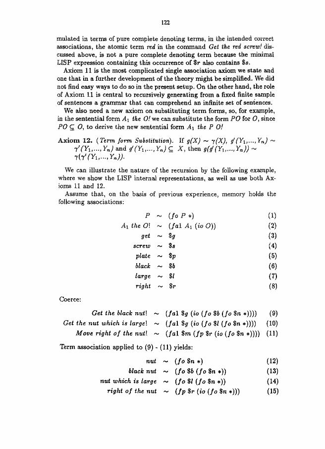
can illustrate the nature of the recurs

9 et screw plat e black large right

Coerce:

Term association applied to (9) - (11) yields:

123

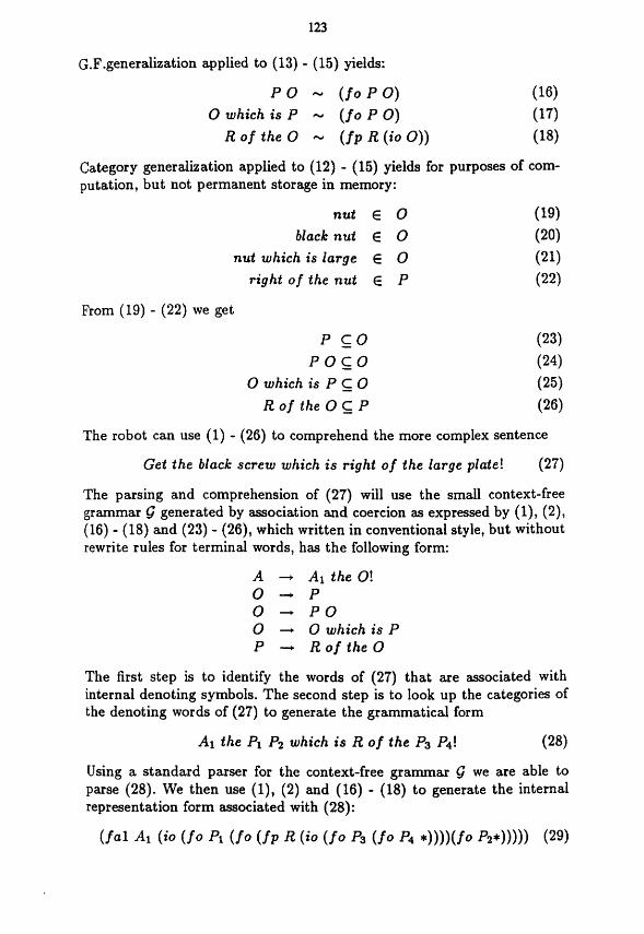
G.F.generalization applied to (13) - (15) yields:

P O - (f0 P O ) (16) O which is P - (f0 P O) (17)

R of the O - ( f p R ( io O)) (18)

Category generalization applied to (12) - (15) yields for purposes of com- putation, but not permanent storage in memory:

nut E o blad nut E O

nut which is large E O right of the nut E P

From (19) - (22) we get

P c o P O G O

O which is P s O R o f the O c P

The robot can use (1) - (26) to comprehend the more complex sentence

Get the black screw which is right of the large plate! (27)

The parsing and comprehension of (27) will use the small context-free grammar 5: generated by association and coercion as expressed by ( l ) , (2), (16) - (18) and (23) - (26), which written in conventional style, but without rewrite rules for terminal words, has the following form:

A - A1 the Q! Q - + P o - P O O - O which is P P + R o f the O

The first step is to identify the words of (27) that are associated with internal denoting symbols. The second step is to look up the categories of the denoting words of (27) to generate the grammatical form

A1 the P1 Pz which i s R o f the P3 P4! (28)

Using a standard parser for the context-free grammar G we are able to parse (28). We then use (l), (2) and (16) - (18) to generate the internal representation form associated with (28):

125

The system have both been exposed not only to English but also to structurally more remote languages such as Japanese or Chinese and Russian (our system).

Both approaches make essential use of an internal language.

Both systems require that each word has only one meaning (Siskind’s “monosemy constraint” matches our “non-ambiguity requirement”).

On the other hand, the systems are different in at least the follöwing re- spects:

1. Siskind’s systems acquire language on the basis of assertions, our system on the basis of commands.

2. Siskind’s approach appears to require a distinction between denot- ing words and non-denoting words such as determiners. Initially, our system had a similar condition but we succeeded in removing it.

3. In addition to monosemy but unlike Siskind we also require that a denotation can be expressed by only one word (our “non-synonymity constraint” of Axiom 3).

4. The output of Siskind’s system is a lexicon (list of words with syn- tactic category and meaning) in the case of MAIMRA and a lexicon together with r?-parameters of the language to be learnt in DAVRA, whereas our output is a grammar of the language to be learned.

5. As the language of conceptual representation Siskind uses a language of predicate logic without quantifiers but with variables (to handle argument relationships and arities) whereas our internal language is a variable-free procedural language.

6. Whereas our system assumes a one-one-mapping between denoting words of the verbal command and the denotations in the semantic representation (verbal input is semantically exhaustive), Siskind here can afford a more relaxed position: the verbal input can be less in- formative than the non-verbal input.

7. We start from a high-level internal representation whereas Siskind works his way up from simple state-descriptions to event-descriptions by his inference component. Siskind’s takes the bootstrapping objec- tive more seriously.

8; Siskind uses the lexical categories noun, verb, and preposition. We have carefully avoided the use of syntactic categories and have used semantic categories of action, object, property, and spatial relation instead. Of course there is a close correspondence between semantic categories and syntactic categories but there are also many examples

s

. (1990) Acquiring core meanings of words, represented as Jackendoff-style conceptual structures, from correlated streams of lin- guistic and non-linguistic input. Proceedings of the 28th Annual Meet- ing of the Assoctation of Computational Lingutstics, 143-156.

[S] Siskind, J. M. (1991a) Dispelling Myths about Language Bootstrap- ping. A A M Spring Symposium Workshop on Machine Learning of Natural Language and Ontology, Stanford.

[6] Siskind, J. M. (1991b) Naive Physics, Event Perception, Lexical Se- mantics and Language Acquisition. A A A I Spring Symposium Work- shop on Machine Learning of Natural Language and Ontology, Stan- ford.

[T] Stolcke, A. (1990) Learning Featurebased Semantics with Simple Re- current Networks. TR-90-015, International Computer Science Insti- tute, Berkeley Ca.

[s] Suppes, P. (1959) A linear model for a continuum of responses. In R. R. Bush & W. K. Estes (Eds.), Studies in mathematical learning theory. Stanford: Stanford University Press, pp. 400-414.

127