1 American Institute of Aeronautics and Astronautics

Complex-Trajectory Aerodynamics Data for Code Validation from a New Free-Flight Facility

Jeffrey D. Brown∗ and David W. Bogdanoff† Eloret Corporation, Moffett Field, CA 94035

Leslie A. Yates‡ AerospaceComputing, Inc., Mountain View, CA 94043

Michael C. Wilder§ NASA Ames Research Center, Moffett Field, CA 94035

and

Scott M. Murman¶ Eloret Corporation, Moffett Field, CA 94035

A unique new capability to obtain unsteady aerodynamics data for configurations flying complex trajectories is presented. Supersonic free-flight aerodynamics data for conical frustum-shaped projectiles were obtained in a new aero-ballistic facility at NASA Ames Research Center. The projectiles simulated insulating-foam debris shed from the Space Shuttle’s external fuel tank. The data were required by the Space Shuttle Program to validate, prior to the post-Columbia return-to-flight, the 6-DOF/CFD code used to characterize Shuttle ascent-debris aerodynamics and risks. Polyethylene frustums—nominally 3.56 cm in diameter, 0.71 cm long, and 4 grams in mass—were launched into 1-atm air at approximately M=2.8. Their rapidly-decelerating, often highly-lifting, and sometimes tumbling 6-DOF trajectories were recorded by arrays of top- and side-view ICCD cameras. The paper gives samples of the data and details of the substantial challenges and creative solutions associated with obtaining them.

Nomenclature Abbreviations and Acronyms ARC = NASA Ames Research Center CADRA = Comprehensive Automatic Data Reduction system for Aero-ballistic Ranges Cart3D = ARC cartesian-mesh, moving-boundary, fully-coupled, 6-DOF/CFD code CFD = Computation Fluid Dynamics CG = Center of Gravity DOF = Degrees of Freedom ET = Space Shuttle External fuel Tank HDPE = High Density Polyethylene HFFAF = Hypervelocity Free-Flight Aerodynamics Facility HFFGDF = Hypervelocity Free-Flight Gun Development Facility ICCD = Intensified Charge-Coupled Device LS1, LS2, … = Light-sheet detector position for panel 1, panel 2, … (see Fig. 3)

∗ Senior Research Scientist, Reacting Flow Environments Branch, MS 230-2 † Senior Research Scientist, Reacting Flow Environments Branch, MS 230-2, Associate Fellow AIAA ‡ Vice President, 465 Fairchild Drive, Suite 224, Senior Member AIAA § Aerospace Engineer, Reacting Flow Environments Branch, MS 230-2, Senior Member AIAA ¶ Senior Research Scientist, Applications Branch, MS T-27 B, Member AIAA

2 American Institute of Aeronautics and Astronautics

PTG = Programmable Timing Generator RMS = Root Mean Squared STS = Space Transportation System S1, S2, … = Side-view camera position for panel 1, panel 2, … (see Fig. 3) T1, T2, … = Top-view camera position for panel 1, panel 2, … (see Fig. 3) Variables and Parameters Ixx, Iyy, Izz = model moments of inertia (Table 1); z is radial axis of symmetry for shots 8 – 21 t = time V, Vavg, V0 = velocity, average velocity, initial velocity x, y, z = facility coordinates in axial, transverse, and vertical direction xcg, ycg, zcg = CG coordinates measured from center of (symmetric) model base (Table 1) ytot, ztot = cross-range travel in y, z direction, measured at witness sheet or point of wall impact (Table 1) θ, ψ = model angle relative to facility floor (nominal pitch), side-wall (nominal yaw)

I. � Introduction HIS paper introduces to the aerospace aerodynamics community a unique experimental capability at the NASA Ames Research Center (ARC) to obtain valuable six degree-of-freedom (6-DOF) data for projectiles flying

complex trajectories. Further, it presents a set of such data that were acquired for conical frustum-shaped models, which simulated Space Shuttle external fuel tank (ET) insulating-foam debris, rapidly decelerating from M=2.8. The complete data set and the full details of the experimental facility and approach will be provided in a subsequent publication.1 In the next section of this paper, the need to obtain the data is discussed as background. Subsequent sections present the facility and various aspects of the test methodology, each as it represented an innovative solution to one or more formidable technical challenges imposed by the experimental requirements. Representative data are shown in a separate section on results, followed by a discussion of error analysis. We conclude that this work resulted both in a very successful test and exciting new assets for continued research.

II. � Background Following the loss of Columbia (STS-107) in 2003, NASA mandated that the full Space Shuttle ascent-debris environment, and the risks it posed to the vehicle and crew, be characterized. In this computationally-driven process, numerous debris sources, such as ET insulating foam, were first identified. For each source, likely debris geometries, masses, aerodynamic properties, and release (i.e., initial flight) conditions were input to a debris transport analysis code,2 which calculated families of debris trajectories. From these, the hazards associated with debris impacts on the Shuttle orbiter were assessed.

In order to operate with the speed required by its purpose, quickly calculating hundreds of thousands of debris trajectories, the debris transport analysis code incorporates several simplifications of the physical problem. A drag model applied in the direction of the local flow velocity determines the debris decelerations and zero-lift trajectories, thus the energies of potential impacts. Meanwhile, empirically derived containment cones, reflecting the debris cross-range, or lifting, characteristics are applied to the zero-lift trajectories to reveal the possible impact locations.

The drag models and containment cones used in the debris transport analyses were produced through an automated computational fluid dynamics (CFD) process developed at ARC.3 The process, referred to here as Cart3D, applied individual Cartesian-mesh, fully-coupled, 6-DOF/CFD debris-trajectory simulations in a Monte Carlo fashion to identify the aerodynamic behaviors of numerous debris shapes and shedding scenarios.2

In late 2003, NASA ordered that, prior to return-to-flight (RTF), the Cart3D process and the foam-debris aerodynamics derived through it be validated against experimental data. (Following Columbia, ET insulating foam was the debris source of greatest concern.) After an unsuccessful search for existing data that were geometrically and dynamically relevant to the problem, computational and experimental teams at ARC joined together and devised a series of free-flight tests to provide them.

The tests had three principal objectives. The first priority was to determine whether a symmetric frustum model released at the estimated flight Mach number would tend to oscillate about a stable trim point as it decelerates or simply tumble. Cart3D predictions pointed to the former case, which, because it would incur much higher aerodynamic drag than the latter, forced NASA to plan for higher potential debris-impact energies than it otherwise would have. Assuming the symmetric models did trim rather than tumble, the second experimental priority was to obtain trajectory data for them, over 1.5 to 2 oscillation cycles, covering a range of oscillation amplitudes. These data would be used to validate the physics in, and the drag models derived from Cart3D. The final objective was to

T

3 American Institute of Aeronautics and Astronautics

record as broad a spectrum as possible of lifting trajectories, using asymmetric models. The envelope of those trajectories (e.g., on a plot of cross-range vs. axial distance) could then be compared with the one obtained through the computational Monte Carlo process.

III. � Finding/Creating The Test Facility The question whether symmetric frustums tended to oscillate or tumble was only relevant over a short length

scale in flight, namely the distance between a debris pop-off location on the Shuttle ET and a strike point on the orbiter. For a given initial angular rate, if a debris piece is to tumble, the ratio of its density to that of the air will affect how quickly it does. Therefore, for code validation, it was required that the experimental test conditions be dynamically similar to flight. That is, for tests at the flight Mach number,

(ρmodel/ρair-test) = (ρfoam/ρair-flight).

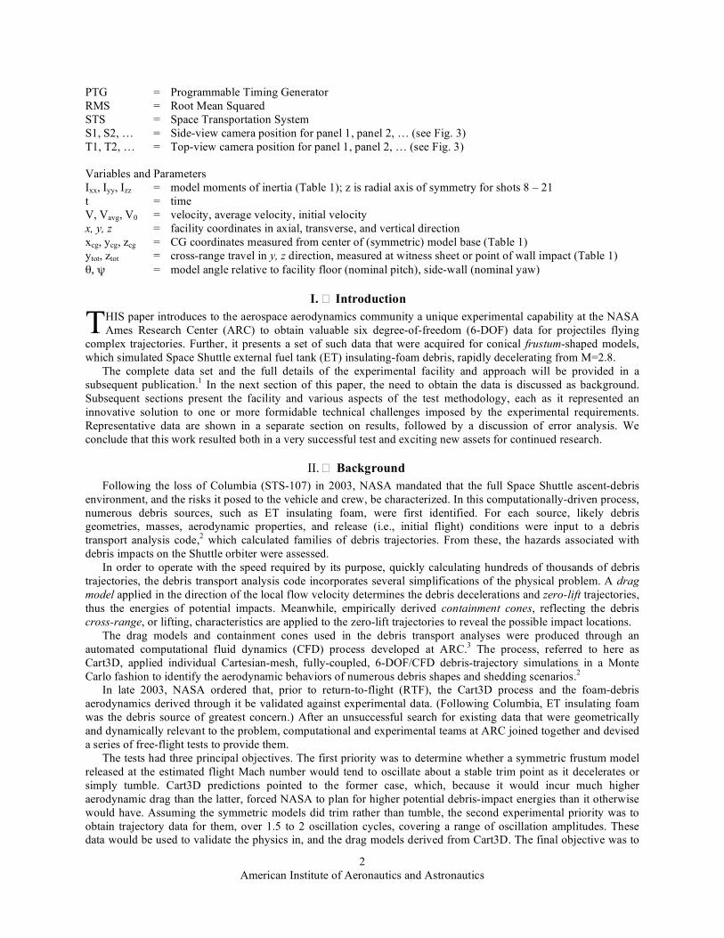
Ballistic range aerodynamics tests have not generally been used to simulate these kinds of rapidly-decelerating, imposed-length-scale trajectories, and dynamic similarity is not a typical requirement. The density ratio between insulating foam and air at the estimated flight pop-off altitude is very small (~700) relative to that for, say, an Earth entry vehicle that might be the subject of a standard free-flight range test. Still, by testing at 1 atm pressure (the maximum achievable in the known available facilities), and using projectiles made from a light plastic (e.g., polyethylene), the ratio could nearly be matched, and dynamic similarity obtained. A bigger problem was that in all of the known facilities, a significant distance separated the gun muzzle from the first data station. At atmospheric pressure, this would result in the light, high-drag (i.e., low ballistic coefficient), and (for some) high-lift frustum models decelerating to a subsonic velocity and possibly swerving out of the field of view before any data were acquired. The Ames Hypervelocity Free Flight Aerodynamics Facility (HFFAF), shown in Fig. 1, offered a possible solution. In this facility, the space between the gun and the test section is enclosed by a pressure vessel, called the separation (or dump) tank, which can be evacuated to zero pressure. If the facility were modified to allow placement of a thin, replaceable diaphragm at the flange (just visible at the far right in Fig. 1) joining the dump tank to the test section, the former could be kept at vacuum while the latter remained at atmospheric pressure. Therefore, the model would only begin to decelerate (and lift) after breaking through the diaphragm and entering the test section. With this innovation, the HFFAF could overcome the problem of the initial, gross model deceleration and swerve. However, another problem remained that could not be surmounted. The HFFAF only allows for a single data sample (shadowgraph) per optical station, and the distance between stations is over 1.5 m. That distance and the relatively small (30.5 cm-diameter) windows would be prohibitive to obtaining data capable of reproducing the trajectories of such rapidly decelerating, rotating, and lifting projectiles. The reality was that the test requirements demanded a Mach-three-capable free-flight facility, with an expansive test section that provided near-continuous optical access, in which the projectile could be prevented from decelerating or changing path before reaching the

Figure 1. Ames HFFAF test section with side shadow graph cameras (red boxes).

Figure 2. HFFGDF schematic.

4 American Institute of Aeronautics and Astronautics

initial data-acquisition point. Unfortunately, no such facility existed. The good news was that we had immediate access to a significant head start in constructing one. The Ames Hypervelocity Free-Flight Gun Development Facility (HFFGDF), which resides in the same ballistic range complex as the HFFAF, was designed for developing projectile launchers and launching techniques. It was not an aerodynamics facility. It had no test section. Still, it possessed virtually the same gun mount and separation tank, with the same vacuum system, as the HFFAF. And on that foundation, we were able to construct the facility we needed to support Shuttle-debris tests, a new HFFGDF. The basic (new) facility, shown schematically in Fig. 2, includes a gun, separation tank, test section (or optical range), and model catcher. The gun, which is changeable, was a 4.41 cm-diameter smooth-bore powder gun capable of launch velocities between M = 1 and M = 4.5. The 10.1 meter-long dump tank, which contains a conical, steel sabot stripper, was sealed at the down-range end with a thin Mylar diaphragm and evacuated prior to each shot. The model catcher at the down-range end of the test section consists of twelve vertically-hung 1.3 cm-thick felt sheets. The main feature of the new HFFGDF is the 4.9 m-long, 2.0 m-high, 1.8 m-wide atmospheric test section, comprised of sixteen transparent, 1.3 cm-thick polycarbonate (Lexan) panels. The panels are supported and held together by a steel frame. Three orthogonal-view drawings of the test section and an end-view photograph are shown in Fig. 3. In Fig. 3d, one sees the yellow separation tank and the 20 cm-diameter orifice (at the center of its gray end flange) through which the model enters the test section. In the axial direction, the optical range is divided into four panels, or bays, each nominally 1.2 m long. With its transparent walls and large interior, the test section allows for the frequent and extended optical sampling necessary to track the high oscillation-rate, large cross-range model trajectories we expected to see.

a)

b) c)

d)

Figure 3. HFFGDF test section, a) top view, b) side view, c) end view, d) opposite end view

5 American Institute of Aeronautics and Astronautics

IV. Choosing the Models and a Different Sabot Based on earlier experiments to investigate the shapes of foam debris,2 the nominal, or baseline (symmetric)

projectile geometry chosen for the current test was a conical frustum (see Fig. 4) with a base diameter of 3.56 cm, a base angle of 40 degrees, and a length-to-diameter ratio of 0.2.

For cross-range testing, two types of asymmetric models were used: those that were weighted and those that were sliced. For each type, two variations – one with less asymmetry (aluminum weighted and 30-deg. sliced) and one with more (brass weighted and 18-deg. sliced) – were launched. The four varieties are shown in Fig. 5, along with the nominal case. All of the projectiles were constructed from high density polyethylene (HDPE). Their designs were a matter of particularly close collaboration between the experimental and CFD teams.

The models were launched inside sabots made of acrylonitrile butadiene styrene (ABS) plastic. The cylindrical sabots were cut lengthwise into quarters, or fingers, and the internal faces were serrated so that they locked firmly together inside the gun barrel.

Normally, in free-flight testing with saboted models, aerodynamic forces up-range of the test section separate the sabot from the model.4 As the launch package emerges from the gun, pressure forces against the sabot’s ramped inner-front surface (see Fig. 6b) push the fingers far enough outward from the model that they can be physically blocked from entering the test section without impeding the flight of the model. In the HFFGDF, this is done by the outside surface of the steel stripper cone, keeping the sabot parts in the dump tank, while the model passes through the cone’s 7.6 cm-diameter center-bore.

For the present experiment, with a vacuum required in the dump tank, aerodynamic sabot separation was not an option. Instead, we employed an unconventional rear-separation technique5 that uses the muzzle blast to pressurize a cavity in the rear of the sabot (see Fig. 6c) as the launch package leaves the gun. The radial forces inside the cavity

Figure 4. Baseline, conical frustum model.

a) b) Figure 5. Asymmetric models; a) weighted, b) sliced.

a) b) c) Figure 6. Models and sabots; a) baseline model, b) launch assembly front end, c) sabot rear cavity.

6 American Institute of Aeronautics and Astronautics

push the sabot fingers apart. The cavity’s depth and diameter were chosen to gain enough radial force to move the sabot fingers outboard of the stripper bore while still ensuring the sabot’s structural integrity during launch. Further details on the sabot design are given in Ref. 1.

V. � Devising the Data Acquisition System As the HFFGDF had not previously been an aerodynamics range, it had no trajectory-data acquisition system.

There was neither time nor budget to construct a fixed-location shadowgraph system, like the one in the HFFAF. And, more importantly, it was not suitable for the complex, unpredictable model trajectories we anticipated. We needed a means to capture – for each shot, nearly anywhere in the test section – many short-duration exposures (on the order of 1 µs, to “freeze” the projectile motion) of a rapidly-moving model. Furthermore, the resolution of the individual exposures – acquired in low light, relative to the high-voltage spark-source-illuminated shadowgraphs – had to be high enough to allow the instantaneous positions and angles to be determined.

Our solution came through the innovative use of several digital, intensified charge-coupled device (ICCD) cameras. The cameras, shown in Fig. 7 with their programmable timing generator (PTG) controllers, had only been used at ARC for single-exposure thermal and spectroscopic imaging. However, they could also be operated in a high-frequency burst mode, where several sequential exposures, or bursts, could be loaded onto a single CCD-array image before its contents were transferred to a computer (or other storage device) or erased. In this way, the trajectory of an illuminated white model moving in front of a black background could be captured in several discrete exposures as it traversed the camera’s field of view. In terms of aerodynamics data, one camera could be the equivalent of many shadowgraph stations.

Each side and top view camera was positioned on an axis passing approximately through the center of a test section bay, as diagrammed in Fig. 3. For testing the baseline models, six cameras were used to record top and side views of the first three bays. A seventh camera was added for testing the asymmetric models. The arrangement was as shown in Fig. 3; all views were provided except the top of panel 2.

The lenses and positions chosen for the cameras were to give approximately a 1.3 x 1.3 m field of view at the center of the range, slightly longer than an individual bay. This resulted in the model diameter being resolved into approximately 14 pixels by the 512 x 512 pixel CCD arrays. We believed from experience that this was sufficient to provide reasonably accurate measurements of the projectile position and angles.

The camera burst intervals were set, from 120 µs up to 216 µs, according to where they were located; the objective was to fill the field of view as completely as possible with up to 14 exposures of the model. Much shorter intervals, therefore, more model exposures per image, were possible. However, with more than 14 bursts, the accumulated light on the black background began to reduce the contrast with the model enough to degrade the measurement accuracy.

The ICCD cameras were triggered by infrared ballistic light screens (or sheets) that sensed the passage of the projectiles and emitted a trigger pulse to the PTGs. The positions of the light sheets are noted in the Fig. 3 drawings; they are clearly visible in Fig. 3d.

Seconds prior to each shot, sixteen 1 kW incandescent lamps, located along the north upper corner of the test section, and five 1 kW spot lights, positioned at the ends (see Fig. 3), were energized to illuminate the optical range. Some of the lamps are visible in the upper left of Fig. 3d, however the spot lights do not appear.

At the bottom and to the right in Fig. 3d are the calibration grids. They provided the required scale, position, and orientation information for determining the model location and angles. The grids were covered with black background cloth for each shot. They are discussed further in the section on data reduction, below.

Reference 1 discusses the full data acquisition system and the acquisition procedure in greater detail.

Figure 7. ICCD cameras (on tripods) and PTG controllers (on floor).

7 American Institute of Aeronautics and Astronautics

VI. � Reducing and Analyzing the Data Figure 8 shows an example of the raw data provided by the ICCD cameras. The photographs are the top- and

side-view, multiple-exposure images of a single projectile flying across bay 2 of the optical range. The two cameras that took them were set for the same burst frequency and triggered simultaneously by the light sheet, LS2.

The Comprehensive Automatic Data Reduction system for Aero-ballistic Ranges, CADRA,6 was used to identify the position and orientation of the projectiles and other objects (i.e., fiducial grid lines and calibration items) contained in the camera images. CADRA automatically identifies all pixels in the image associated with the object.

a)

b) Figure 8. Raw data frames from shot 5, panel 2, a) top and b) side views: burst interval = 140 µs; Vavg = 650 m/s; motion is from left to right.

a) b) Figure 9. Schematic for determination of model a) position and b) orientation.

8 American Institute of Aeronautics and Astronautics

It then uses this information and the gray-scale values for each pixel to calculate the centroid and symmetry axis of the object. Several methods are available within CADRA to transform the centroid to the center-of-gravity location.

The position of the model was defined, as illustrated in Fig. 9a, by the nearest point to two lines, one connecting the side-view camera to the projection of the model image on the side-wall fiducial grid, and the other connecting the top-view camera to the model image projection on the floor grid. The model orientation was designated, as shown in Fig. 9b by the intersection of two planes; the first plane was formed by the side-view camera and the projection of the model axis on the side-wall grid, while the second derives from the top-view camera and the projection of the model axis on the floor grid.

The images of the grids provided the required scale, position, and orientation information for determining the model position and attitude. The grid lines were 0.79 cm wide (roughly 2 pixels for the given optical set-up) and were spaced 15.24 cm (6 in.) apart. The first step in generating the functions for transforming pixel measurements to position and orientation measurements was to identify and locate all the lines in the grid images using CADRA. This process, the details of which are given in Ref. 1, showed the average errors in grid spacing to be 0.04 cm for the vertical lines and 0.08 cm for the horizontal.

To minimize the measurement uncertainty of the model position and orientation for the given optical and lighting set-ups, we needed to know the precise locations of the cameras relative to the grids, and of the grids relative to each other. A facility calibration procedure, in which the known approximate locations of the cameras and grids were refined within CADRA, was used for this purpose. In the calibration procedure, images were taken of objects with precisely-known dimensions and shapes – e.g., the barbell, a steel rod with aluminum disks at each end, in Fig. 10 – at several locations within the optical range, chosen to provide full coverage of the viewing area. Then, the camera positions and the relative positions and orientations of the grids, parameters in CADRA, were adjusted until the errors in the calculated object dimensions were minimized.

Separate calibration objects were used for images within individual test-section bays, between two bays, and over the entire test section. The measured model trajectories were also used to remove any disjointedness between bays left by the calibrations. If the indicated motions between two panels were disjointed, the camera locations and grid positions and orientations were refined within CADRA to obtain the desired smoothness.

Three full calibrations were performed during the experiment: one prior to the start of testing; the second, when the camera configuration was changed to allow for cross-range testing; and the third after the experiment was completed. The grids were also photographed immediately before and following each shot, to check whether any of the cameras or grids had been inadvertently moved. The photos showed that no accidental movement had occurred, and no additional calibrations were required.

VII. The Results Table 1 lists the key model parameters, atmospheric (i.e., test section) conditions, and initial Mach numbers for

the 20 shots (of 21 tried) that yielded trajectory data. It also shows the RMS pitch and yaw angles and, for the asymmetric models, the cross-range distances traveled in the horizontal and vertical directions (over the length of the range), and their resultant (total swerve). The coordinate system is right handed, as shown in Fig. 9, with the origin on the gun axis, at the entrance to the optical range (i.e., the center of the diaphragm). The swerves were measured, except for three shots, on a butcher-paper witness sheet placed in front of the model catcher, 5.35 m from the diaphragm. In shots 10, 14, and 16, the models lifted so strongly that they failed to reach the end of the range before impacting one of the four sides. The swerves listed for them were measured at the points of impact, where

Figure 10. Calibration barbell atop tripod.

9 American Institute of Aeronautics and Astronautics

visible marks were made, and the corresponding axial locations are noted just below Table 1. The table also contains information on how the models were loaded in the gun (i.e., whether, for the asymmetric models, the inserts or thin edge was oriented up, down, or at an angle) and how, if at all, the projectiles were tripped, or kicked, inside the dump tank. The latter was done, by placing a thin material (usually aluminum foil) eccentrically in the model’s path, to produce larger model oscillations.

Examples of the trajectory data for the symmetric models are shown in Fig. 11. None of the eight baseline projectiles tumbled; rather, they all oscillated about a stable trim point as they flew down the range, very close to the gun axis. Even shot 6, with oscillation amplitudes of over ±80 degrees in pitch and ±45 degrees in yaw, did not tumble.

Figure 12 shows sample trajectories for each of the 4 types of asymmetric models. In general, the aluminum insert models exhibited no more average lift than did the baseline projectiles. However, their oscillation amplitudes, un-kicked, were significantly larger. The brass-insert and 18-degree sliced models showed a very stable tendency to lift strongly, the latter even more than the former. Figure 12c, for the 18-degree model, reveals a highly-damped pitch oscillation about a trim angle of approximately -45 degrees and a very strong lifting behavior. For the 30 degree-slice cases, the cross-range motion was less predictable. For two of the 30-degree shots, 12 and 13, the model entered the test section facing backwards but stabilized to a forward facing motion. In shot 17, the motion appeared to be neutrally stable, but the model tumbled in shot 15. The model emerged from the dump tank in shot 14 with its back face pointing forward, and it flew that way for the length of the test section, without any indication that it would tumble or turn around. For the forward facing and tumbling models, the total cross-range motion was relatively small, between 15 and 30 cm. For the backward facing model, however, it was much larger, similar to the 18-degree models.

Figure 13 shows the one-to-one comparison between the trajectory data of a model that underwent medium-amplitude pitch and yaw oscillations (shot 5) and the Cart3D predictions started from similar initial conditions. In Fig. 14, a comparison is given between the predicted and observed drag behaviors for a range of projectile oscillation amplitudes. The figures taken together provide considerable confidence in the ability of the Cart3D code to model the aerodynamic drag forces on foam debris correctly.

In Fig. 15, the spectrum of cross-range behaviors observed in the experiment is overlaid on that predicted by the Cart3D Monte Carlo analysis. There is very good agreement. The initial conditions used in the Monte Carlo calculations were determined primarily from Shuttle launch and other, experimental data; they were applied randomly, and there were many more of them than could be represented in the ballistic range test. The good agreement between the data and Cart3D predictions, therefore, leads us to believe that, 1) the lifting behaviors observed in the test represent a realistic cross-section of those to be expected in flight, and 2) significant confidence can be placed in Cart3D’s ability to model them.

Table 1. HFFGDF Shot Summary.

10 American Institute of Aeronautics and Astronautics

a) b)

c) d)

Figure 11. Baseline-model trajectory data for shots a) 2, b) 3, c) 4, and d) 7.

11 American Institute of Aeronautics and Astronautics

a) b)

c) d) Figure 12. Asymmetric-model trajectory data for shots a) 8 – aluminum insert, b) 21 – brass insert, c) 19 – 18 degree slice, and d) 17 – 30 degree slice.

12 American Institute of Aeronautics and Astronautics

a) c) Figure 13. CFD vs. experiment; a) axial position vs. time, b) yaw angle (ψ) vs. time, c) pitch angle (θ) vs. time.

a) b) c) Figure 14. CFD drag (position) prediction vs. data; a) small oscillation amplitude, b) large oscillation amplitude, c) medium oscillation amplitude.

Figure 15. Cross-range behavior: experiment vs. CFD.

13 American Institute of Aeronautics and Astronautics

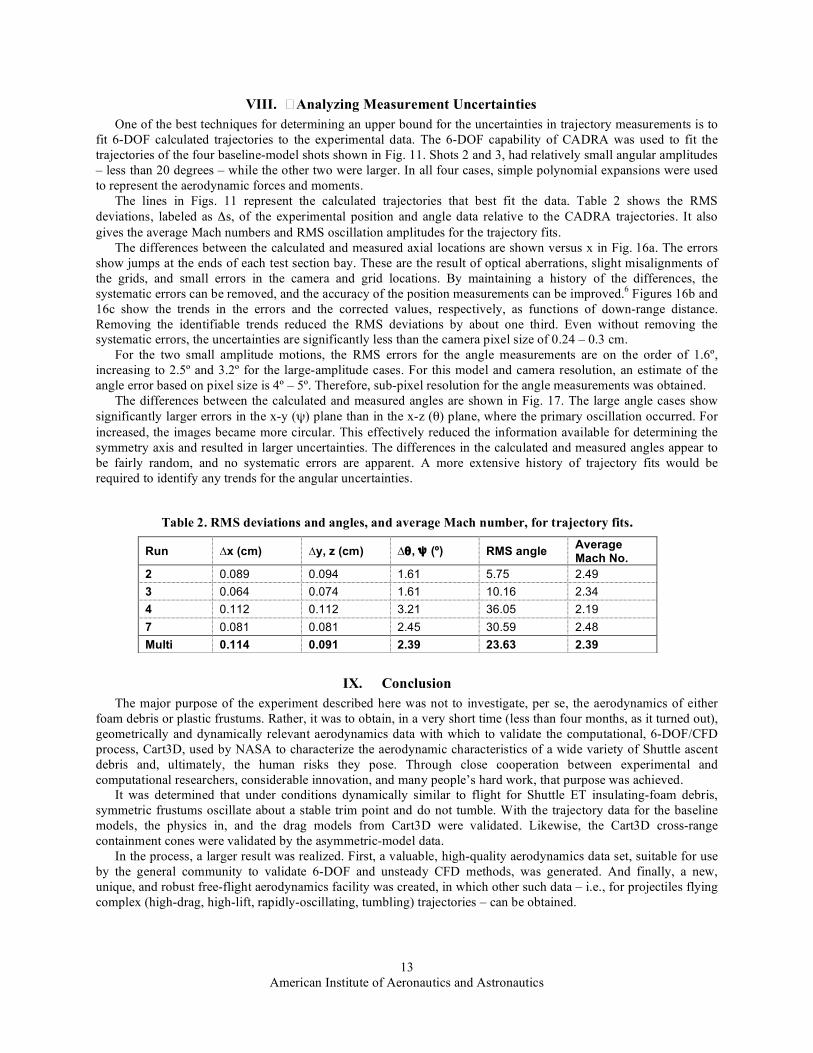
VIII. � Analyzing Measurement Uncertainties One of the best techniques for determining an upper bound for the uncertainties in trajectory measurements is to

fit 6-DOF calculated trajectories to the experimental data. The 6-DOF capability of CADRA was used to fit the trajectories of the four baseline-model shots shown in Fig. 11. Shots 2 and 3, had relatively small angular amplitudes – less than 20 degrees – while the other two were larger. In all four cases, simple polynomial expansions were used to represent the aerodynamic forces and moments.

The lines in Figs. 11 represent the calculated trajectories that best fit the data. Table 2 shows the RMS deviations, labeled as Δs, of the experimental position and angle data relative to the CADRA trajectories. It also gives the average Mach numbers and RMS oscillation amplitudes for the trajectory fits.

The differences between the calculated and measured axial locations are shown versus x in Fig. 16a. The errors show jumps at the ends of each test section bay. These are the result of optical aberrations, slight misalignments of the grids, and small errors in the camera and grid locations. By maintaining a history of the differences, the systematic errors can be removed, and the accuracy of the position measurements can be improved.6 Figures 16b and 16c show the trends in the errors and the corrected values, respectively, as functions of down-range distance. Removing the identifiable trends reduced the RMS deviations by about one third. Even without removing the systematic errors, the uncertainties are significantly less than the camera pixel size of 0.24 – 0.3 cm.

For the two small amplitude motions, the RMS errors for the angle measurements are on the order of 1.6º, increasing to 2.5º and 3.2º for the large-amplitude cases. For this model and camera resolution, an estimate of the angle error based on pixel size is 4º – 5º. Therefore, sub-pixel resolution for the angle measurements was obtained.

The differences between the calculated and measured angles are shown in Fig. 17. The large angle cases show significantly larger errors in the x-y (ψ) plane than in the x-z (θ) plane, where the primary oscillation occurred. For increased, the images became more circular. This effectively reduced the information available for determining the symmetry axis and resulted in larger uncertainties. The differences in the calculated and measured angles appear to be fairly random, and no systematic errors are apparent. A more extensive history of trajectory fits would be required to identify any trends for the angular uncertainties.

IX. Conclusion The major purpose of the experiment described here was not to investigate, per se, the aerodynamics of either

foam debris or plastic frustums. Rather, it was to obtain, in a very short time (less than four months, as it turned out), geometrically and dynamically relevant aerodynamics data with which to validate the computational, 6-DOF/CFD process, Cart3D, used by NASA to characterize the aerodynamic characteristics of a wide variety of Shuttle ascent debris and, ultimately, the human risks they pose. Through close cooperation between experimental and computational researchers, considerable innovation, and many people’s hard work, that purpose was achieved.

It was determined that under conditions dynamically similar to flight for Shuttle ET insulating-foam debris, symmetric frustums oscillate about a stable trim point and do not tumble. With the trajectory data for the baseline models, the physics in, and the drag models from Cart3D were validated. Likewise, the Cart3D cross-range containment cones were validated by the asymmetric-model data.

In the process, a larger result was realized. First, a valuable, high-quality aerodynamics data set, suitable for use by the general community to validate 6-DOF and unsteady CFD methods, was generated. And finally, a new, unique, and robust free-flight aerodynamics facility was created, in which other such data – i.e., for projectiles flying complex (high-drag, high-lift, rapidly-oscillating, tumbling) trajectories – can be obtained.

Table 2. RMS deviations and angles, and average Mach number, for trajectory fits.

Run ∆x (cm) ∆y, z (cm) ∆θ, ψ (º) RMS angle Average Mach No.

2 0.089 0.094 1.61 5.75 2.49 3 0.064 0.074 1.61 10.16 2.34 4 0.112 0.112 3.21 36.05 2.19 7 0.081 0.081 2.45 30.59 2.48 Multi 0.114 0.091 2.39 23.63 2.39

14 American Institute of Aeronautics and Astronautics

a)

b)

c)

Figure 16. Down-range uncertainties: a) uncorrected, b) uncertainty trends, c) with trends removed

-10.0

-8.0

-6.0

-4.0

-2.0

0.0

2.0

4.0

6.0

8.0

10.0

0.0 1.0 2.0 3.0 4.0

x (m)

!! (

°)

Run 002 Run 003

Run 004 Run 007

a)

-10.0

-8.0

-6.0

-4.0

-2.0

0.0

2.0

4.0

6.0

8.0

10.0

0.0 1.0 2.0 3.0 4.0

x (m)

!!

(°)

Run 002 Run 003

Run 004 Run 007

b) Figure 17. Differences between measured and calculated angles in the a) x-z plane and b) x-y plane

15 American Institute of Aeronautics and Astronautics

Acknowledgments A mere mention of names is inadequate in conveying the importance to this project of the many people involved. This work was carried out under a very demanding schedule, dictated by NASA’s movement toward returning the Space Shuttle to flight, and it involved many last-minute design and plan changes. That schedule and those changes applied as much (at times more) to the facility crew, the machinists, and others as they did to the authors.

We very gratefully acknowledge, from NASA Ames, Don Holt, Don Bowling, Rick Smythe, and Chuck Cornelison for their free-flight testing expertise, their flawless preparation and operation of the facility, and their major contributions to the design and assembly of the HFFGDF test section; Jorge Rios and Jean-Pierre Wiens for key assistance in the design and set-up of the photometric aspects of the experiment, critical day-to-day operational support, and project photo-documentation; Jim Scott, Jim Freel, John Torres, Frank Larsen, Steve Cunningham, and Mike Frediani for expert fabrication of all models, sabots, and facility components, design help, and adaptability to multiple design changes and a very demanding schedule; Jose Chavez-Garcia for assistance in experimental design and set-up; Bob Kruse, Bob Miller, and Jas Taunk for measuring all model and sabot mass properties, bringing the GDF X-ray camera system back into operation, and critically-timed design support, respectively; Jim Gavorko and Steve Nance for large-scale machining and other badly-needed support; and Michael Aftosmis and Stuart Rogers for help in the guiding the original project and consultations during it. From outside of Ames, we acknowledge Dave Moir of DOE/LANL and Randy Reiger of Roper Scientific, for very generous, extended loans of critically-needed equipment; and, from NASA/JSC, Ricardo Machin, Ray Gomez, and Bob Ess, for their continuous help, interest, and support.

Support for this work by NASA contracts No. NNA04BC25C and No. NAS2-00062 to Eloret Corporation is also gratefully acknowledged.

References 1Bogdanoff, D.W., Brown, J.D., Yates, L.A., and Wilder, M.C., “An Experimental Study of Space Shuttle Ascent Debris

Aerodynamics in the NASA Ames Research Center Ballistic Range,” NASA Technical Memorandum, to be published 2006. 2Murman, S. M., Aftosmis, M. J. and Rogers, S. E., “Characterization of Space Shuttle Ascent Debris Aerodynamics Using

CFD Methods,” AIAA Paper 2005-1223, Jan. 2005 3Murman, S.M., Aftosmis, M.J., and Berger, M.J., “Simulations of 6-DOF Motion with a Cartesian Method,” AIAA Paper

2003-1246, Jan. 2003. 4Canning, T. N., Seiff, A. and James, C. S., “Ballistic-Range Technology,” AGARDograph No. 138, August 1970, Ch. 3. 5Francesconi, A. and Pavarin, D., “Sabot Techniques for CISAS LGG,” CISAS UNIPD Internal Report, University of

Padova, Italy, 2005. 6Yates, L., CADRA System User Guide, AerospaceComputing, Inc., 1995. 7Holt, D.M., “Proof-of-Principle High Speed Electronic Imaging System - Phase II,” AFATL-TR-85-065, Dec. 1987. 8Kittyle, R.L., Packard, J.D., and Winchenbach, G.L., “Description and Capabilities of the Aeroballistic Research Facility,”

AFATL-TR-87-08, May 1987.