Embed Size (px)
Citation preview

Copyright © 2009 Pearson Addison-Wesley 8.1-1
8Complex Numbers, Polar Equations, and Parametric Equations

Copyright © 2009 Pearson Addison-Wesley 8.1-2
8.1 Complex Numbers
8.2 Trigonometric (Polar) Form of Complex Numbers
8.3 The Product and Quotient Theorems
8.4 De Moivre’s Theorem; Powers and Roots of Complex Numbers
8.5 Polar Equations and Graphs
8.6 Parametric Equations, Graphs, and Applications
8Complex Numbers, Polar Equations, and Parametric Equations

Copyright © 2009 Pearson Addison-Wesley 1.1-38.1-3
Complex Numbers8.1Basic Concepts of Complex Numbers ▪ Complex Solutions of
Equations ▪ Operations on Complex Numbers

Copyright © 2009 Pearson Addison-Wesley 8.1-4
Basic Concepts of Complex Numbers
i is called the imaginary unit.
Numbers of the form a + bi are called complex
numbers.
a is the real part.
b is the imaginary part.
a + bi = c + di if and only if a = c and b = d.

Copyright © 2009 Pearson Addison-Wesley 1.1-58.1-5
Copyright © 2009 Pearson Addison-Wesley 8.1-6
Basic Concepts of Complex Numbers
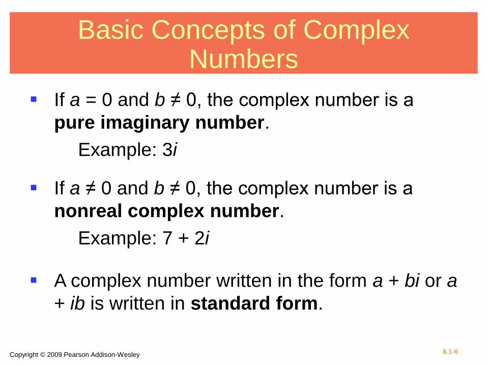
If a = 0 and b ≠ 0, the complex number is a
pure imaginary number.
Example: 3i
If a ≠ 0 and b ≠ 0, the complex number is a
nonreal complex number.
Example: 7 + 2i
A complex number written in the form a + bi or a
+ ib is written in standard form.

Copyright © 2009 Pearson Addison-Wesley 1.1-78.1-7
The Expression

Copyright © 2009 Pearson Addison-Wesley 1.1-88.1-8
Example 1 WRITING AS
Write as the product of real number and i, using the
definition of

Copyright © 2009 Pearson Addison-Wesley 1.1-98.1-9
Example 2 SOLVING QUADRATIC EQUATIONS FOR
COMPLEX SOLUTIONS
Solve each equation.
Solution set:
Solution set:

Copyright © 2009 Pearson Addison-Wesley 1.1-108.1-10
Example 3 SOLVING QUADRATIC EQUATIONS FOR
COMPLEX SOLUTIONS
Write the equation in standard form,
then solve using the quadratic formula with a = 9,
b = –6, and c = 5.

Copyright © 2009 Pearson Addison-Wesley 1.1-118.1-11
Caution
When working with negative radicands,
use the definition before
using any of the other rules for radicals.
In particular, the rule is
valid only when c and d are not both
negative.
For example ,
while ,
so

Copyright © 2009 Pearson Addison-Wesley 1.1-128.1-12
Example 4 FINDING PRODUCTS AND QUOTIENTS
INVOLVING NEGATIVE RADICANDS
Multiply or divide as indicated. Simplify each answer.
Copyright © 2009 Pearson Addison-Wesley 1.1-138.1-13
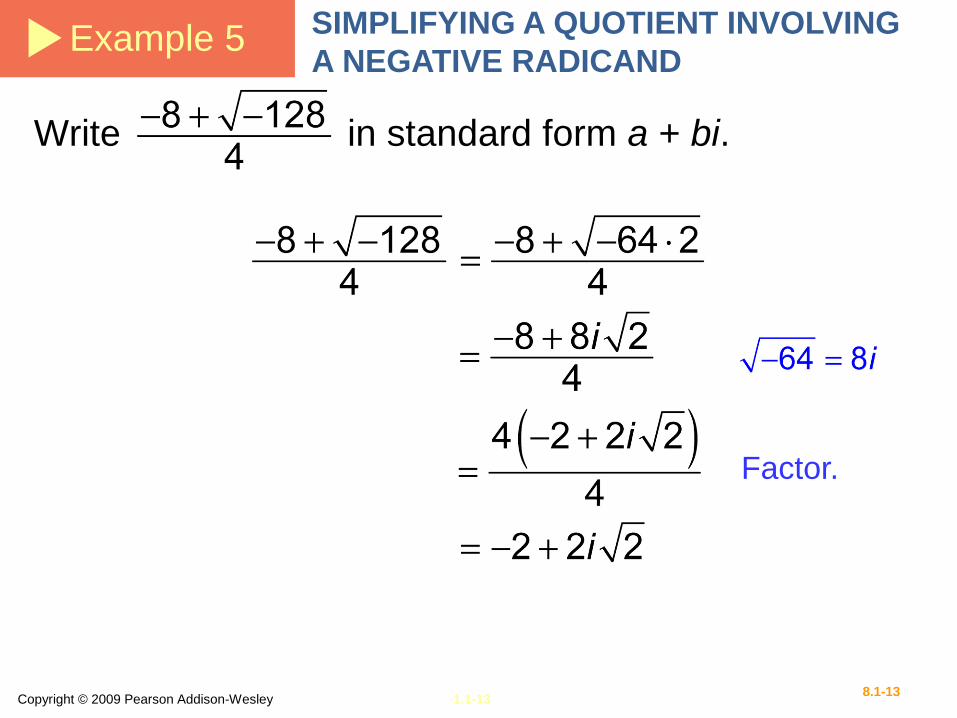
Example 5 SIMPLIFYING A QUOTIENT INVOLVING
A NEGATIVE RADICAND
Write in standard form a + bi.
Factor.

Copyright © 2009 Pearson Addison-Wesley 1.1-148.1-14
Addition and Subtraction of
Complex Numbers
For complex numbers a + bi and c + di,

Copyright © 2009 Pearson Addison-Wesley 1.1-158.1-15
Example 6 ADDING AND SUBTRACTING COMPLEX
NUMBERS
Find each sum or difference.
(a) (3 – 4i) + (–2 + 6i)
= 1 + 2i
= [3 + (–2)] + (–4i + 6i)
(b) (–9 + 7i) + (3 – 15i) = –6 – 8i
(c) (–4 + 3i) – (6 – 7i)
= –10 + 10i
(d) (12 – 5i) – (8 – 3i) + (–4 + 2i)
= 0 + 0i = 0
= (–4 – 6) + [3 – (–7)]i
= (12 – 8 – 4) + (–5 +3 + 2)i

Copyright © 2009 Pearson Addison-Wesley 8.1-16
Multiplication of Complex Numbers

Copyright © 2009 Pearson Addison-Wesley 1.1-178.1-17
Example 7 MULTIPLYING COMPLEX NUMBERS
Find each product.
(a) (2 – 3i)(3 + 4i)
(b) (4 + 3i)2
= 2(3) + (2)(4i) + (–3i)(3) + (–3i)(4i)
= 6 + 8i – 9i – 12i2
= 6 –i – 12(–1)
= 18 – i
= 42 + 2(4)(3i) + (3i)2
= 16 + 24i + 9i2
= 16 + 24i + 9(–1)
= 7 + 24i

Copyright © 2009 Pearson Addison-Wesley 1.1-188.1-18
Example 7 MULTIPLYING COMPLEX NUMBERS
(d) (6 + 5i)(6 – 5i) = 62 – (5i)2
= 36 – 25i2
= 36 – 25(–1)
= 36 + 25
= 61 or 61 + 0i
(c) (2 + i)(–2 – i) = –4 – 2i – 2i – i2
= –4 – 4i – (–1)
= –4 – 4i + 1
= –3 – 4i

Copyright © 2009 Pearson Addison-Wesley 1.1-198.1-19
Example 7 MULTIPLYING COMPLEX NUMBERS
(cont.)
This screen shows how the TI–83/84 Plus displays
the results found in parts (a), (b), and (d) in this
example.

Copyright © 2009 Pearson Addison-Wesley 1.1-208.1-20
Example 8 SIMPLIFYING POWERS OF i
Simplify each power of i.
(a) (b) (c)
Write the given power as a product involving
or .
(a)
(b)
(c)

Copyright © 2009 Pearson Addison-Wesley 1.1-218.1-21
Powers of i
i1 = i i5 = i i9 = i
i2 = 1 i6 = 1 i10 = 1
i3 = i i7 = i i11 = i
i4 = 1 i8 = 1i12 = 1, and so on.

Copyright © 2009 Pearson Addison-Wesley 1.1-228.1-22
Property of Complex Conjugates
For real numbers a and b,

Copyright © 2009 Pearson Addison-Wesley 1.1-238.1-23
Example 9(a) DIVIDING COMPLEX NUMBERS
Write the quotient in standard form a + bi.
Multiply the numerator and denominator by the complex conjugate of the denominator.
i2 = –1
Lowest terms; standard form
Multiply.
Factor.

Copyright © 2009 Pearson Addison-Wesley 1.1-248.1-24
Example 9(b) DIVIDING COMPLEX NUMBERS
Write the quotient in standard form a + bi.
Multiply the numerator and denominator by the complex conjugate of the denominator.
i2 = –1
Standard form
Multiply.
This screen shows how
the TI–83/84 Plus
displays the results in
this example.

Copyright © 2009 Pearson Addison-Wesley 8.2-1
8Complex Numbers, Polar Equations, and Parametric Equations

Copyright © 2009 Pearson Addison-Wesley 8.2-2
8.1 Complex Numbers
8.2 Trigonometric (Polar) Form of Complex Numbers
8.3 The Product and Quotient Theorems
8.4 De Moivre’s Theorem; Powers and Roots of Complex Numbers
8.5 Polar Equations and Graphs
8.6 Parametric Equations, Graphs, and Applications
8Complex Numbers, Polar Equations, and Parametric Equations

Copyright © 2009 Pearson Addison-Wesley 1.1-38.2-3
Trigonometric (Polar) Form
of Complex Numbers8.2
The Complex Plane and Vector Representation ▪ Trigonometric (Polar) Form ▪ Converting Between Rectangular and Trigonometric (Polar) Forms ▪ An Application of Complex Numbers to Fractals

Copyright © 2009 Pearson Addison-Wesley 8.2-4
The Complex Plane and Vector Representation
Horizontal axis: real axis
Vertical axis: imaginary axis
Each complex number a + bi
determines a unique position
vector with initial point (0, 0)
and terminal point (a, b).

Copyright © 2009 Pearson Addison-Wesley 8.2-5
The Complex Plane and Vector Representation
The sum of two complex numbers is represented
by the vector that is the resultant of the vectors
corresponding to the two numbers.
(4 + i) + (1 + 3i) = 5 + 4i

Copyright © 2009 Pearson Addison-Wesley 1.1-68.2-6
Example 1 EXPRESSING THE SUM OF COMPLEX
NUMBERS GRAPHICALLY
Find the sum of 6 – 2i and –4 – 3i. Graph both
complex numbers and their resultant.
(6 – 2i) + (–4 – 3i) = 2 – 5i

Copyright © 2009 Pearson Addison-Wesley 1.1-78.2-7
Relationships Among x, y, r, and θ.

Copyright © 2009 Pearson Addison-Wesley 1.1-88.2-8
Trigonometric (Polar) Form
of a Complex Number
The expression r(cos θ + i sin θ) is called
the trigonometric form (or polar form) of
the complex number x + yi.
The expression cos θ + i sin θ is
sometimes abbreviated cis θ.
Using this notation, r(cos θ + i sin θ) is
written r cis θ.
The number r is the absolute value (or modulus)
of x + yi, and θ is the argument of x + yi.

Copyright © 2009 Pearson Addison-Wesley 1.1-98.2-9
Example 2 CONVERTING FROM TRIGONOMETRIC
FORM TO RECTANGULAR FORM
Express 2(cos 300° + i sin 300°) in rectangular form.
The graphing calculator
screen confirms the
algebraic solution. The
imaginary part is an
approximation for

Copyright © 2009 Pearson Addison-Wesley 1.1-108.2-10
Converting From Rectangular Form to
Trigonometric Form
Step 1 Sketch a graph of the number x + yi in the complex plane.
Step 2 Find r by using the equation
Step 3 Find θ by using the equation
choosing the quadrant indicated in Step 1.
Copyright © 2009 Pearson Addison-Wesley 1.1-118.2-11
Caution
Be sure to choose the correct
quadrant for θ by referring to the
graph sketched in Step 1.

Copyright © 2009 Pearson Addison-Wesley 1.1-128.2-12
Example 3(a) CONVERTING FROM RECTANGULAR
FORM TO TRIGONOMETRIC FORM
Write in trigonometric form. (Use radian
measure.)
Sketch the graph of
in the complex plane.
Step 1:
Step 2:

Copyright © 2009 Pearson Addison-Wesley 1.1-138.2-13
Example 3(a) CONVERTING FROM RECTANGULAR
FORM TO TRIGONOMETRIC FORM
(continued)
Step 3:
The reference angle for θ is
The graph shows that θ is in
quadrant II, so θ =

Copyright © 2009 Pearson Addison-Wesley 1.1-148.2-14
Example 3(b) CONVERTING FROM RECTANGULAR
FORM TO TRIGONOMETRIC FORM
Write –3i in trigonometric form. (Use degree measure.)
Sketch the graph of –3i in
the complex plane.
We cannot find θ by using
because x = 0.
From the graph, a value for θ is 270 .

Copyright © 2009 Pearson Addison-Wesley 1.1-158.2-15
Example 4 CONVERTING BETWEEN
TRIGONOMETRIC AND RECTANGULAR
FORMS USING CALCULATOR
APPROXIMATIONS
Write each complex number in its alternative form,
using calculator approximations as necessary.
(a) 6(cos 115 + i sin 115 ) ≈ –2.5357 + 5.4378i

Copyright © 2009 Pearson Addison-Wesley 1.1-168.2-16
Example 4 CONVERTING BETWEEN
TRIGONOMETRIC AND RECTANGULAR
FORMS USING CALCULATOR
APPROXIMATIONS (continued)
(b) 5 – 4i
A sketch of 5 – 4i shows that θ
must be in quadrant IV.
The reference angle for θ is approximately –38.66 .
The graph shows that θ is in quadrant IV, so
θ = 360 – 38.66 = 321.34 .

Copyright © 2009 Pearson Addison-Wesley 1.1-178.2-17
Example 5 DECIDING WHETHER A COMPLEX
NUMBER IS IN THE JULIA SET
The figure shows the fractal called the Julia set.
To determine if a complex number z = a + bi belongs
to the Julia set, repeatedly compute the values of

Copyright © 2009 Pearson Addison-Wesley 1.1-188.2-18
Example 5 DECIDING WHETHER A COMPLEX
NUMBER IS IN THE JULIA SET (cont.)
If the absolute values of any of the resulting complex
numbers exceed 2, then the complex number z is not
in the Julia set. Otherwise z is part of this set and the
point (a, b) should be shaded in the graph.

Copyright © 2009 Pearson Addison-Wesley 1.1-198.2-19
Example 5 DECIDING WHETHER A COMPLEX
NUMBER IS IN THE JULIA SET (cont.)
Determine whether each number belongs to the Julia
set.
The calculations
repeat as 0, –1, 0, –1,
and so on.
The absolute values are either 0 or 1, which do not
exceed 2, so 0 + 0i is in the Julia set, and the point
(0, 0) is part of the graph.

Copyright © 2009 Pearson Addison-Wesley 1.1-208.2-20
Example 5 DECIDING WHETHER A COMPLEX
NUMBER IS IN THE JULIA SET (cont.)
The absolute value is
so 1 + 1i is not in the Julia set and (1, 1) is not part of the graph.

Copyright © 2009 Pearson Addison-Wesley 8.3-1
8Complex Numbers, Polar Equations, and Parametric Equations

Copyright © 2009 Pearson Addison-Wesley 8.3-2
8.1 Complex Numbers
8.2 Trigonometric (Polar) Form of Complex Numbers
8.3 The Product and Quotient Theorems
8.4 De Moivre’s Theorem; Powers and Roots of Complex Numbers
8.5 Polar Equations and Graphs
8.6 Parametric Equations, Graphs, and Applications
8Complex Numbers, Polar Equations, and Parametric Equations

Copyright © 2009 Pearson Addison-Wesley 1.1-38.3-3
The Product and Quotient
Theorems8.3
Products of Complex Numbers in Trigonometric Form ▪Quotients of Complex Numbers in Trigonometric Form

Copyright © 2009 Pearson Addison-Wesley 1.1-48.3-4
Product Theorem
are any two complex numbers, then
In compact form, this is written

Copyright © 2009 Pearson Addison-Wesley 1.1-58.3-5
Example 1 USING THE PRODUCT THEOREM
Find the product of 3(cos 45° + i sin 45°) and
2(cos 135° + i sin 135°). Write the result in
rectangular form.

Copyright © 2009 Pearson Addison-Wesley 1.1-68.3-6
Quotient Theorem
are any two complex numbers, where
In compact form, this is written

Copyright © 2009 Pearson Addison-Wesley 1.1-78.3-7
Example 2 USING THE QUOTIENT THEOREM
Find the quotient Write the result in
rectangular form.

Copyright © 2009 Pearson Addison-Wesley 1.1-88.3-8
Example 3 USING THE PRODUCT AND QUOTIENT
THEOREMS WITH A CALCULATOR
Use a calculator to find the following. Write the results
in rectangular form.

Copyright © 2009 Pearson Addison-Wesley 1.1-98.3-9
Example 3 USING THE PRODUCT AND QUOTIENT
THEOREMS WITH A CALCULATOR
(continued)

Copyright © 2009 Pearson Addison-Wesley 8.4-1
8Complex Numbers, Polar Equations, and Parametric Equations

Copyright © 2009 Pearson Addison-Wesley 8.4-2
8.1 Complex Numbers
8.2 Trigonometric (Polar) Form of Complex Numbers
8.3 The Product and Quotient Theorems
8.4 De Moivre’s Theorem; Powers and Roots of Complex Numbers
8.5 Polar Equations and Graphs
8.6 Parametric Equations, Graphs, and Applications
8Complex Numbers, Polar Equations, and Parametric Equations

Copyright © 2009 Pearson Addison-Wesley 1.1-38.4-3
De Moivre’s Theorem; Powers
and Roots of Complex Numbers8.4
Powers of Complex Numbers (De Moivre’s Theorem) ▪ Roots of Complex Numbers

Copyright © 2009 Pearson Addison-Wesley 1.1-48.4-4
De Moivre’s Theorem
is a complex number, then
In compact form, this is written

Copyright © 2009 Pearson Addison-Wesley 1.1-58.4-5
Example 1 FINDING A POWER OF A COMPLEX
NUMBER
Find and express the result in rectangular
form.
First write in trigonometric form.
Because x and y are both positive, θ is in quadrant I,
so θ = 60 .

Copyright © 2009 Pearson Addison-Wesley 1.1-68.4-6
Example 1 FINDING A POWER OF A COMPLEX
NUMBER (continued)
Now apply De Moivre’s theorem.
480 and 120 are coterminal.
Rectangular form

Copyright © 2009 Pearson Addison-Wesley 1.1-78.4-7
nth Root
For a positive integer n, the complex number a + bi is an nth root of the complex number x + yi if

Copyright © 2009 Pearson Addison-Wesley 1.1-88.4-8
nth Root Theorem
If n is any positive integer, r is a positive real number, and θ is in degrees, then the nonzero complex number r(cos θ + i sin θ) has exactly n distinct nth roots, given by
where

Copyright © 2009 Pearson Addison-Wesley 1.1-98.4-9
Note
In the statement of the nth root theorem,
if θ is in radians, then

Copyright © 2009 Pearson Addison-Wesley 1.1-108.4-10
Example 2 FINDING COMPLEX ROOTS
Find the two square roots of 4i. Write the roots in
rectangular form.
Write 4i in trigonometric form:
The square roots have absolute value
and argument

Copyright © 2009 Pearson Addison-Wesley 1.1-118.4-11
Example 2 FINDING COMPLEX ROOTS (continued)
Since there are two square roots, let k = 0 and 1.
Using these values for , the square roots are

Copyright © 2009 Pearson Addison-Wesley 1.1-128.4-12
Example 2 FINDING COMPLEX ROOTS (continued)

Copyright © 2009 Pearson Addison-Wesley 1.1-138.4-13
Example 3 FINDING COMPLEX ROOTS
Find all fourth roots of Write the roots in
rectangular form.
Write in trigonometric form:
The fourth roots have absolute value
and argument

Copyright © 2009 Pearson Addison-Wesley 1.1-148.4-14
Example 3 FINDING COMPLEX ROOTS (continued)
Since there are four roots, let k = 0, 1, 2, and 3.
Using these values for α, the fourth roots are
2 cis 30 , 2 cis 120 , 2 cis 210 , and 2 cis 300 .

Copyright © 2009 Pearson Addison-Wesley 1.1-158.4-15
Example 3 FINDING COMPLEX ROOTS (continued)

Copyright © 2009 Pearson Addison-Wesley 1.1-168.4-16
Example 3 FINDING COMPLEX ROOTS (continued)
The graphs of the roots lie on a circle with center at the origin and radius 2. The roots are equally spaced about the circle, 90 apart.

Copyright © 2009 Pearson Addison-Wesley 1.1-178.4-17
Example 4 SOLVING AN EQUATION BY FINDING
COMPLEX ROOTS
Find all complex number solutions of x5 – i = 0. Graph
them as vectors in the complex plane.
There is one real solution, 1, while there are five
complex solutions.
Write 1 in trigonometric form:

Copyright © 2009 Pearson Addison-Wesley 1.1-188.4-18
Example 4 SOLVING AN EQUATION BY FINDING
COMPLEX ROOTS (continued)
The fifth roots have absolute value and
argument
Since there are five roots, let k = 0, 1, 2, 3, and 4.
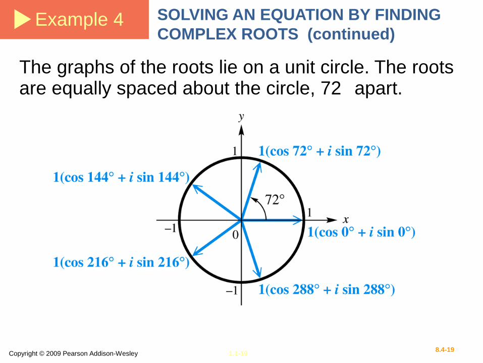
Solution set: {cis 0 , cis 72 , cis 144 , cis 216 , cis 288 }
Copyright © 2009 Pearson Addison-Wesley 1.1-198.4-19
Example 4 SOLVING AN EQUATION BY FINDING
COMPLEX ROOTS (continued)
The graphs of the roots lie on a unit circle. The roots are equally spaced about the circle, 72 apart.
Copyright © 2009 Pearson Addison-Wesley 8.5-1
8Complex Numbers, Polar Equations, and Parametric Equations

Copyright © 2009 Pearson Addison-Wesley 8.5-2
8.1 Complex Numbers
8.2 Trigonometric (Polar) Form of Complex Numbers
8.3 The Product and Quotient Theorems
8.4 De Moivre’s Theorem; Powers and Roots of Complex Numbers
8.5 Polar Equations and Graphs
8.6 Parametric Equations, Graphs, and Applications
8Complex Numbers, Polar Equations, and Parametric Equations

Copyright © 2009 Pearson Addison-Wesley 1.1-38.5-3
Polar Equations and Graphs8.5Polar Coordinate System ▪ Graphs of Polar Equations ▪Converting from Polar to Rectangular Equations ▪ Classifying Polar Equations

Copyright © 2009 Pearson Addison-Wesley 8.5-4
Polar Coordinate System
The polar coordinate system is based on a point,
called the pole, and a ray, called the polar axis.

Copyright © 2009 Pearson Addison-Wesley 8.5-5
Polar Coordinate System
Point P has rectangular
coordinates (x, y).
Point P can also be located by
giving the directed angle θ from
the positive x-axis to ray OP
and the directed distance r
from the pole to point P.
The polar coordinates of point
P are (r, θ).
Copyright © 2009 Pearson Addison-Wesley 8.5-6
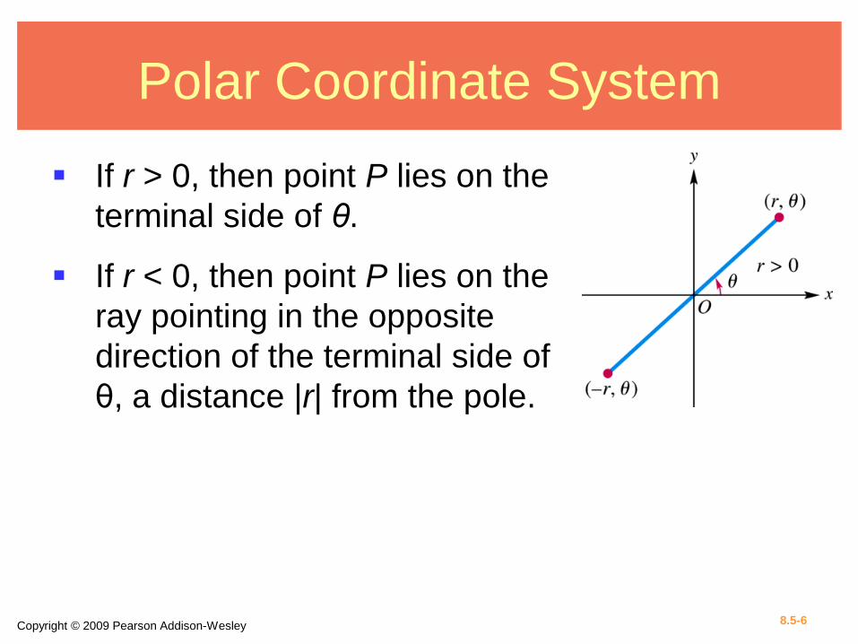
Polar Coordinate System
If r > 0, then point P lies on the
terminal side of θ.
If r < 0, then point P lies on the
ray pointing in the opposite
direction of the terminal side of
θ, a distance |r| from the pole.

Copyright © 2009 Pearson Addison-Wesley 1.1-78.5-7
Rectangular and Polar Coordinates
If a point has rectangular coordinates (x, y) and polar coordinates (r, ), then these coordinates are related as follows.

Copyright © 2009 Pearson Addison-Wesley 1.1-88.5-8
Example 1 PLOTTING POINTS WITH POLAR
COORDINATES
Plot each point by hand in the polar coordinate
system. Then, determine the rectangular coordinates
of each point.
(a) P(2, 30 )
r = 2 and θ = 30 , so
point P is located 2 units
from the origin in the
positive direction making
a 30 angle with the
polar axis.

Copyright © 2009 Pearson Addison-Wesley 1.1-98.5-9
Example 1 PLOTTING POINTS WITH POLAR
COORDINATES (continued)
Using the conversion formulas:
The rectangular coordinates are

Copyright © 2009 Pearson Addison-Wesley 1.1-108.5-10
Example 1 PLOTTING POINTS WITH POLAR
COORDINATES (continued)
Since r is negative, Q is 4
units in the opposite
direction from the pole on an
extension of the ray.
The rectangular coordinates are
Copyright © 2009 Pearson Addison-Wesley 1.1-118.5-11
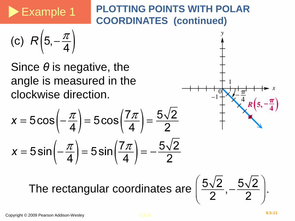
Example 1 PLOTTING POINTS WITH POLAR
COORDINATES (continued)
Since θ is negative, the
angle is measured in the
clockwise direction.
The rectangular coordinates are

Copyright © 2009 Pearson Addison-Wesley 1.1-128.5-12
Note
While a given point in the plane can
have only one pair of rectangular
coordinates, this same point can
have an infinite number of pairs of
polar coordinates.

Copyright © 2009 Pearson Addison-Wesley 1.1-138.5-13
Example 2 GIVING ALTERNATIVE FORMS FOR
COORDINATES OF A POINT
(a) Give three other pairs of polar coordinates for the
point P(3, 140 ).
Three pairs of polar coordinates for the point
P(3, 140 ) are (3, –220 ), (−3, 320 ), and (−3, −40 ).

Copyright © 2009 Pearson Addison-Wesley 1.1-148.5-14
Example 2 GIVING ALTERNATIVE FORMS FOR
COORDINATES OF A POINT (continued)
(b) Determine two pairs of polar coordinates for the
point with the rectangular coordinates (–1, 1).
The point (–1, 1) lies in quadrant II.
Since one possible value for θ is 135 .
Two pairs of polar coordinates are

Copyright © 2009 Pearson Addison-Wesley 8.5-15
Graphs of Polar Equations
An equation in which r and θ are the variables is a
polar equation.
Derive the polar equation of the line ax + by = c as
follows:
General form for the polar equation of a line
Convert from rectangular to polar coordinates.
Factor out r.

Copyright © 2009 Pearson Addison-Wesley 8.5-16
Graphs of Polar Equations
Derive the polar equation of the circle x2 + y2 = a2 as
follows:
General form for the polar equation of a circle

Copyright © 2009 Pearson Addison-Wesley 1.1-178.5-17
Example 3 EXAMINING POLAR AND
RECTANGULAR EQUATION OF LINES
AND CIRCLES
For each rectangular equation, give the equivalent
polar equation and sketch its graph.
(a) y = x – 3
In standard form, the equation is x – y = 3, so a = 1,
b = –1, and c = 3.
The general form for the polar equation of a line is
y = x – 3 is equivalent to

Copyright © 2009 Pearson Addison-Wesley 1.1-188.5-18
Example 3 EXAMINING POLAR AND
RECTANGULAR EQUATION OF LINES
AND CIRCLES (continued)

Copyright © 2009 Pearson Addison-Wesley 1.1-198.5-19
Example 3 EXAMINING POLAR AND
RECTANGULAR EQUATION OF LINES
AND CIRCLES (continued)
(b)
This is the graph of a circle with center at the origin
and radius 2.
Note that in polar coordinates it is possible for r < 0.

Copyright © 2009 Pearson Addison-Wesley 1.1-208.5-20
Example 3 EXAMINING POLAR AND
RECTANGULAR EQUATION OF LINES
AND CIRCLES (continued)

Copyright © 2009 Pearson Addison-Wesley 1.1-218.5-21
Example 4 GRAPHING A POLAR EQUATION
(CARDIOID)
Find some ordered pairs to determine a pattern of
values of r.

Copyright © 2009 Pearson Addison-Wesley 1.1-228.5-22
Example 4 GRAPHING A POLAR EQUATION
(CARDIOID)
Connect the points in order from (2, 0 ) to (1.9, 30 )
to (1.7, 48 ) and so on.

Copyright © 2009 Pearson Addison-Wesley 1.1-238.5-23
Example 4 GRAPHING A POLAR EQUATION
(CARDIOD) (continued)
Choose degree mode and graph values of θ in the
interval [0 , 360 ].

Copyright © 2009 Pearson Addison-Wesley 1.1-248.5-24
Example 5 GRAPHING A POLAR EQUATION
(ROSE)
Find some ordered pairs to determine a pattern of
values of r.

Copyright © 2009 Pearson Addison-Wesley 1.1-258.5-25
Example 5 GRAPHING A POLAR EQUATION
(ROSE) (continued)
Connect the points in order from (3, 0 ) to (2.6, 15 )
to (1.5, 30 ) and so on. Notice how the graph is
developed with a continuous curve, starting with the
upper half of the right horizontal leaf and ending with
the lower half of that leaf.
Copyright © 2009 Pearson Addison-Wesley 1.1-268.5-26
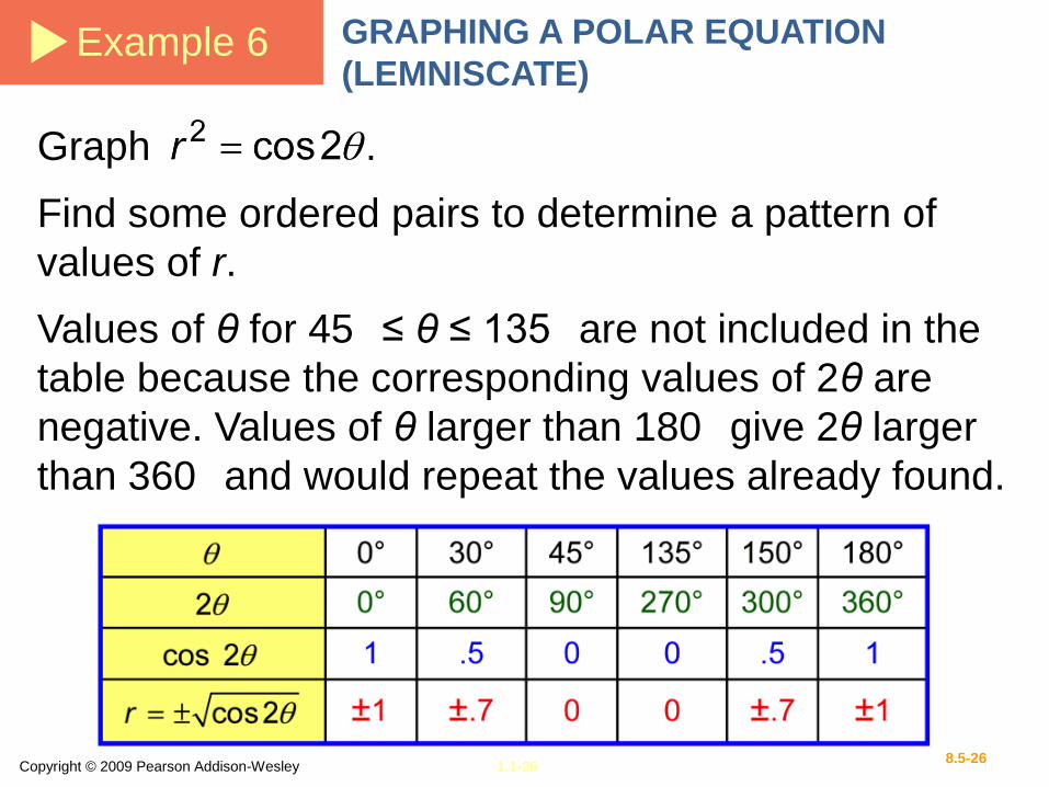
Example 6 GRAPHING A POLAR EQUATION
(LEMNISCATE)
Find some ordered pairs to determine a pattern of
values of r.
Graph .
Values of θ for 45 ≤ θ ≤ 135 are not included in the
table because the corresponding values of 2θ are
negative. Values of θ larger than 180 give 2θ larger
than 360 and would repeat the values already found.

Copyright © 2009 Pearson Addison-Wesley 1.1-278.5-27
Example 6 GRAPHING A POLAR EQUATION
(LEMNISCATE) (continued)

Copyright © 2009 Pearson Addison-Wesley 1.1-288.5-28
Example 6 GRAPHING A POLAR EQUATION
(LEMNISCATE) (continued)
To graph with a graphing calculator, let

Copyright © 2009 Pearson Addison-Wesley 1.1-298.5-29
Example 7 GRAPHING A POLAR EQUATION
(SPIRAL OF ARCHIMEDES)
Find some ordered pairs to determine a pattern of
values of r.
Since r = 2θ, also consider negative values of θ.
Graph r = 2θ, (θ measured in radians).

Copyright © 2009 Pearson Addison-Wesley 1.1-308.5-30
Example 7 GRAPHING A POLAR EQUATION
(SPIRAL OF ARCHIMEDES) (continued)

Copyright © 2009 Pearson Addison-Wesley 1.1-318.5-31
Example 8 CONVERTING A POLAR EQUATION TO
A RECTANGULAR EQUATION
Convert the equation to rectangular
coordinates and graph.
Multiply both sides by 1 + sin θ.
Square both sides.
Expand.
Rectangular form

Copyright © 2009 Pearson Addison-Wesley 1.1-328.5-32
Example 8 CONVERTING A POLAR EQUATION TO
A RECTANGULAR EQUATION (cont.)
The graph is plotted with the calculator in polar mode.

Copyright © 2009 Pearson Addison-Wesley 8.5-33
Classifying Polar Equations
Circles and Lemniscates

Copyright © 2009 Pearson Addison-Wesley 8.5-34
Classifying Polar Equations
Limaçons

Copyright © 2009 Pearson Addison-Wesley 8.5-35
Classifying Polar Equations
Rose Curves
2n leaves if n is even,
n ≥ 2
n leaves if n is odd

Copyright © 2009 Pearson Addison-Wesley 8.6-1
8Complex Numbers, Polar Equations, and Parametric Equations

Copyright © 2009 Pearson Addison-Wesley 8.6-2
8.1 Complex Numbers
8.2 Trigonometric (Polar) Form of Complex Numbers
8.3 The Product and Quotient Theorems
8.4 De Moivre’s Theorem; Powers and Roots of Complex Numbers
8.5 Polar Equations and Graphs
8.6 Parametric Equations, Graphs, and Applications
8Complex Numbers, Polar Equations, and Parametric Equations

Copyright © 2009 Pearson Addison-Wesley 1.1-38.6-3
Parametric Equations, Graphs,
and Applications8.6
Basic Concepts ▪ Parametric Graphs and Their Rectangular Equivalents ▪ The Cycloid ▪ Applications of Parametric Equations

Copyright © 2009 Pearson Addison-Wesley 1.1-48.6-4
Parametric Equations of a Plane Curve
A plane curve is a set of points (x, y) such that x = f(t), y = g(t), and f and g are both defined on an interval I.
The equations x = f(t) and y = g(t) are
parametric equations with parameter t.

Copyright © 2009 Pearson Addison-Wesley 1.1-58.6-5
Example 1 GRAPHING A PLANE CURVE DEFINED
PARAMETRICALLY
Let x = t2 and y = 2t + 3 for t in [–3, 3]. Graph the set
of ordered pairs (x, y).
Make a table of
corresponding values
of t, x, and y over the
domain of t. Then plot
the points.

Copyright © 2009 Pearson Addison-Wesley 1.1-68.6-6
Example 1 GRAPHING A PLANE CURVE DEFINED
PARAMETRICALLY (continued)
The arrowheads indicate the direction the curve
traces as t increases.

Copyright © 2009 Pearson Addison-Wesley 1.1-78.6-7
Example 1 GRAPHING A PLANE CURVE DEFINED
PARAMETRICALLY (continued)

Copyright © 2009 Pearson Addison-Wesley 1.1-88.6-8
Example 2 FINDING AN EQUIVALENT
RECTANGULAR EQUATION
Find a rectangular equation for the plane curve
defined as x = t2 and y = 2t + 3 for t in [–3, 3].
(Example 1)
To eliminate the parameter t, solve either equation for t.
Since y = 2t + 3 leads to a unique solution for t, choose
that equation.
The rectangular equation is , for x in [0, 9].
Copyright © 2009 Pearson Addison-Wesley 1.1-98.6-9
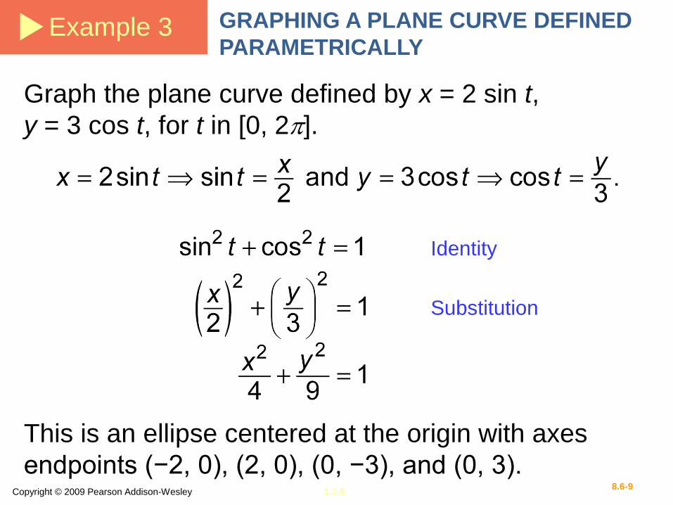
Example 3 GRAPHING A PLANE CURVE DEFINED
PARAMETRICALLY
Graph the plane curve defined by x = 2 sin t,
y = 3 cos t, for t in [0, 2].
Identity
Substitution
This is an ellipse centered at the origin with axes
endpoints (−2, 0), (2, 0), (0, −3), and (0, 3).

Copyright © 2009 Pearson Addison-Wesley 1.1-108.6-10
Example 3 GRAPHING A PLANE CURVE DEFINED
PARAMETRICALLY (continued)

Copyright © 2009 Pearson Addison-Wesley 1.1-118.6-11
Note
Parametric representations of a curve
are not unique.
In fact, there are infinitely many
parametric representations of a given
curve.

Copyright © 2009 Pearson Addison-Wesley 1.1-128.6-12
Example 4 FINDING ALTERNATIVE PARAMETRIC
EQUATION FORMS
Give two parametric representations for the equation
of the parabola
The simplest choice is
Another choice is
Sometimes trigonometric functions are desirable.
One choice is

Copyright © 2009 Pearson Addison-Wesley 8.6-13
The Cycloid
The path traced by a fixed point on the circumference
of a circle rolling along a line is called a cycloid.
A cycloid is defined by

Copyright © 2009 Pearson Addison-Wesley 8.6-14
The Cycloid
If a flexible cord or wire goes through points P and Q,
and a bead is allowed to slide due to the force of
gravity without friction along this path from P to Q, the
path that requires the shortest time takes the shape of
an inverted cycloid.
Copyright © 2009 Pearson Addison-Wesley 1.1-158.6-15
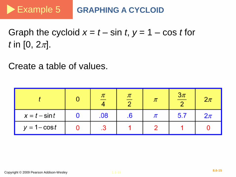
Example 5 GRAPHING A CYCLOID
Graph the cycloid x = t – sin t, y = 1 – cos t for
t in [0, 2].
Create a table of values.

Copyright © 2009 Pearson Addison-Wesley 1.1-168.6-16
Example 5 GRAPHING A CYCLOID (continued)
Plotting the ordered pairs (x, y) from the table of
values leads to the portion of the graph for t in [0, 2].

Copyright © 2009 Pearson Addison-Wesley 8.6-17
Applications of Parametric Equations
If a ball is thrown with a velocity of v feet per second
at an angle θ with the horizontal, its flight can be
modeled by the parametric equations
where t is in seconds, and h is the ball’s initial height
in feet above the ground.

Copyright © 2009 Pearson Addison-Wesley 1.1-188.6-18
Example 6 SIMULATING MOTION WITH
PARAMETRIC EQUATIONS
Three golf balls are hit simultaneously into the air at
132 feet per second (90 mph) at angles of 30°, 50°,
and 70° with the horizontal.
(a) Assuming the ground is level, determine graphically
which ball travels the farthest. Estimate this distance.
The three sets of parametric equations determined by
the three golf balls (h = 0) are

Copyright © 2009 Pearson Addison-Wesley 1.1-198.6-19
Example 6 SIMULATING MOTION WITH
PARAMETRIC EQUATIONS (continued)
Graph the three sets of parametric equations using a
graphing calculator.
Using the TRACE feature, we find that the ball that
travels the farthest is the ball hit at 50 . It travels about
540 ft.

Copyright © 2009 Pearson Addison-Wesley 1.1-208.6-20
Example 6 SIMULATING MOTION WITH
PARAMETRIC EQUATIONS (continued)
(b) Which ball reaches the greatest height? Estimate
this height.
Using the TRACE feature, we find that the ball that
reaches the greatest height is the ball hit at 70 . It
reaches about 240 ft.

Copyright © 2009 Pearson Addison-Wesley 1.1-218.6-21
Example 7 EXAMINING PARAMETRIC EQUATIONS
OF FLIGHT
Jack launches a small rocket from a table that is 3.36 ft
above the ground. Its initial velocity is 64 ft per sec,
and it is launched at an angle of 30 with respect to the
ground. Find the rectangular equation that models its
path. What type of path does the rocket follow?
The path of the rocket is defined by
or equivalently,

Copyright © 2009 Pearson Addison-Wesley 1.1-228.6-22
Example 7 EXAMINING PARAMETRIC EQUATIONS
OF FLIGHT (continued)
Substituting into the other parametric equation yields
Because this equation defines a parabola, the rocket
follows a parabolic path.

Copyright © 2009 Pearson Addison-Wesley 1.1-238.6-23
Example 8 ANALYZING THE PATH OF A
PROJECTILE
Determine the total flight time and the horizontal
distance traveled by the rocket in Example 7.
From Example 7 (slide 21), we have
which tells the vertical position of the rocket at time t.
To determine when the rocket hits the ground, solve

Copyright © 2009 Pearson Addison-Wesley 1.1-248.6-24
Example 8 ANALYZING THE PATH OF A
PROJECTILE (continued)
The flight time is about 2.1 seconds.

Copyright © 2009 Pearson Addison-Wesley 1.1-258.6-25
Example 8 ANALYZING THE PATH OF A
PROJECTILE (continued)
The rocket has traveled about 116.4 feet.
Substitute 2.1 for t into the parametric equation that
models the horizontal position,
The solution can be verified
by graphing and
and using the TRACE feature.


![Contents arXiv:1408.3992v1 [math.GT] 18 Aug 2014users.monash.edu/~normd/documents/Do-Dyer-Mathews-14.pdfnumbers to intersection numbers on Mg,n as well as to derive string and dilaton](https://img.dokumen.tips/doc/110x75/60c09b8277ed1b1cfb33fe85/contents-arxiv14083992v1-mathgt-18-aug-normddocumentsdo-dyer-mathews-14pdf.jpg)


