Complex Fan Analysis, an Extension of ACT-R Fan Effect Model

by

Kam-Hung Kwok

B.Eng., M.Sc.

A thesis submitted to the Faculty of Graduate and Postdoctoral Affairs in partial fulfillment of the requirements for the degree of

Doctor of Philosophy

in

Cognitive Science

Carleton University

Ottawa, Ontario

© 2015, Kam-Hung Kwok

ii

Abstract

The purpose of this study was to determine whether Anderson’s ACT-R fan

model could account for the fan effect under more complex conditions. Specifically,

overlapping datasets were used so that related facts learned in one experiment could

potentially affect the fan in other experiments. The study of the overlapping datasets

made it possible to study an inference task by combining facts learned in separate

experiments. Four experiments with human subjects were carried out and human

performance was compared to predictions from Anderson’s ACT-R fan model. The

results showed ACT-R fan model could be used as a basic building block for explaining

complex fan tasks (some high-level cognitive tasks); ACT-R fan model with no

adjustments to the parameters provided a reasonable account for human performance

across all of the experiments. The results suggest that recently learned related facts have

an effect on the fan (Experiment 2). But, it was found that the related facts learned ten

months earlier showed no interference due to fan but there was a main learning effect

which affected reaction times (Experiment 4).

In terms of relational inferences from overlapping datasets, the results indicated a

dual retrieval process with additional search process is more consistent with Anderson’s

fan model than with Radvansky’s mental models approach or a parallel retrieval

approach. Both Radvansky’s mental models approach and a parallel retrieval approach

predicted a single retrieval process (Experiment 3).

This study also evaluated an alternative way of implementing fan models using a

holographic memory system. The four complex fan experiment results were compared to

predictions from an ACT-R simulation of the fan and predictions using the Holographic

Declarative Memory (HDM) module in Python ACT-R, a version of ACT-R (Experiment

5). Although HDM is based on a different representation, it is conceptually related to

ACT-R‟s fan model in that both can be understood as using prior probabilities as

iii

activation for memory retrieval. The results showed all the fan models continue to

provide a reasonable account for the human results indicating that the power of the fan

model comes from the conceptual structure of the theory and not the specific ways in

which it is implemented. All of the models have some deviations from the human data

suggesting that all of the models are close descriptions but none is perfect.

iv

Acknowledgements

Soli Deo Gloria. Many thanks to Robert West, Jo-Anne Lefevre who have been a

constant source of help; to my family, Season, Ada, Peter, Nancy, Nick, Dixie, Swan,

Lydia, Francis, Nathan, Leah and Alex for their unwavering support; to Dale, Roger, HF

Lee, Don, Lucette, and Johann, who are my faithful friends and sounding-boards; to

innumerable faculty members and friends at the Cognitive Institute who have inspired

me.

v

Table of Contents

Abstract .............................................................................................................................. ii

Acknowledgements .......................................................................................................... iv

Table of Contents .............................................................................................................. v

List of Tables .................................................................................................................. viii

List of Figures ................................................................................................................... ix

List of Appendices ........................................................................................................... xii

Introduction ........................................................................................................... 14 1 Chapter:

1.1 Cognitive Architecture ............................................................................................. 14

1.2 ACT-R General Description .................................................................................... 14

1.3 Spreading Activation ................................................................................................ 19

1.4 ACT-R Memory Modeling ...................................................................................... 20

1.5 Dissertation Overview .............................................................................................. 22

Fan Effect, ACT-R Fan Analysis and Fan Paradigm ............................................ 27 2 Chapter:

2.1 Fan Effect ................................................................................................................. 27

2.2 ACT-R Fan Model and Analysis .............................................................................. 33

2.3 The Emergence of a Fan Effect Paradigm ............................................................... 42

Complex Fan Paradigm ........................................................................................ 43 3 Chapter:

3.1 Complex Fan Experiment Design ............................................................................ 45

3.2 Complex Fan Experiments for Relational Inference ................................................ 46

Experiment 1: Object-Container Experiment ....................................................... 48 4 Chapter:

4.1 Method ..................................................................................................................... 48

4.2 Models construction ................................................................................................. 51

4.3 Results ...................................................................................................................... 52

4.4 Discussion ................................................................................................................ 58

vi

4.5 Conclusion ............................................................................................................... 59

Experiment 2: Container-Location Experiment .................................................... 61 5 Chapter:

5.1 Method ..................................................................................................................... 61

5.2 Models construction ................................................................................................. 63

5.3 Results ...................................................................................................................... 64

5.4 Discussion ................................................................................................................ 77

5.5 Conclusion ............................................................................................................... 80

Experiment 3 – Object-Location (inference test) .................................................. 81 6 Chapter:

6.1 Method ..................................................................................................................... 81

6.2 Model Construction: ACT-R model for complex fan .............................................. 83

6.3 Results ...................................................................................................................... 86

6.4 Discussion ................................................................................................................ 94

6.5 Conclusion ............................................................................................................... 95

Experiment 4 - a follow-up experiment on dataset boundary ............................... 97 7 Chapter:

7.1 Method ..................................................................................................................... 98

7.2 Model Construction ................................................................................................ 100

7.3 Results .................................................................................................................... 102

7.4 Discussion .............................................................................................................. 115

7.5 Conclusion ............................................................................................................. 118

Experiment 5: Holographic Declarative Memory for Complex Fan .................. 120 8 Chapter:

8.1 Holographic declarative memory module background .......................................... 121

8.2 Model construction for fan and complex fan with HDM ....................................... 122

8.3 HDM simulation and human performance comparisons ........................................ 123

8.4 Experiment 1 and HDM Results ............................................................................ 123

8.5 Experiment 2 and HDM Results ............................................................................ 125

8.6 Experiment 3 and HDM results .............................................................................. 128

vii

8.7 Experiment 4 and HDM Results ............................................................................ 130

8.8 Conclusions ............................................................................................................ 132

Conclusions and Summary ................................................................................. 134 9 Chapter:

Appendices ..................................................................................................................... 137

Bibliography and References ....................................................................................... 306

viii

List of Tables

Table 1 Average Reaction Times (latencies) in seconds as a function of fan

(Anderson and Reder, 1999) ····································································· 34

Table 2 ACT-R Reaction Time Predictions (Anderson 1999) ·························· 40

Table 3 Material used in Experiment 1- Object-Container (OCE) ····················· 49

Table 4 Dataset Used in Experiment 2 Container-Location ····························· 62

Table 5 Material Used in Experiment 3 (CFE) ············································ 82

Table 6 Material used in Experiment 4 (standalone) ····································· 98

Table 7 Material used in Experiment 4 combined fan simulation ·····················100

Table 8 ANOVA test for Experiments 1 and 4 ···········································116

Table D-1 Production Analysis for Retrieval Based Relational Inference ··············210

Table D-2 Productions for SCFM1 model ···················································215

Table D-3 Productions for a parallel model ··················································216

ix

List of Figures

Figure 1 ACT-R modules overview (Reproduced from Anderson et al. 2004) ······ 15

Figure 2 Spreading activation network of a proposition or a chunk ··················· 18

Figure 3 Experiment 1 error (%) analysis ················································· 53

Figure 4 Experiment 1 error count analysis ··············································· 53

Figure 5 Experiment 1 target RT analysis (with all data) ······························· 55

Figure 6 Experiment 1 target RT analysis (with outliers removed) ··················· 55

Figure 7 Experiment 1 foils RT analysis (with all data) ································ 57

Figure 8 Experiment 1 foils RT analysis (with outliers removed) ····················· 57

Figure 9 Experiment 2 error (%) analysis ················································· 65

Figure 10 Experiment 2 error count analysis ··············································· 66

Figure 11 Experiment 2 target standalone RT analysis (all data) ······················· 68

Figure 12 Experiment 2 target standalone RT analysis (outliers removed) ············ 69

Figure 12a Experiment 2 target standalone RT analysis (in ordered fan products; outliers

removed) ··········································································· 69

Figure 13 Experiment 2 target combined (fan) RT analysis (all data) ················· 71

Figure 14 Experiment 2 target combined (fan) RT analysis (outliers removed) ······ 72

Figure 15 Experiment 2 foil standalone (fan) RT analysis (all data) ··················· 73

Figure 16 Experiment 2 foil standalone (fan) RT analysis (outliers removed) ········ 73

Figure 16a Experiment 2 foil standalone RT analysis (in ordered fan products; outliers

removed) ··········································································· 74

Figure 17 Experiment 2 foil combined (fan) RT analysis (all data) ···················· 75

Figure 18 Experiment 2 foil combined (fan) RT analysis (outliers removed) ········· 76

Figure 19 Experiment 3 error count analysis per fan combination ····················· 86

Figure 20 Experiment 3 error count analysis per max. Number of steps ·············· 87

x

Figure 21 Experiment 3 RT comparison: target, human and SCFM basic model (all data)

······················································································· 88

Figure 22 Experiment 3 RT comparison: target, human and SCFM basic model

(outliers removed) ································································· 89

Figure 23 Experiment 3 reaction time (RT) comparison: target, human and PCFM basic

model ················································································ 90

Figure 24 Experiment 3 RT comparison: target, human and SCFM search model (all

data) ·················································································· 91

Figure 25 Experiment 3 RT comparison: target, human and SCFM search model

(outliers removed) ································································· 92

Figure 26 Experiment 3 RT comparison: foil, human and ACT-R foil model ········· 93

Figure 27 Experiment 4 error (%) analysis ················································103

Figure 28 Experiment 4 error count ························································104

Figure 29 Experiment 4 RT comparison: target, human and “standalone” (all data) ···

·······················································································105

Figure 30 Experiment 4 RT comparison: target, human and “standalone” (outliers

removed) ···········································································106

Figure 31 Experiment 4 RT comparison: foil, human and “standalone” (all data) ··107

Figure 32 Experiment 4 RT comparison: foil, human and “standalone” (outliers

removed) ···········································································107

Figure 33 Experiment 4 target comparison: Experiment 1, 4 and ACT-R “standalone”

·······················································································109

Figure 34 Experiment 4 RT comparison: foil, human and “standalone” (all data) ··111

Figure 35 Experiment 4 RT comparison: foil, human and “standalone” (outliers

removed) ···········································································111

Figure 36 Experiment 4 RT comparison: foil, human and “combined” (all data) ···113

Figure 37 Experiment 4 RT comparison: foil, human and “combined” (outliers

removed) ···········································································113

Figure 38 Experiment 4 foil comparison: Experiment 1, 4 and ACT-R “standalone” ··

·······················································································114

Figure 33a Experiment 4 target comparison: Experiment 1,4 and ACT-R Standalone 116

xi

Figure 39 Experiment 1 Comparison of human data with ACT-R (analytical), HDM and

DM simulations ···································································124

Figure 40 Experiment 2 Comparison of human data with ACT-R, HDM and DM

simulations combined fan mode ················································126

Figure 41 Experiment 2 Comparison of human data with ACT-R, HDM and DM

simulations standalone fan mode ···············································127

Figure 42 Experiment 3 HDM and human data comparison ····························128

Figure 43 Experiment 4 Comparison of human data with ACT-R, HDM and DM

simulations combined fan mode ················································130

Figure 44 Experiment 4 Comparison of human data with ACT-R, HDM and DM

simulations standalone fan mode ···············································131

Figure A-1 SAME Sample Model for a Target with Fan 2-2 ·····························139

Figure A-2 SAME Sample Model Output for a Target with Fan 2-2 ···················139

Figure A-3 SAME Sample Graph Output ···················································140

Figure A-4 SAME model ·······································································142

Figure A-5 SAME SCFM model output ·····················································142

Figure A-6 SAME SCFM macro model ·····················································143

Figure A-7 SAME SCFM macro output ·····················································144

Figure A-8 Three Term Fan Foil RT Comparison, prediction (red), experimental results

(green) ··············································································146

Figure A-9 F Parameter as a Function of Total Fan ······································148

Figure A-10 A SAME Three-Term Fan Foil Model ·······································149

Figure A-11 SAME Three-Term Fan Foil Model Output (red) and Human Performance

(green) ··············································································150

Figure B-1 A Sample Output of the Fan-Checker ···········································175

Figure B-2 A Sample Output of a Changed Fan ·············································175

Figure C-1 A Virtual Mind Inference Agent Interface ···································193

Figure C-2 A Virtual Mind Simulation for Inference ·····································194

xii

List of Appendices

Appendix A Tool#1: Spreading Activation Modeling Environment (SAME) for

Experiments 1, 2 and 4 ·························································137

A.1 Analytical Models for Experiment 1, 2 and 4 ··································141

A.2 SAME and the Three-term Fan Foil ············································145

A.3 Parameter Analysis for Three-term Foils ······································147

A.4 SAME Model and Graph Output for Three-term Foils ·······················149

A.5 Spreading Activation Modeling Environment (SAME) code ···············151

Appendix B Tool#2: Dataset Fan Checker ···················································174

B.1 Dataset Fan Checker code ························································177

Appendix C Tool#3: The Virtual Mind Framework for Python ACT-R ·················190

C.1 Python ACT-R Inference Virtual Mind Simulation ···························193

C.2Virtual Mind Framework module code ··········································195

Appendix D ACT-R Analytical Models for Experiment 3 ·································209

D.1 Serial Complex Fan Analytical Model (SCFM) ·······························213

D.2 Serial Complex Fan Alternate Analytical Model (SCFM1) ·················214

D.3 Parallel Analytical Model (PCFM) ··············································216

D.4 Sample Inference Model Predictions ············································217

D.5 SCFM search model sample calculation ········································219

Appendix E ACT-R Simulation Models ······················································222

E.1 Python ACT-R simulation model code for Experiments 1, 2 and 4 ········222

E.2 Python ACT-R simulation model code for Experiment 3 (SCFM basic) ··231

E.3 Python ACT-R simulation model code for Experiment 3 (SCFM with search)

·······················································································239

Appendix F Experiment Apparatus ···························································253

xiii

F.1 Experiment 1: OCLearn Module ·················································253

F.2 Experiment 1: Object-container experiment (OCE) module ·················265

F.3 Experiment 2: Container-location experiment (CLE) ·························273

F.4 Experiment 3: Object-location complex fan inference experiment (CFE)

module ··············································································281

Appendix G Mathematics for Holographic Declarative Memory ·························291

Appendix H Python ACT-R HDM model code for Experiments 1, 2 and 4 ············297

14

Introduction 1 Chapter:

1.1 Cognitive Architecture

In 1983, Anderson published his seminal work The Architecture of Cognition

(Anderson J. R., 1983a). Cognitive architecture refers to both the conceptual references of a

unified theory of cognition - the outline of the structure of the various parts of the mind, as

well as the actual computational implementation framework of that theory with specified

rules and associative networks. The term 'architecture' implies an approach that attempts to

model, not just behavior, but also structural properties of the modeled systems.

1.2 ACT-R General Description

ACT-R is a formalized, integrated cognitive architecture that combines the

Spreading Activation Memory theory with a production system for the modeling of high

level cognitive tasks. The ACT-R theory specifies memory activation as a result of practice

effect which is related to frequency or repetition, to recency of exposure to this information,

and to the associative effect which is related to the strength of association among the

constituent concepts in the information. The associative effect is also related to the concept

of interference. Like many successful architectures, ACT-R aims to provide an integrated

account of human cognition and is a modular theory of mind. Figure 1 shows an overview

of ACT-R modules (Anderson, Bothell, Byrne, Douglass, Lebiere, & Qin, 2004). It treats

the mind as being composed of distinct modules that exist for particular functions. The

ACT-R modules not only represent the functions of the brain but these functions are mapped

to different physical parts of the brain. For example, the production module is supported by

the Basil Ganglia of the brain and the Goal Buffer represents the Dorsolateral Prefrontal

15

Cortex (DLPFC). Therefore, the ACT-R cognitive architecture could be understood in terms

of three basic architectural modules:

1. A chunk-based communication system – memory elements are chunks and buffers

for communications.

2. A procedural memory system which is often refers to as a production system - a

pattern-matching for action system.

3. A declarative memory (DM) system for storing chunks as knowledge and memory.

1.2.1 A chunk-based communication system

To function as an integrated system, brain modules communicate with each other using a

symbolic representation information structure which is called a chunk. Each chunk has a

number of slots; each slot contains a single symbol. The symbols can represent anything

Figure 1 ACT-R modules overview (Reproduced from Anderson et al. 2004)

16

including other chunks. This is how information from the external world and the internal

knowledge are encoded in ACT-R. All modules and buffers operate in parallel. To

communicate between the modules, activated chunks are placed in buffers of the modules.

The buffers in ACT-R represent “scratch-pad” memory. They are made available to the

production system which is the central to the control of all tasks. The buffer information

serves as the state function for the module and the buffers also serve as input to the

procedural memory system – ACT-R‟s production system.

1.2.2 A procedural memory system

The ACT-R production system is a module that contains a collection of “if–then”

rules (a set of productions) for accomplishing tasks and coordinating cognition, perception

and motor actions. The production system‟s key function is to determine what production to

initiate at any given time. The production process involves a three-step cycle: a) matching

productions (in the Striatum area), b) select a production (in the Pallidum area), and c)

execute the production (in the Thalamus area). Productions are matched based on the

information in the buffers(s); the production (an if-then rule) from a set of “matched”

productions with the highest utility is selected. Immediately the associated “then” action is

executed. Every firing of a production takes 50 ms (a parameter value called a cognitive

production cycle time (Stewart & Eliasmith, 2009) which is almost always fixed to this

value in all ACT-R models). Only one production can be fired at a time. To model human

behavior, the modeler simply identifies a set of productions - a set of productions that define

how a particular task is accomplished.

17

More on the structure of a production; the “if” part of a production is a collection of

matching patterns in the buffers. Whenever these patterns are matched to a production, the

production will be fired (only one production is fired at a time). Production patterns may use

all of the buffers in the model or only a subset. The “then” part of the production consists of

a series of actions to be taken when the rule fires. The actions are commands for the other

modules or buffers. In the case of buffers, commands can include setting, changing or

clearing the values of chunks within the buffers. The commands for modules are requests

that can trigger modules to perform any action that is particular to the module. The

production system can also “learn” by generating new consolidated productions through a

production compilation mechanism. Once the commands or requests are made, the

production cycle will begin again; it will search for new productions to fire. If no

productions match, then the production system idles until there is a change in any buffer

content.

18

1.2.3 A declarative memory system

In ACT-R, knowledge is stored as chunks in a declarative memory (DM) module

which is a key component of long term memory. A memory trace or a chunk in DM is

conceptually represented by a network node (Anderson J. R., 1999; Collins, 1975), shown in

Figure 2. A network node or a cognitive unit of knowledge is known as a proposition

semantically which has a chunk structure. A proposition or a unit of knowledge is

represented as a network of associated concepts. Each concept can be associated with

multiple propositions. The propositions and the concepts form a network structure which is

similar and compatible with how neurons are connected in our brain. One of the basic

postulations in neuroscience is Hebb‟s rule “Neurons that fire together, wire together.”

(Sejnowski & Tesauro, 1989). If a synapse between two neurons is repeatedly activated

about the same time, the structure of the synapse will change to couple the neuron firings for

the future; the physiological mechanism of the changes at the synapses is called long-term

Chunk (i1):

monkey is in the park

Concept(j1):

monkey is

Concept(j2):

the park

Concept(j3): in

Concept(j4):

the trees

Chunk (i2):

monkey is in the trees

Figure 2 Spreading activation network of a proposition or a chunk

19

potentiation and this is how new information is created into long-term memory (Bliss &

Collingridge, 1993). So the network structure described in DM is not to be confused with

the semantic network or any other high-level concept maps. This network structure is meant

for the description of Spreading Activation.

1.3 Spreading Activation

Spreading activation is a model in cognitive psychology that describes the way

knowledge is represented in declarative memory and how it is processed (Anderson, 1983a;

McNamara 1996). In this model, knowledge, propositions, or concepts in memory are

represented as nodes and the relationship between concepts are the associative pathways

between nodes. When a part of the memory network is activated, it spreads along these

associative pathways to related areas in memory (Sharifian & R., 1997). The speed and

probability of accessing a memory is determined by its level of activation, which in turn is

determined by how frequently and how recently those concepts or knowledge have been

retrieved from memory (Anderson J. R., 1995). The spread of activation also serves to make

these related areas of memory network available for further cognitive processing (Balota &

Lorch, 1986).

Many of the memory functions can be understood in terms of the interactions with a

network structure. The ACT-R theory conceptually represents memory traces as a network.

The processes for encoding, storage and retrieval are related to spreading activations over

this network structure. The description of memory retrieval as an activation process in ACT-

R is akin to Hebbian memory operations(a function of spreading activation and the

activation strength is related to the number of rehearsals) Stimuli or cues are connected to

20

memory retrievals like neurons activating each other. Spreading activation is similar to the

firing and wiring of neurons. The retrieval strength of a stimulus increases as the frequency

of the spreading action increases; the frequency is often referred to as rehearsals.

A concept (a slot) is also a node in the memory network, but it has only one element

(rectangular boxes in Figure 2). The links emanating from a concept are directed toward the

proposition nodes (orange colored); the directional links represent directional spreading

activation. Concept nodes spread “activation” value to the proposition nodes. The number of

links of a concept node is the number of fan for that concept.

The retrieval of a chunk from memory is based on the level of activation of the

proposition node. The proposition with the highest activation is retrieved into a memory

buffer (a memory scratch pad). The level of activation of a proposition is determined by

amount of rehearsal and its spreading activation from the connected concepts in the memory

network. The “fan” of a concept is the number of propositions that are associated with the

concept. Each concept can be associated with one or with many propositions (or chunks).

The more propositions that a concept is associated with, the less activation it has to spread

to each proposition – this is the Fan Effect. A proposition node is an aggregation of concept

nodes.

1.4 ACT-R Memory Modeling

The core of ACT-R memory modeling can be summarized in the following

equations (Anderson et al., 2004). These equations provide an integrated foundation for

theory development in memory encoding, storage and retrieval and the extension to Fan

21

Effect analysis, which is critical for the explanation of Complex Fan. The details for some

of these equations will be elaborated in the Fan Effect analysis section:

Equation (1) defines the activation for a proposition- ,

∑ (1)

is the sum of base-level activation (a function of the practice effect) and associative

activation (a function of the Fan Effect). The associative activation is the sum of the

weighted associative strength Sji from each contributing concept-j (∑ ). Each j-source

is weighted by an attention weighing factor Wj.

Equation (2) defines the base-level activation,

∑

) (2)

Bi accounts for the practice effect, which reflects a time-based decay and exposure

frequency to proposition- .

Equation (3) is based on an ACT-R learning theory:

) (3)

The associative activation is the associative activation contributed by the individual

concept-j to the proposition-i. is a scale constant for a data set. P(i|j) is the conditional

probability of given the presence of concept-j would retrieve proposition-i.

Equation (4) defines match score of a proposition- ,

(4)

22

Mi is the degree of match to a production; Mi is obtained by subtracting a mismatch penalty

p from its level of activation . P is an estimated parameter based on similarity of the

propositions in the model.

Equation (5) is at the heart of the Fan Effect paradigm for memory retrieval.

(5)

The latency of retrieving a proposition is an exponential function of its match score (the

activation level). Similar to S, F is also a scale constant and it is determined by the scaling

units of the model. The above equations provide a mathematical foundation for Fan Effect

analysis which is an important component in complex fan analysis.

The retrieval time equation (Equation 5) has a psychophysical connection. The

quantitative study of memory retrieval time in ACT-R is analogous to the Power Law which

describes psychophysical responses. The following is the general form of the Power Law

(Stevens, 1957):

The analogy of the power law and Equation (5) is that they are of the same form. Where I is

the magnitude of the physical stimulus which is expressed in terms of Euler‟s constant “e”,

the psi function is the retrieval time, “a” is the activation function (see Equation 1), which is

an exponent reflecting Base-level and associative stimulations, and “F” is k which is a

proportionality constant that depends on the type of stimulation and the units used

(Anderson & Schooler, Reflections of the environment in memory, 1991).

1.5 Dissertation Overview

The Fan effect (Anderson J. R., 1974) is a very reliable memory phenomena in

which the time to ascertain if a probe is true is directly related to how exclusive each

23

element of the probe is (a probe is a test proposition in a recognition experiment). For

example, if the probe is, “the hippie is in the park”, then it will be confirmed as true faster if

the hippie was only in the park. The more places that the hippie has been associated with,

the slower the reaction time will be; the same goes for the other elements of the probe so,

having memorized other people in the park will also slow the reaction time. The number of

associations of an element from the probe with other facts stored in memory is known as the

fan of that element. So, if the hippie had been in two different places the fan would be 2.

Research (Anderson & Reder, 1999) has shown that reaction time is proportional to the

prior probability of the elements in the probe and is predictable by the fans in the probe.

Although the fan effect is very reliable, it is unclear that the fan effect tells us about

how memory is stored and retrieved. In fact, it is possible to explain the fan effect using a

very different approach such as the “mental model” approach (Radvansky & Zacks, 1991).

So far, the use of experiments and hypothesis testing has yielded additional empirical

findings, but has not resolved major questions regarding the way facts are stored and the

processes for retrieval.

Anderson’s ACT-R model for the fan effect is precisely specified in terms of a

cognitive model; with some modifications, it has been able to account for most but not all of

the fan results (Anderson & Reder, 1999). In particular, Anderson’s model of rejecting foils

(a foil is a probe made up of previously learned elements but it is not a learned proposition)

has been shown to be problematic under some conditions (West, Pyke, Rutledge-Taylor, &

Lang, 2010). However, the theoretical account for fan effect is uneven since Anderson’s

model is specified at the level where it can be falsified while other accounts are specified

only as general theories (Radvansky, Spieler, & Zacks, 1993). Because of this they can

24

usually be modified to account for results without abandoning their central claims.

This research takes a different approach. Although Anderson’s model is often

identified with the ACT-R architecture (Anderson, Bothell, Byrne, Douglass, Lebiere, &

Qin, 2004), it is in fact possible to represent alternative fan models in ACT-R or in modified

versions of ACT-R. This places all models on the same level playing field. Following this

approach it becomes clear that Anderson's fan model can be understood as representing the

simplest and most direct use of the ACT-R architecture. Therefore, it can be considered a

minimalist model, representing the simplest possible set of cognitive mechanisms that can

produce the fan effect. It is not, in this light, a claim that humans never elaborate on the

process or behave in more complex ways. Instead, it represents a claim that more complex

processes, if they exist, do not occur automatically, and must be built around a basic

process.

The simplicity of Anderson's model is based on two assumptions about memory

storage and retrieval. Anderson's model assumes that (1) the facts are stored as they are

learned, with no elaborations or connections created between them. This means that

relationships between facts cannot be leveraged at recall because the relationships are not

represented. Relationships between facts can only be detected and used after the facts are

retrieved. Anderson's model also assumes that (2) spreading activation (Anderson J. R.,

1983b) from the elements of a proposition (which is what causes the fan effect in ACT-R) is

applied equally.

To test the first assumption, the fan experimental paradigm was extended to create a

more complex testing situation, which will be referred to as the complex fan paradigm. The

standard fan paradigm involves memorizing a set of facts and a recognition test on the facts.

25

However, in real life facts are often related to information that is not relevant for the

immediate situation. For example, the fact that hippies have long hair is not relevant to

answering questions about the location of hippies. According to Anderson’s fan model there

are two possibilities of identifying the number of fans for the fan effect in a situation; either

consider the fan derived from a standalone set of facts or consider the fan derived from a

combined set of facts which includes the irrelevant facts. This has never been tested before

but it is being tested in this study (Kwok, West, & Kelly, 2015). Also, in real life, people

often use facts with overlapping information to make inferences from associated facts. For

example, if hippies sell beads and hippies are in the park then you might expect you could

buy beads in the park. In this case, Anderson's model predicts that the inference must be

made after both facts are serially recalled, whereas alternative models predict either a single

recall or parallel recall leveraging associations made at the time of encoding. In both cases

the retrieval of the facts needed for the inference are modeled. All of these are the complex

fan scenarios that are being tested in this research.

The goal of this study was to test Anderson's fan model under more complex

conditions to see if it would fail, and to test alternative fan models for constructed in ACT-

R, to see if they would perform better. This study also evaluated an alternative way of

implementing Anderson's model using a holographic memory system. This addressed the

issue of the viability of using holographic systems to model human memory and also the

question of how important the details of implementation are for Anderson's fan model.

The following is an outline of the study:

Experiment 1 - Replication of the fan effect and determine the perceptual/motor

response times to set model parameters.

26

Experiment 2 - Evaluate the effect of overlapping datasets (how facts learned in

Experiment 1 would affect the results of Experiment 2) as well as a comparing Anderson's

model in different fan modes.

Experiment 3 - Evaluate the fan effect within an inference task that requires subjects

to use facts learned separately in Experiments 1 and 2 to make inferences. Compare

Anderson's model and alternative models.

Experiment 4 - Evaluate the effect of facts learned 10 months earlier as well as

comparing Anderson's model in different fan modes.

Experiment 5 - Evaluate the holographic model across all experiments and compare

it to traditional implementations of Anderson's model.

To support the complex fan study, three software tools have been developed: the

Spreading Activation Modeling Environment (Kwok & West, 2013) for the complex fan

analytical model development and calculations; the Python ACT-R Virtual Brain

Framework for interactive production analysis, and the Dataset Fan Checker for overlapping

fan calculations. Four apparatus have been created to execute the complex fan human

experiments and to collect data for analysis: 1) the OCLearn module for learning the

propositions and qualifying tests. 2) The object-container experiment module (OCE) for

Experiment 1. 3) The container-location experiment module (OCE) for Experiment 2 and 4)

the object-location experiment module (CFE) for Experiment 3.

27

Fan Effect, ACT-R Fan Analysis and Fan Paradigm 2 Chapter:

2.1 Fan Effect

Fan Effect explores the fundamental structure of long term memory, the structure of

knowledge and its retrieval mechanism which is at the core of cognition and complex fan

analysis. One of the reasons that ACT-R has been selected for this research is its success in

modeling Fan Effect.

“Fan Effect” is a term first used in three experiments conducted by Anderson in

1974 (Anderson J. R., 1974). These experiments investigated how propositions (as abstract

entities) were represented in long term memory and how the associations of the constituent

concepts in a proposition affect retrieval time. The participants learned 26 propositions that

paired a person with a location and were then asked to determine whether or not a given

sentence belonged to the 26 of the study set. An example was: "A hippie is in the park."

Some sentences in the study set were similar in the sense that a person was paired with

another location. For instance, "A hippie is in the church." Results revealed that participants

produced a longer retrieval time when a person was paired with more than one location. The

key findings were:

1. Propositions were not stored discretely and independently.

2. Abstract concepts have multiple associations to different propositions.

3. A sentence that included concepts that have high number of associations interfered

with the recognition time of that sentence.

These findings provided a sense of how propositions are stored in long term memory

and the basis for spreading activation and memory as a network structure.

“Fan Effect”, therefore, refers to the observation that the more propositions that an

individual learns about a concept, the more difficulty he or she will have in retrieving any

one of these propositions. The retrieval time of a proposition from memory is proportionally

longer as the association of other propositions is increased, that is if a chunk has more facts

28

associated with its constituent concepts it will have a longer retrieval time comparing to

other chunks that have less association of facts. For semantics reasons, sometimes the terms

“fact” and “proposition” are used in place of “chunk”. But for all practical purposes, when

these terms are used, they are referring to the concept of chunk in ACT-R.

Further discussion on Anderson‟s experiment results will follow in the Fan Effect

analysis section.

2.1.1 Fan Effect: Real World Knowledge, Knowledge Integration

Beyond Anderson‟s 1974 experiments, Fan Effect has been found in other research

such as retrieval of real-world knowledge. Two experiments were conducted by Lewis to

investigate how new information is integrated into long term memory (Lewis & Anderson,

1976). In the experiments, subjects studied made-up (fantasy) facts about well-known

persons (for example, George Washington wrote Tom Sawyer) and then were asked to

verify actual facts about these well-known persons like “George Washington crossed the

Delaware”. Reaction time to the real facts became longer the more fantasy propositions

studied about a person. Reaction time was also longer when the verification test involved a

mixture of real and fantasy facts rather than just real facts. The study found that learning

fantasy facts about a famous person interfered with the retrieval of known real facts about

that person. This “Fan Effect” strongly suggests that the newly learned fictitious facts were

integrated with subjects' existing real world knowledge about famous people. But other

aspects of the data suggest that these two bodies of information were not integrated. In

particular, subjects were responding much faster to real facts when the test consisted of just

the actual facts (“pure test”) than when the test contained both fantasy and real facts.

Lewis‟ study has raised an interesting question: how do new propositions get

integrated into existing concepts in long term memory? Their results seemed to show that

the propositions are stored contextually. More on the issue of “context”, in 1979 Moeser

showed that Fan Effect occurred only when the propositions with repeated concepts were

29

stored as independent episodes and Fan Effect was not present when propositions were

grouped to an episode. The conclusion from the experiment was that Fan Effect is subjected

to episodic context (Moeser, 1979).

2.1.2 Differential Fan Effect, Mental Model Explanation

Radvansky in his 1991 study argued that the explanations of data from Fan Effect

experiments have been based on propositional network models. These network models were

inadequate in explaining the results from his experiments. In particular, in 3 experiments

with 176 undergraduates, Radvansky and Zacks found that, during a speeded-recognition

test, subjects retrieved facts about several objects associated with a single location faster

than facts about several locations associated with a single object. Indeed, there was no Fan

Effect in the former case despite the fact that there were an equivalent number of

associations among concepts in both conditions. Radvansky and Zacks suggested that such

data were consistent with a mental model representational account (Radvansky & Zacks,

1991).

Radvansky‟s finding is referred to as the Differential Fan Effect. To define it more

generally, Differential Fan Effect is the finding of greater interference with an increased

number of associations under some conditions, but not others, in a within-subjects mixed-

list recognition test. According to Radvansky, the magnitude of the Fan Effect size varies;

the effect size is a function of how information is organized – mental models. The

differential Fan Effect is consistent with Moeser‟s work on the episodic context.

The explanation of differential Fan Effect proposed by Radvansky is that subjects

organize their memory into location-based situation models (mental models) where all the

objects are in the same location or they organize their memory according to person-based

situation models where a person is going from location to location. Locations typically hold

30

a single person. If all the objects are in one location or all of the locations are associated

with a single person then each situation constitutes a single model for memory search.

According to the mental model theory there are different situation models for

memory search i.e. a different situation model is activated and participants do not have to

search through multiple models. Differential Fan Effect is a result of different search

strategies through different models (Radvansky, Spieler, & Zacks, 1993).

2.1.3 Fan Effect, Two Theories

With the progress of ACT-R theory, Anderson and Reder provided an ACT-R model

and explanation for the differential Fan Effect. They concluded that the differential Fan

Effects can be adequately explained by assuming differences in the weights given to

concepts in long-term memory. The argument has five points: (1) by changing the weights

of concepts in propositions, ACT-R can produce the obtained differential Fan Effect pattern;

(2) there are meaningful differences in the concepts that result in these different weightings;

(3) ACT-R can provide a view of how information is organized; (4) the organizational

effects of interest likely occurred at retrieval due to “attentional” bias; and (5) there is no

converging evidence to support the situation model view (Anderson & Reder, 1999).

However, Radvansky continues to debate the merits of situation models. He argues

for the fact that when a broader range of data is considered, the network model with weights

applied is less well supported. Indeed, for long-term memory retrieval it is better to assume

that the organization of information is by referential representation, such as situation

models. Situation models are meaningful representations that capture the structure of

situations as they exist in the world (Shepard, 1984). Specifically, Radvansky counter-

argued that: (a) the differential weighting leads to implausible predictions, (b) an account

focused on differences between the concepts does not apply across a wide range of

materials, (c) the ACT-R model suggests implausible organizations of information, (d) there

31

is a great deal of evidence on how information is organized in situational models. Other

additional criticisms on the ACT-R model include: in order for the ACT-R model to explain

the differential Fan Effect it must (a) define a psychologically plausible range of concept

weights and still be able to model effectively the differential Fan Effect, (b) explicitly

identify the factor that results in the differential weighting and provide an empirical

demonstration of its influence on the Fan Effect, and (c) provide an explanation of the

organization of all types of materials showing a differential Fan Effect.

Radvansky also indicated that long term memory representation may be incorporated

into the ACT-R framework as part of declarative knowledge, which is the declarative

memory module (Radvansky, 1999).

Following up on the differential Fan Effect discussion, Sohn in his 2004 experiment

showed that that the organization of declarative knowledge reflects the attentional focus

given to different aspects of information. The experiment compared the results of two

groups of participants. One group was “person” focused and the other group was “location”

focused and their reaction times on focused and unfocused fan. The idea was situation

models or mental models that could be reduced to attentional focus modeling. The results of

the experiment showed two implications for memory retrieval. First, the strength of the

association between a concept and a proposition in memory was adjusted to reflect fan.

Second, it was possible to vary the weighting given to various types of concepts by

emphasizing one of the concepts. ACT-R theory predicted larger Fan Effects for concepts

that received greater attention; both empirical data and computational modeling for the

experiments have provided support for this prediction (this is contrary to the expectations

for mental models); ACT-R remains one of the more versatile integrated theory for long

term memory retrieval and Fan Effect (Sohn, Anderson, Reder, & Goode, 2004).

The debate on the two theories continues to generate opportunities for research.

Perhaps one interesting line of investigation is to theorize how ACT-R could systematically

account for mental models (data set boundaries) that provide contexts for grouping

32

information in long term memory – a dataset boundary problem (Kwok, West, & Kelly,

2015).

2.1.4 Recent Fan Experiments - The Three Term Interference, Speed-Accuracy

Trade-off function

In 2010, West et al performed a three-term fan experiment to investigate

interference. The design for the probe in the experiment was to replace one element in a

three-term probe with a non-studied concept, a false cue. For example, if subjects had

studied the fact that “the red hat is in the kitchen”, one could create a false probe by

replacing hat with pen. The finding was contrary to the predictions of the ACT-R fan model;

the fan of the false items significantly affected reaction time such that a larger fan led to

slower responses. Consistent with this and also contrary to the predictions of the model,

West found that the fan of the false element significantly affected the error rate such that a

larger fan led to more errors. These results indicate that interference from the false item

plays a role in the Fan Effect. It also signals that the ACT-R model on false probe

recognition (foil) may not be accurate. This raises questions on the theory and modeling of

foil, and opens up new opportunities for research (West, Pyke, Rutledge-Taylor, & Lang,

2010)

In 2011, Schneider and Anderson used the ACT-R fan model to account for the

speed-accuracy tradeoff function. The speed-accuracy tradeoff function describes how

people can trade speed for accuracy in task performance, slowing down to make fewer

errors and speeding up at the risk of making more errors (Pachella, 1974; Wickelgren,

1977). A common method for investigating speed–accuracy tradeoff functions in

recognition is the response signal procedure (Dosher, 1976; Wickelgren, 1977). In this

33

procedure, a stimulus is presented for a yes–no recognition task and followed after a

variable lag by a signal indicating that an immediate response is required (usually within

200–300 ms). The main dependent variable is accuracy as a function of the time available

for task processing. Varying the response signal lag allows one to map out the time course

of processing in the form of a speed–accuracy tradeoff function.

Schneider‟s study compared a response-signal experiment involved with briefly

studied materials with results from a well-learned material experiment. The ACT-R fan

model used by Schneider yielded a high quantitatively fitted account for the data (Schneider,

2011). The ACT-R fan model continued to show its power as a descriptive model.

2.2 ACT-R Fan Model and Analysis

In Anderson‟s 1974 experiment, subjects were asked to learn propositions like “A

hippie is in the park”. The experiment intentionally controlled the number of facts

involving a particular person (e.g., hippie) or a particular location (e.g., park) in a

study set. After learning the material, test subjects were presented with probes (which are

test propositions) asking them to make a judgment as to whether the probes were from the

study set. The probes that came from the study set were called targets. The probes that were

not from the study set were called foils. The foils were constructed with the persons and

locations that were used in the targets but with different combinations. The reaction time

(RT) to make a judgment was measured. The results showed that the RT increased with the

size of the fan in the probes. The term fan refers to the number of propositions that were

associated with the person or location used in a probe.

The 1974 fan model assumes that a subject simultaneously accesses memory

from all the constituent concepts ( the content words) in a probe. For example, the probe

“A hippie is in the park”, the constituent concepts and content words are “hippie” and

34

“park”. The subject searches through all study propositions involving each concept. The

memory search is terminated as soon as one search process from a concept finds the

probe in memory (the study set) or the search process has exhausted the study set in

memory (in ACT-R the memory search process is based on a spreading activation model).

Table 1 shows the summary of the experimental results.

The best illustration for Fan Effect analysis is provided by Anderson and Reder

(Anderson & Reder, The fan effect: New results and new theories, 1999) using Anderson‟s

1974 experimental data.

∑ (1)

Activation (Ai) in Equation 1 is a central concept for memory retrieval in ACT-R.

The retrieval of a proposition from declarative memory is based on activation level. There

are two main effects that contribute to activation: the practice effect which is called the

base-level activation (Bi); Bi is related to recency and the frequency of the exposure of the

Location fan 1 2 3

Person fan, Targets Average Reaction Time (sec)

1 1.11 1.17 1.22

2 1.17 1.20 1.22

3 1.15 1.23 1.36

Person fan, Foils Average Reaction Time (sec)

1 1.20 1.22 1.26

2 1.25 1.36 1.26

3 1.26 1.47 1.47

Table 1 Average Reaction Times (latencies) in seconds as a function of fan

(Anderson and Reder, 1999)

35

propositions. The base-level activation accounts for effects that are related to learning,

rehearsal and decay (Equation 2).

∑

) (2)

The other main effect in the activation equation is the associative effect: ∑

which is the activation that a chunk receives from its constituent elements (j). Each

contributing source (each constituent concept in a chunk) is modified by an attention

factor . In the fan experiment example, these constituent elements would be the person,

the location and the words for grammar. The words for a person and a location are referred

to as content words. For example, the proposition “A hippie is in the park”, both “hippie”

and “park” are content words. The content words are the concept elements in the analysis.

The level of activation determines the level of accessibility of a proposition in

memory. Ai, the activation of a proposition-i is the sum of two main memory effects that

contribute to the total activation for a proposition-i. The focus of Fan Effect analysis is on

the associative effect component in the activation equation (Equation 1).

The associative effect is the sum of the associative activation contributed by each

element in a proposition. Sji is the associated strength between the source element j and the

proposition-i. Since the attention to the elements may not always be the same, a weighted

attention factor Wj is introduced as a modifier.

The associative strength Sji is defined by ACT-R‟s theory on “learning” (Anderson,

Bothell, Lebiere, Matessa, 1998):

) (3)

Where S is a scaling factor (a scaling factor is a parameter to be set based on the data set

size). The default of S is the log of the total number of propositions learned (the log of the

size of the test data set).

So, the first factor for the individual associative strength is a function of the size of

the learned data set. The second factor that affects the individual associated strength for

activation is a conditional probability. Given the presence of the source element-j what

36

would be the probability of the proposition-i being accessed? In the case of the experiment,

the conditional probability would be the proportion of the proposition-i relative to the size of

all the propositions that source-j is connected to. That is, the conditional probability is equal

to 1 out of the total number of propositions to which source-j is connected. In effect, it is the

fan of source-j. Equation 3 can, therefore, be re-written as:

) Or ) (3’)

Where, fj is the fan of source-j in a data set. For example, if a data set had only two

propositions: “A hippie is in the park”, and “A hippie is in the bank”; the person-source

“hippie” has a fan of 2 and both location-source “park” and “bank” has a fan of 1 and the

conditional probability from the source “hippie” would be ½ for both propositions and the

conditional probabilities for the location sources would be 1/1.

The final step to complete the mathematics for Fan Effect analysis is to map

activation to reaction time. The basic equation for mapping activation to reaction time is

derived from Equation 5, which specifies that the retrieval time of a proposition is an

exponential function:

) (5)

Where, p is the mismatch penalty. So, p is set to 0 in a recognition experiment since the

probability for mismatching productions is considered negligible because of the design of

the experiment. Therefore, for the fan analysis, Equation 5 can be rewritten as

Substitute activation Ai with Equation 1, Equation 5 is re-written as Equation 6, and

Equation 3 is re-written as Equation 7 below:

∑ ) (6)

And

( ) (7)

37

Because of the counterbalanced data set, the base level component Bi can be approximated

as a constant, and the estimation of this constant can be combined with the estimation of F

in Equation 6. Substituting F’ for F, where F’ = , Equation 6 can be re-written as:

∑ (8)

To complete the quest for a final form for a reaction time equation, the I parameter is

added to Equation 8 to account for times required by the cognitive process to encode the

probe and to generate a response such as directing the motor action to press a key in

response etc. The final key equation for calculating reaction time (RT) is summarized in

Equation 9:

(9)

Based on the 1974 experimental data, the values of I and F’ for Equation 9 are

estimated to be 845 milliseconds (ms.) and 613 respectively and S is set to 1.45 (Anderson,

Reder 1999).

Since “attention” is generally assumed to be equally distributed over all the sources;

the sum of the attention weighing factor for source-j (Wj) is equal to 1. For calculation

purposes, Wj is equal to 1 divided by the number of elements in a proposition 1/m where m

is the number of activation sources in proposition-i:

Wj = 1/m (10)

To calculate Fan Effect latency, Equation 9 is used. All the parameters in Equation

9 have been defined and specified: Sji is calculated by Equation 7 which is a function S and

fan-j. The I and F’ parameters are estimations from the 1974 data, and fj is the fan of the

source-j. The complete specification of Equation 9 provides a quantitative fan model for

describing Fan Effect.

2.2.1 Target and Foil RT Predictions

To complete the illustration of Fan Effect analysis, here is a recount of the rational

analysis and calculations for Fan Effect by Anderson and Reder (1999). The following

38

demonstrates how ACT-R fan model is applied to the 1974 fan experiment; it shows how

predictions for target and foil are calculated. The predictions are tabulated in Table 2 which

is compared with data in Table 1.

In the 1974 experiment, each proposition contained 3 categories of elements: a

person, some grammar words as in “is in the”, and a location. For example, “hippie is in the

park” conceptually we can model the propositions with three activation sources: the person

(“hippie”), grammar word (“in”), and the location (“park”). Since there are three sources of

activation for the propositions then Wj= 1/3, Wj= 0.333 (Equation 10). We use Sp to

represent the Sji for the person, Sin to represent the Sji for the grammar word “in”, and Sl to

represent the Sji for the location. Based on Equation 1 we have:

A target = B target + 0.333(Sp+ Sin+Sl)

Since 0.333(Sin) is a constant for all the propositions in the data set, we can subsume it as

part of B target and reduce the equation to:

A target = B‟ target + 0.333(Sp+Sl) (11)

Where B‟ target = B target + 0.333(Sin),

Sp= S – ln(fp), Sl= S – ln(fl),

S = 1.45 (which is log(26) ),

fp is the fan of the person-source, and,

fl is the fan of the location-source).

For foil prediction, Anderson argues that the activation for foils is a statistical

average between the individual sources of activation that is the subject will use one source

of activations and receive a mismatch: A foil-p = B‟ foil + 0.333(Sp) or A foil-l = B‟ foil +

0.333(Sl) and the predicted outcome is the average of the two RTs from the two foil

calculations. There is one more step to take before we proceed to the sample calculations. B‟

is an estimated constant parameter, and it could be subsumed into the estimate of F’ the

39

scaling factor of Equation 9. Therefore, we can further simplify target and foil calculations

by setting B‟ to 0 and provide an F estimate that includes B‟.

Here is a summary of all the estimated parameters based on experimental data:

I = 845 ms, F’= 613 And S=1.45, B‟ = 0, p=0

2.2.2 Sample Target Calculation

The following is a sample RT calculation for a 2-2 target. Using the estimated parameters

above, we apply Equation 11 to calculate A2-2:

1. A target = B‟ target + 0.333(Sp+Sl),

Where Sp= S – ln(fp) and Sl= S – ln(fl), fp and flare equal to 2

Sp = 1.45 – ln (2),

Sl = 1.45 – ln (2),

AT2-2 = 0.333*(1.45-ln(2)+1.45-ln(2)),

AT2-2 = 0.5

2. To calculate RT we apply Equation 9

∑ ,

RTt2-2

RTt2-2 = 1216 ms. Or 1.216 sec.

2.2.3 Sample Foil Calculation

To calculate a 1-3 foil, we first calculate the RT with a fan 1 person:

Sp = 1.45 – ln(1),

Ap = 0.333(1.45 – ln(1))

Ap = 0.48

RTp

RTp= 1.224 s.

And then we calculate the second RT with fan 3 location:

40

Sl = 1.45 – ln (3),

Al = 0.333(1.45 – ln(3))

Al = 0.12

RTl

RTl= 1.389 s.

The predicted RT for a 1-3 foil is the average of RTp and RTl:

RTf1-3 = (1.224+1.389)/2

RTf1-3 = 1.307 s.

The above examples are selected for illustrations because together they encompass most of

the mechanics in RT calculations.

2.2.4 Fan Analysis Results

Table 2 summarizes the ACT-R predictions of target and foil for the 1974

experiment with fans varying from 1 to 3 (Anderson & Reder, The fan effect: New results

and new theories, 1999).

Location fan 1 2 3

Person fan, Targets ACT-R Reaction Time Predictions (sec)

1 1.08 1.14 1.18

2 1.14 1.22 1.27

3 1.18 1.27 1.33

Person fan, Foils ACT-R Reaction Time Predictions (sec)

1 1.22 1.27 1.31

2 1.27 1.32 1.36

3 1.31 1.36 1.39

Table 2 ACT-R Reaction Time Predictions (Anderson 1999)

There are several important findings resulted from the analysis. First, the correlation

between the experimental data (Table 1) and ACT-R predictions (Table 2) for targets is

0.87. The latency predictions for target and foil are consistent with the human

performances. Second, the mathematical models in ACT-R theory is able to accurately

41

described the Fan Effect and account for differential Fan Effect from a fixed set of

parameters and equations.

Another observation from the results is the min effect. Min effect refers to the

observation that RT is a function of the minimum fan associated with a probe. The concept

of min effect is better illustrated by an example: for the two-term probes (person-location)

used in the experiment, probes that have a total fan of 4 could have a 2-2, 1-3 or 3-1

combinations. For a 2-2 combination, both the person element and the location element have

a fan of 2. For the 1-3 combination, the person element has a fan of 1 and the location

element has a fan of 3. The latency (RT) results from Table 1 show that the combination that

has a bigger element fan such as 3 in 1-3 (1.22 sec.) has a larger latency as compared to a 2-

2 combination (1.20 sec.) which has a fan of 2 as its highest fan which is smaller than 3 as in

3-1. So, the probe that has a smaller maximum fan (2 vs. 3) has a smaller latency. Min effect

has been replicated by other research (Anderson, 1976). Min effect serves as additional

constraint for fan theories. Any theory on memory retrieval must also be able to account for

min effect.

For ACT-R, the explanation for min effect falls straight out of its mathematics. Since

RT is a function of the product of the fans and the product of a set of numbers with a

constant sum is maximum when the numbers are equal, such as in our illustration 2*2 is

greater than 1 *3 although the sum of the fans are equal 2+2 is equal to 1+3. ACT-R fan

model is able to explain the min effect quantitatively.

Another notable observation from the analysis is that there is an approximately

parallel Fan Effects for targets and foils; the target means and foil means change as a

function of fan proportionately with Fan Effect with foils having a larger latency. However,

42

the time gap between the Fan Effect for foils and targets is less than double. This may be

important because it tends to rule out a serial, self-terminating search theory for the rejection

of foils. But more critically, there is no established theory for the rejection of foils currently.

To explain foil, ACT-R proposes a statistical average prediction for foils as opposed to a

“search and wait” theory but other experiments have shown that even with the success of

ACT-R, its current foil theory does not account for the foil results (West & Pyke, 2010).

2.3 The Emergence of a Fan Effect Paradigm

Since the 1999 ACT-R fan model (analysis), a framework has emerged, and it

includes the ACT-R fan analysis (an analytical model), the recognition experiment design,

and the fan model. Together these components have provided a new means to evaluate

memory retrieval mechanisms using an associative effect. This fan paradigm allows new

theories and models to be formulated based on fan analysis. To advance this approach, the

present dissertation aims to extend the fan paradigm into a complex fan paradigm applying

this extension to investigate higher level cognitive tasks such as inferring with related

propositions.

43

Complex Fan Paradigm 3 Chapter:

The complex fan paradigm was designed to extend the fan paradigm to answer

questions about the fan effect under the more complex conditions that occur in real life. In

the fan paradigm, subjects learn a specific set of facts and the fan is calculated based on this

isolated set (standalone fan mode). For example, if the hippie is in two different places then

the fan of the hippie is two. However, one may have seen hippies in different locations prior

to the experiment (combined fan mode). Either these associations have no effect or we need

to assume that they are approximately balanced out across subjects. This question of what

information determines the fan will be referred to as the scope of the fan (e.g., is the fan

affected by all hippie experiences or just recently memorized hippies?).

Consider also the processes of logical inference. For example, if you know that the

hippie was wearing a hat and you also know that the hippie is in the park, then you can infer

that there is a hat in the park. However, if people store information in the form of a mental

model, as Radvansky (Radvansky & Zacks, 1991) argues, then related information must be

integrated into a mental model when it is stored. For example, if you know that the hippie

has a hat and then subsequently learn that the hippie is in the park, then you would

incorporate this new information into a mental model in which the hippie with the hat is in

the park. Therefore it would take only one retrieval to answer there is someone in the park

with a hat. ACT-R is capable of doing this by updating the hippie-hat chunk to include that

with the information about the park, rather than creating a separate chunk with this

information. However, Anderson‟s fan model assumes that each information input is stored

separately. This means the only way to get the answer would be through logical inference

and this would require at least two retrievals (e.g., a person would first retrieve that the

hippie was in the park and then retrieve to see if the hippie was wearing a hat). In contrast, if

the information had been combined into a mental model during storage then only one

retrieval would need to be retrieved.

44

The complex fan paradigm has adopted two key aspects of the fan paradigm. First,

on the design of the experiments, complex fan experiments follow the same principle used

in fan experiment. The design of the experiment uses a counterbalanced data set, which

reduces the study of memory retrievals to the study of associative effect only. This is a

practical technique used to average out the practice effect. With the design of the

experiments using a counterbalanced dataset, it enables the application of the fan analysis

technique for more complex memory operations. The fan analysis technique is the basic

building-block in complex fan analysis. The complex memory operations are reduced to

multi-steps fan analysis - complex fan analysis (Appendix D provides the details of how the

complex fan analytical models are built). A set of tools has been created to support the

complex fan analysis. The details and the functioning of these tools are described in four

appendices. Appendix A describes the Spreading Activation Modeling Environment

(SAME); the analytical modeling environment for complex fan reaction times. Appendix B

describes the Dataset Fan Checker for dataset fan calculations. Appendix C describes the

Virtual Mind Framework for complex fan‟s inference production prototyping, and

Appendix E documents all the ACT-R fan simulation models.

Second, the complex fan paradigm exploits the unique time signatures of targets and

foils used in Fan Effect calculations. For example, a 2-2 target, „2-2‟ represents the fan

combination of a two-termed proposition where both terms have a fan of 2. A 2-2 target has

a predicted reaction time of 1.22 second and a 2-2 foil has a different RT of 1.32 second.

These are very distinguishable time signatures. With different combinations of fan, the

target and foil time signatures could be used to identify any intermediate steps that are used

in a complex memory task.

45

3.1 Complex Fan Experiment Design

The first feature of a complex fan experiment is the design of its test data. The

propositions in a complex fan data set are all counterbalanced. Counterbalanced is the

condition that the propositions in the test set have been equally exposed to the test subjects.

Because of its counterbalanced design, the base-level activation can be subsumed into the

estimate of the latency scale factor F as previously discussed. The counterbalanced

condition is created by the random combinations of concept elements to form propositions

for the experiment. For example, the concepts of “hippie” and “park” to form the test

proposition “hippie in park”, and “box” and “pool” to form the target probe “box in pool”.

This randomized combination of concepts creates novel propositions that provide the

counterbalanced condition.

The second feature of a complex fan experiment is that the design of the experiment

is very similar to the fan experiment; it is a recognition test of propositions. The motivation

for preserving the experimental design is to enable zero-parameter modeling. Zero-

parameter models are analytical predictive models. The values of the parameters for the

equations are set by prior experiments. In the case of complex fan, the model parameters are

set according to the parameters used in the Fan Effect analysis:

Where I is the intercept parameter which estimates the probe encoding and other

necessary productions, I = 845 ms.

F’ is the scaling parameter that includes the base level estimate,

F’= 613

S is the associative strength estimate for the data set,

S=1.45 (or the log of the data size)

B’ is the base level activation estimate which has been subsumed in F’

So it is set to 0, B’ = 0 and

46

The mismatch penalty is also set to 0, because there is no competing production in a

recognition test p=0

Complex fan models (as zero-parameter models) will use the established fan

parameters to predict results for the new experiments.

3.2 Complex Fan Experiments for Relational Inference

The complex fan experiment is a suite of three related experiments, and these

experiments are executed in tandem in one single session for each participant. This design

enables the testing of relational inference as a complex fan task. Specific experiment design

constraints involved: 1) each experiment is similar to the fan experiment - a simple

stipulation is that these experiments use recognition tests. 2) One of the recognition tests

must reflect an inference task (e.g. Experiment 3). The overall design of the complex fan

experiment reflects a syllogistic relational deduction. In Experiment 1, the participants learn

a set of propositions about objects in containers (e.g. “ring in box”) and in Experiment 2,

the participants learn another set of propositions about containers in locations (e.g. “box in

pool”) where the containers in the propositions are linked to Experiment 1. And in

Experiment 3 an inference recognition test is performed by subjects - the participants make

a recognition judgment on probes that describe “objects in locations”. Participants are asked

to conclude if a probe is consistent with what they have learned from the “object in

container” and “container in location” propositions (e.g. “ring in pool”?).

At the beginning of the complex fan test session, each participant was given the

overview of the four major steps in the session: 1) a sample test for training, 2) Experiment

1, the object-container experiment, 3) Experiment 2, the container location experiment, and

4) Experiment 3, the complex fan inference experiment. Each step was punctuated with

specific instruction relevant to each experiment. Each step was supported by a computer

module described in the materials sections. OCLearn for step 1 and 2, OCE for step 2

recognition test, CLE for step 3 recognition test, and CFE for step 4 inference test. All of

47

these modules ran on a PC that was supported by Python 2.7.5. The source code for these

apparatus is available in Appendix F.

48

Experiment 1: Object-Container Experiment 4 Chapter:

Experiment 1 was a straight forward fan experiment, very similar to Anderson‟s

original (1974) fan experiment. The propositions used in this experiment were three-word

phrases that had the format of “object in container”. The size of the dataset was 29

propositions (compared it to 26 in the 1974 experiment). The main objective of Experiment

1 was to replicate the original fan effect result and for the participants to learn the first

installment of propositions for the inference task. Furthermore, Experiment 1 was used to

determine perceptual and motor response times to set the experimental parameter.

4.1 Method

4.1.1 Participants

Six male and four female Cognitive Science graduate students volunteered for the

experiment. One male participant‟s data was disqualified because he failed to follow the test

protocol which rendered his results unreliable. The data from another male participant was

also excluded from analysis due to excessively slow responses times relative to other

participants. Two female participants were retested to replace the dismissed data.

4.1.2 Materials

To avoid error from manual data collation and collection, two integrated software

modules were developed to ensure the entire test data produced correct fan information and

ACT-R predictions (targets):

The Experiment was run on a program written in Python. Experiment 1 test data

consisted of 29 propositions. Each proposition paired an object with a container. The

propositions were designed with different fan combinations: 1-1 (the object and container

occur uniquely in that one sentence), 2-1, (object occurs in one other sentence), 1-2 (the

49

container occurs in one other sentence), and 2-2, and 3-1. For the recognition test there were

29 target and 29 foil probes. The details of the test materials are shown in Table 3.

Material Studied Target Probes Foil Probes ring in box

watch in car

pen in purse

key in cup

shoes in bag

hat in tube

spoon in coat

brush in coat

comb in safe

mouse in safe

dog in tent

cat in tent

book in case

gloves in case

scarf in trunk

pearl in trunk

coin in bucket

letter in bucket

battery in drawer

battery in pants

banner in shelf

banner in tray

book in drawer

lamp in tank

lamp in basket

lamp in bottle

eye-glasses in pot

eye-glasses in bowl

eye-glasses in urn

ring in box

watch in car

pen in purse

key in cup

shoes in bag

hat in tube

spoon in coat

brush in coat

comb in safe

mouse in safe

dog in tent

cat in tent

book in case

gloves in case

scarf in trunk

pearl in trunk

coin in bucket

letter in bucket

battery in drawer

battery in pants

banner in shelf

banner in tray

book in drawer

lamp in tank

lamp in basket

lamp in bottle

eye-glasses in pot

eye-glasses in bowl

eye-glasses in urn

ring in car

watch in box

pen in cup

key in bag

shoes in tube

hat in coat

spoon in tube

brush in cup

comb in tent

mouse in tent

dog in safe

cat in safe

book in trunk

gloves in trunk

scarf in case

pearl in case

coin in drawer

letter in pants

battery in shelf

battery in tray

banner in box

banner in drawer

book in box

book in tank

book in basket

lamp in pot

lamp in bowl

lamp in urn

eye-glasses in bag

Table 3 Material used in Experiment 1- Object-Container (OCE)

50

4.1.3 Procedures

Before the start of the Experiment 1, each participant was given verbal instructions

about the experiments. Then each participant was familiarized with the learning and testing

procedures through a training session with some unrelated sample data. Experiment 1

consisted of three-phases. In Phase 1, the learning phase, participants studied 29

propositions (targets). The learning process was blocked so that participants studied 3

propositions at a time. When they indicated they were ready they completed a fill-in-the-

blank test for the 3 propositions. The participants moved to the next 3 propositions when

the fill-in-the-blank test achieved 100% accuracy. This ensured a level of learning of the

propositions for the qualification test in phase 2. Phase 2 was the qualification test, where

participants were tested for accuracy on a fill-in-the-blank test for the entire set of test data.

Participants had to achieve minimum 90% accuracy before they could proceed to the

recognition test, otherwise they returned to phase-1.

Phase 3 was the recognition test. The procedure was similar to the recognition test in

Anderson‟s 1974 experiment. For the recognition test, 29 target and 29 foil probes were

presented to each participant. The foils were created by combining objects and containers

that had not appeared together in the study set to create false cues. Each participant had to

respond as quickly as possible by pressing a key labeled in green (the “L” key) if he or she

recognized that the probe was from the study set (a target), or by pressing a red labeled key

(the “A” key) if the probe did not belong to the study set (a foil). The presentation of each

proposition was preceded by a 2 second fixation cue. After each key-press response there

was a 2 second pause before the next probe appeared. Reaction time was measured.

51

4.2 Models construction

Normally, model construction is described after the experimental results are

presented; representing the fact the models were fitted to the data. However, in this case the

models were constructed and the model parameters were set prior to collecting to the data

(with the exception of Experiment 1), so the model construction is presented first to reflect

this. To predict the data from this experiment and all subsequent experiments, a

mathematical model based on Anderson‟s calculations was constructed (section 2.2;

Appendix A). This model is referred to as the analytical model to distinguish it from a

simulation based model, which could be built in ACT-R. The reason for this is that

Anderson‟s analytical fan model provides a better control and access to the sub-symbolic

parameters for memory retrieval production modeling.

The analytical model was constructed using the Spreading Activation Modeling

Environment (Kwok, West, 2010; Appendix A), which is a script based system for applying

Anderson‟s analytical model to different experimental situations. The reaction time

calculations are based on Equations 1 to 9 described in section 2.2 All of the parameters in

the model were taken from Anderson & Reder (Anderson & Reder, 1999), with one

exception, the intercept parameter (I) was increased by 100 ms. to I’ = 845 ms. This was

done retroactively after the data from this study was collected and is the only case of

parameter fitting in this study. The reason for it was that Anderson & Reder‟s (1999) value

for I was not the best fit for our subjects, who were slower. However, having determined the

best values for our subjects, all parameter values remain fixed for the rest of the experiments

(Experiment 2, 3 and 4).

52

4.3 Results

4.3.1 Error analysis

Figures 3 and 4 show the error analysis for Experiment 1 in terms of percentage of

error and error count for targets (in blue) and foils (in red). The error for small fan

combinations is below 5% and for the larger fan combinations they are below 12%. These

results are roughly consistent with the qualifying test criterion of 90% accuracy. All errors

were excluded from subsequent analyses.

53

0%

2%

4%

6%

8%

10%

12%

14%

1-1 1-2 2-1 2-2 3-1

Pe

rce

nt

of

err

or

Fan Combination

% target

% foil

Figure 3 Experiment 1 error (%) analysis

0

1

2

3

4

5

6

7

8

9

10

1-1 1-2 2-1 2-2 3-1

Erro

r co

un

t

Fan Combination

target

foil

Figure 4 Experiment 1 error count analysis

54

4.3.2 Target reaction time analysis

Following from the ACT-R analytical model, the reaction time (RT) in fan analysis

is a function of the product of the fans of each term that made up a proposition. For

example, a two-term proposition with a term with a fan of 1 and 4 is predicted to take the

same amount of time to recall as a proposition with two fans of 2 because 1 x 4 = 2 and 2 x

2 = 4. Therefore, to maximize power for measurement, all fan combinations for which ACT-

R makes the same prediction are grouped into the same condition. The conditions are

referred to as product of fans and are expressed in the x-axis for all RT analyses.

For the reaction time analysis, the human data are compared with the analytical

model predictions. However, there were several quite large outliers in the data, which were

arguably due to hesitating or second guessing. To systematically remove outliers a criterion

of being more than two standard deviations from the mean was established. Figure 5 shows

the reaction time analysis with all the data recorded for the experiment which is labelled as

“all data” and Figure 6 shows the RT analysis of the same data except with the outliers (15

out of 276 records) removed. All of the outliers were on the high end, there were no

unusually fast outlier, indicating they were due to hesitation or second-guessing. The I

parameter, which is an additive scaling constant reflecting recognition and motor response

times was raised by 100 ms. from Anderson‟s original (Anderson & Reder, 1999) value to

845 ms to create a better fit with the outliers-removed data.

55

800

900

1000

1100

1200

1300

1400

1500

1600

1 2 3 4

Re

acti

on

tim

e (

ms.

)

Product of fans

Human

ACTR

Figure 6 Experiment 1 target RT analysis (with outliers removed)

1000

1100

1200

1300

1400

1500

1600

1700

1800

1 2 3 4

Re

acti

on

tim

e (

ms.

)

Product of fans

Human

ACTR

Figure 5 Experiment 1 target RT analysis (with all data)

56

The error bars associated with the human data in RT analyses show the 95%

confidence intervals for the human performance.

4.3.3 Foil reaction time analysis

For foil reaction time analysis, the human data are compared with the foil model

predictions. Figure 7 shows the reaction time analysis with all the data recorded for the

experiment which is labelled as “all data” and Figure 8 shows the RT analysis of the same

data except with the outliers removed. Again the outliers were defined as RTs with more

than two standard deviations from the mean. All of the outliers were above the mean,

indicating they were due to hesitation or second-guessing. The parameter I was kept at I =

845 ms. as in the graphs above. The reasonably good to fit to the outliers-removed data

confirmed that this was a good setting for I. Overall, these results established that

Anderson‟s analytical fan model fits all data well with the exception of high fan foils,

however, this is a known limitation of the model (West et al, 2010).

57

1200

1400

1600

1800

2000

2200

2400

2600

2800

1 2 3 4

Re

acti

on

tim

e (

ms.

)

Product of fans

Humans

RT foil

Figure 8 Experiment 1 foils RT analysis (with outliers removed)

1200

1400

1600

1800

2000

2200

2400

2600

2800

1 2 3 4

Re

acti

on

tim

e (

ms.

)

Product of fans

Humans

RT foil

Figure 7 Experiment 1 foils RT analysis (with all data)

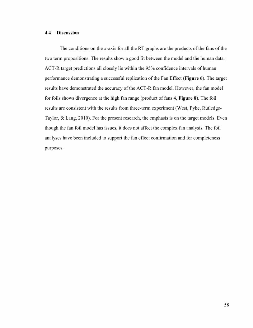
58

4.4 Discussion

The conditions on the x-axis for all the RT graphs are the products of the fans of the

two term propositions. The results show a good fit between the model and the human data.

ACT-R target predictions all closely lie within the 95% confidence intervals of human

performance demonstrating a successful replication of the Fan Effect (Figure 6). The target

results have demonstrated the accuracy of the ACT-R fan model. However, the fan model

for foils shows divergence at the high fan range (product of fans 4, Figure 8). The foil

results are consistent with the results from three-term experiment (West, Pyke, Rutledge-

Taylor, & Lang, 2010). For the present research, the emphasis is on the target models. Even

though the fan foil model has issues, it does not affect the complex fan analysis. The foil

analyses have been included to support the fan effect confirmation and for completeness

purposes.

59

4.5 Conclusion

The successful replication of the Fan Effect results by the ACT-R fan analytical

model served to address the following important concerns in the modeling method and tools

used in this research:

(1) Sample size

Is the sample size too small to provide reasonable data? The replication of Fan effect shows

that the sample size is sufficient to provide reasonable data.

(2) Counterbalance dataset

Is the design of the datasets used in these experiments counterbalanced? This is a critical

factor for fan models. The design of the dataset for Experiment 1 must be counterbalanced

in order to obtain the Fan Effect; since the datasets for the subsequent experiments have the

same design, the assumption of counterbalance is likely to hold for the other experiments.

(3) Validity of the tools and method

The experiment apparatus, support tools and learning method (fill-in–the-blanks learning

and qualifying test as a method) are new approaches. Will they work together? The results

of Experiment 1 show that these tools are working together and were able to provide input

that led to a successful analysis, and that they are in agreement with the ACT-R theory and

human data.

(4) Integrity of the test and analysis process

Will the recognition test, the data collection, and the analysis process for the complex fan

experiments work together? The successful replication of the Fan Effect in Experiment 1

has provided some assurance of integrity for the test and analysis process for the rest of the

complex fan experiments.

(5) Another important implication of the replication of the Fan Effect is that, the parameter

values used in Experiment 1 can now be used for the zero parameter modeling for the later

models used in this research.

60

In conclusion, Experiment 1 has served as a preliminary step for proposition learning

and it has also provided a reasonable assurance of the integrity of the design, the method,

and the tools for this research.

61

Experiment 2: Container-Location Experiment 5 Chapter:

Experiment 2 was the container-location experiment. Experiment 2 evaluated the

effects of overlapping datasets. According to Anderson‟s fan model there are two

possibilities of identifying the number of fans for the fan effect in Experiment 2. Either the

fan is derived from a standalone set of facts (Experiment 2) or the fan is derived from a

combined set of facts (Experiment 1 & 2).

The propositions used in Experiment 2 were three-word phrases that had a format of

“container in location” where the container concepts were the same containers used in

Experiment 1. The size of the dataset was 26 propositions. Experiment 2 enabled the

participants to learn the second installment of propositions for the inference task.

Experiment 2 was also designed to ease up on the learning of the needed propositions for the

inference experiment.

5.1 Method

5.1.1 Participants

The same 10 participants as described in Experiment 1

5.1.2 Materials

Two integrated software modules were developed to test and collect test data and to

ensure test records contain correct fan information and ACT-R predictions (target):

1) The OCLearn module (Appendix F.1) was used for the learning and qualifying

phases.

2) The container-location Experiment module (CLE; Appendix F.3) was the

apparatus used for the recognition test.

Experiment 2 test data consisted of 26 two-term (2 content words) propositions.

Each proposition paired a container with a location. The container term was the same

62

containers used in Experiment 1. The propositions were designed with different fan

combinations. For examples, 1-1 (the container and location occur uniquely in only one

sentence), 2-1, (container occurs in one other sentence), 1-2 (the location occurs in one other

sentence), 2-2, and 3-1. For the recognition test there were 26 target and 26 foil probes. The

details of the test data were shown in Table 4.

Material Studied Target Probes Foil Probes

box in pool

car in cave

purse in cave

cup in church

bag in church

tube in church

coat in bank

safe in office

tent in office

case in garden

case in yard

trunk in garden

bucket in garden

drawer in kitchen

shelf in library

tray in library

pants in yard

drawer in yard

bowl in yard

tank in river

bottle in court

plate in court

pot in forest

pot in park

bowl in forest

envelop in forest

box in pool

car in cave

purse in cave

cup in church

bag in church

tube in church

coat in bank

safe in office

tent in office

case in garden

case in yard

trunk in garden

bucket in garden

drawer in kitchen

shelf in library

tray in library

pants in yard

drawer in yard

bowl in yard

tank in river

bottle in court

plate in court

pot in forest

pot in park

bowl in forest

envelop in forest

box in cave

car in pool

purse in church

cup in bank

bag in bank

tube in bank

coat in office

safe in garden

tent in garden

case in kitchen

trunk in kitchen

bucket in kitchen

drawer in library

shelf in yard

tray in yard

pants in river

drawer in river

bowl in river

tank in court

bottle in forest

plate in forest

pot in pool

pot in cave

bowl in cave

envelop in church

Table 4 Dataset Used in Experiment 2 Container-Location

63

5.1.3 Procedures

Each participant received verbal instructions at the beginning of Experiment 2. There

were three phases in Experiment 2. In Phase 1, the learning phase, participants studied 26

propositions (targets). The learning process involved: the study of 3 propositions at a time

and then the completion of a fill-in-the-blank test for the 3 propositions. The participant

moved to the next 3 propositions when the fill-in-the-blank test achieved 100% accuracy.

This learning process ensured a level of learning of the propositions for the qualification test

in phase 2.

Phase 2 was the qualification test, where participants were tested for accuracy on a

fill-in-the-blank test for the entire set of test data. Participants had to achieve minimum 90%

accuracy before they could proceed to the recognition test. Both phase 1 and 2 were

administered automatically by the OCLearn module. Once the participant had completed the

qualification test, verbal instructions were given to the participant regarding the recognition

test in phase 3.

Phase 3 was the recognition test which began with a screen of instructions. It was

followed by a 2 seconds fixation cue. 26 target and 26 foil probes were presented to each

participant; each participant had to respond as quickly as possible by pressing a key labeled

in green (“L” key) if he or she recognized that the probe was from the study set (target), or

pressed the red labeled key (“A” key) if the probe did not belong to the study set (foil).

After each key-press response there was a 2 seconds pause before the next probe appeared.

Reaction time was measured and recorded. The recognition test was administered

automatically by the CLE module.

5.2 Models construction

64

The analytical model for Experiment 2 was based on fan analysis (Equation 9). The

RT function used to calculate reaction time is the same as in Experiment 1. However, there

were two possible sets of fan-combinations that could be used as input to predict the

reaction times for Experiment 2. The first scenario was the “standalone” scenario; the fan

combination for this scenario treated Experiment 2 as an independent experiment that was

the fan combinations used to calculate the predictions were independent of Experiment 1.

For example, the proposition “box in pool” had a fan combination of 1-1 that meant the

container “box” and the location “pool” was considered to have only one association. The

second scenario was the “combined” scenario; the fan combination for this scenario treated

Experiment 2 as a continuation of Experiment 1. The fan combinations used to calculate the

predictions were based on the total propositions from Experiment 1 and 2. For example, the

proposition “box in pool” had a fan combination of 2-1 since “box” had two associations. It

was associated with “ring in box” and “box in pool”. The analytical model with two

scenarios was constructed with MS Excel. All parameters used were the same as in

Experiment 1.

5.3 Results

The reaction time analysis compares human recognition test results to two models:

1) the standalone fan model where the fans were calculated based on the propositions used

in Experiment 2 alone. 2) The combined fan model where the fans were calculated based on

the propositions used in both Experiment 1 and 2. The two model comparisons were

necessary due to the uncertainty of the dataset boundaries for Experiment 2, and that a clear

determination of the fan calculations is critical for modeling Experiment 3. The analysis for

65

each model also covers 1) all data comparison and 2) “outliers removed” comparison.

Following the same approach used in Experiment 1, to maximize power for measurement,

the conditions on the x-axis for all the RT graphs represent the products of fans for which

ACT-R makes the same reaction time predictions. All of the parameters in the ACT-R

models were the same as in Experiment 1. The error bars associated with the human data in

RT analyses show the 95% confidence intervals for the human performance.

5.3.1 Error analysis

Figure 9 and 10 show error analysis for Experiment 2 in terms of percentage of error

and error count for targets (in blue). The errors for small fan combination, the error rates are

below 5% and the larger fan combinations are below 10% with the exception of the 4-3

0%

5%

10%

15%

20%

25%

30%

35%

1-2 2-1 1-3 2-2 3-1 2-3 3-2 4-1 2-4 3-3 4-2 3-4 4-3 4-4

Pe

rce

nt

of

err

or

Fan Combination

% Target

% Foil

Figure 25 Experiment 2 error (%) analysis

Figure 9 Experiment 2 error percentage analysis

66

combination. The apparent high percentage for 4-3 is largely due to the smaller number of

samples in the experiment for 4-3. The actual error count is 3 out of 10 records. So, the

impact on the RT analysis is small. Overall the error rates are consistent with the learning

method and expectation.

Figure 9 and 10 also show the foil error analysis (in red) for Experiment 2 in terms

of percentage of error and error count. The errors for small fan combination, the error rates

are below 6% which is similar to the target rates. But for the larger fan combinations the

error rates show a much higher gradient, they range from 15% to 30%. However, the 30%

error has an actual error count of 3 out of 10 records. So, in real terms, there were only three

0

1

2

3

4

5

6

1-2 2-1 1-3 2-2 3-1 2-3 3-2 4-1 2-4 3-3 4-2 3-4 4-3 4-4

Erro

r co

un

t

Fan Combination

Target

Foil

Figure 10 Experiment 2 error count analysis

67

errors out of 235 foil records. The impact on the RT analysis is small. Overall the error rates

are consistent with the learning method and expectation.

5.3.2 Target Analysis

Figure 11 shows the standalone target reaction time analysis relative to the

combined mode with all the data recorded for the Experiment 2. Figure 12 shows the

standalone target reaction time analysis relative to the combined mode with the outliers

removed for the Experiment 2. Outliers are reaction times that are more than two standard

deviations away from the mean. There were 13 outlier records removed out of 221 records.

All of the outliers had a longer reaction time than the mean, indicating the anomalies were

due to hesitations or second guessing. The removal of the outliers had two effects: 1) it had

slightly lowered the affected means and 2) it had increased the resolutions for 95%

confidence intervals; the affected confidence intervals became smaller. Overall, the fit was

improved. Figure 12a shows the independent (not compared to the combined mode)

standalone target reaction time analysis with the outliers removed for the Experiment 2.

Figure 12a presents reaction times according to the standalone mode products of fans.

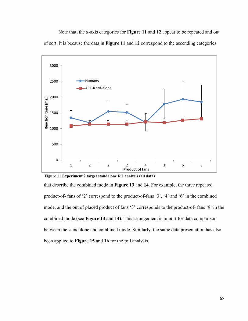
68

Note that, the x-axis categories for Figure 11 and 12 appear to be repeated and out

of sort; it is because the data in Figure 11 and 12 correspond to the ascending categories

that describe the combined mode in Figure 13 and 14. For example, the three repeated

product-of- fans of „2‟ correspond to the product-of-fans „3‟, „4‟ and „6‟ in the combined

mode, and the out of placed product of fans „3‟ corresponds to the product-of- fans „9‟ in the

combined mode (see Figure 13 and 14). This arrangement is import for data comparison

between the standalone and combined mode. Similarly, the same data presentation has also

been applied to Figure 15 and 16 for the foil analysis.

0

500

1000

1500

2000

2500

3000

1 2 2 2 4 3 6 8

Re

acti

on

tim

e (

ms.

)

Product of fans

Humans

ACT-R std-alone

Figure 11 Experiment 2 target standalone RT analysis (all data)

69

0

500

1000

1500

2000

2500

1 2 2 2 4 3 6 8

Re

acti

on

tim

e (

ms.

)

Product of fans

Humans

ACT-R standalone

Figure 12 Experiment 2 target standalone RT analysis (outliers removed)

Figure 23 Experiment 2 target standalone RT analysis

0

500

1000

1500

2000

2500

1 2 3 4 6 8

Re

acti

on

tim

e (

ms.

)

Product of fans

Humans (standalone, ordered)

ACT-R standalone

Figure 12a Experiment 2 target standalone RT analysis (in ordered fan products; outliers removed)

70

Figure 13 shows the combined fan model target reaction time analysis with outliers

and Figure 14 shows the combined fan model target reaction time analysis without the

outliers.

As in Experiment 1, removing the outliers produced a better fit. Visually, both the

stand-alone model and the combined model, with the outliers removed, did a reasonable job

of fitting the data, but the combined model appeared to fit better. To get an idea of whether

or not this difference was due to chance a simple t-test was performed on the difference

between each model‟s prediction and each participant‟s actual reaction time. More

specifically, this was a two tailed, paired t-test was performed on the differences between

the model prediction and the subjects RT time on every trial (with outliers removed). This

provided two average difference scores for each model. With the outliers included the

average difference scores were 154 for combined fan and 200 for standalone fan. This

difference was significant at P<0.001, with the outliers removed the average difference

scores were 85 for combined fan and 166 for standalone fan. This difference was significant

at P<0.001.

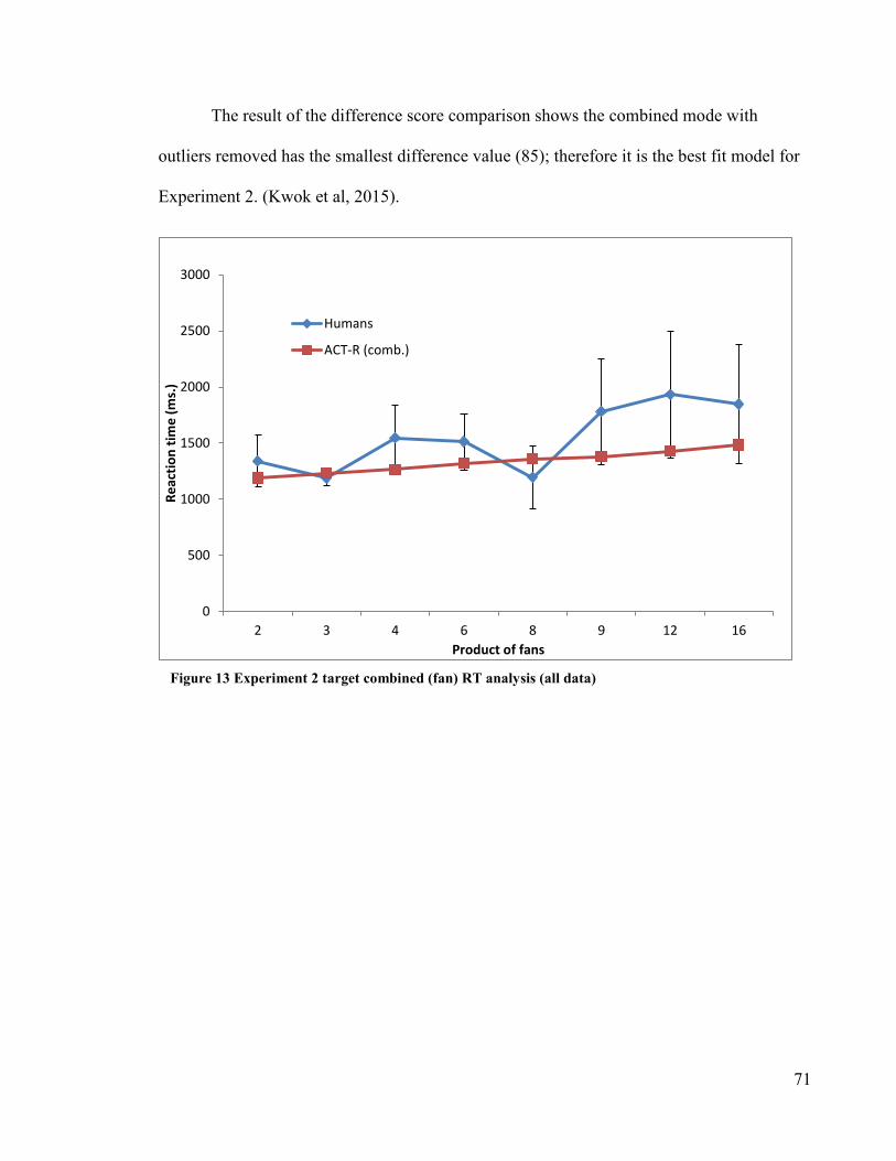
71

The result of the difference score comparison shows the combined mode with

outliers removed has the smallest difference value (85); therefore it is the best fit model for

Experiment 2. (Kwok et al, 2015).

0

500

1000

1500

2000

2500

3000

2 3 4 6 8 9 12 16

Re

acti

on

tim

e (

ms.

)

Product of fans

Humans

ACT-R (comb.)

Figure 13 Experiment 2 target combined (fan) RT analysis (all data)

72

5.3.3 Foil Analysis

The foil reaction time analysis also compares human recognition foil results to two

fan models: 1) the standalone fan model where the fans were calculated based on the

propositions used in Experiment 2 alone. 2) The combined fan model where the fans were

calculated based on the propositions used in both Experiment 1 and 2. Figure 15 shows the

standalone ACT-R foil model reaction time analysis (relative to the combined mode) with

all the data recorded from the Experiment 2. Figure 16 shows the standalone foil model

reaction time analysis (relative to the combined mode) with the outliers removed. There

were 12 outlier removed out of 235 records. All of the outliers had a longer reaction time

than the mean, showing the anomalies were mostly due to hesitations. The removal of the

outliers had two practical effects: 1) it had slightly lowered the affected means and 2) it had

0

500

1000

1500

2000

2500

2 3 4 6 8 9 12 16

Re

acti

on

tim

e (

ms.

)

Product of fans

Humans

ACT-R (comb.)

Figure 14 Experiment 2 target combined (fan) RT analysis (outliers removed)

73

increased the resolutions for 95% confidence intervals; the affected confidence intervals

Figure 16 Experiment 2 foil standalone RT analysis (outliers removed)

Figure 23 Experiment 2 target standalone RT analysis

1000

1100

1200

1300

1400

1500

1600

1700

1800

1900

2000

1 2 2 4 4 3

Re

acti

on

tim

e (

ms.

)

Product of fans

Humans

ACT-R std-alone

Figure 15 Experiment 2 foil standalone RT analysis (all data)

1000

1200

1400

1600

1800

2000

1 2 2 4 4 3

Re

acti

on

tim

e (

ms.

)

Product of fans

Exp2 Foil, Human vs. Stand-alone (no outliers)

Humans

ACT-R std-alone

74

became smaller. With the outliers removed, the results still show all but one foil predictions

fell outside the 95% confidence intervals of the human data.

Figure 16a shows the independent (not compared to the combined mode)

standalone foil reaction time analysis with the outliers removed for the Experiment 2.

Figure 16a presents Experiment 2 foil reaction times according to the standalone mode

products of fans.

The combined fan foil model for Experiment 2 used the datasets from Experiment 1

and 2 combined to calculate fan combinations for the analysis. Figure 17 shows the

combined fan model foil reaction time analysis with all the data. The results show foil

predictions fell completely within the 95% confidence intervals of the human data. Figure

18 shows the combined fan model foil reaction time analysis with the outliers removed for

the Experiment 2. Again, there were 11 outlier records removed from 235 records. All of the

1000

1200

1400

1600

1800

2000

1 2 3 4

Re

acti

on

tim

e (

ms.

)

Product of fans

Humans

ACT-R standalone foil

Figure 16a Experiment 2 foil standalone RT analysis (in ordered fan products; outliers removed)

Figure 23 Experiment 2 target standalone RT analysis

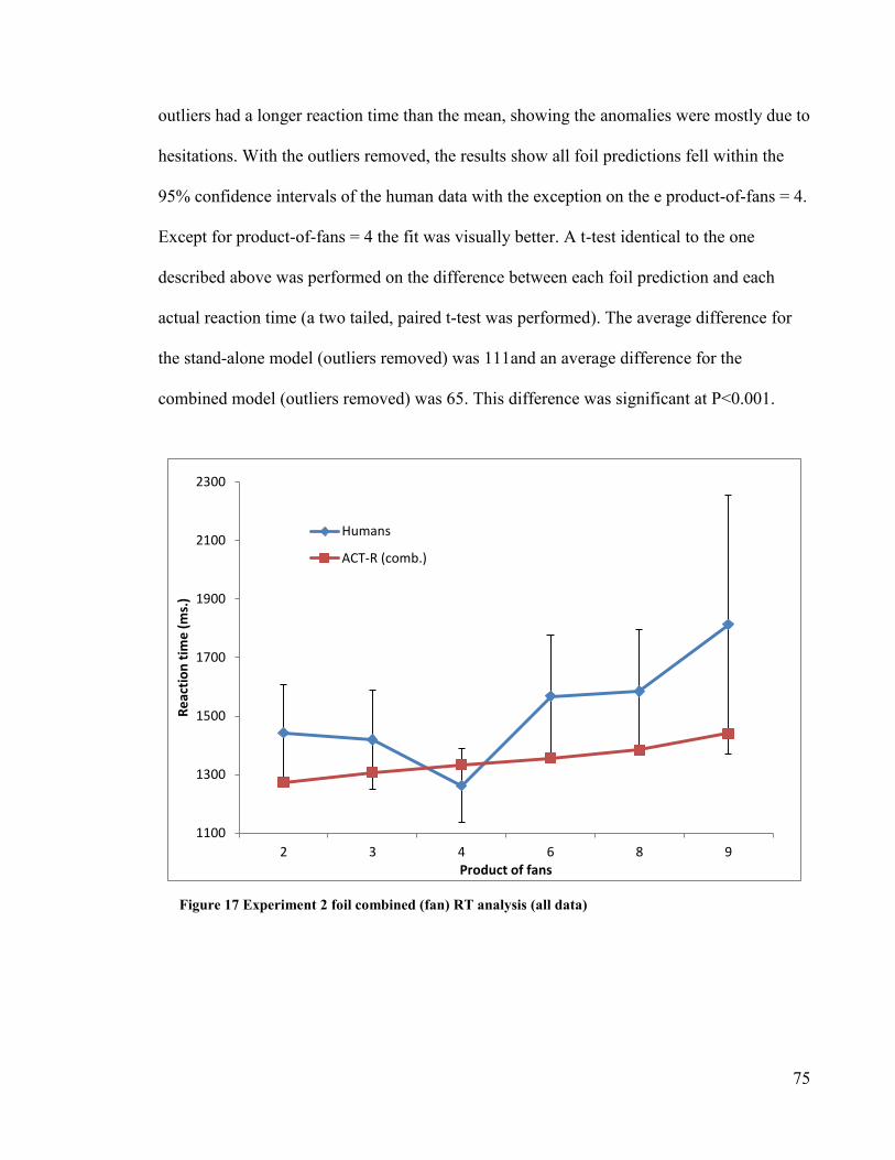
75

outliers had a longer reaction time than the mean, showing the anomalies were mostly due to

hesitations. With the outliers removed, the results show all foil predictions fell within the

95% confidence intervals of the human data with the exception on the e product-of-fans = 4.

Except for product-of-fans = 4 the fit was visually better. A t-test identical to the one

described above was performed on the difference between each foil prediction and each

actual reaction time (a two tailed, paired t-test was performed). The average difference for

the stand-alone model (outliers removed) was 111and an average difference for the

combined model (outliers removed) was 65. This difference was significant at P<0.001.

1100

1300

1500

1700

1900

2100

2300

2 3 4 6 8 9

Re

acti

on

tim

e (

ms.

)

Product of fans

Humans

ACT-R (comb.)

Figure 17 Experiment 2 foil combined (fan) RT analysis (all data)

76

1000

1200

1400

1600

1800

2000

2200

2 3 4 6 8 9

Re

acti

on

tim

e (

ms.

)

Product of fans

Exp2 Foil, Human vs. Combined (no outliers)

Humans

ACT-R (comb.)

Figure 18 Experiment 2 foil combined (fan) RT analysis (outliers removed)

77

5.4 Discussion

According to the ACT-R theory of spreading activation, activation spreads from the

constituent elements of a probe to the chunks stored in memory. The more spreading

activation received, the higher the activation of the chunk in memory. During retrieval, the

chunk with the highest activation is chosen and the retrieval time is proportional to its

activation level. The amount of activation spread from an element in the probe to a chunk in

memory is a function of the fans of the element. Specifically, the amount of activation

spread reflects the extent to which the element can be used to uniquely identify a chunk

(Anderson J. R., 2007, p.35). For example, if prior exposure were equal (i.e. the condition of

counterbalanced is satisfied), a probe element with a fan of 2 would have half the predictive

power of a probe element with a fan of 1. The replication of the fan effect in Experiment 1

has confirmed that the datasets for the complex fan experiments are all counterbalanced.

However, determining the size of the fan depends on the boundaries of the study set

(proposition dataset). This is because the probability that an element can uniquely identify a

chunk depends on how many other chunks the element occurs in. Therefore the definition of

the scope of the fan is very important. For Experiment 2, there are two possible definitions

for the scope of the dataset. The first possibility is the standalone fan scope; the standalone

scope for the fan is defined by all the facts in Experiment 2 alone. And the second

possibility is the combined fan condition; the combined scope is defined by all the facts in

Experiments 1 and 2 together. If the scope of the fan in Experiment 2 included the facts

from Experiment 1 then it would raise the fan of the containers since the same containers

appeared in both Experiment 1 and 2. The combined scope will result in higher fan and

reaction times. For example, the proposition “box in pool” in Experiment 2, the container

78

“box” if it were considered to be in standalone mode, the fan for “box” is 1 since there was

only one occurrence in Experiment 2. However, if it were in combined mode, the fan for

“box” would be increased to 2 since the combined mode would have included the additional

proposition “ring in box” from Experiment 1 (Kwok,West, Kelly, 2015).

Figures 12 to 19 show the reaction time comparisons for standalone and combined

scopes for targets and foils. The conditions on the x-axis are the products of the fans of the

terms in the probes as described in Experiment 1.

In general, the target results show a good fit between models and the human data for

both scenarios (standalone and combined) with an exception in the product of fans 8

condition. This particular condition is made up of only one proposition “pants in yard” and

it has only 10 data points. One possible explanation for this anomaly comes from the fact

that “pants” only appears once in Experiment 2, it has a fan of 1 in standalone condition,

therefore the participants might be quicker to identify the proposition “pants in yard” is true

due to the unique appearance of “pants” in Experiment 2. It is also generally observed that

any proposition which has only a fan of 1 will always illicit a quicker reaction time. It

suggests that human subjects might have a heuristic of remembering “fan of 1” items. This

same explanation is also applied to the anomaly observed in the foil analysis (product-of-

fans 4). The anomaly shows that participants were quicker to recognize fan 1 foils than the

model‟s prediction.

If we could discount the anomaly of condition product of fans 8, once again the fan

effect has been replicated in Experiment 2. All ACT-R predictions (target) tracked closely

with human performances and fall within the 95% confidence intervals of human data. The

standalone mode and combined mode comparisons were made because it is absolutely

79

crucial that the correct fan combination model (standalone or combined fan) be identified

since the inference model is predicated on the use of the correct fan-combinations. With all

the RT analyses, Figures 14 (targets) and 18 (foils) show a better fit for the combined scope

model since all of its target predictions fall within the 95% confidence intervals of the

human data and the similarly for the majority of the foil data. And this result confirms the

intuition that the participants had combined Experiment 1 and 2 into a single context

because the experiments were carried out in close succession.

The r-square statistic is a common statistic used to determine how well two sets of

data are correlated with each other. But for the scope issue, I need to determine first, if the

two models are statistically different and then if the models are statistically different which

model is a better descriptor; r-square is inadequate for such task.

To test for the fan scope issue statistically, the reaction time (RT) scores for each

subject were compared with the model predictions for both scopes. This was done by

subtracting the human RT scores from each scope‟s predicted RT scores for each trial. This

produced two difference scores for every trial, for every subject. The mean difference score

for the stand-alone model was 166 and the mean difference score for the combined model

was 85. Using a pairwise t-test we found that the difference scores for the combined and

standalone models were statistically significant (P<0.001) and the average for difference

scores for the combined model is also significantly smaller than the standalone average

difference - the combined average difference score is almost half of standalone average

difference (85 compared to 166). The calculated RMSD for the combined model was 164;

for the standalone model was 186. Both RMSD and the average difference scores were in

total agreement that the combined fan model is the best fit model for Experiment 2.

It is important also to note that in theory, the I, F and S parameters should have been

further adjusted for the overlapping dataset (for example, for the combined mode the fans

80

are derived based on the combined set of Experiment 1 and 2 propositions then S should

probably reflect that combined set as well. Making S = log 29+26 = log 55 = 1.74). But in

the interest of assessing the test results from a “zero parameter” modeling perspective, the

F and S parameters have been assumed to be constants – i.e. the changes were assumed to

be negligible. This assumption will be revisited in the future analysis.

5.5 Conclusion

The analysis suggests that, even though Experiment 1 and Experiment 2 were

separate experiments (where dataset boundaries are concerned), the scope for Experiment

2‟s dataset follows a combined fan model. Through the usage of triangulation techniques i.e.

difference average analysis, RMSD (the smaller the value the better the model), and the

target and foil RT analyses, the results support the conclusion that the combined fan model

is a better assumption for the inference model construction for Experiment 3.

Another important conclusion is that Experiment 2 has also replicated the Fan Effect

and therefore the results continue to support all of the assumptions for the complex fan

experiments; the participants have completed the learning of the second set of propositions

for Experiment 3.

81

Experiment 3 – Object-Location (inference test) 6 Chapter:

Experiment 3 was the inference test for the complex fan inference experiment.

Experiment 3 demonstrated that overlapping information can be used to make inferences

from associated facts. Experiment 3 was conducted immediately after Experiment 2. The

experiment consisted of just a single recognition test phase. Participants in Experiment 3

were presented with probes that had a format of “object in location.” The objects and the

locations were the same objects and locations that the participants had learned in

Experiment 1 and 2. Participants were asked to recognize if a probe was true or false based

on what they had learned from Experiment 1 and 2. That is, they needed to combine the

information from Experiment 1 (object-container) with the information from Experiment 2

(container-location) to make a judgment on whether a probe of object in location was true.

6.1 Method

6.1.1 Participants

The participants were the same six male and four female volunteers from

experiments 1 and 2.

6.1.2 Materials

The complex fan experiment (CFE) module was used for the recognition test. CFE

(Appendix F.4) automated the inference recognition test procedure. There were 48 probes

for each participant. The details of the probes are shown in Table 5.

82

Material Studied Target Probes Foil Probes

ring in pool

watch in cave

pen in cave

key in church

shoes in church

hat in church

spoon in bank

brush in bank

comb in office

mouse in office

dog in office

cat in office

book in garden

gloves in garden

scarf in garden

pearl in garden

coin in garden

letter in garden

battery in kitchen

banner in library

book in yard

lamp in river

lamp in court

eye-glasses in forest

ring in cave

watch in cave

watch in pool

pen in pool

key in cave

shoes in cave

hat in pool

spoon in church

brush in church

comb in church

mouse in bank

dog in bank

cat in church

book in pool

gloves in bank

scarf in pool

pearl in church

coin in office

letter in kitchen

battery in deck

banner in deck

banner in yard

book in river

lamp in yard

lamp in kitchen

eye-glasses in yard

6.1.3 Procedure

Explicit instructions were given to each participant before the experiment began. The

participant was instructed to expect probes with a format “object in location” and the objects

and locations were the same objects and locations that he or she had previously learned in

Table 5 Material Used in Experiment 3 (CFE)

83

Experiment 1 and 2. He or she was to use the object as a cue to identify the associated

container and then confirm if the container was associated with the location in his or her

mind.

Following the verbal instructions the CFE module was launched for the recognition

test. The recognition test steps were the same steps used in recognition tests for Experiment

1 and 2. 24 target and 24 foil probes were presented to each participant automatically; each

participant had to respond as quickly as possible by pressing a key labeled in green (“L”

key) if he or she recognized that the probe was true or pressed the red labeled key (“A” key)

if the probe was not true (foil).

The CFE module began with a screen of instructions. It was followed by a 2 seconds

fixation cue and then a probe was presented. After each key-press response there was a 2

seconds pause before the next probe appeared. Reaction time was measured for each probe.

6.2 Model Construction: ACT-R model for complex fan

ACT-R has two ways to retrieve facts from memory. The first way is to retrieve a

match for a fact that has been presented (as in the models for Experiments 1 and 2). The

second way is to construct a query by using a partial fact as a cue to retrieve a complete fact.

For example, if the apple was in the bucket, the retrieval cue “apple ?” would retrieve apple

bucket. In this case the fan is based on the elements present in the query (so the fan of

apple). One way to extend the ACT-R fan model to model Experiment 3 is to use a query to

first retrieve a container for the object and then check to see if it‟s in the location.

Continuing with our example, if the target facts are “apple in bucket”, “bucket in yard” and

the probe is “apple in yard”, one would use “apple in ?” to retrieve “apple in bucket”, then

84

use “bucket in yard” to retrieve a match. The time for this would be the sum of the two

retrieval times, as determined by the fan, plus the time for the associated productions to

direct the actions, plus the times for perceptual and motor actions. We will refer to this as

the dual retrieval model. The dual retrieval model is the basis for Serial Complex Fan

Model (SCFM) which is an extended ACT-R model and it is fully compliant with the

current ACT-R theory.

However, there is another possibility, although the facts were learned separately in

Experiments 1 and 2 that does not necessarily mean they were stored separately. Subjects

could have realized that the new information learned in Experiment 2 was related to the

information learned in Experiment 1, leading them to store the new information as three

element chunks (i.e., object container location). In this case, both the object and the location

can be used as a cue to retrieve a container. This would only require one retrieval and, since

activation would spread from both the object and the location, this single retrieval would be

faster than the query retrieval in the dual retrieval model. We will refer to this as the single

retrieval model. This is the basis for the Parallel Complex Fan Model (PCFM) also referred

to as the single retrieval model (see Appendix D.3) for detail construction. For the dual

retrieval model description which is referred to as Serial Complex Fan Model (SCFM; see

Appendix D.1).

6.2.1 SCFM and search

Unlike the single retrieval model, which follows the logic of other ACT-R fan

models such that only one memory retrieval production is needed to determine if a probe is

a target or a foil, the dual retrieval situation is more complex. In the dual retrieval model

(SCFM basic), there is no way to know if the first query retrieved the right container until

85

the result of the subsequent match is evaluated. Under these conditions it makes sense to

consider an ACT-R model that uses a search strategy. That is, if it fails to make a match it

goes back and tries a different query until either it correctly identifies the probe as a target or

the search is exhausted. For example, the first query using the object cue “object in ?” can

potentially retrieve a wrong container, so the subsequent match may lead to an error in

judgment. The model would provide an answer “no” when the answer should have been a

“yes” according to the basic models. Under these conditions it is necessary to consider a

more realistic ACT-R model that uses a search strategy. That is, if a retrieved chunk fails to

make a match, it goes back and tries a different retrieval and does not decide the target is

false until the search is exhausted (this requires the use of the refraction function in ACT-R

to prevent the same retrieval from being made again). A similar search process of retry also

applies to the second query “container in ?”. For the more realistic search model, the SCFM

basic model has been extended to include the search steps described above. The extended

SCFM model shall be referred to as SCFM search model.

6.2.2 SCFM Search Model

SCFM model is a zero parameter ACT-R compliant analytical model. This model

assumes that the correct chunks are retrieved and therefore provides an estimate of the

fastest possible reaction time for this retrieval method. However, because Anderson‟s foil

detection model cannot be applied to the initial query retrieval, it creates a state of

uncertainty where the subject cannot be sure if the probe is a foil or if further search is

needed. In this section, I will describe the extension of the basic SCFM to include search

time. The additional search time for SCFM is specified as the maximum number of attempts

86

for the two memory retrieval productions in the model. The number of attempts for the first

production is the number of attempts for the “object in ?” query. The number of attempts is

related to the number of connections that an object has. The number of connections that an

object has in a dataset is its fan. So the worst case scenario for tries for the object query is

the query time multiplied by the object‟s fan. Similarly for the second production, the

container query. The worst case scenario for tries (maximum number of attempts) for the

container query is the query time multiplied by the container‟s fan. The sample calculations

for the SCFM search model are described in Appendix D.5.

6.3 Results

6.3.1 Error analysis

Figures 19 and 20 show the number of errors in Experiment 3 which are within the

expected range of errors. For small fan combinations it is below 6% and for the larger fan

combinations the highest number of error is 6 for target (target is the focus of this research).

0

2

4

6

8

10

12

1-1-1 1-1-2 1-2-1 2-1-1 1-1-3 1-2-2 1-3-1 3-1-1 1-2-3 1-3-2 3-2-1 1-3-3 2-1-4 2-4-1 3-2-2 2-3-3 3-1-4 3-3-3 2-4-4

Nu

mb

er

of

err

or

Max. number of steps

target

foil

Figure 19 Experiment 3 error count analysis per fan combination

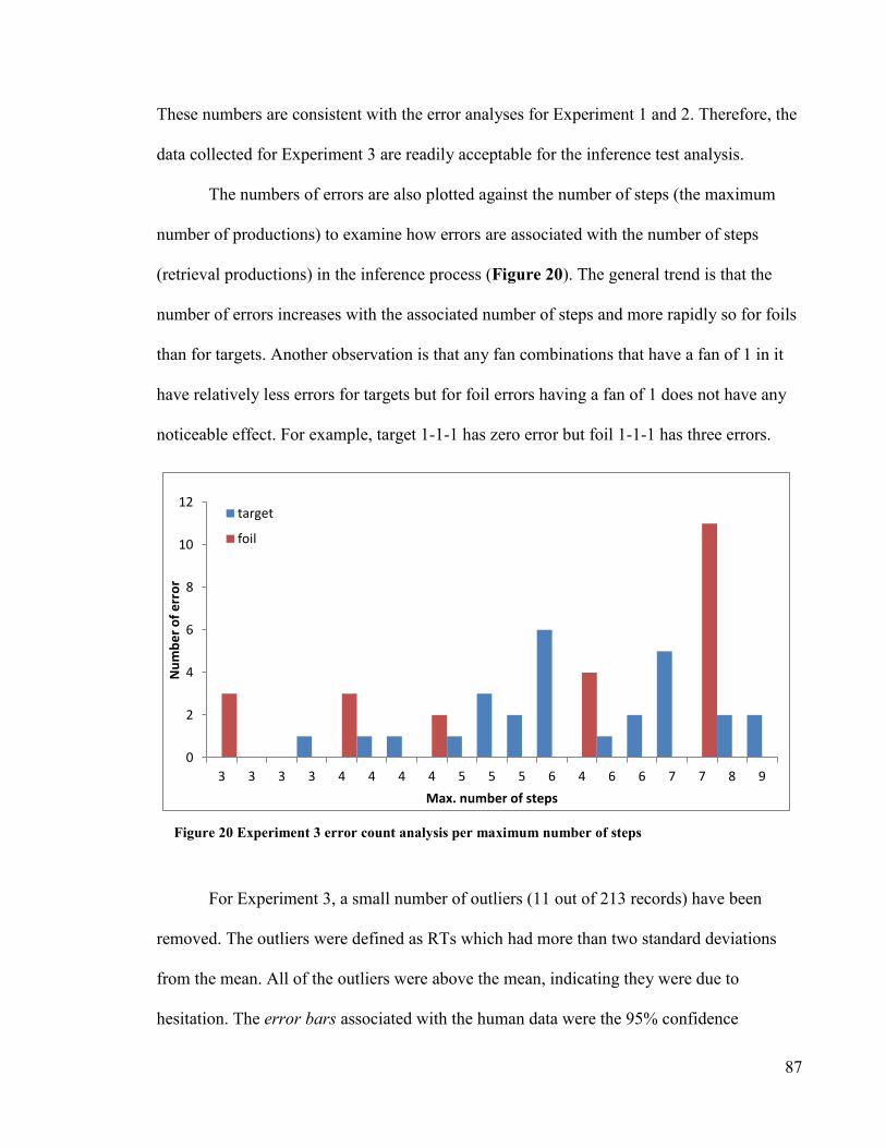
87

These numbers are consistent with the error analyses for Experiment 1 and 2. Therefore, the

data collected for Experiment 3 are readily acceptable for the inference test analysis.

The numbers of errors are also plotted against the number of steps (the maximum

number of productions) to examine how errors are associated with the number of steps

(retrieval productions) in the inference process (Figure 20). The general trend is that the

number of errors increases with the associated number of steps and more rapidly so for foils

than for targets. Another observation is that any fan combinations that have a fan of 1 in it

have relatively less errors for targets but for foil errors having a fan of 1 does not have any

noticeable effect. For example, target 1-1-1 has zero error but foil 1-1-1 has three errors.

For Experiment 3, a small number of outliers (11 out of 213 records) have been

removed. The outliers were defined as RTs which had more than two standard deviations

from the mean. All of the outliers were above the mean, indicating they were due to

hesitation. The error bars associated with the human data were the 95% confidence

0

2

4

6

8

10

12

3 3 3 3 4 4 4 4 5 5 5 6 4 6 6 7 7 8 9

Nu

mb

er

of

err

or

Max. number of steps

target

foil

Figure 20 Experiment 3 error count analysis per maximum number of steps

88

intervals for the human data. The x-axis for the graphs was arranged according to “total fan

“size (in brackets) and the fan combination in ascending order.

6.3.2 Target reaction time analysis for SCFM (basic model)

Figures 21 and 22 respectively show the reaction time (RT) analyses for the SCFM

basic model with all data and with outliers removed. Removing the outliers reduces the

means of the reaction times since all of the outliers are hesitation delays, and also reduces

the confidence intervals for human data.

0

1000

2000

3000

4000

5000

6000

7000

8000

9000

1-2-1 1-2-2 1-3-1 1-2-3 1-3-2 2-2-2 3-2-1 1-3-3 2-4-1 3-2-2 2-3-3 3-3-3 2-4-4

Re

acti

on

tim

e (

ms.

)

Fan combination

Humans

SCFM/ACT-R

Figure 21 Experiment 3 RT comparison: target, human and SCFM basic model (all data)

89

0

1000

2000

3000

4000

5000

6000

7000

8000

9000

1-2-1 (4)1-2-2 (5)1-3-1 (5)1-2-3 (6)1-3-2 (6)2-2-2 (6)3-2-1 (6)1-3-3 (7)2-4-1 (7)3-2-2 (7)2-3-3 (8)3-3-3 (9) 2-4-4(10)

Re

acti

on

tim

e (

ms.

)

Fan combination

Humans

SCFM/ACT-R basic

Figure 22 Experiment 3 RT comparison: target, human and SCFM basic model (outliers removed)

90

6.3.3 Target reaction time analysis for PCFM

Figure 23 shows the PCFM predictions for Experiment 3. It is compared to the

human data with outliers removed. All predictions are outside the confidence intervals of

human performance. The reaction times predicted are too quick for human performances.

0

1000

2000

3000

4000

5000

6000

7000

8000

9000

1-2-1 (4)1-2-2 (5)1-3-1 (5)1-2-3 (6)1-3-2 (6)2-2-2 (6)3-2-1 (6)1-3-3 (7)2-4-1 (7)3-2-2 (7)2-3-3 (8)3-3-3 (9) 2-4-4(10)

Re

acti

on

tim

e (

ms.

)

Fan combination

Humans

PCFM (single retrieval)

Figure 23 Experiment 3 reaction time (RT) comparison: target, human and PCFM basic model

(outliers removed)

91

6.3.4 Target reaction time analysis for SCFM search model

In general, the result of removing the outliers from the collected data reduces the

means of the reaction time since all of the outliers are hesitation delays that the outliers are

abnormal slow responses and there is no over-quick outlier response. Another consequence

of removing the outliers is the sizes of the confidence intervals would have been reduced

(human data in blue).These effects have applied to the SCFM search model (Figure 24 and

25). The comparisons show that the removal of the outliers has not distorted the integrity of

the collected data but has improved the resolution for model evaluation by the reduction of

the confidence intervals. So the subsequent comparisons will only apply to data with outliers

removed (see human data in Figure 26).

0

1000

2000

3000

4000

5000

6000

7000

8000

9000

1-2-1(4)

1-2-2(5)

1-3-1(5)

1-2-3(6)

1-3-2(6)

2-2-2(6)

3-2-1(6)

1-3-3(7)

2-4-1(7)

3-2-2(7)

2-3-3(8)

3-3-3(9)

2-4-4(10)

Re

acti

on

tim

e (

ms.

)

Fan combination

Humans

SCFM/ACT-R (max.)

Figure 24 Experiment 3 RT comparisons: target, human and SCFM search model (all data)

92

0

1000

2000

3000

4000

5000

6000

7000

8000

9000

1-2-1(4)

1-2-2(5)

1-3-1(5)

1-2-3(6)

1-3-2(6)

2-2-2(6)

3-2-1(6)

1-3-3(7)

2-4-1(7)

3-2-2(7)

2-3-3(8)

3-3-3(9)

2-4-4(10)

Re

acti

on

tim

e (

ms.

)

Fan combination

Humans

SCFM/ACT-R (max.)

Figure 25 Experiment 3 RT comparisons: target, human and SCFM search model (outliers removed)

93

6.3.5 Foil reaction time analysis

Since Anderson‟s fan model does not describe complex fan foil. Figure 26 (the foil

data graph) is included here for completeness and speculative evaluation. The human foils

are compared to foil estimates that are based on ACT-R multi-step basic foil model.

0

1000

2000

3000

4000

5000

6000

7000

8000

9000

1-1-1 1-1-2 2-1-1 1-1-3 3-1-1 2-1-4

Re

acti

on

tim

e (

ms.

)

Fan combination

Humans

ACT-R Foil

Figure 26 Experiment 3 RT comparisons: foil, human and ACT-R foil model

94

6.4 Discussion

The first set of models for Experiment 3 was the basic models which used only

spreading activation as a mechanism and they did not include search. The SCFM was a dual

retrieval model which represented classic ACT-R approach and PCFM was a single retrieval

model which represented the mental model approach. Both basic models described memory

retrieval as if subjects always retrieved the correct chunk on the first try. These basic models

were expected to produce a baseline of the fastest possible reaction times for the inference

task (Kwok,West, Kelly, 2015).

Figure 23 shows that the SCFM model trends with the human performance and the

model skirted the lower bound of the 95% confidence intervals of human data (as expected)

as there was no need for searching. The predictions coincided closely with the human data

e.g. fan combination 1-2-1. However, Figure 24 shows that PCFM predictions were too fast

compared to human performances. Every prediction was outside the 95% confidence

intervals of human data. To further quantify the relative fitness of these models, the Root

Mean Squared Differences (RMSD) was calculated. The smaller the difference (RMSD)

value the better fit is the model. So, the relative best fit model would have the smallest

RMSD. RMSD for PCFM and SCFM were 2216 and 1792 milliseconds respectively. Based

on these results, SCFM shows that it has a better fit than PCFM. Therefore, PCFM has been

eliminated from any further analysis.

The third model was the SCFM search model. The expectation was that the search

strategy would add time beyond the optimal response with the exception of the lowest fan

condition. This was because a fan of 1 of object and location guaranteed that the initial

query would produce the correct result. Figure 26 showed the SCFM search predictions.

95

The results showed that SCFM predicted the lowest fan combination exactly and with other

data points in good agreement with the human data.

The general trend of the reaction times shows a progressive increase according to the

increment of fan; the x-axis is arranged according to the total fan and sorted by object fan

and container fan. The valleys (the dips) in the graph show the double min-effect (from the

two combined two-term propositions) plus the relative shorter search time since the search

time is a function of the combinations of the object fan and container fan (see Appendix

D.5). The dips are the combined effect of shorter search time and min effect (discussed in

section 2.2.4 ).

6.5 Conclusion

The ACT-R spreading activation theory is a robust minimalist model which continues

to predict un-searched scenarios accurately in complex fan situations. ACT-R SCFM basic

model plus search time could provide a complete description for human data (within the

95% confidence intervals). The important findings with the ACT-R SCFM search model

are:

(1) The inference task defined in Experiment 3 is achieved via a (serial) dual retrieval

process (SCFM which is ACT-R‟s fan model) and not by a parallel single retrieval process

as in Radvansky‟s mental model approach (PCFM).

(2) The relational inference reaction times in Experiment 3 are the combined results of

spreading activation time (which is a function of fan) and search time. And spreading

activation theory alone (which is the basic building block of the fan model) cannot not

completely account for human performances. However, where there is no search involved

96

the spreading action prediction is very accurate; the example for this is the fan combination

of 1-2-1.

(3) For the search process, the search function could be rationalized as a function of the fans

of the related propositions that is, the search function is also fundamentally a fan function.

For Experiment 3, the search time is related to the number of attempts for the dual-retrieval

productions, and the number of attempts is related to object fan and container fan. The

explanation has been discussed in the model construction see Appendix D.

(4) The zero parameter extension of ACT-R (SCFM search) has successfully made

predictions that are consistent with human performances in that the predictions fall

consistently within the 95% confidence intervals of the human data. The successful results

of the complex fan experiments have demonstrated the accuracy and versatility of the ACT-

R theory, the complex fan paradigm, its tools and models.

(5) The foil prediction continues to raise issues. Figure 27 shows that the current foil

theory cannot explain the high fan results. Therefore, more research is needed in the foil

area.

Anderson's fan model seems to represent the simplest possible set of cognitive

mechanisms that can produce the fan effect. This does not effectively state that humans

never behave in more complex ways; if more complex processes do exist, they do not occur

automatically, but must be built around a fundamental process.

97

Experiment 4 - a follow-up experiment on dataset boundary 7 Chapter:

In Experiment 2, we identified an issue regarding the scope of the fan. The scope of

the fan is the set of the counterbalanced chunks used to determine the probabilities for

spreading activation. The main question is: what determines the dataset boundary for

complex fan experiments? For example, in Experiment 1 all other facts that a participant has

learned about the container „box‟ from before the experiment is assumed to be irrelevant to

the experiment, either because of exposure averages out across subjects or due to the strong

effect of the context of being in an experiment. If it is assumed that the previous exposure is

averaged out across subjects then the average effect of previous experiences is estimated as

a part of the F parameter. In Experiment 2, the facts learned in Experiment 1 were shown to

have an effect on the retrieval of facts learned in Experiment 2. This raised the following

questions: what factors define the scope of the fan in an experiment? And, how far does the

scope of the fan extend beyond the experiments? Experiment 4 is a follow-up experiment

which is designed to investigate the scope of fan over time.

The design of Experiment 4 was operationally identical to Experiment 1. Like

Experiment 1, Experiment 4 was a simple fan experiment. The key difference was in the

dataset and probes. The new dataset (test propositions) consisted of the same objects used in

Experiment 1. But in Experiment 4 these objects are associated with a color instead of a

container. To examine the time-lapse effect Experiment 4 was carried out 10 months after

the completion of Experiment 1 with the same participants. Since the variables between

Experiment 1 and 4 have been tightly controlled, the only free variable is the scope of the

fan. There are two possible outcomes: 1) The Fan Effect reaction times (from Experiment 4)

are more in line with the reaction times from Experiment 1 that is the fan sizes are not

98

adjusted (standalone) or 2) The Fan Effect reaction times are more in line with the reaction

times from the combined fan mode.

7.1 Method

7.1.1 Participants

The original participants from Experiment 1 were recruited.

7.1.2 Materials

To automate the learning, testing and data collation and collection, two integrated

software modules were developed:

1) Exp4learn.py and 2) Exp4.py

The details of the test data and probes are described in Table 6.

Material Studied Target Probes Foil Probes

ring is teal

banner is beige

lamp is brown

eye-glasses is beige

key is tan

hat is orange

spoon is yellow

battery is green

brush is pink

mouse is blue

lamp is pink

book is amber

eye-glasses is orange

scarf is amber

coin is violet

pearl is blue

ring is teal

banner is beige

lamp is brown

eye-glasses is beige

key is tan

hat is orange

spoon is yellow

battery is green

brush is pink

mouse is blue

lamp is pink

book is amber

eye-glasses is orange

scarf is amber

coin is violet

pearl is blue

ring is brown

eye-glasses is teal

banner is violet

lamp is orange

key is yellow

hat is blue

spoon is green

battery is amber

brush is beige

mouse is beige

lamp is orange

book is yellow

eye-glasses is violet

scarf is pink

pearl is orange

coin is yellow

99

battery is orange

lamp is violet

banner is yellow

book is pink

eye-glasses is amber

battery is orange

lamp is violet

banner is yellow

book is pink

eye-glasses is amber

battery is pink

lamp is beige

banner is tan

book is teal

eye-glasses is teal

7.1.3 Procedures

Before the start of the Experiment 4, each participant was given verbal instructions

about the experiment.

Similar to Experiment 1, Experiment 4 is composed of three phases. In phase 1,

participants study a set of “object is color” propositions using Exp4Learn. The learning

process involved: step 1 the study of 3 propositions at a time and step 2, the completion of a

fill-in-the-blank test for the 3 propositions. The participant moved to the next 3 propositions

when the fill-in-the-blank test achieved 100% accuracy. This ensured a level of learning of

the propositions for the qualification test in phase 2.

Phase 2 was the qualification test, where participants were tested for accuracy on a

fill-in-the-blank test for the entire set of test data. Participants had to achieve minimum 90%

accuracy before they could proceed to the recognition test. Both phase 1 and 2 were

administered automatically by the Exp4learn module.

Phase 3, Exp4.py is used for the recognition test. The procedure was similar to the

recognition test in Experiment 1 and 2. First, verbal instructions were given to the

participant. Following the verbal instructions the Exp4 module was launched for the

recognition test. The recognition test steps were the same steps used in recognition tests for

Experiment 1. 21 target and 21 foil probes were presented to each participant automatically;

each participant had to respond as quickly as possible by pressing a key labeled in green

Table 6 Material used in Experiment 4 (standalone)

100

(“L” key) if he or she recognized that the probe was true or pressed the red labeled key (“A”

key) if the probe was not true (foil).

The Exp4 module began with a screen of instructions. It was followed by a 2 seconds

fixation cue and then a probe was presented. After each key-press response there was a 2

seconds pause before the next probe appeared. Reaction time was measured for each probe.

The recognition test was administered automatically by the Exp4 module.

7.2 Model Construction

Two analytical fan models were constructed for comparisons. The standalone fan

model was based on Table 6 and the combined fan model was based on Table 7. The

combined dataset included the material studied in Experiment 1 as well as material studied

in Experiment 4 to simulate a different dataset boundary for Experiment 4. The objective of

the comparisons was to identify which dataset or scope is more compatible with human

performance.

Table 7 Material used in Experiment 4 combined fan simulation

Material Studied Target Probes Foil Probes

ring in box

watch in car

pen in purse

key in cup

shoes in bag

hat in tube

spoon in coat

brush in coat

comb in safe

mouse in safe

dog in tent

cat in tent

book in case

ring is teal

banner is beige

lamp is brown

eye-glasses is beige

key is tan

hat is orange

spoon is yellow

battery is green

brush is pink

mouse is blue

lamp is pink

book is amber

eye-glasses is orange

ring is brown

eye-glasses is teal

banner is violet

lamp is orange

key is yellow

hat is blue

spoon is green

battery is amber

brush is beige

mouse is beige

lamp is orange

book is yellow

eye-glasses is violet

101

gloves in case

scarf in trunk

pearl in trunk

coin in bucket

letter in bucket

battery in drawer

battery in pants

banner in shelf

banner in tray

book in drawer

lamp in tank

lamp in basket

lamp in bottle

eye-glasses in pot

eye-glasses in bowl

eye-glasses in urn

ring in teal

eye-glasses in beige

banner in beige

lamp in brown

key in tan

hat in orange

spoon in yellow

battery in green

brush in pink

mouse in blue

lamp in pink

book in amber

eye-glasses in orange

scarf in amber

pearl in blue

coin in violet

battery in orange

lamp in violet

banner in yellow

book in pink

eye-glasses in amber

scarf is amber

coin is violet

pearl is blue

battery is orange

lamp is violet

banner is yellow

book is pink

eye-glasses is amber

scarf is pink

pearl is orange

coin is yellow

battery is pink

lamp is beige

banner is tan

book is teal

eye-glasses is teal

102

7.3 Results

The reaction time analysis compares human recognition results from Experiment 4

to two models: 1) the standalone fan model where the fans were calculated based on the

propositions used only in Experiment 4, and 2) The combined fan model where the fans

were calculated based on the propositions used in both Experiment 1 and 4 (since the

propositions for both dataset shared the same objects). The two model comparisons have

provided new information on how elapse time has affected fan effect and reaction time.

Following the same approach used in Experiment 1 and 2, to maximize power for

measurement, the conditions on the x-axis for all the RT graphs represent the products of

fans for which ACT-R makes the same reaction time predictions. All of the parameters in

the ACT-R models were the same as in Experiment 1. The error bars associated with the

human data in RT analyses show the 95% confidence intervals for the human performance.

7.3.1 Error analysis

Figure 27 and 28 show the error analysis for Experiment 4 in terms of percentage of

error and error count for targets (in blue). The distribution of percentage of error for

Experiment 4 is similar to Experiment 2. The errors for small fan combinations are below

5% and for the larger fan combinations are below 12%. The numbers of errors are consistent

with the qualifying test criterion of 90% accuracy. Another of observation is that any fan

combination that has a fan of 1 has relatively less errors; the number of error seems to be a

function of the minima of the fans in a chunk. For example, in Figure 28, the number of

error for 3-1 and 1-3 (4%) are less than the number of error in 2-2 (5%).

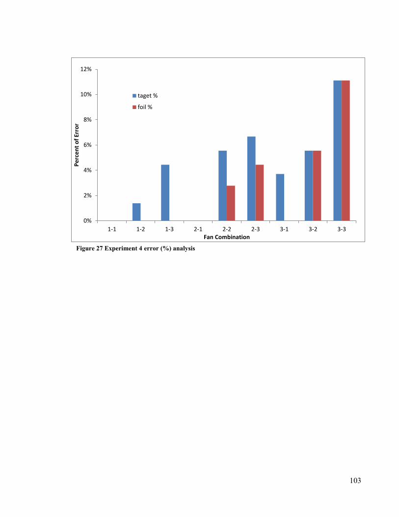
103

0%

2%

4%

6%

8%

10%

12%

1-1 1-2 1-3 2-1 2-2 2-3 3-1 3-2 3-3

Pe

rce

nt

of

Erro

r

Fan Combination

taget %

foil %

Figure 27 Experiment 4 error (%) analysis

104

Figure 27 and Figure 28 show foil error analysis for Experiment 4 in terms of

percentage of error and error count (in red). The error rates are below 10% at the higher fans

and no errors at all at the lower fans. Overall the error rates are consistent with the learning

method and expectation. The errors will not have any impact on the RT analyses.

7.3.2 Target Analysis

Figure 29 shows the standalone fan model target reaction time analysis with all the

data recorded for the Experiment 4. Figure 30 shows the standalone fan model target

reaction time analysis with the outliers removed for the Experiment 4. Outliers are reaction

times that are more than two standard deviations away from the mean. There were 9 outlier

records removed out of 168 records. All of the outliers had a longer reaction time than the

0

1

2

3

4

5

6

1-1 1-2 1-3 2-1 2-2 2-3 3-1 3-2 3-3

Nu

mb

er

of

err

or

Fan Combination

targets foil

Figure 28 Experiment 4 error count

105

mean, indicating the anomalies were due to hesitations or second guessing. The removal of

the outliers had two effects: 1) it had slightly lowered the affected means and 2) it had

increased the resolutions for 95% confidence intervals; the affected confidence intervals

became smaller. With the outliers removed, the results show all target predictions fell within

the 95% confidence intervals of the human data. Overall, the fit was improved.

800

900

1000

1100

1200

1300

1400

1500

1600

1700

1800

1 2 3 4 6 9

Re

acti

on

tim

e (

ms.

)

Product of fans

Humans

Stand alone

Figure 29 Experiment 4 RT comparison: target, human and “standalone” (all data)

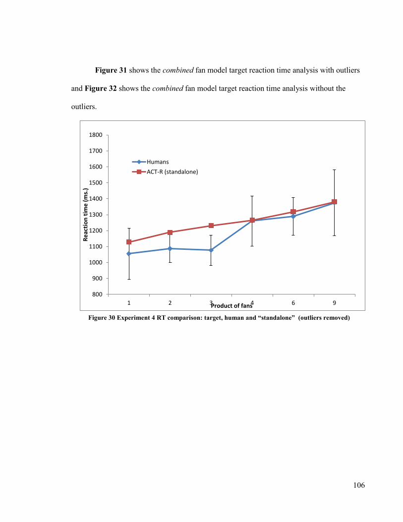
106

Figure 31 shows the combined fan model target reaction time analysis with outliers

and Figure 32 shows the combined fan model target reaction time analysis without the

outliers.

800

900

1000

1100

1200

1300

1400

1500

1600

1700

1800

1 2 3 4 6 9

Re

acti

on

tim

e (

ms.

)

Product of fans

Humans

ACT-R (standalone)

Figure 30 Experiment 4 RT comparison: target, human and “standalone” (outliers removed)

107

800

900

1000

1100

1200

1300

1400

1500

1600

1700

1800

2 4 6 8 12 18

Re

acti

on

tim

e (

ms.

)

Product of fans

Humans

Combined

Figure 31 Experiment 4 RT comparison: target, human and “combined” (all data)

800

900

1000

1100

1200

1300

1400

1500

1600

1700

1800

2 4 6 8 12 18

Re

acti

on

tim

e (

ms.

)

Product of fans

Humans

ACT-R (combined)

Figure 32 Experiment 4 RT comparison: target, human and “combined” (outlier removed)

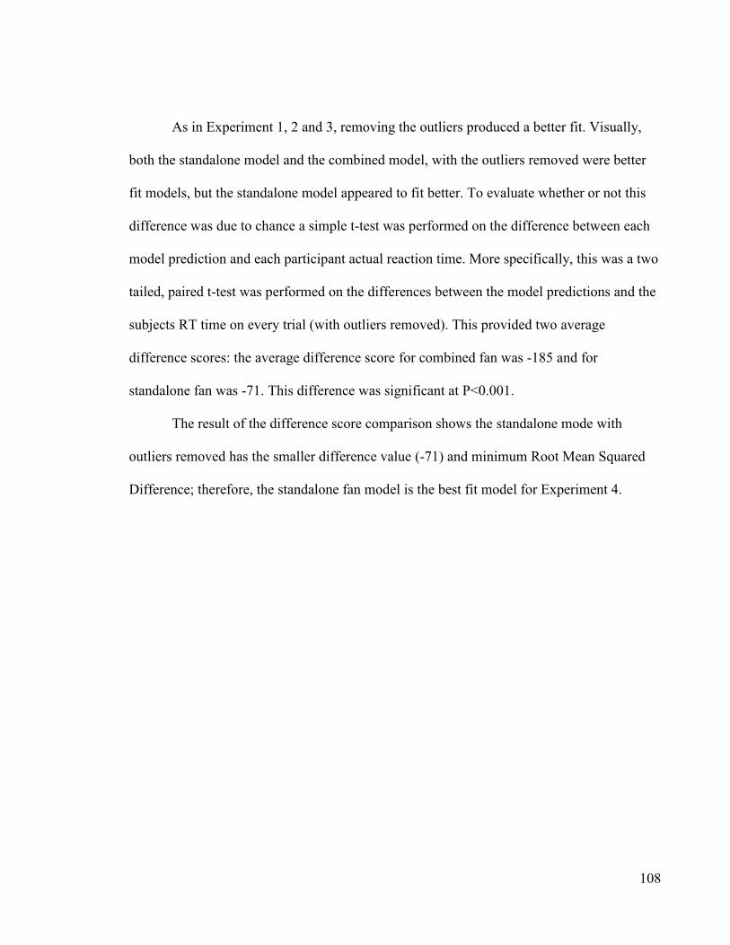
108

As in Experiment 1, 2 and 3, removing the outliers produced a better fit. Visually,

both the standalone model and the combined model, with the outliers removed were better

fit models, but the standalone model appeared to fit better. To evaluate whether or not this

difference was due to chance a simple t-test was performed on the difference between each

model prediction and each participant actual reaction time. More specifically, this was a two

tailed, paired t-test was performed on the differences between the model predictions and the

subjects RT time on every trial (with outliers removed). This provided two average

difference scores: the average difference score for combined fan was -185 and for

standalone fan was -71. This difference was significant at P<0.001.

The result of the difference score comparison shows the standalone mode with

outliers removed has the smaller difference value (-71) and minimum Root Mean Squared

Difference; therefore, the standalone fan model is the best fit model for Experiment 4.

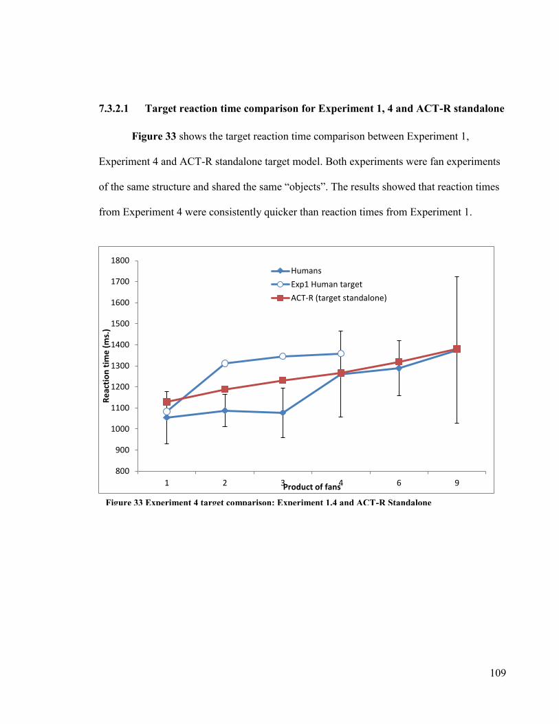
109

7.3.2.1 Target reaction time comparison for Experiment 1, 4 and ACT-R standalone

Figure 33 shows the target reaction time comparison between Experiment 1,

Experiment 4 and ACT-R standalone target model. Both experiments were fan experiments

of the same structure and shared the same “objects”. The results showed that reaction times

from Experiment 4 were consistently quicker than reaction times from Experiment 1.

800

900

1000

1100

1200

1300

1400

1500

1600

1700

1800

1 2 3 4 6 9

Re

acti

on

tim

e (

ms.

)

Product of fans

Humans

Exp1 Human target

ACT-R (target standalone)

Figure 33 Experiment 4 target comparison: Experiment 1,4 and ACT-R Standalone

(out(outlieroved)removed)simulation model

110

7.3.3 Foil Analysis

The foil reaction time analysis also compares human recognition foil results to two

fan models: 1) the standalone fan model where the fans were calculated based on the

propositions used in Experiment 4 alone. 2) The combined fan model where the fans were

calculated based on the propositions used in both Experiment 1 and 4. Figure 34 shows the

standalone ACT-R foil model reaction time analysis with all the data recorded from the

Experiment 4. Even with the inclusion of outliers, the results show 5 out of 6 predictions fell

within the 95% confidence intervals of the human data.

Figure 35 shows the standalone foil model reaction time analysis with the outliers

removed. There were 10 outlier removed out of 161 records. All of the outliers had a longer

reaction time than the mean, showing the anomalies were mostly due to hesitations. The

removal of the outliers had two practical effects: 1) it had slightly lowered the affected

means and 2) it had increased the resolutions for 95% confidence intervals; the affected

confidence intervals became smaller. With the outliers removed, the results show 4 out of 6

predictions fell within the 95% confidence intervals of the human data.

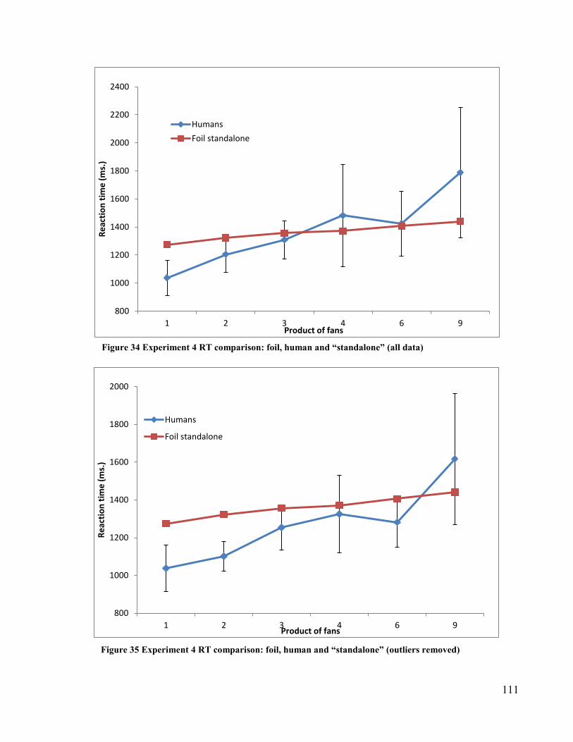
111

800

1000

1200

1400

1600

1800

2000

2200

2400

1 2 3 4 6 9

Re

acti

on

tim

e (

ms.

)

Product of fans

Humans

Foil standalone

800

1000

1200

1400

1600

1800

2000

1 2 3 4 6 9

Re

acti

on

tim

e (

ms.

)

Product of fans

Humans

Foil standalone

Figure 34 Experiment 4 RT comparison: foil, human and “standalone” (all data)

datadata)data)mulation model

Figure 35 Experiment 4 RT comparison: foil, human and “standalone” (outliers removed)

simulation model

112

The combined fan foil model for Experiment 4 used the datasets from Experiment 1

and 4 to calculate fan combinations for the analysis. Figure 36 shows the combined fan

model foil reaction time analysis with all the data. The results show 4 out of 6 foil

predictions fell within the 95% confidence intervals of the human data. Figure 37 shows the

combined fan model foil reaction time analysis with the outliers removed for the

Experiment 4. Again, there were 10 outlier records removed from 161 records. With the

outliers removed, the results show only 2 out of 6 predictions fell within the 95% confidence

intervals of the human data. A t-test identical to the one described above was performed on

the difference between each foil prediction and each actual reaction time (a two tailed,

paired t-test was performed). The average difference for the stand-alone model (outliers

removed) was -73 and an average difference for the combined model (outliers removed) was

-126 This difference was significant at P<0.001. Together with the target and foil RT

analyses, the standalone fan model with the outliers removed have consistently provided the

best fit model for Experiment 4.

113

800

1000

1200

1400

1600

1800

2000

2200

2400

2 4 6 8 12 18

Re

acti

on

tim

e (

ms.

)

Product of fans

Humans

Foil combined

800

1000

1200

1400

1600

1800

2000

2 4 6 8 12 18

Re

acti

on

tim

e (

ms.

)

Product of fans

Humans

Foil combined

Figure 36 Experiment 4 RT comparison: foil, human and “combined” (all data)

Figure 37 Experiment 4 RT comparison: foil, human and “combined” (outlier removed)

(out(outlieroved)removed)simulation model

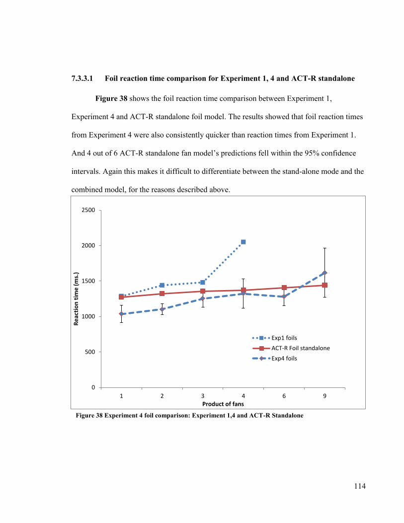
114

7.3.3.1 Foil reaction time comparison for Experiment 1, 4 and ACT-R standalone

Figure 38 shows the foil reaction time comparison between Experiment 1,

Experiment 4 and ACT-R standalone foil model. The results showed that foil reaction times

from Experiment 4 were also consistently quicker than reaction times from Experiment 1.

And 4 out of 6 ACT-R standalone fan model‟s predictions fell within the 95% confidence

intervals. Again this makes it difficult to differentiate between the stand-alone mode and the

combined model, for the reasons described above.

0

500

1000

1500

2000

2500

1 2 3 4 6 9

Re

acti

on

tim

e (

ms.

)

Product of fans

Exp1 foils

ACT-R Foil standalone

Exp4 foils

Figure 38 Experiment 4 foil comparison: Experiment 1,4 and ACT-R Standalone

(out(outlieroved)removed)simulation model

115

7.4 Discussion

Experiment 4 is an elapsed-time fan experiment. The aim is to investigate how the

passage of time might affect dataset boundaries. Similar to experiment 2, Experiment 4‟s

results can be interpreted by two possible fan modes. The standalone fan mode which

calculates its fan based upon Experiment 4‟s propositions alone. Or the combined fan mode

which calculates its fan based on the combined propositions of Experiment 1 and

Experiment 4 (since the objects in Experiment 4 had also appeared in Experiment 1). The

analysis will follow the line of inquiry described in Experiment 2.

Figures 29 to 36 show the reaction time comparisons for standalone and combined

modes for targets and foils. The conditions on the x-axis are the products of the fans of the

terms in the probes. The target and foil results show a good fit for the standalone model. All

standalone ACT-R target predictions fall within the 95% confidence intervals of human

performances but not quite for the combined fan model.

One interesting observation came from the comparison between human

performances in Experiment 1 and Experiment 4 (Figure 33, 38). A 2 x 4 ANOVA test

between Experiment 1 and Experiment 4 revealed that there were no significant interaction

between the experiments and fan factors, however, there is a significant main effect on

reaction time F(1,88) = 8.74, p <. 01. Experiment 4 reaction times were quicker (latencies

were smaller) than Experiment 1‟s results and the quicker results were not due to the fan

factors. The ANOVA summary is presented in Table 8.

116

Source of

Variation SS df MS F P-value F crit

Group 1296188 1 1296188 8.74 0.00 3.95

Columns 1592666 3 530889 3.58 0.02 2.71

Interaction 114708 3 38236 0.26 0.86 2.71

Within 13048376 88 148277

Total 16051938 95

Table 8 ANOVA test between Experiment 1 and 4

The results showed that the reaction times were much quicker in Experiment 4 than

in Experiment 1 and were consistent for each condition (except fan product of 1). This effect

might be due to a shift in the factors covered by the “I” parameter in the models? To test

this hypothesis Figure 33 has been re-graphed as Figure 33-A where the I parameter (the I

intercept) for ACT-R fan predictions was reduced by the difference based on “product of

fans” equals to 1 (the first data point where the performance difference is not influence by

fan) which is 30 ms. The results show a close match with human performance in Experiment

800

900

1000

1100

1200

1300

1400

1500

1600

1700

1800

1 2 3 4 6 9

Re

acti

on

tim

e (

ms.

)

Product of fans

Humans

Exp1 Human target

I adjusted

Figure 33a Experiment 4 target comparison: Experiment 1,4 and ACT-R Standalone

(out(outlieroved)removed)simulation model

117

4, showing the reaction time difference between Experiment 1 and 4 could be due to

learning that had an effect on parameter I but not caused by the fan effect. However, there

is an alternative to estimate the adjustment of the I parameter which is to use the average

difference of RT (150 ms.). The consequences of shifted I by -150 ms. will put the ACT-R

combined fan mode model to be an equal contender with the standalone mode. Therefore,

based on the ANOVA analysis alone it is inconclusive that Experiment 4 results reflect a

standalone or a combined fan model.

To further analyze the results, the RT scores for each subject were compared with

the model predictions for both fan modes (combined and standalone). This was done by

subtracting the human RT scores from each model‟s predicted RT scores for each trial. This

produced two difference scores for every trial, for every subject. The mean difference score

for the standalone model was -71 and the mean difference score for the combined model

was -185. Using a pairwise t-test we found that the difference scores for the combined and

standalone models were statistically significant (P<0.001) and the average for difference

scores for the stand alone model is also significantly smaller than the combined model

average difference - almost half of the standalone average difference (-71 compared to -

185). Therefore, based on the difference average analysis and the target and foil graphs

comparison the standalone fan model is proofing to be a better fit for Experiment 4.

A possible explanation for a consistent quicker reaction time difference for

Experiment 4 than Experiment 1 is that, there is learning and forgetting happening over the

passage of time. There is a consensus view in the literature that learning and forgetting

occurs in three stages (Kim & Ritter, 2015). In ACT-R‟s terms: stage 1 is the Acquisition

(declarative) learning and decay, stage 2 is Consolidation (declarative and procedural), and

stage 3 is Tuning (procedural). The likely explanation is that the fan effect which is mainly

associated with the declarative knowledge has decayed over the passage of time. However

118

there has been some residual procedural knowledge learned over the experiments and

procedural knowledge that is not affected by decay (Chong, 2004) and that, in practice

produced a smaller I parameter for reaction time over all conditions between Experiment 4

and 1.

7.5 Conclusion

Experiment 4 was designed to examine how the passage of time might affect the

scope of a fan model. The key findings are:

(1) The results of Experiment 4 were affected by the results of Experiment 1, human

reaction times was consistently quicker in Experiment 4 than in Experiment 1 for all

conditions except for the product fan of 1. An ANOVA test showed that there was no

significant interaction but there was a significant main effect. In addition, both standalone

and combined models have a negative average difference score (-71, -185) that shows a

consistent “learning” effect. One explanation for this learning effect is that subjects were

becoming quicker in reaction time from experiment to experiment. If parameter I

(representing perceptual and motor speed) became smaller due to some form of learning; it

would down-shift the reaction times as they appear in the results (see Figure 33-A). It is

also possible that a consolidation effect had occurred, making either spreading activation or

base level learning stronger and thus increasing retrieval speed. Since very little is published

on the effect of passage of time on fan effect, either explanation is possible.

(2) The results of the overall analysis show that the standalone model might be a better fit

for the human data, if this is true, this suggests that there is no implicit associated fan effect

from Experiment 1, i.e. from the fan perspective, what the participants had learned from

Experiment 1 did not affect what they learned in Experiment 4 possibly due to decay of

119

declarative knowledge. However, given the shifting of the I parameter analysis, the

standalone fan mode is not conclusive.

(3) The ACT-R fan model (standalone fan mode) continues to predict accurately; it behaves

like a regression model for the interrelated Experiment 1 and 4.

120

Experiment 5: Holographic Declarative Memory for Complex 8 Chapter:

Fan

The fan model is a fundamental building block for the complex fan paradigm. The

investigations of the fan model with the new Holographic Declarative Memory (HDM)

module are presented here. The purpose of Experiment 5 (simulation experiment) was to

apply the HDM model to the previous 4 experiments. This was used address the issue of the

viability of using the HDM module and to determine impact of detailed implementation on

Anderson‟s fan model and the complex fan model.

ACT-R is a widely used cognitive architecture that models many different aspects of

cognition. As an integrated architecture, ACT-R is a good choice for modelling complex

behavioural tasks. However, it has some limitations. Notably, the declarative memory

module is limited by its use of symbols to represent concepts or stimuli. The ACT-R

Declarative Memory system (DM) was designed for modelling the results of behavioural

experiments and as such presents certain limitations.

The Holographic DM, or HDM (Kelly, Kwok, & West, 2015) is a module that can

replace the DM model in Python ACT-R. HDM replaces the symbols with holographic

vectors. Holographic vectors retain the expressive power of symbols but provide a similarity

metric, allowing for shades of meaning, fault tolerance, and lossy compression. The purpose

of HDM is to enhance ACT-R’s ability to model lower level mind functions in associative

learning, learn over the long-term, and store large quantities of data. HDM provides a more

“realistic’ (in terms of scalability) memory module which is similar to the performance of

the human brain. The use of HDM might provide a better modelling platform for fan

modelling.

121

8.1 Holographic declarative memory module background

A holographic memory model was first proposed by Longuet-Higgins (Longuet-

Higgins, 1968), a holographic memory is a type of computational associative memory based

on the mathematics of holography. Memory is represented by high dimensional

mathematical vectors. The high dimensional vectors serve as an analogy of memory which

is constructed with a large number of neurons. With the introduction of high dimensional

vectors, one can formalize the descriptions for the basic mechanism for memory.

Cognitive models based on holographic memory can explain and predict a variety of

human memory phenomena, such as the serial position curve in free recall (Franklin &

Mewhort, 2013). Holographic memory has also been used to model analogical reasoning

(Plate, 2000; Eliasmith & Thagard, 2001) and how humans perform simple problem-solving

tasks such as playing rocks, paper, scissors ( Rutledge-Taylor et al., 2011). Knowledge in

SPAUN, the world’s largest functional brain model (Eliasmith, How to build a brain: A

neural architecture for biological cognition, 2013), is represented using holographic

memory. Holographic memory models have also been previously used to model fan effect.

Specifically, Dynamically Structured Holographic Memory (DSHM; Rutledge-Taylor et al.,

2014; Rutledge-Taylor, Pyke, West, & Lang, 2010) has been used to model two versions of

the fan effect task.

The HDM is based on DSHM. The difference between HDM and DSHM is that

HDM is a fully integrated Python ACT-R module. HDM is an optional memory module for

general ACT-R model development with Python ACT-R. To interface with ACT-R, HDM

commits to a particular way of encoding information and to a particular way of calculating

reaction times that are distinct from the DSHM model. In fact, the first successful

122

demonstration of HDM’s use is its replication of the results from the first fan experiment

(Anderson J. R., Retrieval of propositional information from long-term memory, 1974). The

theory and results have been published in 2015 ICCM proceedings (Kelly, Kwok, & West,

2015). The details of HDM’s techniques are included in Appendix G.

8.2 Model construction for fan and complex fan with HDM

To create the HDM model a model was first constructed in ACT-R using the default

DM module. Here it is important to note that the analytical fan models presented above,

following Anderson‟s mathematical or “analytical” model of the fan, makes slightly

different predictions from the same model constructed in ACT-R as a simulation. This is

because there are some minor differences between Anderson‟s mathematical model and how

spreading activation is implemented in the ACT-R architecture. In the analyses below the

analytical model used in the experiments above is referred to as the ACT-R model and the

ACT-R architecture simulation using the DM module is referred to as the DM model. To

create the HDM model results, the DM module was switched to the HDM module, so that

everything else in the model stayed the same. However, there were two ways to construct a

basic “recognition” fan simulation model with HDM.

8.2.1 HDM Request (query) based model

The first fan model uses a memory query production, which uses one of the terms in

a proposition as the basis for memory retrieval. This approach is how the original fan

analysis calculated the reaction times for foils. Statistically, the reaction time is the average

reaction time between the query productions from all the terms in a probe. This model is

referred to as the Hrq model.

8.2.2 HDM Resonance based model

123

The second fan model uses a memory resonance production, which models memory

retrieval as a direct chunk retrieval straight from long term memory. The retrieval

production is based on all the terms in a probe. And all terms provide spreading activation to

a memory chunk. The chunk that has the highest activation gets retrieved. This approach is

how the original fan analysis calculates the reaction times for targets. The reaction time is an

exponential function of the product of the fans. This model is referred to as the Hrs model.

8.2.3 HDM search model for Experiment 3

To model the search process in Experiment 3 an ACT-R simulation using the DM

module was constructed. Recall that Experiment 3 presented two analytical models,

corresponding to the fastest possible search and the longest possible search. The DM

simulation model would fall statistically in between as sometimes it would find the solution

quickly, and sometimes not. The HDM search model is the same model, only using the

HDM module instead of the DM module. The same ACT-R model was used in Experiment

3. The key differences are syntactic changes and the instantiation of the HDM memory

module. HDM is instantiated with the following parameters: retrieval, latency=0.63, N=256,

where retrieval, latency is the “F‟” parameter; and N = 256 is the vector size. The HDM

simulation models are documented in Appendix H.

8.3 HDM simulation and human performance comparisons

All of the analyses with HDM simulations were performed with the experiment data

with outliers removed. There were no foil analyses, since it was not clear how to directly

map Anderson‟s foil model to the HDM.

8.4 Experiment 1 and HDM Results

124

Figure 39 compares HDM request simulation (Hrq), the HDM resonance

simulation (Hrs) , ACT-R simulation (DM), ACT-R analytical model, and human

performance altogether. The x-axis is arranged in ascending order in terms of “product of

fans” as described in Experiment 1. All Hrq and Hrs predictions fell within the 95%

confidence intervals of human performance. And the root mean squared difference (RMSD)

for Hrq is 118.8 and 110.3 for Hrs. Both Hrq and Hrs are in excellent agreement with human

data for products fans 1 to 3, and Hrq begins to diverge slightly at the product fans of 4 and

yet all HDM predictions fell within the 95% confidence intervals of all human data. Overall,

the ACT-R analytical tracks closest to human data with a 26 RMSD.

8.4.1 Experiment 1 and HDM discussion and conclusion

800

900

1000

1100

1200

1300

1400

1500

1600

1 2 3 4

Re

acti

on

tim

e (

ms.

)

Product of fans

Exp1 Humans vs. HDM (request)

ACTR

Hrq simulation

Hrs simulation

DM simulation

Humans

Figure 39 Experiment 1 Comparison of human data with ACT-R (analytical), HDM and DM

simulations

125

HDM reaction time predictions are much quicker than the analytical model

predictions and the human data. However, both Hrq and Hrs simulation results fall within

the 95% confidence intervals of the human data. HDM simulations have independently

corroborated with the ACT-R‟s analytical model and human data.

8.5 Experiment 2 and HDM Results

HDM simulations are compared to Experiment 2‟s data with outliers removed.

8.5.1 HDM model combined mode reaction times

Figure 40 compares Experiment 2 human reaction times with the HDM combined

fan mode simulations (Hrq and Hrs), DM combined simulation, and ACT-R combined fan

mode. The x-axis is arranged in ascending order in terms of “product of fans” as described

in Experiment 2 in the combined fan mode. All HDM predictions fell within the 95%

confidence intervals of human performance. The combined fan root mean squared

difference (RMSD) for Hrq is 111 and the combined fan root mean squared difference

(RMSD) for Hrs is 108 showing that combined fan Hrs is a better fit model.

126

800

900

1000

1100

1200

1300

1400

1500

1600

2 3 4 6 9

Re

acti

on

tim

e (

ms.

)

Product of fans

Humans

ACT-R combined

Hrs combined

Hrq combined

DM simulation (combined)

Figure 40 Experiment 2 Comparison of human data with ACT-R, HDM and DM simulations

combined fan mode

127

8.5.2 HDM model standalone mode reaction times

Figure 41 compares Experiment human reaction times with the HDM 2 standalone

fan mode simulations (Hrq and Hrs)), DM standalone simulation, and ACT-R analytical

standalone fan mode. The x-axis is arranged in ascending order in terms of “product of fans”

in combined fan mode. All HDM predictions fall within the 95% confidence intervals of

human performance. The standalone fan root mean squared difference (RMSD) for Hrq is

117 and the standalone fan root mean squared difference (RMSD) for Hrs is 118 showing

that combined fan Hrs which has the smallest RMSD which is 108 is a better model.

800

900

1000

1100

1200

1300

1400

1500

1600

1 2 2 2 3

Re

acti

on

tim

e (

ms.

)

Product of fans

HumansACT-R stand aloneHrs stand aloneHrq stand aloneDM Simulation (standalone)

Figure 41 Experiment 2 Comparison of human data with ACT-R, HDM and DM simulations

standalone fan mode

128

8.5.3 Experiment 2 and HDM discussion and conclusion

The HDM simulation results (Hrq and Hrs) are consistent with the ACT-R analytical

predictions. Overall, HDM resonance combined fan model has the best RMSD; therefore it

is a better HDM model for Experiment 2. The HDM simulation results are providing

support to the previous conclusion that the combined fan mode is the appropriate fan mode

for Experiment 2.

8.6 Experiment 3 and HDM results

The complex fan HDM simulation is compared to Experiment 3‟s human data (with

outliers removed) and DM simulation. No foil data is being analyzed. Figure 42 shows the

reaction time results.

0

1000

2000

3000

4000

5000

6000

1-2-1 1-2-2 1-2-3 1-3-1 1-3-2 1-3-3 2-3-3 2-4-1 3-3-3

Re

acti

on

tim

e (

ms.

)

Fan combination

Humans

HDM

DM Simulation

Figure 42 Experiment 3 HDM and human data comparison

129

8.6.1 Experiment 3 and HDM discussion and conclusion

The HDM simulation for Experiment 3 is based on the ACT-R SCFM search

simulation model. The HDM model uses the same set of productions as in SCFM search

DM model. The difference is in the syntax of the memory request. RMSD between HDM

and humans is 1692 comparing this to PCFM and SCFM (no search), the RMSD for PCFM

and SCFM (basic) were 2216 and 1792 respectively. HDM has a smaller RMSD. HDM has

a smaller RMSD; it is acting like an improved SCFM basic model. One possible explanation

is that HDM retrievals did not require a lot of search time; i.e. not a lot of search time had

been added to the simulation. It could be that HDM retrievals were more accurate and less

noisy; it always got the target chunk at the first try.

130

8.7 Experiment 4 and HDM Results

HDM simulations are compared to Experiment 4‟s data with outliers removed.

8.7.1 HDM combined mode reaction time comparison

Figure 43 compares Experiment 4 human reaction times with the HDM combined

fan mode simulations (Hrq and Hrs), DM combined simulation, and ACT-R combined fan

model. The x-axis is arranged in ascending order in terms of “product of fans” in the

standalone fan mode. Only 2 HDM predictions fell within the 95% confidence intervals of

human performance. The combined fan root mean squared difference (RMSD) for Hrq is

119.6 and the combined fan root mean squared difference (RMSD) for Hrs is 123.4 showing

that combined fan mode is not a good fit.

800

900

1000

1100

1200

1300

1400

1500

1600

2 4 6 8 12

Re

acti

on

tim

e (

ms.

)

Product of fans (combined)

Humans

ACT-R combined

Hrs combined

Hrq combined

DM (combined)

Figure 43 Experiment 4 Comparison of human data with ACT-R, HDM and DM simulations

combined fan mode

131

8.7.2 HDM standalone mode reaction time comparison

Figure 44 compares Experiment 4 human reaction times with the HDM standalone

fan mode simulations (Hrq and Hrs) ), DM standalone simulation, and ACT-R standalone

fan mode. The x-axis is arranged in ascending order in terms of “product of fans” in

standalone fan mode. Three out of five predictions fell within the 95% confidence intervals

of human performance. The standalone fan root mean squared difference (RMSD) for Hrq

is 101 and the standalone fan root mean squared difference (RMSD) for Hrs is 94 showing

that standalone fan Hrs is a best model for Experiment 4.

800

900

1000

1100

1200

1300

1400

1500

1600

1 2 3 4 6

Re

acti

on

tim

e (

ms.

)

Product of fans (standalone)

Exp4 Target, Human vs. Hrs (standalone) Humans

ACT-R stand alone

Hrs stand alone

Hrq stand alone

DM (standalone)

Figure 44 Experiment 4 Comparison of human data with ACT-R, HDM and DM simulations

standalone fan mode

132

8.7.3 Experiment 4 and HDM discussion and conclusion

The HDM simulation results (Hrq and Hrs) are consistent with the ACT-R analytical

results. Based upon RMSDs, the HDM resonance standalone fan model has the smallest

RMSD for Experiment 4. Therefore, HDM Hrs standalone fan mode is the best model for

Experiment 4. Also it is apparent that there is some learning going on since all human data

at the low fan range has underperformed the model predictions. The learning effect in

Experiment 4 has been discussed in Experiment 4 (section7.4).

8.8 Conclusions

For modeling fan effect the resonance models (Hrs models) will work well with

target predictions as it is demonstrated with all the reaction time analyses in experiment 1, 2

and 4. The HDM resonance models consistently corroborated with all previous analyses.

The request/query production (Hrq models) is useful for foil modeling.

For Experiment 3, HDM was unable to produce better results than the SCFM search

analytical model. All HDM predictions were under-predicting the inference task. More work

is needed to enhance HDM to emulate human search heuristics.

Overall, all of the models did reasonably well. Although the HDM produced

different predictions there was no reason to conclude that the HDM did worse. In fact, it

arguably did better but realistically there was not sufficient evidence to distinguish between

the models. All of the models relied in some way on predicting the fan effect by estimating

the odds that the elements in the probe predicted the target. One of the advantages of the

HDM model is that this estimate falls out naturally from processing of the training chunks

into memory.

133

Overall, Anderson‟s fan model was not affected by the detailed implementation with

and an HDM module.

134

Conclusions and Summary 9 Chapter:

This set of five experiments, the associated models and tools, introduced a complex

fan paradigm for the extension of the ACT-R fan model. Overall this study shows that the

ACT-R fan model is a robust building block for complex fans.

The successful replication of fan effect results by the ACT-R fan analytical model in

Experiment 1 serves as a preliminary step for proposition learning and it has also provided a

reasonable assurance of the integrity of the design, the method, and the tools for this

research. It confirms that the even the sample size is relatively small but it is sufficient to

provide reasonable data; the design of the datasets used in these experiments is

counterbalanced - critical for fan models. It also show that the new tools developed for this

research are working together for successful analysis, validating the test and analysis

process for the rest of the complex fan experiments. Where dataset boundaries are

concerned, results from Experiments 1 and 2 show that the combined fan model is a better

assumption for the inference model construction for Experiment 3 – the ACT-R inference

test.

There are three key findings in the complex fan Experiment 3. (1) The ACT-R

spreading activation theory is a robust minimalist model which continues to predict un-

searched scenarios accurately in complex fan situations. ACT-R SCFM basic model plus

search time could provide a complete description for human data (within the 95%

confidence intervals). (2) Results from the search model show that the inference task is

achieved via a dual (serial) retrieval process and not by a single (parallel) retrieval process.

This shows that chunk structures are combined after retrievals unlike an organized mental

model. The relational inference reaction times are a combination of multiple spreading

135

activations and search time. (3) The search time is also fundamentally a fan function. In

Experiment 3, the search time is a function of object fan and container fan.

In the investigation into the effect of passage of time in fan effect, results from

Experiment 4 show that there is a learning effect between Experiment 1 and 4 even though

the analysis favors the standalone fan mode showing fan effect might not be extend with the

passage of time but the analysis is not conclusive.

This study concluded with an alternative way of implementing fan models using a

holographic memory system. The results showed all the fan models continue to provide a

reasonable account for the human results indicating that the power of the fan model comes

from the conceptual structure of the theory and not the specific ways in which it is

implemented. All of the models have some deviations from the human data suggesting that

all of the models are close descriptions but none is perfect. Overall, the introduction of the

HDM module appears to have no significant impact on the fan model.

The following are areas that need further research:

(1) The current foil theory is inadequate in explaining the high fan results. Alternate

approach based on heuristic rather than statistical reasoning may be explored.

(2) The factors and causes for the improved performance or “learning” with the passage of

time need to be studied and identified.

(3) An alternate model exists for the query production in complex fan, the SCFM1 model

described in Appendix D.2. The query production time can be modelled as a function of the

fan of the cue plus the fans from the retrieved chunk rather than just the function of the

query cue.

(4) Currently HDM only provide two kinds of memory retrieval productions: a query or a

resonance. Foil is simply modelled as a failed “resonance” request or a failed query request.

136

So, HDM is agnostic for a “foil” theory. By the same reason, HDM is also agnostic in terms

of memory search strategies.

(5) The sample size used in the experiments was small; it is probably not sufficient to

satisfactorily build a general theory. So the future work is to scale up all the experiments to

the appropriate sample size.

This research has extended ACT-R fan model to explain complex fan situations. The

models and analyses from the five experiments, based on zero parameter, have shown the

robustness and versatility of ACT-R and the fan model. With the integration of HDM and

the complex fan tools, this research has provided an expanded ACT-R platform for higher

cognitive task research and has successfully provided a modular explanation of an inference

task based on complex fan analysis.

.

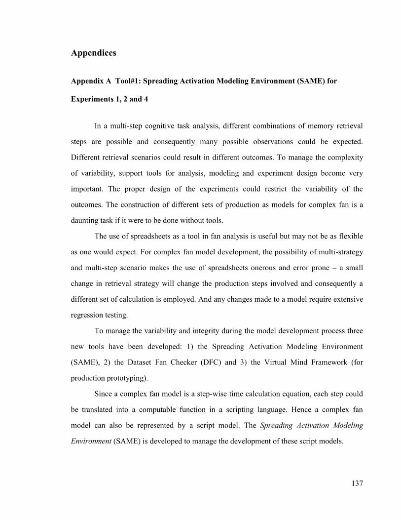
137

Appendices

Appendix A Tool#1: Spreading Activation Modeling Environment (SAME) for

Experiments 1, 2 and 4

In a multi-step cognitive task analysis, different combinations of memory retrieval

steps are possible and consequently many possible observations could be expected.

Different retrieval scenarios could result in different outcomes. To manage the complexity

of variability, support tools for analysis, modeling and experiment design become very

important. The proper design of the experiments could restrict the variability of the

outcomes. The construction of different sets of production as models for complex fan is a

daunting task if it were to be done without tools.

The use of spreadsheets as a tool in fan analysis is useful but may not be as flexible

as one would expect. For complex fan model development, the possibility of multi-strategy

and multi-step scenario makes the use of spreadsheets onerous and error prone – a small

change in retrieval strategy will change the production steps involved and consequently a

different set of calculation is employed. And any changes made to a model require extensive

regression testing.

To manage the variability and integrity during the model development process three

new tools have been developed: 1) the Spreading Activation Modeling Environment

(SAME), 2) the Dataset Fan Checker (DFC) and 3) the Virtual Mind Framework (for

production prototyping).

Since a complex fan model is a step-wise time calculation equation, each step could

be translated into a computable function in a scripting language. Hence a complex fan

model can also be represented by a script model. The Spreading Activation Modeling

Environment (SAME) is developed to manage the development of these script models.

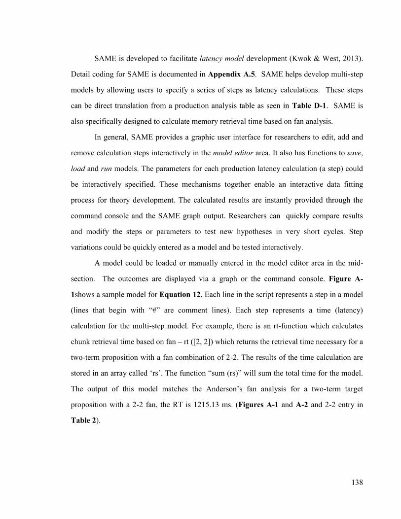
138

SAME is developed to facilitate latency model development (Kwok & West, 2013).

Detail coding for SAME is documented in Appendix A.5. SAME helps develop multi-step

models by allowing users to specify a series of steps as latency calculations. These steps

can be direct translation from a production analysis table as seen in Table D-1. SAME is

also specifically designed to calculate memory retrieval time based on fan analysis.

In general, SAME provides a graphic user interface for researchers to edit, add and

remove calculation steps interactively in the model editor area. It also has functions to save,

load and run models. The parameters for each production latency calculation (a step) could

be interactively specified. These mechanisms together enable an interactive data fitting

process for theory development. The calculated results are instantly provided through the

command console and the SAME graph output. Researchers can quickly compare results

and modify the steps or parameters to test new hypotheses in very short cycles. Step

variations could be quickly entered as a model and be tested interactively.

A model could be loaded or manually entered in the model editor area in the mid-

section. The outcomes are displayed via a graph or the command console. Figure A-

1shows a sample model for Equation 12. Each line in the script represents a step in a model

(lines that begin with “#” are comment lines). Each step represents a time (latency)

calculation for the multi-step model. For example, there is an rt-function which calculates

chunk retrieval time based on fan – rt ([2, 2]) which returns the retrieval time necessary for a

two-term proposition with a fan combination of 2-2. The results of the time calculation are

stored in an array called „rs‟. The function “sum (rs)” will sum the total time for the model.

The output of this model matches the Anderson‟s fan analysis for a two-term target

proposition with a 2-2 fan, the RT is 1215.13 ms. (Figures A-1 and A-2 and 2-2 entry in

Table 2).

139

Figure A-1 SAME Sample Model for a Target with Fan 2-2

Figure A-2 SAME Sample Model Output for a Target with Fan 2-2

140

SAME also provides an interactive graphical output for users to compare results.

Figure A-3 shows a comparison between Anderson‟s 1974 target data to his target analysis

based on ACT-R (foils are not included). The vertical axis is RT from the recognition

experiment in ms, and the horizontal axis is the total fan in a probe. Red represents human

performance data (Table 1) and green are ACT-R calculated data (data summarized in

Table 2). This example demonstrates the accuracy of SAME - it is able to reproduce

Anderson‟s fan experiment analysis.

Figure A-3 SAME Sample Graph Output

141

SAME provides a set of ACT-R based time calculation functions to support fan and

complex fan analysis. To build a complex fan RT model, the first step is to complete a high-

level task analysis by identifying all the atomic-steps or the productions required for the

memory task. Once the high-level analysis is completed, each step can be translated into a

specific function call in a SAME model. Alternatively, if the RT calculation can be

expressed in an equation, each term in the equation can be translated into a function call in a

SAME model.

SAME does not replace the use of spreadsheet tools. Spreadsheet tools continue to

be useful in data integration, preparations, and presentation and also for fast prototyping that

does not require iterative development cycles. However, SAME can complement the

spreadsheet tools by cross-checking results especially for complex model calculations. This

is one of SAME‟s applications in this dissertation.

A.1 Analytical Models for Experiment 3 using SAME

The application of SAME is to build the serial and parallel complex fan latency

models described by Equations 14 to Equation 17.

As an illustration, these equations are applied to the production analysis of the

relational inference mechanism previously described.

The test subject is assumed to have learned two propositions: “A is B” and “B is C”.

A probe “A is C” is presented to the subject for a judgment if the probe is true. In the

present example, the fan of “A” and “C” are equal to1 and the fan of “B” is 2, the SAME

SCFM RT calculation could be specified as described in Figure A-4 - a SAME model, and

Figure A-5 shows the SAME output from the command console. The predicted RT from

the SAME calculation is 1483 ms, which corresponds exactly to the sample calculation in

the previous section.

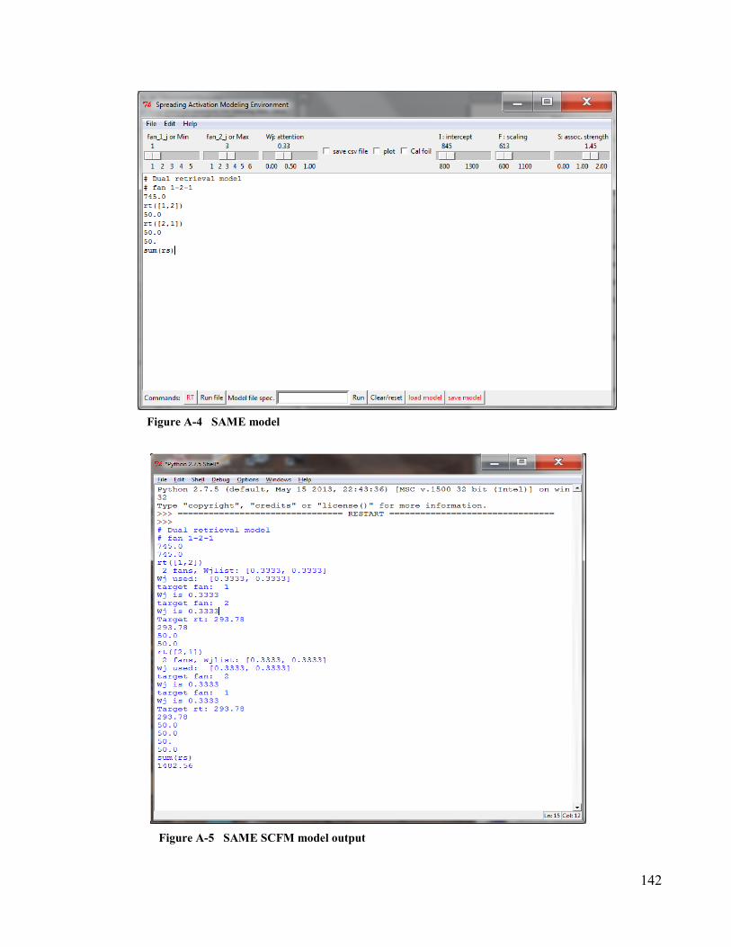
142

Figure A-5 SAME SCFM model output

Figure A-4 SAME model

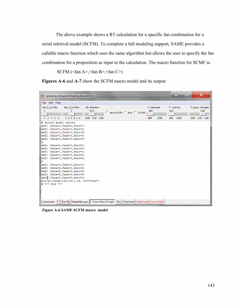
143

The above example shows a RT calculation for a specific fan combination for a

serial retrieval model (SCFM). To complete a full modeling support, SAME provides a

callable macro function which uses the same algorithm but allows the user to specify the fan

combination for a proposition as input to the calculation. The macro function for SCMF is:

SCFM (<fan A>,<fan B>,<fan C>)

Figures A-6 and A-7 show the SCFM macro model and its output:

Figure A-6 SAME SCFM macro model

144

Figure A-7 SAME SCFM macro output

145

A.2 SAME and the Three-term Fan Foil

Another application of SAME concerns the analysis of the three-term fan experiment

(West & Pyke, 2010). The three-term fan experiment is a natural extension of the 1974 two-

term fan experiment. The experiment has extended the range of the total fan from the

original 6 to 12. The reported ACT-R target predictions continue to track closely with

human performance in the extended range even with an additional term. However, the foil

results are very different from predictions. There are large differences between prediction

and experimental data for foils at the higher fans. Since foil calculations are a part of fan

analysis, this result could have bearings for complex fan. Therefore, it is important that

these discrepancies be investigated.

Investigating the foil discrepancy requires a cycle of: theorizing, adjusting

parameters, calculating RT and comparing model outputs with experimental data. The

process is slow moving with traditional tools but, with the development of SAME, the cycle

may be made much faster. SAME facilitates Fan Effect RT calculations by providing an

interactive graphical user interface to inject interactions in the steps of changing parameter

values, calculation and comparisons.

The investigation of three-term foils begins with the definition of the discrepancy.

Figure A-8 shows the SAME output comparing ACT-R predictions (in red) with the

experimental results (in green).

146

Figure A-8 Three Term Fan Foil RT Comparison, prediction (red), experimental results (green)

The x-axis represents the total fan in a probe and the y-axis is RT (ms). Within the

lower fan range, from 3 to 6, the difference between the theoretical value and the human

performance appears to be a constant value. But in the range from 6 to 12, the difference

between the model and the actual data has changed from a constant to an exponential

function.

West, Pyke et al. provided a model to fit the results, by introducing the latency

exponential parameter ( f ), part of ACT-R 6.0, where Equation 9 is modified by f :

)

By setting f = 3, and increase F from 613 to 2000 they obtained a good fit to the

experimental foil data. However, the introduction of the latency exponential parameter

147

needs a rational justification. The initial speculation by West et al is that the f parameter

represents an interference effect and suggested more research to confirm this. However, the

question is: is there an alternative that is more compatible with the standard fan analysis?

Can standard fan analysis model the foil observations without the addition of a new

parameter? What would a zero-parameter model look like? This is an opportunity to

demonstrate the flexble application of SAME.

A.3 Parameter Analysis for Three-term Foils

To build a new model for the three-term foil data is to apply the standard fan

equations (Equation 9). This does not require the introduction of a new parameter. And

the model will use the same values for the parameters that are set by previous findings such

as: I = 845 ms, where I is the intercept parameter which estimates the probe encoding and

other necessary productions, F’ is the scaling parameter that includes the base level

estimate, F’= 613, S=1.45, S is the associative strength estimate for the data set – which is

related to the data size. The values of the parameters was adjusted to the experimental

differences such as the design of the test data set. The intercept parameter I was adjusted to

reflect the encoding of three terms rather than two, the test data set size was increased with a

minor adjustment for parameter S. Finally it was observed that the prediction gap changed

as the total number of fan increased, suggesting that the F parameter could be a function of

total fan rather than a constant difference, as previously assumed.

To describe the relationship between F and total fan for RT, an exponential function

was used to approximate the adjusted F values. The adjusted F values for total fan(tf) from 3

to 6 is 900, and for total fan 9, F is 1300, the value 1300 comes from 900 plus the difference

between the two data points for fan 6 and fan 9 (400), and using the similar calculation for

total fan 12, F is 1650.

Figure A-9 shows the exponential calculation that describes the function:

148

The final adjustments of the parameters for three-term foil data are:

I = 950 ms. to account for the third term encoding.

F’ , the scaling parameter is a function of fan

F’= 900 ms. for fan from 3 to 6

F’= 1300 ms. for fan = 9

F’= 1650 ms. for fan = 12

S is the associative strength estimate for the data set,

S=1.5

y = 664.69e0.0729x R² = 0.9

0

200

400

600

800

1000

1200

1400

1600

1800

0 2 4 6 8 10 12 14

F p

aram

ete

r

Fan size

Figure A-9 F Parameter as a Function of Total Fan

149

A.4 SAME Model and Graph Output for Three-term Foils

Figure A-10 shows the SAME model with the adjusted parameters for fitting the foil

data performance. Based on empirical data and using SAME to adjust three parameters I, S

and F, a SAME model was built to describe the three-term foil data. This demonstrates the

possible usefulness of SAME in interactive RT model development. Figure A-11 shows

that the output of the model is a very close fit to the human data.

Figure A-10 A SAME Three-Term Fan Foil Model

150

Figure A-11 SAME Three-Term Fan Foil Model Output (red) and Human

Performance (green)

(ms)

151

A.5 Spreading Activation Modeling Environment (SAME) code

# Spreading Activation Modeling Environment

# Author: Kam Kwok, copyright 2012, 2013, 2014

# Complex and Classic Fan Effect RT calculations

# Version 1.0

# Functions supporting complex fan modeling: SCFM, and PCFM, rt, RT2

#

# This program requires numpy, math, matplotlib modules.

# All parameters are set from GUI except Bi.

from Tkinter import *

import tkMessageBox

import tkFileDialog

import math

import pylab # from matplotlib pkg

### global variables and utilities section

# for a 2/3 term proposition

Wj=0.333

# data set size related s = log(size); size = 26 for 1.45

S=1.45

# data set is counter-balanced therefore baselevel is a constant, estimate is absorbed into F

#

Bi=0

# I = encoding +productions (mem retrieval,judgment etc.) +motor movement; in ms.

I = 845

rtprdtime=100

# complex fan new intercept

Ic= I - rtprdtime

# empirical based estimate

F= 613

T=True

probe=[]

log=[]

#file lines/ program counter function for modeling, this support goto command

rs = []

# used by tkdialog; set to model filetype = .mdl

myFormats = [

('Model file', '*.mdl')

## ('Windows Bitmap','*.bmp'),

## ('Portable Network Graphics','*.png'),

## ('JPEG / JFIF','*.jpg'),

]

152

def defaults():

global Bi, rs

try:

sS.set(1.45)

sF.set (613)

sI.set (845)

Win.set (0.333)

Bi = 0

rs=[]

except:

print "Cannot set widget var!!!"

# used by models to set w,i,f, and s

# usage: in model - e.g. set_p(w=0.5)

def set_p(w=Wj,i=I,f=F,s=S, b=Bi):

global Bi,Wj

try:

sS.set(s)

sF.set (f)

sI.set (i)

Win.set (w)

Wj=w

Bi=b

print "set Wj", Wj

except:

print "Cannot set widget var!!!"

# used by models to output a message with a new window

# usage in model: e.g. msg('window label', 'message')

def msg(mlab,msg):

tkMessageBox.showinfo(mlab, msg)

#***

# run a text file model: a model is defined in a text file

# input: a text file name (a string)

# returns/output: the combined results of the modeling steps

# used by:

#++++++> experimental section <++++++++++++++++

def parseline (l):

if '#' in l:

print l, #print comment

else:

try:

153

print l

s1 = eval(l) # 'i' contains an expression not a statement

print s1

return s1

except:

print "Cannot evaluate input line!!!"

return 0

def run_model(f):

# results (rs) list whihc can be indexed as input to model steps

global rs

rs=[]

s1=0

if isinstance(f,file):

#run object

## try:

for i in f.readlines():

log.append(i) # lines os a global list the stores all file iines

if '#' in i:

print i, #print comment

else:

if len(i) > 4:

print i

s1 = eval(i) # 'i' contains an expression not a statement

if isinstance(s1, float): rs.append(s1)

print s1

s1=0

f.close()

## except:

## msg('Interpreter','command not found!!!')

else:

#run name, assume f is a string

try:

fi = open(f, 'r')

for i in fi.readlines():

log.append(i)

if '#' in i:

print i, #print comment

else:

if len(i) > 4:

print i

s1 = eval(i) # 'i' contains an expression not a statement

if isinstance(s1, float): rs.append(s1)

print s1

s1=0

154

fi.close()

except:

msg('fn_Interpreter','command not found!!!')

#++++++> experimental section <++++++++++++++++

def run_model_fn(f):

rs=[]

try:

fi = open(f, 'r')

for i in fi.readlines():

i = i.strip()

if i == "": continue

log.append(i)

if '#' in i:

print i, #print comment

else:

if len(i) > 4:

print i

s1 = eval(i) # 'i' contains an expression not a statement

if isinstance(s1, float): rs.append(s1)

print s1

s1=0

fi.close()

except:

msg('Interpreter','command not found!!!')

# file dialog provides a file object

def run_model_obj(f):

rs=[]

try:

data = f.readlines()

f.close()

for i in data:

i = i.strip()

if i == "": continue

log.append(i) # lines os a global list the stores all file iines

if '#' in i:

print i, #print comment

else:

if len(i) > 4:

print i

s1 = eval(i) # 'i' contains an expression not a statement

## if not isinstance(s1, str): rs.append(s1)

if isinstance(s1, float): rs.append(s1)

print s1

s1=0

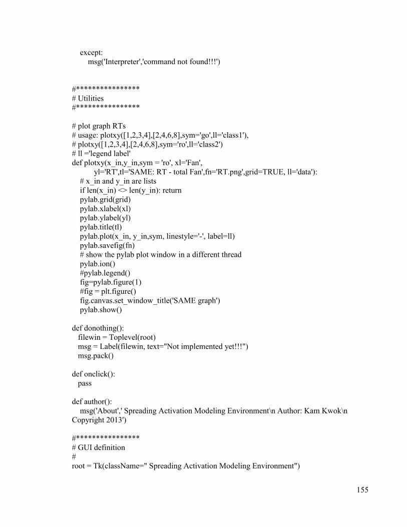
155

except:

msg('Interpreter','command not found!!!')

#****************

# Utilities

#****************

# plot graph RTs

# usage: plotxy([1,2,3,4],[2,4,6,8],sym='go',ll='class1'),

# plotxy([1,2,3,4],[2,4,6,8],sym='ro',ll='class2')

# ll ='legend label'

def plotxy(x_in,y_in,sym = 'ro', xl='Fan',

yl='RT',tl='SAME: RT - total Fan',fn='RT.png',grid=TRUE, ll='data'):

# x_in and y_in are lists

if len(x_in) <> len(y_in): return

pylab.grid(grid)

pylab.xlabel(xl)

pylab.ylabel(yl)

pylab.title(tl)

pylab.plot(x_in, y_in,sym, linestyle='-', label=ll)

pylab.savefig(fn)

# show the pylab plot window in a different thread

pylab.ion()

#pylab.legend()

fig=pylab.figure(1)

#fig = plt.figure()

fig.canvas.set_window_title('SAME graph')

pylab.show()

def donothing():

filewin = Toplevel(root)

msg = Label(filewin, text="Not implemented yet!!!")

msg.pack()

def onclick():

pass

def author():

msg('About',' Spreading Activation Modeling Environment\n Author: Kam Kwok\n

Copyright 2013')

#****************

# GUI definition

#

root = Tk(className=" Spreading Activation Modeling Environment")

156

master = root

menubar = Menu(root)

filemenu = Menu(menubar, tearoff=0)

filemenu.add_command(label="New", command=donothing)

filemenu.add_command(label="Open", command=donothing)

filemenu.add_command(label="Save", command=donothing)

filemenu.add_command(label="Save as...", command=donothing)

filemenu.add_command(label="Close", command=donothing)

filemenu.add_separator()

filemenu.add_command(label="Exit", command=root.destroy)

menubar.add_cascade(label="File", menu=filemenu)

editmenu = Menu(menubar, tearoff=0)

editmenu.add_command(label="Undo", command=donothing)

editmenu.add_separator()

editmenu.add_command(label="Cut", command=donothing)

editmenu.add_command(label="Copy", command=donothing)

editmenu.add_command(label="Paste", command=donothing)

editmenu.add_command(label="Delete", command=donothing)

editmenu.add_command(label="Select All", command=donothing)

menubar.add_cascade(label="Edit", menu=editmenu)

helpmenu = Menu(menubar, tearoff=0)

helpmenu.add_command(label="Help Index", command=donothing)

helpmenu.add_command(label="About...", command=author)

menubar.add_cascade(label="Help", menu=helpmenu)

## UI definition

frame = Frame(master)

frame.pack()

sS=DoubleVar(value = 1.45)

S = Scale(frame, label = "S: assoc. strength", variable=sS,

from_=1, to=2, tickinterval=1, resolution=0.01, orient='horizontal')

S.pack(side=RIGHT)

sF=IntVar(value = 613)

F = Scale(frame, label = "F : scaling", variable=sF,

from_=600, to=1500, tickinterval=500, resolution=1, orient='horizontal')

F.pack(side=RIGHT)

sI=IntVar(value = 845)

I = Scale(frame, label = "I : intercept", variable=sI,

from_=800, to=1500, tickinterval=500, resolution=1, orient='horizontal')

I.pack(side=RIGHT)

aw = IntVar(value = 0)

opt_aw = Checkbutton(frame, text = "Cal foil", variable=aw)

157

opt_aw.pack(side=RIGHT)

vplot = IntVar(value = 0)

opt_plot = Checkbutton(frame, text = "plot", variable=vplot)

opt_plot.pack(side=RIGHT)

logstatus = IntVar(value = 0)

opt_logstatus = Checkbutton(frame, text = "save csv file", variable=logstatus)

opt_logstatus.pack(side=RIGHT)

Win=DoubleVar(value = 0.3333)

W = Scale(frame, label = "Wj: attention", variable=Win,

from_=0, to=1, tickinterval=0.5, resolution=0.01, orient='horizontal')

W.pack(side=RIGHT)

f2=IntVar(value = 3)

fan2i = Scale(frame, label = "fan_2_j or Max", variable=f2,

from_=1, to=6, tickinterval=1, orient='horizontal')

fan2i.pack(side=RIGHT)

f1=IntVar(value = 1)

fan1i = Scale(frame, label = "fan_1_j or Min", variable=f1,

from_=1, to=5, tickinterval=1.0, orient='horizontal')

fan1i.pack(side=RIGHT)

# GUI event handlers

def cal_rt():

if aw.get():

print "1999 published value for [1,3] foil: 1306.66 ms."

foil = RT([f1.get(),f2.get()], Wj=Win.get(),

S=sS.get(), Bi=0, I=sI.get(),

F=sF.get(), target=False )

else:

print "1999 published value for [2,2] target: 1215.13 ms."

rt = RT([f1.get(),f2.get()], Wj=Win.get(),

S=sS.get(), Bi=0, I=sI.get(),

F=sF.get())

# for testing new routines using RT-btn

def calibrate_RT_btn():

probe = [2,2]

print "1999 published value for [2,2] target: 1215.13 ms."

RT(probe , Wj=Win.get(),

S=sS.get(), Bi=0, I=sI.get(),

F=sF.get() )

probe = [1,3]

print "1999 published value for [1,3] foil: 1306.66 ms."

RT(probe , Wj=Win.get(),

S=sS.get(), Bi=0, I=sI.get(),

F=sF.get(), target=False )

def run_orderlist():

158

# 1. constructing an input list of [[1,1], [1,2],[1,3], [2,1]...] from the

# sliders

inlist =[]

# creates an input list based on two slider values

for x in range(f1.get(),f2.get()+1):

for y in range(f1.get(),f2.get()+1):

inlist.append([x,y])

# run RT on input list and GUI based parameters

doList (inlist, Win.get(),sS.get(),

0,sI.get(),

sF.get())

def newlist():

inlist =[]

# creates an input list based on two slider values

for x in range(f1.get(),f2.get()+1):

for y in range(f1.get(),f2.get()+1):

inlist.append([x,y])

return inlist

#run command - run model in the text box

def run_file():

file = tkFileDialog.askopenfile(parent=root,mode='rb',title='Choose a file')

if file != None:

E1.insert(0,file.name)

run_model(file)

frame2 = Frame(master)

frame2.pack(fill=BOTH)

text = Text(frame2)

text.pack(fill=BOTH)

L2 = Label(frame2, text="Commands: ")

L2.pack( side = LEFT)

b_cal = Button(frame2, text="RT", fg="red", command=cal_rt)

b_cal.pack(side=LEFT)

b_plot = Button(frame2, text="Run file", command=run_file)

b_plot.pack(side=LEFT)

L1 = Label(frame2, text="Model file spec.")

L1.pack( side = LEFT)

content = StringVar()

E1 = Entry(frame2, bd =5,textvariable=content)

E1.pack(side = LEFT)

#run command: run model in a file (file object)

def run_text():

global rs

rs=[]

s1=0

159

## try:

contents = text.get(0.0, END)

for i in contents.split('\n'):

i = i.strip()

if i == "": continue

log.append(i) # lines os a global list the stores all file iines

if '#' in i:

print i #print comment

else:

if len(i) > 0:

print i

s1 = eval(i) # 'i' contains an expression not a statement

if isinstance(s1, float): rs.append(s1)

print s1

s1=0

## except:

## msg('run_textbox:','Error in script!')

##

##def run_text():

## global rs

## rs=[]

## s1=0

## try:

## contents = text.get(0.0, END)

## for i in contents.split('\n'):

## i = i.strip()

## if i == "": continue

## log.append(i) # lines os a global list the stores all file iines

## if '#' in i:

## print i #print comment

## else:

## if len(i) > 0:

## print i

## s1 = eval(i) # 'i' contains an expression not a statement

## if isinstance(s1, float): rs.append(s1)

## print s1

## s1=0

## except:

## msg('run_textbox:','Error in script!')

# clear text and entry and reset all sliders

def clear():

text.delete(1.0, END)

E1.delete (0,END)

defaults()

## calibrate_RT_btn()

160

# button event handlers

def loadf():

f = tkFileDialog.askopenfile(parent=root,mode='rb',title='Choose a file')

if f != None:

#E1 is the Entry/textbox

E1.delete (0,END)

E1.insert(0,f.name)

text.delete(1.0, END)

text.insert(INSERT, f.read())

f.close

def saveas():

fn = tkFileDialog.asksaveasfilename(parent=root,filetypes=myFormats ,title="Save the

image as...")

if len(fn) >0:

f = open(fn,'w')

f.write(text.get(0.0, END))

f.close

print 'File %s is saved.' % fn

else:

print 'zero file name! file not saved'

##b_exec = Button(frame2, text="Run", command=run_file) # run_model_fn

b_exec = Button(frame2, text="Run", command=run_text) # call handler - run_model_text

box

b_exec.pack(side=LEFT)

b_clear = Button(frame2, text="Clear/reset", command=clear)

b_clear.pack(side=LEFT)

b_load = Button(frame2, text="load model", fg="red", command=loadf)

b_load.pack(side=LEFT)

b_save = Button(frame2, text="save model", fg="red", command=saveas)

b_save.pack(side=LEFT)

#**************** GUI ends *************

#**************** memory retrieval time

(rt)**************************************

# Function: rt calculations; RT = target, single or foil

# input: a list of fanouts of a probe e.g. [1,2]

# returns/output: a rt, parameter target =False denotes foil calculation

# used by:

# used by models to calculate target;probe is a list of fanouts; foil:(set target=False), and

single fan response time

# usage: in model - e.g. rt([2,2], target=False)

def rt(probe, Wj=Win.get(), Wjl=[],S=sS.get(),Bi=Bi,F = sF.get(), target=TRUE):

sum_wj_sji =0

161

pl= len(probe) # probe length = number of fanout in the list

if len(Wjl) == 0:

if pl == 2:

# Wj list based on GUI input

Wjlist=[Wj]*pl

print " 2 fans, Wjlist:",Wjlist

if pl > 2 :

Wj = 1/float(pl) # calculate Wj when fan is > 2

#create Wj list

Wjlist=[Wj]*pl

if pl==1:

Wjlist=Wj

else:

Wjlist = Wjl

print "Wj used: ", Wjlist

if pl >1: # for multiple fan target or foil; else for single fan recall

if target: # calculate target

#for x, y in map(None, a, b):

for f,w in map(None,probe,Wjlist):

print "target fan: ",f

ln_fan_j = math.log(f)

Sji = S-ln_fan_j

print "Wj is",w

sum_wj_sji = sum_wj_sji + (w*Sji)

Ai = Bi+sum_wj_sji

rt = F*math.exp(-Ai)

print "Target rt: %4.2f " % rt

else: # foil calculation

rt_foils = []

for f,w in map(None,probe,Wjlist):

print "foil fan: ",f

ln_fan_j = math.log(f)

Sji = S-ln_fan_j

print "Wj is",w

sum_wj_sji = w*Sji # set sum to individual Sji

Ai = Bi+sum_wj_sji

rtf = F*math.exp(-Ai)

rt_foils.append(rtf) # a list of rt(fan)

foil_rt = sum(rt_foils)/len(rt_foils) # foil = average singles

rt = foil_rt

print "Foil rt: %4.2f " % rt

else: #single rt calculation

f = probe[0]

ln_fan_j = math.log(f)

print "Wj is",Wj

Sji = S-ln_fan_j

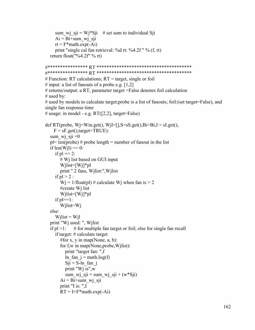
162

sum_wj_sji = Wj*Sji # set sum to individual Sji

Ai = Bi+sum_wj_sji

rt = F*math.exp(-Ai)

print "single cal fan retrieval: %d rt: %4.2f " % (f, rt)

return float("%4.2f" % rt)

#**************** RT **************************************

#**************** RT **************************************

# Function: RT calculations; RT = target, single or foil

# input: a list of fanouts of a probe e.g. [1,2]

# returns/output: a RT, parameter target =False denotes foil calculation

# used by:

# used by models to calculate target;probe is a list of fanouts; foil:(set target=False), and

single fan response time

# usage: in model - e.g. RT([2,2], target=False)

def RT(probe, Wj=Win.get(), Wjl=[],S=sS.get(),Bi=Bi,I = sI.get(),

F = sF.get(),target=TRUE):

sum_wj_sji =0

pl= len(probe) # probe length = number of fanout in the list

if len(Wjl) == 0:

if pl == 2:

# Wj list based on GUI input

Wjlist=[Wj]*pl

print " 2 fans, Wjlist:",Wjlist

if pl > 2 :

Wj = 1/float(pl) # calculate Wj when fan is > 2

#create Wj list

Wjlist=[Wj]*pl

if pl==1:

Wjlist=Wj

else:

Wjlist = Wjl

print "Wj used: ", Wjlist

if pl >1: # for multiple fan target or foil; else for single fan recall

if target: # calculate target

#for x, y in map(None, a, b):

for f,w in map(None,probe,Wjlist):

print "target fan: ",f

ln_fan_j = math.log(f)

Sji = S-ln_fan_j

print "Wj is",w

sum_wj_sji = sum_wj_sji + (w*Sji)

Ai = Bi+sum_wj_sji

print "I is: ",I

RT = I+F*math.exp(-Ai)

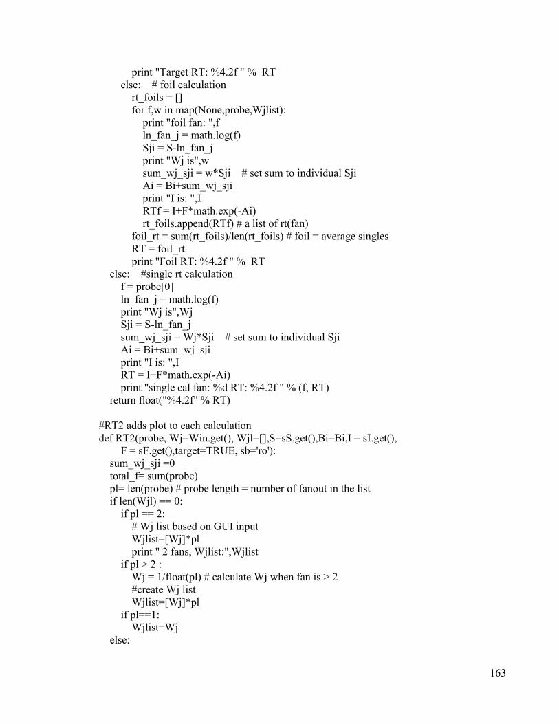
163

print "Target RT: %4.2f " % RT

else: # foil calculation

rt_foils = []

for f,w in map(None,probe,Wjlist):

print "foil fan: ",f

ln_fan_j = math.log(f)

Sji = S-ln_fan_j

print "Wj is",w

sum_wj_sji = w*Sji # set sum to individual Sji

Ai = Bi+sum_wj_sji

print "I is: ",I

RTf = I+F*math.exp(-Ai)

rt_foils.append(RTf) # a list of rt(fan)

foil_rt = sum(rt_foils)/len(rt_foils) # foil = average singles

RT = foil_rt

print "Foil RT: %4.2f " % RT

else: #single rt calculation

f = probe[0]

ln_fan_j = math.log(f)

print "Wj is",Wj

Sji = S-ln_fan_j

sum_wj_sji = Wj*Sji # set sum to individual Sji

Ai = Bi+sum_wj_sji

print "I is: ",I

RT = I+F*math.exp(-Ai)

print "single cal fan: %d RT: %4.2f " % (f, RT)

return float("%4.2f" % RT)

#RT2 adds plot to each calculation

def RT2(probe, Wj=Win.get(), Wjl=[],S=sS.get(),Bi=Bi,I = sI.get(),

F = sF.get(),target=TRUE, sb='ro'):

sum_wj_sji =0

total_f= sum(probe)

pl= len(probe) # probe length = number of fanout in the list

if len(Wjl) == 0:

if pl == 2:

# Wj list based on GUI input

Wjlist=[Wj]*pl

print " 2 fans, Wjlist:",Wjlist

if pl > 2 :

Wj = 1/float(pl) # calculate Wj when fan is > 2

#create Wj list

Wjlist=[Wj]*pl

if pl==1:

Wjlist=Wj

else:

164

Wjlist = Wjl

print "Wj used: ", Wjlist

print "S used: ", S

if pl >1: # for multiple fan target or foil; else for single fan recall

if target: # calculate target

#for x, y in map(None, a, b):

for f,w in map(None,probe,Wjlist):

print "target fan: ",f

ln_fan_j = math.log(f)

Sji = S-ln_fan_j

print "Wj is",w

sum_wj_sji = sum_wj_sji + (w*Sji)

Ai = Bi+sum_wj_sji

print "I is: ",I

RT = I+F*math.exp(-Ai)

print "Target RT: %4.2f " % RT

else: # foil calculation

rt_foils = []

for f,w in map(None,probe,Wjlist):

print "foil fan: ",f

ln_fan_j = math.log(f)

Sji = S-ln_fan_j

print "Wj is",w

sum_wj_sji = w*Sji # set sum to individual Sji

Ai = Bi+sum_wj_sji

print "I is: ",I

RTf = I+F*math.exp(-Ai)

rt_foils.append(RTf) # a list of rt(fan)

foil_rt = sum(rt_foils)/len(rt_foils) # foil = average singles

RT = foil_rt

print "Foil RT: %4.2f " % RT

else: #single rt calculation

f = probe[0]

ln_fan_j = math.log(f)

print "Wj is",Wj

Sji = S-ln_fan_j

sum_wj_sji = Wj*Sji # set sum to individual Sji

Ai = Bi+sum_wj_sji

print "I is: ",I

RT = I+F*math.exp(-Ai)

print "single cal fan: %d RT: %4.2f " % (f, RT)

plotxy([total_f],[RT], sym=sb)

return [total_f,float("%4.2f" % RT)]

#RT3 accesses parameters from GUI panel

def RT3(probe,Wjl=[]):

165

Bi=0

I = sI.get()

S=sS.get()

F = sF.get()

Wj=Win.get()

target = not(aw.get())

sb='go'

sum_wj_sji =0

total_f= sum(probe)

pl= len(probe) # probe length = number of fanout in the list

if len(Wjl) == 0:

if pl == 2:

# Wj list based on GUI input

Wjlist=[Wj]*pl

print " 2 fans, Wjlist:",Wjlist

if pl > 2 :

Wj = 1/float(pl) # calculate Wj when fan is > 2

#create Wj list

Wjlist=[Wj]*pl

if pl==1:

Wjlist=Wj

else:

Wjlist = Wjl

print "Wj used: ", Wjlist

print "S used: ", S

if pl >1: # for multiple fan target or foil; else for single fan recall

if target: # calculate target

#for x, y in map(None, a, b):

for f,w in map(None,probe,Wjlist):

print "target fan: ",f

ln_fan_j = math.log(f)

Sji = S-ln_fan_j

print "Wj is",w

sum_wj_sji = sum_wj_sji + (w*Sji)

Ai = Bi+sum_wj_sji

print "I is: ",I

RT = I+F*math.exp(-Ai)

print "Target RT: %4.2f " % RT

else: # foil calculation

rt_foils = []

for f,w in map(None,probe,Wjlist):

print "foil fan: ",f

ln_fan_j = math.log(f)

Sji = S-ln_fan_j

print "Wj is",w

sum_wj_sji = w*Sji # set sum to individual Sji

166

Ai = Bi+sum_wj_sji

print "I is: ",I

RTf = I+F*math.exp(-Ai)

rt_foils.append(RTf) # a list of rt(fan)

foil_rt = sum(rt_foils)/len(rt_foils) # foil = average singles

RT = foil_rt

print "Foil RT: %4.2f " % RT

else: #single rt calculation

f = probe[0]

ln_fan_j = math.log(f)

print "Wj is",Wj

Sji = S-ln_fan_j

sum_wj_sji = Wj*Sji # set sum to individual Sji

Ai = Bi+sum_wj_sji

RT = I+F*math.exp(-Ai)

print "single cal fan: %d RT: %4.2f " % (f, RT)

plotxy([total_f],[RT], sym=sb)

return [total_f,float("%4.2f" % RT)]

###

#Multi-RT models as a function call

#serial complex fan model with foil model

def SCFMf (fana, fanb, fanc, sb='none'):

global Ic

rts=[] # store RTs

print "fan a, fan c,", fana, fanc

# step 1, e.g. chunk a-c (1,3) foil

probeFan=[fana,fanc] # e.g. [1,3] fana=1,fanc=3 for a probe a-c where fanb is 2

r = rt(probeFan,target=False)

print "avg foil retrieval time: ",r

rts.append(r)

# step 2, get any chunk with a,chunk a-?; e.g. Rt-a(1); gets a-b

probeFan=[fana, fanb] # e.g. [1] fana=1

r = rt(probeFan)

rts.append(r)

# step 3, get any chunk link with b from chunk a-b; Rt-b(2)

probeFan=[fanb, fanc] # e.g. [2] fanb=2

r = rt(probeFan)

rts.append(r)

# step 4, add 6 times of production time = 50.ms

r = 350 + Ic

print "three retrievals+ Ic time...745 + 350 ms", r

rts.append(r)

print "sfm: total RT is: ", sum(rts)

if sb <> 'none': plotxy([fana+fanb+fanc],[sum(rts)], sym=sb)

return [fana+fanb+fanc, sum(rts)]

167

#parallel_spread model 1 with foil

def PCFMf (fana, fanb, fanc,sb='none'):

global Ic

rts=[]

print "fan a, fan c,", fana, fanc

probeFan=[fana,fanc] # e.g. [1,3] fana=1,fanc=3 for a probe a-c where fanb is 2

r = rt(probeFan,target=False)

print "avg foil retrieval time: ",r

rts.append(r)

#both chunks are retrieved in parallel, so the rt = max of fan

if fana >= fanc:

r = rt([fana,fanb])

else:

r = rt([fanc,fana])

rts.append(r)

print "max fan time: ",r

# add 2 times of production time = 50.ms

r = 250 + Ic

rts.append(r)

#tkMessageBox.showinfo("RT is: ", sum(rts))

print "PCFMf: total RT is: ", sum(rts)

if sb <> 'none': plotxy([fana+fanb+fanc],[sum(rts)], sym=sb)

return sum(rts)

def scfm (fana, fanb, fanc, sb='ro'):

rts=[] # store RTs

print "fan a, fan c,", fana, fanc

# step 1, get any chunk with a,chunk a-?; e.g. Rt-a(1); gets a-b

probeFan=[fana] # e.g. [1] fana=1

rt = RT(probeFan,Wj=Win.get(),S=sS.get(),Bi=Bi, I = sI.get(), F = sF.get(),target=True)

rts.append(rt)

# step 2, get any chunk link with b from chunk a-b; Rt-b(2)

probeFan=[fanb,fanc] # e.g. [2] fanb=2

rt = RT(probeFan,Wj=Win.get(),S=sS.get(),Bi=Bi,I = sI.get(), F = sF.get(),target=True)

rts.append(rt)

# step 3, add 3 units of cognitive cycle production time = 50.ms each

rt = 150

print "three cognitive cycle time...150 ms"

rts.append(rt)

## tkMessageBox.showinfo("RT is: ", sum(rts))

print "scfm: total RT is: ", sum(rts)

plotxy([fana+fanb+fanc],[sum(rts)], sym=sb)

return [fana+fanb+fanc, sum(rts)]

def scfm1 (fana, fanb, fanc, sb='ro'):

168

rts=[] # store RTs

print "fan a, fan c,", fana, fanc

# step 1, get any chunk with a,chunk a-?; e.g. Rt-a(1); gets a-b

probeFan=[fana] # e.g. [1] fana=1

rtt = rt(probeFan,Wj=Win.get(),S=sS.get(),Bi=Bi,F = sF.get(),target=True)

rts.append(rtt)

probeFan=[fana,fanb] # e.g. [1] fana=1

rtt = rt(probeFan,Wj=Win.get(),S=sS.get(),Bi=Bi,F = sF.get(),target=True)

rts.append(rtt)

# step 2, get any chunk link with b from chunk a-b; Rt-b(2)

probeFan=[fanb,fanc] # e.g. [2] fanb=2

rtt = rt(probeFan,Wj=Win.get(),S=sS.get(),Bi=Bi,F = sF.get(),target=True)

rts.append(rtt)

# step 3, add 3 units of cognitive cycle production time = 50.ms each + I'

rtt = 150 + 795

print "three cognitive cycle time...150 ms"

rts.append(rtt)

## tkMessageBox.showinfo("RT is: ", sum(rts))

print "scfm: total RT is: ", sum(rts)

plotxy([fana+fanb+fanc],[sum(rts)], sym=sb)

return [fana+fanb+fanc, sum(rts)]

#serial backward model

def smb (fana, fanb, fanc):

global Ic

rts=[]

print "fan a, fan c,", fana, fanc

# step 1, e.g. chunk a-c (1,3) foil

probeFan=[fana,fanc] # e.g. [1,3] fana=1,fanc=3 for a probe a-c where fanb is 2

rt = RT(probeFan,Wj=Win.get(),S=sS.get(),Bi=Bi,I = sI.get(), F = sF.get(),target=False)

rts.append(rt)

# step 2, get any chunk with c,chunk c-?; e.g. Rt-c(3); gets c-b/b-c

probeFan=[fanc] # e.g. [1] fana=1

rt = RT(probeFan,Wj=Win.get(),S=sS.get(),Bi=Bi,I = sI.get(), F = sF.get())

rts.append(rt)

# step 3, get any chunk link with b from chunk b-c; Rt-b(2)

probeFan=[fanb] # e.g. [2] fanb=2

rt = RT(probeFan,Wj=Win.get(),S=sS.get(),Bi=Bi,I = sI.get(), F = sF.get())

rts.append(rt)

# step 4, add one production time = 50.ms

rt = 100 +Ic

print "One production time...50 ms"

rts.append(rt)

#tkMessageBox.showinfo("RT is: ", sum(rts))

print "sbm: total RT is: ", sum(rts)

return sum(rts)

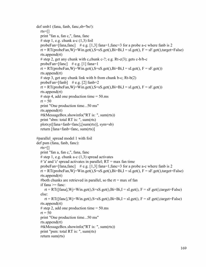
169

def smb1 (fana, fanb, fanc,sb='bo'):

rts=[]

print "fan a, fan c,", fana, fanc

# step 1, e.g. chunk a-c (1,3) foil

probeFan=[fana,fanc] # e.g. [1,3] fana=1,fanc=3 for a probe a-c where fanb is 2

rt = RT(probeFan,Wj=Win.get(),S=sS.get(),Bi=Bi,I = sI.get(), F = sF.get(),target=False)

rts.append(rt)

# step 2, get any chunk with c,chunk c-?; e.g. Rt-c(3); gets c-b/b-c

probeFan=[fanc] # e.g. [1] fana=1

rt = RT(probeFan,Wj=Win.get(),S=sS.get(),Bi=Bi,I = sI.get(), F = sF.get())

rts.append(rt)

# step 3, get any chunk link with b from chunk b-c; Rt-b(2)

probeFan=[fanb] # e.g. [2] fanb=2

rt = RT(probeFan,Wj=Win.get(),S=sS.get(),Bi=Bi,I = sI.get(), F = sF.get())

rts.append(rt)

# step 4, add one production time = 50.ms

rt = 50

print "One production time...50 ms"

rts.append(rt)

#tkMessageBox.showinfo("RT is: ", sum(rts))

print "sbm: total RT is: ", sum(rts)

plotxy([fana+fanb+fanc],[sum(rts)], sym=sb)

return [fana+fanb+fanc, sum(rts)]

#parallel_spread model 1 with foil

def psm (fana, fanb, fanc):

rts=[]

print "fan a, fan c,", fana, fanc

# step 1, e.g. chunk a-c (1,3) spread activates

# 'a' and 'c' spread activates in parallel; RT = max fan time

probeFan=[fana,fanc] # e.g. [1,3] fana=1,fanc=3 for a probe a-c where fanb is 2

rt = RT(probeFan,Wj=Win.get(),S=sS.get(),Bi=Bi,I = sI.get(), F = sF.get(),target=False)

rts.append(rt)

#both chunks are retrieved in parallel, so the rt = max of fan

if fana >= fanc:

rt = RT([fana],Wj=Win.get(),S=sS.get(),Bi=Bi,I = sI.get(), F = sF.get(),target=False)

else:

rt = RT([fanc],Wj=Win.get(),S=sS.get(),Bi=Bi,I = sI.get(), F = sF.get(),target=False)

rts.append(rt)

# step 2, add one production time = 50.ms

rt = 50

print "One production time...50 ms"

rts.append(rt)

#tkMessageBox.showinfo("RT is: ", sum(rts))

print "psm: total RT is: ", sum(rts)

return sum(rts)

170

def psm1 (fana, fanb, fanc, sb='go'):

rts=[]

print "fan a, fan c,", fana, fanc

# step 1, e.g. chunk a-c (1,3) spread activates

# 'a' and 'c' spread activates in parallel; RT = max fan time

probeFan=[fana,fanc] # e.g. [1,3] fana=1,fanc=3 for a probe a-c where fanb is 2

rt = RT(probeFan,Wj=Win.get(),S=sS.get(),Bi=Bi,I = sI.get(), F = sF.get(),target=False)

rts.append(rt)

#both chunks are retrieved in parallel, so the rt = max of fan

if fana >= fanc:

rt = RT([fana],Wj=Win.get(),S=sS.get(),Bi=Bi,I = sI.get(), F = sF.get(),target=True)

else:

rt = RT([fanc],Wj=Win.get(),S=sS.get(),Bi=Bi,I = sI.get(), F = sF.get(),target=True)

rts.append(rt)

# step 2, add one production time = 50.ms

rt = 50

print "One production time...50 ms"

rts.append(rt)

#tkMessageBox.showinfo("RT is: ", sum(rts))

print "psm: total RT is: ", sum(rts)

plotxy([fana+fanb+fanc],[sum(rts)], sym=sb)

return [fana+fanb+fanc, sum(rts)]

#parallel_spread model 2: without foil

def psm2 (fana, fanb, fanc):

rts=[]

print "fan a, fan c,", fana, fanc

# step 1, e.g. chunk a-c (1,3) spread activates

# 'a' and 'c' spread activates in parallel; RT = max fan time

probeFan=[fana,fanc] # e.g. [1,3] fana=1,fanc=3 for a probe a-c where fanb is 2

## rt = RT(probeFan,Wj=Win.get(),S=sS.get(),Bi=Bi,I = sI.get(), F =

sF.get(),target=False)

## rts.append(rt)

#both chunks are retrieved in parallel, so the rt = max of fan

if fana >= fanc:

rt = RT([fana],Wj=Win.get(),S=sS.get(),Bi=Bi,I = sI.get(), F = sF.get(),target=True)

else:

rt = RT([fanc],Wj=Win.get(),S=sS.get(),Bi=Bi,I = sI.get(), F = sF.get(),target=True)

rts.append(rt)

# step 2, add one production time = 50.ms

rt = 50

print "One production time...50 ms"

rts.append(rt)

#tkMessageBox.showinfo("RT is: ", sum(rts))

print "psm: total RT is: ", sum(rts)

return sum(rts)

171

def psm21 (fana, fanb, fanc, sb='rs'):

rts=[]

print "fan a, fan c,", fana, fanc

# step 1, e.g. chunk a-c (1,3) spread activates

# 'a' and 'c' spread activates in parallel; RT = max fan time

probeFan=[fana,fanc] # e.g. [1,3] fana=1,fanc=3 for a probe a-c where fanb is 2

## rt = RT(probeFan,Wj=Win.get(),S=sS.get(),Bi=Bi,I = sI.get(), F =

sF.get(),target=False)

## rts.append(rt)

#both chunks are retrieved in parallel, so the rt = max of fan

if fana >= fanc:

rt = RT([fana],Wj=Win.get(),S=sS.get(),Bi=Bi,I = sI.get(), F = sF.get(),target=False)

else:

rt = RT([fanc],Wj=Win.get(),S=sS.get(),Bi=Bi,I = sI.get(), F = sF.get(),target=False)

rts.append(rt)

# step 2, add one production time = 50.ms

rt = 50

print "One production time...50 ms"

rts.append(rt)

#tkMessageBox.showinfo("RT is: ", sum(rts))

print "psm: total RT is: ", sum(rts)

plotxy([fana+fanb+fanc],[sum(rts)], sym=sb)

return [fana+fanb+fanc, sum(rts)]

#classic fan model: simple fan-effect model

def sfm (fana, fanb, fanc):

rts=[]

print "fan a, fan c,", fana, fanc

# step 1, e.g. chunk a-c (1,3) spread activates

# 'a' and 'c' spread activates in parallel; RT = normal fan effect RT

rt = RT([fana, fanc],Wj=Win.get(),S=sS.get(),Bi=Bi,I = sI.get(), F =

sF.get(),target=False)

rts.append(rt)

# step 2, add one production time = 50.ms

rt = 50

print "One production time...50 ms"

rts.append(rt)

#tkMessageBox.showinfo("RT is: ", sum(rts))

print "simple fan sfm: total RT is: ", sum(rts)

return sum(rts)

def sfm1 (fana, fanb, fanc, sb='bs'):

rts=[]

print "fan a, fan c,", fana, fanc

# step 1, e.g. chunk a-c (1,3) spread activates

# 'a' and 'c' spread activates in parallel; RT = normal fan effect RT

172

rt = RT([fana, fanc],Wj=Win.get(),S=sS.get(),Bi=Bi,I = sI.get(), F =

sF.get(),target=False)

rts.append(rt)

# step 2, add one production time = 50.ms

rt = 50

print "One production time...50 ms"

rts.append(rt)

#tkMessageBox.showinfo("RT is: ", sum(rts))

print "simple fan sfm: total RT is: ", sum(rts)

plotxy([fana+fanb+fanc],[sum(rts)], sym=sb)

return [fana+fanb+fanc, sum(rts)]

#****************

# a function for models to process a list of lists of fans; it works with plot option

# input: a list of lists of fanouts for a set of probes e.g. [[1,1],[1,2],...]

# returns/output: target rt

# uses: it calls RT for each item in the input list

# model usage: e.g. doList([ [1,2], [1,3], [1,4]])

def doList (inlist, Wi=Wj, Si=S, Bin=Bi,Ii = I, Fi = F):

fan=[] # a list of total fan for target plot

csv=[] # a list of rts for target plot

#loop through each item ( fan_jsi) from the input list

for item in inlist: # input list e.g. [[1,1],[1,2],...]

rt = RT(item, Wj=Wi, S=Si, Bi=Bin, I =Ii,F =Fi )

total_fan = sum(item)

fan.append(total_fan)

csv.append(rt)

print "x-list - total fan : ", fan

print "y_list - fan_rt : ", csv

# run options: 'save' and 'plot' for the results

#----------------------------------------------

# plot

if vplot.get():

plotxy(fan,csv,'bs')

#save fan_rts results to fanresult.csv; merging two lists into one

if logstatus.get():

#making a list of lists with two variables total_fan and RT

i = 0

fanrt = []

for x in fan:

fanrt.append([str(x),str(csv[i])])

i +=1

print "for csv ", fanrt

results = open('fanresult.csv', 'w')

173

for x in fanrt: results.write(','.join(x) +'\n')

results.close()

#****** run GUI and main

root.config(menu=menubar)

root.mainloop()

174

Appendix B Tool#2: Dataset Fan Checker

To calculate a reaction time for fan or complex fan analysis requires the calculation

of the fans in a probe; the fans in a probe are a function of the data set. The fans are then

entered into each of the different models to calculate an RT data point for the models. This

calculation must be repeated for each probe and for all the probes. The calculating process is

laborious and the management of this process for multiple models is error prone. A second

tool: the data set fan-checker has been developed to mitigate this situation.

The data set fan-checker is a tool developed to support the complex fan analysis and

the data recording for the experiments. The fan checker ensures the right fan number is used

for a RT calculation for each probe in all the models and in different experiments where the

data set is changing. The data set fan checker parses through the test data set of the

experiment and provides the right fan numbers for each probe and hence the appropriate RT

predictions for the probe.

Figure B-1 shows how a fan of an object is calculated. For example, to calculate the

fan for “box” (a concept) in a data set, the data set fan-checker is loaded with the test data

set for the experiment using the “File to Fan-dictionary” function. The term “box” is entered

into the “Fan check text field”. Apply the “Fan check” function, the result shows that the

element “box” has a fan of 1 with respect to the entire test data set.

175

Figure B-1 A Sample Output of the Fan-Checker

Figure B-2 A Sample Output of a Changed Fan

176

In a multi-step model, the test dataset can change over the course of the experiment,

and new calculations may be required to determine the number of fans. To support such

variability, the fan-checker function is used dynamically. For example, repeating the same

procedure; loading a new test data set for a different experiment and check for the fan

“box”. Figure B-2 shows that the fan result for “box” is now 2. The core fan checking

functions have been incorporated as a part of the experiment apparatus for the complex fan

experiments.

177

B.1 Dataset Fan Checker code

# Complex Fan - Fan Checker

# Purpose: to claculate the fans for each chunk based on a test data set

#

# Author: Kam Kwok , 2013, 2014

from Tkinter import *

import random

import math

import tkFileDialog

###

# global variables for input (inlist) and output (anslist)

anslist=[]

ca = 0

# d - word count dictionary

wd = {}

# fd - fan dictionary build up by fdict()

fd={}

# fl - fan list, the displyed output

fl=[]

t = '' # search target string

infilelist=[]

###

# Place-holder functions

def future():

print "Coming soon."

def donothing():

filewin = Toplevel(tk)

button = Button(filewin, text="Do nothing button")

button.pack()

def about():

filewin = Toplevel(tk)

l0 = Label(filewin, text="Kam Kwok, copyright 2014\nEmail: kwok.kam@gmail.com")

l0.pack()

def msg(m):

if type(m)<> str: m =str(m)

filewin = Toplevel(tk)

l0 = Label(filewin, text="msg: "+m)

l0.pack()

178

def onclick():

pass

###

# utility functions

#File to list; Called by Qtest for targets

def openf2l(fs):

f = open(fs,'r')

l = f.readlines()

f.close

return ([str.strip(line) for line in l])

# used by count_t; count_all in a file; mode: 'w'=word, 'a'=alphbet'

def count(inputline,wd,mode='w'):

if mode == 'w':

sequence = inputline.split()

elif mode == 'a':

sequence = inputline

for x in sequence:

if wd.has_key(x):

wd[x] += 1

else:

wd[x] = 1

# add word count(from input line) to word dictionary wd, using count(); t for target search

def count_t(inputline,wd,target=''):

if target == '':

# count_all call count

count (inputline,wd,'w')

else:

sequence = inputline.split()

for x in sequence:

if x == target:

if wd.has_key(x):

wd[x] += 1

else:

wd[x] = 1

# Update fan dictionary (fd) with the inputline and word dictionary (wd)

def fdict(inline):

global fd,wd,fl

ft=[]

inline=inline.strip()

sequence = inline.split()

for x in sequence:

if wd.has_key(x):

179

ft.append (wd[x])

else:

ft.append (0)

fl.append((inline,ft))

fd[inline]=ft

# use by addrec to append a csv record to usr

def app2csv(usr, rStr):

session = open(usr+'.csv', 'a')

session.write(rStr)

session.close()

# This takes list as input record; each element in the list becomes a csv field

def addrec(fs='test',lst=[]):

## savrec = ','.join(lst)+'\n'

savrec = ','.join(lst)+'\n'

app2csv(fs, savrec)

# read a file to create a word dictionary (wd) and fan dictionary (fd)

def b_f2fandict():

global wd, fl, fd, infilelist

try:

f= tkFileDialog.askopenfile(parent=tk,mode='rb',title='Choose a file')

#reset global variables

wd={}

fd={}

fl=[]

infilelist=[]

f.seek(0,0)

#create wd

count_t(f.read(),wd,t)

#create fd with fdict()

f.seek(0,0)

for line in f.readlines():

infilelist.append(line)

fdict(line)

f.close()

ftext.insert(INSERT, fl)

for elem in fl:

addrec(fs='f2dprobes', lst=[elem[0],str(elem[1])])

ftext.insert(INSERT, 'Appended to f2dprobes.csv !\n')

except:

ftext.insert(INSERT, 'Error or no file selected.')

# b clear

def b_clr():

ftext.delete(1.0, END)

eText.set('')

180

# gen a list based on input 'range' and 'operator'; returns a list

def mgen(r,o):

rs=[]

for i in range(r):

for j in range(r):

ans= eval(str(i)+o+str(j))

rse = str(i)+' '+str(o)+' '+str(j)+' '+'='+' '+ str(ans)

rs.append(rse)

return rs

def b_mgen():

global infilelist,wd,fl

infilelist.extend(mgen(10,'+'))

infilelist.extend(mgen(10,'*'))

#create a dict-d

for l in infilelist:

count_t(l,d)

#create fan dictionary

for l in infilelist:

fdict(l)

ftext.insert(INSERT, 'OK!\n')

# Output fan list as a fan dictionary; print fd

def b_pfd():

try:

#ftext.insert(INSERT, fl)

plist=[fle[0]+','+str(fle[1])+'\n' for fle in fl]

for li in plist:

addrec(fs='Fandictionary',lst=li)

ftext.insert(INSERT, 'Fandictionary created!\n')

except:

ftext.insert(INSERT, 'Error:cannot save!\n')

# Input a probes file output a fan list as a fan dictionary,; it uses wd, and fd

def b_prbfile2d():

global wd, fl, fd, infilelist

try:

f= tkFileDialog.askopenfile(parent=tk,mode='rb',title='Choose a file')

for line in f.readlines():

# a list of three elements: line, fanlist, tptal fan

rfc=fancheck(line)

addrec(fs='probefans', lst=[rfc[0],str(rfc[1]), str(rfc[2])])

except:

ftext.insert(INSERT, 'Error:cannot save!\n')

ftext.insert(INSERT, 'probefans.csv is saved!\n')

181

def cfRT(inline,target=True):

global fd,wd,cftflst

#input: a list of concepts; returns: a list of fans and RT

def calrt(conceptlist, target1=True):

ft=[] # the fans list

rs='' # ft in string

# Associative strength

S=1.45

# base level activation: recency and frequency

Bi=0

#Intercept

I = 845

#F scaling factor

F= 613

sum_wj_sji =0

#Wj list

wlist=[]

# use concept list to create w-list

for x in conceptlist:

if len(conceptlist) > 3:

wlist.append(1.0/len(conceptlist))

else:

wlist.append(0.333)

if wd.has_key(x):

ft.append (wd[x])

rs=rs+str (wd[x])+','

else:

ft.append (1)

rs=rs+str ('1,')

# calculate target or foil

if target1:

for f,w in map(None,ft,wlist):

ln_fan_j = math.log(f)

Sji = S-ln_fan_j

sum_wj_sji = sum_wj_sji + (w*Sji)

Ai = Bi+sum_wj_sji

rt = I+F*math.exp(-Ai)

else: # foil calculation

rt_foils = []

for f,w in map(None,ft,wlist):

ln_fan_j = math.log(f)

Sji = S-ln_fan_j

sum_wj_sji = w*Sji # set sum to individual Sji

Ai = Bi+sum_wj_sji

rtf = I+F*math.exp(-Ai)

182

rt_foils.append(rtf) # a list of rt(fan)

foil_rt = sum(rt_foils)/len(rt_foils) # foil = average singles

rt = foil_rt

return (ft,float("%4.2f" % rt))

inline=inline.strip()

obj= inline.split()[0]

location= inline.split()[-1]

container='unknown'

sequence = inline.split()

if 'in' in sequence: sequence.remove('in')

# get obj-loc string

sstr= ' '.join(sequence)

# cftflist rec format: 'obj location container'; get container

for r in cftflst:

if sstr in r:

container= r.split()[-1]

found = True

# Serial forward model and serial backward model with foil

sfmrt=0.0

sbmrt=0.0

pmrt=0.0

pmnfrt=0.0

# step 1 cal rt for foil on obj-loc for sfm and sbm

ollist= [obj,location]

olfoil= calrt(ollist,target1=False)[1]

sfmrt=olfoil

sbmrt=olfoil

pmrt=olfoil

# step 2 cal rt for obj-fan;for sfm

objlist=[obj]

objrt= calrt(objlist,target1=True)[1]

sfmrt= sfmrt+objrt

# step 3 cal rt for container-fan sfm and step 3 for sbm

contlist=[container]

contrt=calrt(contlist,target1=True)[1]

sfmrt= sfmrt+contrt

sbmrt= sbmrt+contrt

# step 2 cal rt for container-fan sbm

loclist=[location]

locrt=calrt(loclist,target1=True)[1]

sbmrt= sbmrt+locrt

# longest rt between obj and loc; pmnfrt - parallel no foil rt

if objrt > locrt:

pmrt=pmrt+objrt

pmnfrt=objrt+50.0

else:

183

pmrt=pmrt+locrt

pmnfrt=locrt+50.0

# step 4 add one production cycle = 50 ms for sfm and sbm rts

sfmrt= sfmrt+50.0

sbmrt= sbmrt+50.0

pmrt=pmrt+50.0

#two steps rts

oclist=[obj,container]

objconrt=calrt(oclist,target1=target)

cllist=[container, location]

conlocrt=calrt(cllist,target1=target)

ollist=[obj,location]

objlocrt=calrt(ollist,target1=target)

#return (oclist,objconrt,cllist,conlocrt,sfmrt)

return (str(objconrt[0]).strip('[]'), str(objconrt[1]),str(conlocrt[0]).strip('[]'),

str(conlocrt[1]),container,

str(objlocrt[0]).strip('[]'), str(objlocrt[1]), str(sfmrt),

str(sbmrt),str(pmrt),str(pmnfrt),str(olfoil))

def RT(inline,target=TRUE):

global fd,wd

ft=[] # the fans list

rs='' # ft in string

S=1.45

Bi=0

I = 845

F= 613

sum_wj_sji =0

wlist=[]

inline=inline.strip()

sequence = inline.split()

if 'in' in sequence: sequence.remove('in')

for x in sequence:

if len(sequence) > 3:

wlist.append(1.0/len(sequence))

else:

wlist.append(0.333)

if wd.has_key(x):

ft.append (wd[x])

rs=rs+str (wd[x])+','

else:

ft.append (1)

rs=rs+str ('1,')

if target: # calculate target

#for x, y in map(None, a, b):

for f,w in map(None,ft,wlist):

184

ln_fan_j = math.log(f)

Sji = S-ln_fan_j

sum_wj_sji = sum_wj_sji + (w*Sji)

Ai = Bi+sum_wj_sji

rt = I+F*math.exp(-Ai)

else: # foil calculation

rt_foils = []

for f,w in map(None,ft,wlist):

ln_fan_j = math.log(f)

Sji = S-ln_fan_j

sum_wj_sji = w*Sji # set sum to individual Sji

Ai = Bi+sum_wj_sji

rtf = I+F*math.exp(-Ai)

rt_foils.append(rtf) # a list of rt(fan)

foil_rt = sum(rt_foils)/len(rt_foils) # foil = average singles

rt = foil_rt

return float("%4.2f" % rt)

#fanlist, wlist to RT

def ftrt(flist, wjlist, probeT):

if probeT: # calculate target

#for x, y in map(None, a, b):

for f,w in map(None,flist,wjlist):

ln_fan_j = math.log(f)

Sji = S-ln_fan_j

sum_wj_sji = sum_wj_sji + (w*Sji)

Ai = Bi+sum_wj_sji

rt = I+F*math.exp(-Ai)

else: # foil calculation

rt_foils = []

for f,w in map(None,flist,wjlist):

ln_fan_j = math.log(f)

Sji = S-ln_fan_j

sum_wj_sji = w*Sji # set sum to individual Sji

Ai = Bi+sum_wj_sji

rtf = I+F*math.exp(-Ai)

rt_foils.append(rtf) # a list of rt(fan)

foil_rt = sum(rt_foils)/len(rt_foils) # foil = average singles

rt = foil_rt

return float("%4.2f" % rt)

#inputline to RT

def lineRT(inline,target=TRUE):

global fd,wd

ft=[] # the fans list

rs='' # ft in string

185

S=1.45

Bi=0

I = 845

F= 613

sum_wj_sji =0

wlist=[]

inline=inline.strip()

sequence = inline.split()

if 'in' in sequence: sequence.remove('in')

for x in sequence:

if len(sequence) > 3:

wlist.append(1.0/len(sequence))

else:

wlist.append(0.333)

if wd.has_key(x):

ft.append (wd[x])

rs=rs+str (wd[x])+','

else:

ft.append (1)

rs=rs+str ('1,')

return ftrt(flist=ft,wjlist=wlist,probeT=target)

###

# GUI widgets

# add menu and commands

#instantiate a Tk object - tk

tk = Tk(className=" Data Set Fan Checker")

# option

##tk = Tk()

##tk.title("Complex Fan Effect Lab")

# full screen start-up

##w, h = tk.winfo_screenwidth(), tk.winfo_screenheight()

##tk.geometry("%dx%d+0+0" % (w, h))

# create menubar obj with a Tk object - tk

menubar = Menu(tk)

filemenu = Menu(menubar, tearoff=0)

filemenu.add_command(label="New", command=donothing)

filemenu.add_command(label="Open", command=donothing)

filemenu.add_command(label="Save", command=donothing)

filemenu.add_command(label="Save as...", command=donothing)

filemenu.add_command(label="Close", command=donothing)

filemenu.add_separator()

186

filemenu.add_command(label="Exit", command=tk.destroy)

menubar.add_cascade(label="File", menu=filemenu)

editmenu = Menu(menubar, tearoff=0)

editmenu.add_command(label="Undo", command=donothing)

editmenu.add_separator()

editmenu.add_command(label="Cut", command=donothing)

editmenu.add_command(label="Copy", command=donothing)

editmenu.add_command(label="Paste", command=donothing)

editmenu.add_command(label="Delete", command=donothing)

editmenu.add_command(label="Select All", command=donothing)

menubar.add_cascade(label="Edit", menu=editmenu)

helpmenu = Menu(menubar, tearoff=0)

helpmenu.add_command(label="Help Index", command=donothing)

helpmenu.add_command(label="About...", command=about)

menubar.add_cascade(label="Help", menu=helpmenu)

tk.config(menu=menubar)

# give a vertical scrollbar to tk

scrollbar = Scrollbar(tk)

scrollbar.pack(side='right', fill='y')

# create a frame in tk

frame = Frame(tk)

frame.pack()

# Output widgets

# create a label - an output or display widget; var = output-label-str-var (olsv)

##olsv=StringVar()

##Label(frame, textvariable = olsv,text="Helvetica", font=("Helvetica", 28)).pack()

### set label

##olsv.set("Word Frequency and Fan Check")

# creating text boxes

# Input output or editing widget

# for loading in file data

##ftext = Text(frame, width=200, height = 5)

##ftext.pack()

ftext = Text(frame)

ftext.pack(fill=BOTH)

# user input box

##itext = Text(frame, width=20, height = 1)

187

##itext.pack()

### fixed label

##L1 = Label(frame, text="Model file spec.")

##L1.pack()

##L1sv=StringVar()

##Label(frame, textvariable = L1sv,text="Helvetica").pack()

### set label

##L1sv.set("Search file")

### file spec box

##E1 = Entry(frame, text="NT.txt", bd =5)

##E1.pack()

### target lable and entry

##L2=Label(frame, text="Target")

##L2.pack()

### target box

##E2 = Entry(frame, bd =5)

##E2.pack()

##

### button for file

##b_f = Button(frame,text="1. Select file",width=20, command=b_openf)

##b_f.pack()

# clause box

# Button widget

b_fd = Button(frame,text="File to Fan-dictionary ",width=20, command=b_f2fandict)

b_fd.pack()

L3=Label(frame, text="Fan check: enter a clause")

L3.pack()

eText = StringVar()

e3 = Entry(frame, bd=5,textvariable=eText)

e3.pack()

# Fan check: input a string, it uses wd and fd fan dictionary to report fans associations

def b_fc():

global fd,wd # the word and fan dictionaries

line = eText.get()

fc = 0

fanl=[]

for word in line.split():

try:

if wd[word]:

fc = fc + wd[word]

fanl.append(wd[word])

except:

wd[word]=1

fc = fc+ 1

188

fanl.append(1)

ftext.insert(INSERT, fc)

ftext.insert(INSERT, '\n')

rrt = 'reaction times: ' + str(RT(line))

ftext.insert(INSERT, rrt)

ftext.insert(INSERT, '\n')

try:

res=line + ': '+ str(fanl)

ftext.insert(INSERT, res)

ftext.insert(INSERT, '\n')

except:

ftext.insert(INSERT, "not in dictionary")

ftext.insert(INSERT, '\n')

#msg(fc)

return fc

# Fan check: input a string, it uses wd and fd fan dictionary to report fans associations

def b_cffc():

global fd,wd # the word and fan dictionaries

line = eText.get()

cfrtresult=cfRT(line)

rrt = 'reaction times: ' + str(cfrtresult)

ftext.insert(INSERT, rrt)

ftext.insert(INSERT, '\n')

# Fan-check: input a string, it uses wd and fd fan dictionary to report fans associations

# Used by probe file to dictionary

def fancheck(instr):

global fd,wd # the fan dictionary

line = instr

fc = 0

fanl=[]

for word in line.split():

try:

if wd[word]:

fc = fc + wd[word]

fanl.append(wd[word])

except:

wd[word]=1

fc = fc+ 1

fanl.append(1)

return [line, fanl,fc]

#eText.set/get("...I'm not inserted, I've just appeared out of nothing.")

b_pars = Button(frame,text="Fan check",width=20, command=b_fc)

b_pars.pack()

189

b_pars = Button(frame,text="Complex Fan check",width=20, command=b_cffc)

b_pars.pack()

b_mathgen = Button(frame,text="math facts gen.",width=20, command=b_mgen)

b_mathgen.pack()

# button for user input

b_clr = Button(frame,text=" Clear all",width=20, command=b_clr)

b_clr.pack()

b_prtfd = Button(frame,text="Create probe-fan file",width=20, command=b_prbfile2d)

b_prtfd.pack()

##

### Input widgets

### create a scale/slider;

### use gs.get() in handlers to obtain slider value (score)

##score=IntVar(value = 0)

##gs = Scale(frame, label = "Not gray<"+ "-"*95 +">more gray", variable=score,

length=1000, font=("Helvetica", 18),

## from_=0, to=9, tickinterval=1, resolution=1, orient='horizontal')

##gs.pack()

##

##b_prg = Button(frame,text=" print globals ",width=20, command=b_prg)

##b_prg.pack()

### Tk object eventloop

# setup CF targets fans list for cfRT calculation

cftflst=openf2l('cfcontainers.txt')

tk.mainloop()

root.mainloop()

190

Appendix C Tool#3: The Virtual Mind Framework for Python ACT-R

A pilot study has been conducted to explore the retrieval based inference

questions: could relational inferences simply be a union of two facts? A Python ACT-R

model has been constructed to examine the sufficiency of a set of associative production

rules and to examine how a set of associative rules or productions can achieve relational

inferences at the behavior level. A simple set of production rules for unions of

propositions has been defined for a “virtual mind” agent.

Python ACT-R (T. Stewart & West, 2006) is an re-implementation of the ACT-R

theory in Python language syntax. Python ACT-R facilitates exploration and integration

of the core ACT-R theory with other cognitive models or new modules based on a

simpler interface of the Python programming language. It enables the application of the

ACT-R theory without the constraints of the lisp language syntax and facilitates the use

of basic ACT-R components such as the declarative memory system in new ways.

The virtual mind framework has been developed as part of this dissertation for

modeling complex fan tasks. Moreover, the virtual mind framework is designed to

support the development of any complex model that has compound interdependent

productions - protoyping for production sets. The Virtual mind framework facilitates the

design, testing and validation of the interdependent production rules for a model by

enabling an interactive and incremental development process for production rules. This

framework turns a complex development task into a series of simpler building block

designs.

The key feature of the virtual mind framework is an interactive interface between

the experimenter and the cognitive model in Python ACT-R. The interface acts as a part

of the executive control module. In general, a virtual mind agent consists of a declarative

memory, a production module, a motor module and a “focus buffer” which serves as the

executive control function. A virtual mind framework based agent can interact with a

191

simple environment with objects in the environment and the agent can also interact with

the experimenter through the focus buffer via a set of commands which functions as a

part of the executive control. This command interface feature is important for two

reasons: first, it provides an interactive mode for cognitive model development which is

important for the understanding of the behavior of the model as well as for the debugging

of the model. Second, the interactive mode provides incremental or step-wise flexibility

for the execution of multiple strategies or tasks (by selecting different set of productions)

and a modular approach for testing related productions. In the virtual mind framework,

the agent‟s goals are defined and introduced into the focus buffer by the experimenter.

The behavior of the agent is influenced by these commands. The input of commands and

output of the agent are displayed through the program console.

As a pilot study, a relational inference model has been implemented with the

virtual mind framework. At the initialization of the model, a complex fan environment

(CFE) is created. An agent is instantiated in CFE. The agent‟s executive control monitors

the command input from the experimenter. The agent is designed with productions to

respond to the commands. Unlike the conventional artificial intelligence programming,

the production rules for an ACT-R agent are rules for memory retrieval and goal buffer

matching rules. There are no high-level programming construct such as “if „this‟ do

„that‟” in the model. All high-level cognitive tasks are built from basic memory-buffer

operations. For example, the inference task described in Table D-1 is a series of memory

retrieval and goal buffer matching steps. In terms of complex fan, the production rules are

simply target and foil recognition rules. ACT-R productions are constrained by the ACT-

R architecture. The productions for the inference model are also restricted to process

memory chunks with specific structure for a specific type of experiment. For example, in

the fan experiment, propositions are assumed to have three slots: a subject slot, a relation

slot and an object slot. The structure for the chunk “box in pool” is represented as

192

“subject:box relation:in object:pool”. The details for these productions are described in

the model code documented in Appendix C.2.

The following is a list of commands that the inference model agent currently

supports:

„s‟ for recalling a proposition from declarative memory based on the subject slot.

The experimenter can request the agent to recall a proposition base on an input subject.

'o' for recalling a proposition from declarative memory based on the object slot.

The experimenter can request the agent to recall a proposition base on an input object.

'r' for recalling a proposition from declarative memory based on the relation slot.

The experimenter can request the agent to recall a proposition base on an input relation.

'e' for entering or learning a new proposition for the agent. The experimenter can

enter a new proposition for the agent to learn.

'env' for the agent to scan the environment for any object. The experimenter can

request the agent to scan the environment.

'p' for putting an object in the environment. The experimenter can request the

agent to put an object in the environment as a new subject or object for proposition

processing.

„q‟ for the agent to assess if an input proposition is true. This command is used by

the experimenter to evaluate the agent‟s ability to infer based on the input and its

knowledge in declarative memory.

„g‟ for the generation of new propositions from the knowledge in memory. The

experimenter can request the agent to deduce new knowledge based on the agent‟s

knowledge. This command is used by the experimenter to evaluate the agent‟s ability to

deduce new information autonomously thereby creating new knowledge based on the

inference process.

„f‟ for the generation of new knowledge from existing knowledge in memory

based on cues in the environment. This command instructs the agent to scan for a cue

from the environment and deduce new information.

„l‟ for initializing loading up declarative memory with a set of propositions from

a text file. This is a utility command for providing the agent with knowledge from a pre-

defined text file.

„x‟ will stop and exit the model.

These commands are designed to enable the experimenter to perform small-step

experiments by interacting with the agent.

193

C.1 Python ACT-R Inference Virtual Mind Simulation

Figure C-1 shows the user interface for a relational inference agent (based on the

high-level task analysis described in Table D-1). Figure C-2 shows a session sample of

the simulation. Two propositions are entered into the agent‟s memory “box in pool” and

“ring in box”. The agent is then directed to infer from the object “ring”. The agent uses

multiple memory retrieval productions to reach a correct deduction that “ring in pool”; a

new fact has been derived from its knowledge. The derivation of the production rules for

the model is a straight forward task given a high-level task analysis. Each step is

translated into a set of productions which includes error handling for conditions such as

memory is busy or empty retrieval etc.

Figure C-1 A Virtual Mind Inference Agent Interface

194

Figure C-2 a Virtual Mind Simulation for Inference

195

C.2 Virtual Mind Framework module code

#################### Virtual mind framework ###################

# Model: Virtual mind framework version 24

# Date: 2012-04-18

# Author: Kam Kwok

# Purpose: to create a framework and model for storing chunks,retrieving chunks and

deducing new chunks from declarative memory.

# Notes:

# The model consists of an environment (cfe), an agent(kam), the agent has a motor

module.

# the user is a part of the environment, which provides commands/suggestions to the

mind.

# A chunk is a collection of concepts/cues.

# DM request and DM add using slot name

#################### ------------###################

#***********************

# 1. set up ACT-R library/framework for constructing the model; setup runtime log

#***********************

#the following three line are used for running the model from desktop

##import sys

##sys.path.append('C:\Users\Kam\Desktop\CCMSuite')

##sys.path.append('C:\Users\Kam\Documents\CCMSuite')

import ccm

log=ccm.log()

from ccm.lib.actr import *

#####

# Python ACT-R requires an environment

# (if we are not using anything in the environment

# we can use 'pass' instead)

#***********************

# 2.Define an environment

#***********************

class MyEnvironment(ccm.Model):

# 'def start(self):' is an initialization production

# The environment and the agent is the model.

# Define all global functions and var in the environment. to call it use: self.parent. etc.

# a). get_input is called by the agent at initialization

# Initialize items in the environment; items in the environment look and act like chunks

(in buffers) - but note the syntactic difference ('=' vs ':')

# these are objects in the env with attributes initialized to blank strings

196

env_obj=ccm.Model(word='')

subject_icue=ccm.Model(subject='')

relation_icue=ccm.Model(relation='')

object_icue=ccm.Model(object='')

rehearsalDB = {} # definition: {(chunk:count)...} chunk rehersal

count database - base activation counts

#Rehearsal counts for base activation - set up tools in the env

def RhsCount(self,fact):

if self.rehearsalDB.has_key(fact):

self.rehearsalDB[fact] +=1

else:

self.rehearsalDB[fact] = 1

#print "Base activation DB: ", self.rehearsalDB

# Main loop - the mind loop, the brain/agent is receiving a command/suggestion;

# When the agent's attention/focus/goal buffer = 'init_loop' will direct the agent to look

for a command here;

# The agent will execute parent.get_input() at the end of each cognitive task.

# This is an interaction menu implementation - task switching here.

# the environment gets input from the user(agent) and sets the mind's/agent's focus.

# the agent init() calls the get_input function

def get_input(self):

while 1: # loop forever to get user suggestion - any invalid command is ignored

print ""

choice = raw_input("Please enter a command letter and hit 'return': ")

if choice == 's':

kam.focus.set('s_recall') # recall with a subject (s)

break # exit loop

elif choice == 'o':

kam.focus.set('o_recall') # recall with an object (o)

break # exit loop

elif choice == 'e':

fact = raw_input("Please enter a three word fact <subject> <relationship>

<object>: ")

wl= fact.split()

print "I have: ", wl

#print wl[0],wl[1],wl[2]

#Trick1 or Trick2 use pre-processed string as an input to .add; DM chunk

structure: subject:<s> relation:<r> object:<o>

# e for enter a chunk into DM

kam.DM.add('subject:'+wl[0]+' relation:'+wl[1]+' object:'+wl[2])

elif choice == 'q': # q for query/process if a statement is true...

kam.imaginal.clear()

qfact = raw_input("Please enter a three word fact: ")

197

kam.imaginal.set(qfact) #imaginal stores user's input fact; go to deduce/process

kam.focus.set('deduce')

break # exit loop

elif choice == 'g':

kam.focus.set('get_f1')

break # exit loop

elif choice == 'r':

kam.focus.set('r_recall')

break # exit loop

elif choice == 'f':

kam.motor.focusSubject() # focus on the object in env

break # exit loop

elif choice == 'p':

kam.motor.SetEnvSubject() # put object in env

break # exit loop

elif choice == 'd':

kam.focus.set('d_facts') # display initial facts

break # exit loop

elif choice == 't':

kam.focus.set('set_img') # set and switch Imaginal

break # exit loop

elif choice == 'l':

kam.motor.LoadFile('') # load a data file <fn>.txt : subject:<value>

relation:<value> object:<value>

break # exit loop

elif choice == '?':

kam.motor.Disp_cmd()# display commands

elif choice == 'env':

#kam.motor.Disp_env()

kam.focus.set('recall_env')

break # exit loop

elif choice == 'x':

kam.focus.set('stop')

break # exit loop

else:

kam.motor.Disp_cmd()# display commands

#break # exit loop

# b). or alternatively store initial chunks here ...

#***********************

# 2.1 Define other modules such as a motor module or a vision module in the env; these

modules are used by the agent to look and act on the objects in the env (cfe - buffers)

#***********************

class MotorModule(ccm.Model): # create a motor/vision module to carry out actions;

motor is a child of the agent/mind

def focusSubject(self): # note that technically the motor module is outside the agent

198

# this production checks on two buffers: focus and subject_icue

self.parent.focus.set('s_recall_env') # the parent is the agent:kam

def Disp_env(self):

self.parent.focus.set('recall_env')

# cmd:?

def Disp_cmd(self):

print

print "The mind is thnking about what it should do."

print "you can enter a command to help it to decide."

print

print "*** Command Menu ****"

print

print "'s' for recall by subject"

print "'o' for recall by object"

print "'e' for entering a new fact into memory"

print "'env' for examining the environment"

print "'q' for true or false query"

print "'g' for generating a new fact using deduction"

print "'r' for recall by relation"

print "'p' putting an object in the environment..."

print "'f' scan for or find an object in the environment..."

print "'d' for displaying initial facts"

print "'l' for loading a file/murder case"

print "'?' for displaying commands"

print "'t' for switching s-o"

print "'x' to exit the mind"

self.parent.focus.set('initloop')

def LoadFile(self, fn): # note, technically the motor module is outside the mind

#fn = raw_input("Enter filename.file_type e.g. murder.txt? ")

if fn == '': fn='murder.txt' #now it is hard coded to load murder.txt

print "reading file: ", fn

try:

F = open(fn) #e.g. murder.txt

data = F.read()

F.close()

print data

datalist = data.split('\n')

for r in datalist:

print "adding this to DM: ",r

self.parent.DM.add(r)

except:

print "Can't open file."

self.parent.focus.set('initloop')

199

def SetEnvSubject(self): # note that technically the motor module is outside the agent

subj = raw_input("What object do you want to put in the environment? ")# this

could be substituted to call looking method

print "putting ", subj, " in the environment"

#motor is acting or in this case vision is focusing ... the object subject_icue's

attribute is set to <subj>

#self.parent.parent.subject_icue.subject= subj # self=MotorModule, parent=kam,

parent of parent=cfe; <chunk_object>.<attribute>=<'value'>

self.parent.parent.env_obj.word= subj # self=MotorModule, parent=kam, parent of

parent=cfe; <chunk_object>.<attribute>=<'value'>

# this production checks on two buffers: focus and subject_icue

self.parent.focus.set('initloop') # the parent is the agent:kam; goto initloop

#***********************

# 3.Define an act-r agent - inherits from ACTR class.

#***********************

# An agent has a collection of modules/components such as:

# Buffer()function creates buffers: focus buffer, goal buffer, retrieval, imaginal buffers

etc.

# Memory()function creates memory modules: declarative memory (DM); it requires a

buffer as a parameter.

#

class MyAgent(ACTR):

focus=Buffer() # define modules for the agent

DMbuffer=Buffer() # create a buffer for the declarative memory (DM)

imaginal=Buffer() # working mem that holds user input

tempbuffer=Buffer() # working mem that holds the first fact

## DM=Memory(DMbuffer) # create DM and connect it to its buffer;

sub-symbolic functions are not turned on

# Turn on activation and spread activation - sub-symbolic processing

#

# DM=Memory(DMbuffer,latency=1.0,threshold=-20) # latency controls the relationship

between activation and recall; latency and threshold = 1; version 20

# activation must be above threshold - can be set to none

#Turning on spreading action and inhibition

DM=Memory(DMbuffer,latency=0.05,threshold=-

25,maximum_time=20,finst_size=10,finst_time=0.0) # this line is copied from simple

inhibition example

dm_n=DMNoise(DM,noise=0.0,baseNoise=0.0) # turn on for DM subsymbolic

processing

dm_bl=DMBaseLevel(DM,decay=0.5,limit=None) # turn on for DM subsymbolic

processing; decay is default to 0.5 based on experiments

200

dm_spread=DMSpreading(DM,focus) # turn on spreading activation for

DM from focus

dm_spread.strength=1 # set strength of activation for buffers

dm_spread.weight[focus]=.33 # set weight to adjust for how many slots

in the buffer

# usually this is strength divided by number of slots

st = 0 # start time variable for the agent

motor=MotorModule() # instantiate a vision or a motor object for the

agent

def init():

# production init is an initialization production when the agent is instantiated; here it

is learning initial data

print '-'*60

print ' '*10+'>> A Virtual Mind by Kam Kwok <<'

print ' '*10+'>> It associates and infers. <<'

print '-'*60

DM.add('subject:monkey relation:is_in_the object:tree')

#DM.add('subject:tree relation:and object:monkey')

DM.add('subject:tree relation:is_in_the object:park') # put a chunk into DM;

#DM.add('subject:park relation:and object:tree')

DM.add('subject:peter relation:is object:banker') # put a chunk into DM;

#DM.add('subject:banker relation:is object:peter')

DM.add('subject:banker relation:is object:hippie')

DM.add('subject:hippie relation:is object:banker')

DM.add('subject:jane relation:is_a object:redhead') # DM.add('fact hippie in

park') also works...

#DM.add('subject:redhead relation:is object:jane')

DM.add('subject:jane relation:is_a object:winner')

#DM.add('subject:winner relation:is object:jane')

# add murder suspect case

#DM.add('subject:mortis relation:is object:lying')

#DM.add('subject:lying relation:is object:suspect')# gives mortis is suspect

#DM.add('subject:suspect relation:is object:murderer')# gives mortis is murderer

st = self.now() #starting the rt timer

self.parent.get_input() #Main starts ----> Goto env's user interface loop: the parent

is the environment cfe **************

# cmd:d

def d_facts(focus='d_facts'):

print

print "The virtual mind has the following facts..."

print " "

print "-------> Facts <--------"

print "monkey is_in_the tree"

201

print "tree is_in_the park"

print "peter is banker"

print "banker is hippie"

print "Jane is_a winner"

print "Jane is_a redheaded"

print "-------> Facts <--------"

print "The fact format is <subject> <relation> <object>"

focus.set('initloop')

# cmd:t

#imaginal holds a three word sentence; imaginal is a scratch pad

def set_img(focus='set_img'):

sentence = raw_input('Enter a three word sentence:')

imaginal.set(sentence)

focus.set('switch')

#switching s and o in imaginal

def switch(focus='switch',imaginal ='?s ?r ?o'):

mem_input = o + ' '+ r +' '+ s

imaginal.set(mem_input)

print mem_input

focus.set('get_img')

#read from imaginal a three word sentence

def get_img(focus='get_img',imaginal ='?s ?r ?o'):

mem_input = s + ' '+ r +' '+ o

print "Imaginal has: "+ mem_input

focus.set('initloop')

# cmds:env, f

#The production system works with the env_obj.word in env

#The attribute is set by the motor method: focusSubject

#The DM request is set to the subject attribute of the object in the env

def s_recall_env(focus='s_recall_env', env_obj='word:?reply' ):

print "I see...",reply," is in the environment!"

self.DM.request('subject:?reply') # for subject cue

log.rt=self.now()- st

focus.set('retrieve')

def recall_env(focus='recall_env', env_obj='word:?reply' ):

if reply == '':

print "I see no object!"

focus.set('initloop')

else:

print "I see...",reply," is in the environment!"

y_n = raw_input('Do you want to me to focus on the object, y/n?')

if y_n == 'Y' or y_n == 'y':

print "focusing..."

focus.set('s_recall_env')

202

def add_fact(focus='add_fact',imaginal ='?s ?r ?object'):

#add new fact from the imaginal buffer; new fact is constructed in imaginal buffer

y_n = raw_input('Do you want to learn this new fact y/n?')

if y_n == 'Y' or y_n == 'y':

mem_input = 'subject:'+s + ' relation:'+ r +' object:'+ object

print "I am adding "+ mem_input

DM.add(mem_input)

focus.set('initloop')

# cmd:g

# Based on a cue and DM to 'generate'/deduce a new fact from what is known in DM

# generation code starts; it needs two facts for deduction

def get_f1(focus='get_f1'):

cue = raw_input("Please enter cue: ")

imaginal.set(cue)

cue = "subject:"+cue

DM.request(cue)

focus.set('get_f2')

def get_f2(focus='get_f2',DMbuffer='subject:?subject relation:?relation

object:?object'):

print "I am deducing..."

tempbuffer.set('?subject ?relation ?object') #tempbuffer/working mem that holds the

first fact

print "fact 1: ", subject, relation, object

DM.request('subject:?object') #DMbuffer holds the second fact

fact = subject + ' '+ relation + ' '+ object

self.parent.RhsCount(fact) # 'self' is passed by default; increase base activation

count

log.rt=self.now()- st

focus.set('gen_f3')

#template for the fact

'''fact = subject + ' '+ relation + ' '+ object

self.parent.RhsCount(fact) # 'self' is passed by default; increase base activation

count

log.rt=self.now()- st'''

def gen_f3(focus='gen_f3',DMbuffer='subject:?subject relation:?relation

object:?object',tempbuffer='?s ?r ?o'):

print "I also have..."+subject+' '+relation+' '+object

print "I am generating a new fact..."

print s, r , object

fact = subject + ' '+ relation + ' '+ object

self.parent.RhsCount(fact) # 'self' is passed by default; increase base activation

count

203

imaginal.set('?s ?r ?object')

focus.set('add_fact')

log.rt=self.now()- st

def get_f1_o(focus='get_f1_o', imaginal='?cue'):

#cue = raw_input("Please enter cue: ")

print "cue is: ", cue

cue = "object:"+cue

DM.request(cue)

focus.set('get_f2_o')

def get_f2_o(focus='get_f2_o',DMbuffer='subject:?subject relation:?relation

object:?object'):

#print "I am deducing..."

tempbuffer.set('?subject ?relation ?object') #tempbuffer/working mem that holds the

first fact

#print "fact 1: ", subject, relation, object

DM.request('object:?') #DMbuffer holds the second fact

fact = subject + ' '+ relation + ' '+ object

self.parent.RhsCount(fact) # 'self' is passed by default; increase base activation

count

log.rt=self.now()- st

focus.set('gen_f3_o')

def gen_f3_o(focus='gen_f3_o',DMbuffer='subject:?subject relation:?relation

object:?object',tempbuffer='?s ?r ?o'):

if ( s == subject and o != object):

print "I also have..."+subject+' '+relation+' '+object

print "I am generating a new fact..."

print o, r , object

fact = o + ' '+ relation + ' '+ object

self.parent.RhsCount(fact) #

imaginal.set('?o ?r ?object')

log.rt=self.now()- st

focus.set('add_fact')

else:

print "need to get another fact..."

DM.request('object:?') #DMbuffer holds the second fact

focus.set('get_f2_o1')

def get_f2_o1(focus='get_f2_o1',DMbuffer='subject:?subject relation:?relation

object:?object'):

print "I am deducing..."

#DM.request('object:?') #DMbuffer holds the second fact

fact = subject + ' '+ relation + ' '+ object

204

self.parent.RhsCount(fact) # 'self' is passed by default; increase base activation

count

log.rt=self.now()- st

focus.set('gen_f3_o')

#<----Error handling

def getf1_err(focus='get_f2', DM='error:True'):

print "Cannot recall any fact..."

focus.set('get_f1_o')

def getf1o_err(focus='get_f2_o', DM='error:True'):

print "Cannot recall any fact..."

focus.set('initloop')

def getf1o_err(focus='gen_f3_o', DM='error:True'):

print "Cannot recall any fact..."

focus.set('initloop')

def getf2_err(focus='gen_f3', DM='error:True'):

print "Cannot get a second fact..."

focus.set('initloop')

#Error handling---->

# generation code ends------------------------------------>

# deduce code starts-------------------------------------->

def deduce(focus='deduce', imaginal='?s ?r ?o'):

#print "I am deducing..."

#print s,r,o

DM.request('subject:?s')

focus.set('deduce_request')

#<----Error handling

def deduce_err1(focus='deduce_request', DM='error:True'):

print "checking objects..."

focus.set('deduce2')# check s as an object

'''def deduce_err(focus='deduce', DM='error:True'):

print "the fact is not three words long?"

focus.set('initloop')'''

#Error handling---->

# cmd:q

#Deduce 1

#''' if a-b and b-c then a-c, imaginal=a-c, retrieve=a-b -> request s = b; if b-c then True.

Missing A-B, C-B then A-C e.g. mortis is lying; murderer is lying -> mortis is murderer

'''

#

205

def deduce_request(focus='deduce_request',DMbuffer='subject:?subject

relation:?relation object:?object',imaginal='?s ?r ?o' ):

print "I know...:"

print subject, relation, object

fact = subject + ' '+ relation + ' '+ object

self.parent.RhsCount(fact) # 'self' is passed by default; increase base activation

count

if (subject == s) and (relation == r) and (object == o): #check if it is already in

memory

print s,r,o+" is TRUE!"

focus.set('initloop') #done found a direct fact

elif (subject == s):

tempbuffer.set('?subject ?relation ?object') #or found a fact A-B; B is o

DM.request('subject:?object') # can we get B-C? so set s = B/o

focus.set('deduce_retrieve') # go get the B-C

else:

print s,r,o+" is FALSE!"

focus.set('initloop')

log.rt=self.now()- st

#Error handling

def deduce_retrieve_err(focus='deduce_retrieve',DM='error:True'):

print "2nd retrieval failed, so the statement is FALSE!"

focus.set('initloop')

# Got the 2nd fact; check if it is B-C; first fact is in tempbuffer

def deduce_retrieve(focus='deduce_retrieve',DMbuffer='subject:?subject

relation:?relation object:?object',imaginal='?s ?r ?o',tempbuffer='?f1s ?f1r ?f1o' ):

print '-'*10+'>>'

print "I have the first fact: "

print f1s, f1r, f1o

print "I have another fact: "

print subject, relation, object

fact = subject + ' '+ relation + ' '+ object

self.parent.RhsCount(fact) # 'self' is passed by default; increase base activation

count

#if o = C then we got A-C = A-B, B-C

if (relation == r) and (object == o):

print "So "+s,r,o+" is TRUE!"

else:

print s,r,o+" is FALSE!"

focus.set('deduce2') # check the B-C = A-B, A-C case

log.rt=self.now()- st

focus.set('add_fact')

206

#deduce 2 begins-------- given B-C have A-B, and A-C>

def deduce2_request1(focus='deduce2',imaginal='?s ?r ?o' ):

print "checking alternative..."

print s,r,o

DM.request('object:?s') #s is B, o is C

focus.set('deduce2_retrieve1')

#check if A-B exist

def deduce2_retrieve1(focus='deduce2_retrieve1',DMbuffer='subject:?subject

relation:?relation object:?object',imaginal='?s ?r ?o' ):

log.rt=self.now()- st

print "I know...:"

print subject, relation, object

fact = subject + ' '+ relation + ' '+ object

self.parent.RhsCount(fact) # 'self' is passed by default; increase base activation

count

tempbuffer.set('?subject ?relation ?object')

DM.request('object:?o') # o is C

focus.set('deduce2_retrieve2') #A-B in tempbuffer

#Error handling

def deduce2_retrieve1_err(focus='deduce2_retrieve1',DM='error:True'):

print "I don't recall anything so I don't know!"

focus.set('initloop')

def deduce2_retrieve2(focus='deduce2_retrieve2',DMbuffer='subject:?subject

relation:?relation object:?object',imaginal='?s ?r ?o',tempbuffer='?f1s ?f1r ?f1o' ):

print '-'*10+'>>'

print "I have the first fact: "

print f1s, f1r, f1o

print "I have another fact: "

print subject, relation, object

fact = subject + ' '+ relation + ' '+ object

self.parent.RhsCount(fact) # 'self' is passed by default; increase base activation

count

if (relation == r) and (subject == f1s):

print "So "+s,r,o+" is TRUE!"

else:

print s,r,o+" is FALSE!"

#focus.set('initloop')

#deduce the A-B and A-C means B-C; given B-C

focus.set('initloop')

log.rt=self.now()- st

#add new fact...

y_n = raw_input('Do you want to learn this new fact y/n?')

if y_n == 'Y' or y_n == 'y':

mem_input = 'subject:'+s + ' relation:'+ r+' object:'+o

207

DM.add(mem_input)

focus.set('initloop')

#Error handling

def deduce2_retrieve2_err(focus='deduce2_retrieve2',DM='error:True'):

print "No link is found!"

focus.set('initloop')

# deduce code ends

# cmd:o

def o_recall_fromDM(focus='o_recall'):

print "I am recalling a object..."

reply = raw_input('What object am I try to remember?') #get cue/attention

self.DM.request('object:?reply') # for object cue

log.rt=self.now()- st

focus.set('retrieve')

# cmd:s

def s_recall_fromDM(focus='s_recall'):

print "I am recalling a subject..."

reply = raw_input('What subject am I try to remember?') #get cue/attention

self.DM.request('subject:?reply') # for subject cue

log.rt=self.now()- st

focus.set('retrieve')

# cmd:r

def r_recall_fromDM(focus='r_recall'):

print "I am recalling a relation..."

reply = raw_input('What relation am I try to remember?') #get cue/attention

self.DM.request('relation:?reply') # for subject cue

log.rt=self.now()- st

focus.set('retrieve')

def retrieve_fromBuffer(focus='retrieve',DMbuffer='subject:?subject relation:?relation

object:?object'):

print "I remember..."

print subject, relation, object

log.rt=self.now()- st

fact = subject + ' '+ relation + ' '+ object

self.parent.RhsCount(fact) # 'self' is passed by default

focus.set('initloop')

#Error handling

def retrieve_frm_Buff_err(focus='retrieve',DM='error:True'):

print "I do not recall anything!"

focus.set('initloop')

208

#Goto main loop

def init_loop(focus='initloop'):

#yield 5

self.parent.get_input()

st = self.now()

def stop_cf(focus='stop'):

print "Stopping complex fan experiment"

log.rt=self.now()- st

print "Base activation DB: ", self.parent.rehearsalDB

self.stop()

#***********************

# 4.Creating an instance of an agent and the environment and run the model

#***********************

kam=MyAgent() # name the agent: kam; the motor is instantiated in

the agent

cfe=MyEnvironment() # name the environment cfe: complex fan

experiment (cfe)

cfe.agent=kam # put the agent in the environment (env)

#ccm.log_everything(cfe) # print out what happens in the

environment/model; comment out this line for terse mode.

#kam.DM.add('subject:lawyer relation:is_in_the object:court') # put a chunk into

DM here as an alternative of putting chunks into DM

cfe.run() # run the environment/model with an agent in it

ccm.finished() # stop the environment

209

Appendix D ACT-R Analytical Models for Experiment 3

The construction of complex fan analytical models for Experiment 3 can be

summarized in two general steps:

1. Complete a complex fan production analysis.

2. Complete a latency analysis

Step 1 Complex Fan Production Analysis for Experiment 3

The objective of a complex fan production analysis is to identify all the atomic-

steps (the required productions) for a cognitive task. For example, for Experiment 3 it is a

relational inference task. Generally, a relational deduction can be described as a

transitive relation: If „A is B‟ and „B is C‟ the relational conclusion is that „A is C‟ where

A, B, and C represent atomic propositions (concept entities). The conclusion that „A is

C‟ is a new fact derived based on an inference and the conclusion is not directly retrieved

from memory. This inference process is predicated on how propositions are stored and

activated and then linked. From ACT-R‟s perspective, a relational inference process in its

basic form (without introducing search strategies) could be described as a sequence of

productions. And the set of productions could be organized into a production analysis

table. Table D-1 shows an example of a production analysis for a generalized basic

relational inference which is derived from ACT-R‟s fan analysis model. The assumptions

for the basic inference model are: i) the retrievals do not include search, ii) the person has

learned two propositions “A is B” and “B is C” independently.

To interpret the production analysis table, one reads from left to right, and the top

row provides an index to the steps of the task. Each step is represented by an enumerated

column in the table; each column represents a production or a combination of

210

productions. Each row in the table shows the states and contents of the relevant

architectural components involved in that production. For example, in step1 (reading the

step 1 column vertically), an external probe: “A is C” is presented to the subject as a

question. The model‟s first production involves the central executive module to encode

the probe “A is C” into a chunk and deposit it in the Goal buffer. The columns describe

the action and state of each component in that production. In step 2, the subject recalls

with the cue “A” (a memory retrieval production using the cue “A”, as in “A is ?”); the

retrieved result is “A is B” and it is deposited in declarative memory (DM) buffer . In

step 3, the subject attempts to recall with the proposition “B is C”; and the retrieved result

is “B is C” in DM buffer. Two propositions “A is B” and “B is C” are now available in

buffers. In step 4, a matching production is executed followed by a motor production to

press the „Y‟ key for subject to show his/her recognition of a target.

Step 2 Complex Fan Latency Analysis (an analytical model)

The second step in constructing a complex fan analytical model is to convert the

productions from the production analysis into a reaction time (RT) equation. With all the

latency components together, they form a complex fan analytical model.

A complex fan latency analysis (analytical model) specifies how reaction time is

calculated for the cognitive task using Equation 9 as a base.

(9)

Steps 1 2 3 4

External

stimulus/action

Probe: “A is

C” Press “Y” key

Executive

module/Production

Encode “A

is C”

Retrieve “A

is ?”

Retrieve “B

is C”

Production for judgment and

Response “yes”-motor module

Goal buffer “A is C” “A is C” “A is C” “A is C”

DM buffer “A is B” “A is B”,

“B is C” “A is B”, “B is C”

Table D-1 Production Analysis for Retrieval Based Relational Inference

211

To build an analytical model, Equation 9 is deconstructed to include all the

productions in the production analysis table. Each step in the production analysis is a

model element for the reaction time equation and each step specifies a latency calculation

which contributes to the overall reaction time. In particular, the latency for memory

retrieval productions in the analysis is based on the fan analysis (see Equations 1 to 9 in

chapter 2).

The overall analytical model is a reaction time function, the dependent variable is

the reaction time, and the independent variables are the productions which include all

relevant operations.

The Deconstruction of the fan RT equation

Equation 9 specifies the reaction time (the sum of all production times) for two-

term chunk retrievals in a recognition test. The independent variable is the fan of the

chunk which is embedded in the activation (see Equation 1 and 4). The first term in

Equation 9 is an intercept term “I” which accounts for the productions for probe

encoding, a recognition production and the response-generation. The second term in

Equation 9 accounts for the chunk retrieval production time as a function of Fan Effect

(Equation 5). There are three basic components that are used to construct ACT-R‟s

relational inference models:

1) a new, redefined intercept term I’

2) a unit memory retrieval production, and

3) a cognitive production cycle (p).

All of these components have the unit of time (I use millisecond as a time unit).

With these basic latency components, inference models for different possible scenarios

are constructed.

212

The new I’ component is redefined to account for only the productions for probe

encoding and response-generation, the cognitive production cycle times for chunk

retrieval production and recognition production have been removed from I, therefore:

I’ = I – 2*p (11)

The Cognitive Production Cycle (Stewart & Eliasmith, 2009) is a well-known

observation that any mental step (a production) will consume a minimum of 50 ms.

Cognitive production cycle represents the minimum time for any production. 2*p in

Equation 11 are the two cognitive production cycle times associated with the retrieval

and recognition in the Fan Effect analysis (one cognitive production cycle for the chunk

retrieval and another one for recognition production).

The other building block for modeling is memory retrieval production ( ).

Memory retrieval production consists of two components: 1.a cognitive production cycle

time for the initiation of the retrieval, 2. the retrieval latency due to the Fan Effect.

So, a retrieval production is equal to:

(12)

The following equation describes a general form of an inference mode:

( ) (13)

Based on the fan experiment, “I” is estimated as 845 ms, and applying Equation

11 I’ is estimated to be 745 ms:

I’ = I – 2*p

= (845 – 100)

= 745 ms.

213

D.1 Serial Complex Fan Analytical Model (SCFM)

Two families of models: serial (dual retrieval) and parallel (single retrieval) are

being considered in this dissertation. Equation 13 is a foundational equation for the

analytical modeling of the serial and parallel models. By applying Equation 13 to the

inference production analysis described in Table D-1, an ACT-R serial complex fan

model (SCFM) can be formulated with two sequential retrievals (dual retrievals See

Equation 14), the reaction time (Ri) for SCFM target-i can be expressed as:

p (14)

Where:

, A1 is the activation for proposition “A is ?”,

, A2 is the activation for proposition “B is C” (Equation 12)

A second possible model is the same serial model but with an addition of an

initial foil recognition time. For example, the probe “A is C” could cause foil recognition

as a first step, therefore the reaction time (R) for the serial-foil model is:

p (15)

The significance of this “serial-foil” model has been diminished because the

possibility for this scenario has been eliminated by the explicit experimental instructions.

Subjects in the experiments had been explicitly told that they will not recognize the

probes directly. So this model will not be used to compare with the human data.

214

D.2 Serial Complex Fan Alternate Analytical Model (SCFM1)

It is important to note that there are other possible alternate models that could

explain relational inferences. These possibilities stem from the fact that there are many

variables in a relational inference process such as attention factor and search strategies.

The different combination of assumptions may provide alternate models. Therefore, the

discussion for alternatives is beyond the scope of the current research. However, one

specific relevant alternative is introduced here for future work discussion purpose. It is

the SCFM1 model. SCFM1 is a related to the dual retrieval SCFM basic model, where r1

and r2 productions are further decomposed into two sub-steps: (i) the construction of a

retrieval query (e.g. apple ?) and then followed by (ii) the “recognition” of the retrieved

chunk (e.g. recognize “apple in bucket”) for both productions r1 and r2.

SCFM1 is motivated by the fact that for the current ACT-R calculation for the

latency of a single-cue retrieval “A is ?”, it is assumed be the function of the fan of the

single-cue only. In this example, it would be the fan of A. But what if the retrieval

latency is also affected by properties of the retrieved chunk? The retrieval latency could

also include the latency of the retrieval of the retrieved chunk which is a power function

of the fans of the retrieved chunk.

In the SCFM model, the standard single cue retrieval time calculation for “A is ?”

is assumed to be ∑ )) (see Equation 8) where f j is the fan of A. The

assumption is that the retrieval time for a chunk “A is B” is independent of B‟s fan.

The two staged dual retrieval model SCFM1 postulates that the retrieval time

using “A” as a cue for a query is the sum of the retrieval times for “A ?” plus the

retrieval time for “A is B”. In the event that the retrieved chunk is “A is B”, the retrieval

time must also be influenced by B‟s fan. Therefore, a successful retrieval for “A is B”

must also be a function of A‟s fan and B‟s fan together. In SCFM1 the retrieval time for a

215

production “A ?” is postulated as the sum of the retrieval times for “A ?” plus the

retrieval time for “A is B”. The productions for SCFM 1 are described in Table D-2

The final equation for SCFM1 is:

p (16)

where:

, A1 is the activation for proposition “A is ?” and A1.1 is

the activation for proposition “A is B”

, A2 is the activation for proposition “B is ?” and A2.1 is

the activation for proposition “B is C”

Production 1 2 3 4

External

stimulus/action Probe: “A is C” Press “Y” key

Executive

module/Production Encode “A is C”

Retrieve “A is ?”

Retrieve “A is B”

Retrieve “B is ?”

Retrieve “B is C”

Production for judgment

and Response “yes”-motor

module

Goal buffer “A is C” “A is C” “A is C” “A is C”

DM buffer “A is B” “A is B”, “B is C” “A is B”, “B is C”

Table D-2 Productions for SCFM1 model

216

D.3 Parallel Analytical Model (PCFM)

The second set of reaction time models comes from the hypothesis that multi-

memory retrievals are a parallel process (a single memory retrieval production). Again by

applying Equation 13 and the production analysis for parallel process described in Table

D-3, an ACT-R parallel complex fan model (PCFM) can be formulated.

The productions 2 and 3 in Table D-1 have therefore collapsed into a single

retrieval of two propositions simultaneously in Table D-3 step 2. The reaction time (Ri)

for target-i based on parallel retrieval could be expressed as:

) p (17)

The function “max (r1, r2)” returns the higher value of either r1 or r2 – the longer

latency of the two retrievals.

Where:

, A1 is the activation for proposition “A is B”,

, A2 is the activation for proposition “B is C”

Repeating the same reasoning used for foil-serial model, the next model is the

parallel model with a foil added:

) p (18)

Production 1 2 3

External stimulus/action Probe: “A is C” Press “Y” key

Executive

module/Production Encode “A is C”

Retrieve “A is ?”

Retrieve “C is ?”

Production for judgment and

Response “yes”-motor module

Goal buffer “A is C” “A is C” “A is C”

DM buffer “A is B”

“B is C” “A is B”, “B is C”

Table D-3 Productions for a parallel model

217

D.4 Sample Inference Model Predictions

To demonstrate the application of these models as zero-parameter models for

relational inference, two sample predictions are provided. The first sample calculation is

based on the foil-serial model, Equation 14. The fans of these syllogistic premises such

as “A is B” and “B is C” where A has a fan of 1, B has a fan of 2 and C has a fan of 1,

are used as input to Equation 14. To calculate a reaction time based on the serial model

for a probe “A is C” (a target) with a fan signature shorthanded as 1-2-1 is as followed:

p

The numeric subscripts associated with the variables reflect the fans associated with the

component.

Where I’= 745 ms. , F = 613, and p = 50 ms,

= 394 ms.

Where A1,2 is the activation for “A is B” with fans 1 and 2. Similarly,

= 394 ms.

Where A2,1 is the activation for “B is C” with fans 2 and 1.

p

745 ms. + 344 ms. + 344 ms. + 50 ms

= 1483 ms.

Based upon the serial model (Equation 14), the reaction time for an inference “A

is C” with fans of 1-2-1 is 1483 ms.

The second sample prediction is based on the parallel model described by

Equation 17. Using the same syllogistic premises “A is B” and “B is C” where A has a

218

fan of 1, B has a fan of 2 and C has a fan of 1. To calculate the reaction time based on the

parallel (with foil) model for “A is C” (a target) with a fan signature 1-2-1 is as followed:

) p

Where I’= 745 ms , F = 613, and p = 50 ms,

= 344 ms.

Where A1,2 is the activation for “A is B” with fans 1 and 2. Similarly,

= 344 ms.

Where A2,1 is the activation for “B is C” with fans 2 and 1.

) p

745 ms. + max(344 ms, 344 ms) + 50 ms

= 1139 ms.

The function max returns the larger latency between r1,2 and r2,1 which is 394 ms

Based upon the parallel model (Equation 17), the reaction time for an inference “A is C”

with fans 1-2-1 is 1189 ms.

219

D.5 SCFM search model sample calculation

The basic models described above do not include search strategies. They only

describe the optimal condition for information retrieval based on spreading activation.

These initial basic models assume the first memory retrieval from spreading activation is

the only correct answer. When there are multiple possible retrievals and when the process

fails to retrieve the correct answer, the person will be required to deploy a search strategy

for the next possible answer. This search retrieval process is modeled and discussed in a

separate section.

The best way to explain the model is to illustrate the reaction time calculation.

The sample calculation for SCFM search model is based on Equation 14. The sample

data used for the illustration are obtained from experiment, 1, 2 and 3. Given the

propositions “banner in shelf”, and “shelf in library”. The object “banner” has a fan of 2,

the container “shelf” has a fan of 2 and the location “library” also has a fan of 2. The

best reaction time for a probe “banner in library” is calculated by using Equation 14 (the

basic SCFM model):

p (14)

Where:

, r1 is the retrieval production 1 for the dual retrieval model. A1 is the

activation for retrieving proposition “banner in shelf”,

, r2 is the retrieval production 2 for the dual retrieval model. A2 is the

activation for retrieving proposition “shelf in library” (Equation 12)

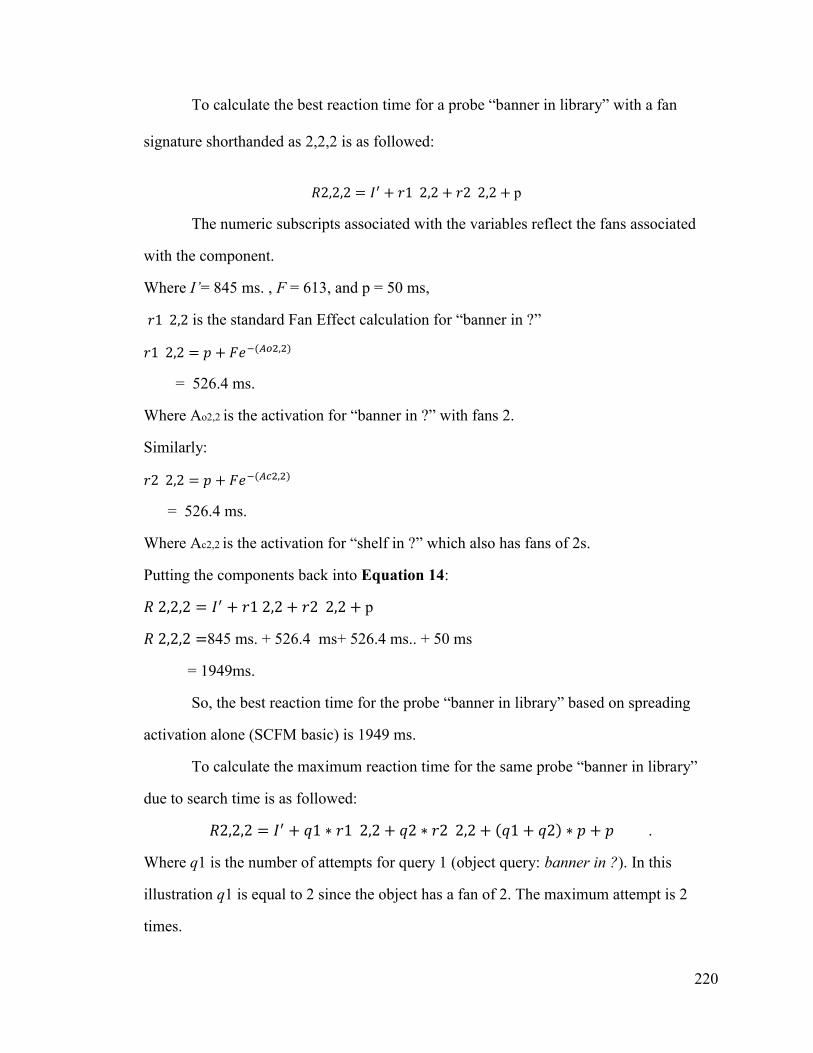
220

To calculate the best reaction time for a probe “banner in library” with a fan

signature shorthanded as 2,2,2 is as followed:

p

The numeric subscripts associated with the variables reflect the fans associated

with the component.

Where I’= 845 ms. , F = 613, and p = 50 ms,

is the standard Fan Effect calculation for “banner in ?”

)

= 526.4 ms.

Where Ao2,2 is the activation for “banner in ?” with fans 2.

Similarly:

)

= 526.4 ms.

Where Ac2,2 is the activation for “shelf in ?” which also has fans of 2s.

Putting the components back into Equation 14:

p

845 ms. + 526.4 ms+ 526.4 ms.. + 50 ms

= 1949ms.

So, the best reaction time for the probe “banner in library” based on spreading

activation alone (SCFM basic) is 1949 ms.

To calculate the maximum reaction time for the same probe “banner in library”

due to search time is as followed:

) .

Where q1 is the number of attempts for query 1 (object query: banner in ?). In this

illustration q1 is equal to 2 since the object has a fan of 2. The maximum attempt is 2

times.

221

Where q2 is the number of attempts for query 2 (container query: shelf in ?) in this

illustration q2 is equal to 1 since the container has a fan of 2 with one fan connecting to

“banner” the object and another fan for connecting to “library” and it only needs one

attempt to retrieve the right location “library”; “ )” is the factor for the additional

number of cognitive cycle added for the search productions - “ )*p” is the total

added cognitive cycle time for the search productions. And the last p in the equation is

the cognitive cycle time for the recognition production.

Using I’= 845 ms. , F = 613, and p = 50 ms, q1=2, q2=1,

is the standard Fan Effect calculation for “banner in ?”

)

= 526.4 ms.

Where Ao2 is the activation for “banner in ?” with fans 2. Similarly,

)

= 526.4 ms.

Where Ac2 is the activation for “shelf in library” also with fans 2.

) p

845 ms. + 2*526.4 ms+ 1*526.4 ms. + 150 ms+50 ms

= 2625ms.

So, the maximum reaction time for the probe “banner in library” based on SCFM

search model is 2625 ms.

Given the minimum (optimal) and maximum reaction times, one could venture to

calculate an average reaction time for the SCFM search model. One form of average

calculation is like the calculation of an average speed. The average is obtained by

summing the minimum and the maximum and dividing it by 2:

SCFM search 2,2,2 = (2625+1949)/2 = 2287 ms.

222

Appendix E ACT-R Simulation Models

This appendix contains the simulation codes for Experiments 1, 2 and 4. These

models are specified in terms of Python ACT-R syntax. The execution of these models

requires the ccm module for Python ACT-R and the CFlib module for the complex fan

functions.

E.1 Python ACT-R simulation model code for Experiments 1, 2 and 4

# Fan effect Simulation for exp 1,2,4

# Author: Kam Kwok, 2015

# status:

# Input files: exp_data.txt: 'item1 item2...', e.g.'object color', exp_probes.txt: e.g.'obj is

color'

# FanModel class defines Production rules, memory module used

# lib: CFlib, ccm, time, other libs

# output format: exp record format (csv): probe,ans,rt,f1,f2,date,mem mod; output: a .csv

file

''' FanTest 1) provides a UI, 2) creates the model(FanModel) as a child process, 3) env-to-

model commn: set run conditions,

provides child process commands to signal task done. FanModel is the fan act-r model.

'''

import ccm

from ccm.lib.actr import *

import CFlib

import time

from ccm.lib.actr.hdm import *

#****************

# Utilities

#****************

datafile= ""

probefile = ""

csvfile=""

ansO = None

ansL = None

ans=None

probes=[]

wd={}

fd=()

# I = 845 + p

I = 895

# the experiment

223

class FanTest(ccm.Model):

def start(self):

global fd,cont,probes,probefile,datafile,ans,ansO,ansL # fan-dictionary, container

# Experiment records

exprecs=[]

modelist=[]

trials=0

xlist=[]

rtlist=[]

targets=CFlib.openf2l(datafile)

if app.logf.get():

csvfile = app.e2.get().split(".")[0]+"_results.csv"

hdr=['probe','ans','type','error','RT','fan1','fan2','Total fan','product of

fans','predicted RT','date','mod']

self.fwl2csv(hdr,csvfile)

for item in probes:

frmt_rec=[]

value=None #Total RT

# run agent for each cue

for style in ['byobj','bycolor']:

t1=self.now()

# visual perception time:

yield 0.47

self.style=style

self.obj,self.color=item.split()[0],item.split()[2]

yield self.sayYes,self.sayNo

self.style=None

self.obj=None

self.color=None

## # motor time

## yield 0.21

# motor time for I = 845

yield 0.31

rt=self.now()-t1

if value is None: value=rt

else: value=(value+rt)/2

if style == 'byobj':

ansO = ans

## print "obj ",ans

else:

ansL = ans

## print "loc ",ans

ans = (ansO or ansL)

trials=trials+1

224

self.obj=None

self.color=None

try:

# fan1

fan1 = str(wd[item.split()[0]])

except:

fan1 = '1'

# fan3

try:

fan3 = str(wd[item.split()[2]])

except:

fan3='1'

# process type and ans

s_item = item.split()[0]+' '+item.split()[2]

if s_item in targets:

typ=1

if ans:

error=0

else:

error=1

else:

typ=0

if ans:

error=1

else:

error=0

# log answers

if app.logstatus.get():

log.CFRT_DM[item,str(value),ans]=value

# each trial: for no error

## if ans:

# for plotting

xlist.append(fan1+fan3)

rtlist.append(value)

# exp record format (csv): probe,rt,fo,fc,fl,date,probe#

# exprecs is a list of list

# probe

frmt_rec.append(item)

frmt_rec.append(ans)

frmt_rec.append(typ)

frmt_rec.append(error)

# RT, fan1, container,fan2, fan3

frmt_rec.append(value*1000)

try:

225

# fan1

f1=wd[item.split()[0]]

except:

f1='1'

frmt_rec.append(f1)

## # fan2

## try:

## frmt_rec.append(cont)

## frmt_rec.append(wd[cont])

## except:

## frmt_rec.append('1')

# fan3

try:

# fan3

f3=wd[item.split()[2]]

except:

f3='1'

frmt_rec.append(f3)

tf = int(f1)+int(f3)

frmt_rec.append(tf)

# product of fans

pf = int(f1)* int(f3)

frmt_rec.append(pf)

#prediction: I + rt , I= 845 + p

pRT=CFlib.calrt([item.split()[0],item.split()[2]],datafile)[1]+ I

frmt_rec.append(pRT)

# date

frmt_rec.append(time.ctime())

# id

frmt_rec.append(datafile)

exprecs.append(frmt_rec)

if app.logf.get():

self.fwl2csv(frmt_rec,csvfile)

#plotxy(x_in,y_in,sym = 'ro', xl='Total Fan',

if app.plot.get():

CFlib.plotxy(xlist,rtlist)

def sayYes(self):

global yescount, ans

yescount = yescount+ 1

ans=1

def sayNo(self):

global nocount, ans

nocount = nocount+ 1

226

ans=0

# for cf container

def sayCont(self,c):

global cont

cont = c

# 1)write a list to a csv file

def fwl2csv(self,ilist,ofn):

''' input: ilist = [1,2,a,b] and out-file name, output: a csv file'''

wf = open (ofn,'a')

for item in ilist:

if isinstance(item,str):

wf.write(item+',')

else:

wf.write(str(item)+',')

wf.write('\n')

wf.close()

# 2)write a list of lists to a csv file using fwl2csv

def fwll2csv(self,ilist,ofn):

for item in ilist:

self.fwl2csv(item,ofn)

# used by: App.run_exp

def run_trial():

#root.update()

global nocount, yescount, cont, probes, wd, fd, datafile, probefile

print 'No. of subjects: ',app.s_n.get()

fd={}

wd={}

datafile = app.e1.get()

## print "running trial, ...datafile: ",datafile

probefile = app.e2.get()

try:

probes =[l.strip() for l in open(probefile,'r').readlines()]

except:

print 'No probe file!',probefile

wd = CFlib.f2wd(datafile)

#fd is the fan dictionary: 'obj is loc':[fo,fc,fl]

for line in open(datafile,'r').readlines():

fd =CFlib.line2fdict(line.strip(),wd)

for t in range(1, app.s_n.get()+1):

nocount, yescount=0.0,0.0

env=FanTest()

if app.hdmv.get():

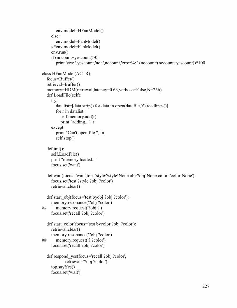
227

env.model=HFanModel()

else:

env.model=FanModel()

##env.model=FanModel()

env.run()

if (nocount+yescount)>0:

print 'yes: ',yescount,'no: ',nocount,'error%: ',(nocount/(nocount+yescount))*100

class HFanModel(ACTR):

focus=Buffer()

retrieval=Buffer()

memory=HDM(retrieval,latency=0.63,verbose=False,N=256)

def LoadFile(self):

try:

datalist=[data.strip() for data in open(datafile,'r').readlines()]

for r in datalist:

self.memory.add(r)

print "adding...", r

except:

print "Can't open file.", fn

self.stop()

def init():

self.LoadFile()

print "memory loaded..."

focus.set('wait')

def wait(focus='wait',top='style:?style!None obj:?obj!None color:?color!None'):

focus.set('test ?style ?obj ?color')

retrieval.clear()

def start_obj(focus='test byobj ?obj ?color'):

memory.resonance('?obj ?color')

## memory.request('?obj ?')

focus.set('recall ?obj ?color')

def start_color(focus='test bycolor ?obj ?color'):

retrieval.clear()

memory.resonance('?obj ?color')

## memory.request('? ?color')

focus.set('recall ?obj ?color')

def respond_yes(focus='recall ?obj ?color',

retrieval='?obj ?color'):

top.sayYes()

focus.set('wait')

228

def respond_no_obj(focus='recall ?obj ?color',

retrieval='? !?color'):

top.sayNo()

retrieval.clear()

focus.set('wait')

def respond_no_color(focus='recall ?obj ?color',

retrieval='!?obj ?'):

top.sayNo()

retrieval.clear()

focus.set('wait')

def respond_no_memerror(focus='recall ?obj ?color',

memory='error:True'):

top.sayNo()

retrieval.clear()

focus.set('wait')

class FanModel(ACTR):

global datafile

focus=Buffer()

retrieval=Buffer()

memory=Memory(retrieval,latency=0.63,threshold=-

25,maximum_time=20,finst_size=1000,finst_time=30000.0)

spread=DMSpreading(memory,focus)

spread.strength=1.6

spread.weight[focus]=0.5

def LoadFile(self):

try:

datalist=[data.strip() for data in open(datafile,'r').readlines()]

for r in datalist:

self.memory.add(r)

print "adding...", r

except:

print "Can't open file.", fn

self.stop()

def init():

self.LoadFile()

print "memory loaded..."

focus.set('wait')

def wait(focus='wait',top='style:?style!None obj:?obj!None color:?color!None'):

focus.set('test ?style ?obj ?color')

retrieval.clear()

def start_obj(focus='test byobj ?obj ?color'):

memory.request('?obj ?')

229

focus.set('recall ?obj ?color')

def start_color(focus='test bycolor ?obj ?color'):

retrieval.clear()

memory.request('? ?color')

focus.set('recall ?obj ?color')

def respond_yes(focus='recall ?obj ?color',

retrieval='?obj ?color'):

top.sayYes()

focus.set('wait')

def respond_no_obj(focus='recall ?obj ?color',

retrieval='? !?color'):

top.sayNo()

retrieval.clear()

focus.set('wait')

def respond_no_color(focus='recall ?obj ?color',

retrieval='!?obj ?'):

top.sayNo()

retrieval.clear()

focus.set('wait')

def respond_no_memerror(focus='recall ?obj ?color',

memory='error:True'):

top.sayNo()

retrieval.clear()

focus.set('wait')

#GUI and Main

from Tkinter import *

class App:

def __init__(self, master):

frame = Frame(master)

frame.pack()

self.plot = IntVar(value = 0)

self.opt_plot = Checkbutton(frame, text = "Plot RTs", variable=self.plot)

self.opt_plot.pack(side=RIGHT)

self.logf = IntVar(value = 0)

self.opt_logf = Checkbutton(frame, text = "Save csv file", variable=self.logf)

self.opt_logf.pack(side=RIGHT)

self.logstatus = IntVar(value = 1)

self.opt_logstatus = Checkbutton(frame, text = "Log trials", variable=self.logstatus)

self.opt_logstatus.pack(side=RIGHT)

self.hdmv = IntVar(value = 0)

self.hdm = Checkbutton(frame, text = "HDM model", variable=self.hdmv)

230

self.hdm.pack(side=RIGHT)

self.s_n = IntVar(value = 1)

self.ss_n = Scale(frame, label = 'No. of subjects:', variable=self.s_n,

from_=1, to=50, tickinterval=24, orient='horizontal')

self.ss_n.pack(side=RIGHT)

self.b_run = Button(frame, text="Run Experiment",

fg='red',command=self.run_exp)

self.b_run.pack(side=LEFT)

self.l1 = Label(text="data file:")

self.l1.pack( side = LEFT)

self.dataf = StringVar()

self.dataf.set("exp2_targets.txt")

self.e1 = Entry(bd =5,textvariable=self.dataf)

self.e1.pack(side = LEFT)

self.l2 = Label(text="probes file:")

self.l2.pack( side = LEFT)

self.probef = StringVar()

self.probef.set("exp2_probes.txt")

self.e2 = Entry(bd =5,textvariable=self.probef)

self.e2.pack(side = LEFT)

# This is a handler for the run button - running the experiment

def run_exp(self):

run_trial()

# experiment init

ans=True

log=ccm.log()

##fd={}

##try:

## probes =[l.strip() for l is open(probefile,'r').readlines()]

##except:

## print 'No probe file!'

##

##wd = CFlib.f2wd(datafile)

###fd is the fan dictionary: 'obj is loc':[fo,fc,fl]

##for line is open(datafile,'r').readlines():

## fd =CFlib.line2fdict(line.strip(),wd)

root = Tk(className=" Fan Fffect Simulation")

app = App(root)

root.mainloop()

231

E.2 Python ACT-R simulation model code for Experiment 3 (SCFM basic model)

# Complex Fan - SCFM basic model (no search)

# Author: Kam Kwok, 2015

# status: work in progress

# What's new: fixed ans. added retry as in hdm_inhibit; added HDM option;

# Input files: exp_data.txt: 'item1 item2...', e.g.'object container', exp_probes.txt: e.g.'obj

in location'

# FanModel/HdmModel class defines Production rules, memory module used

# lib: CFlib, ccm, time, other libs

# output format: exp record format (csv):

# 'probe','ans','type','error','RT','fan1','container','fanc','fan3','date','mod'

''' FanTest 1) provides a UI, 2) creates the model(FanModel) as a child process, 3) env-to-

model commn: set run conditions,

provides child process commands to signal task done. FanModel is the fan act-r model.

'''

import ccm

from ccm.lib.actr import *

import CFlib

import time

from ccm.lib.actr.hdm import *

#****************

# Utilities

#****************

datafile= ""

probefile = ""

csvfile=""

ansO = None

ansL = None

ans=None

probes=[]

wd={}

fd=()

class FanModel(ACTR):

global datafile

focus=Buffer()

retrieval=Buffer()

memory=Memory(retrieval,latency=0.63,threshold=-

25,maximum_time=20,finst_size=1000,finst_time=30000.0)

spread=DMSpreading(memory,focus)

spread.strength=1.6

spread.weight[focus]=0.5

def LoadFile(self):

try:

datalist=[data.strip() for data in open(datafile,'r').readlines()]

232

for r in datalist:

self.memory.add(r)

## print "adding...", r

except:

print "Can't open file.", fn

self.stop()

def init():

global verbose

self.LoadFile()

print "memory loaded..."

focus.set('wait')

def wait(focus='wait',top='style:?style!None obj:?obj!None location:?location!None'):

focus.set('test ?style ?obj ?location')

retrieval.clear()

def start_objRqst(focus='test byobj ?obj ?location'):

memory.request('?obj ?')

print "start_objRqst with object: ",obj

focus.set('queryoc ?obj ?location')

def No_obj_cont(focus='queryoc ?obj ?location',

memory='error:True'):

top.sayNo()

retrieval.clear()

focus.set('wait')

def containerRqst(focus='queryoc ?obj ?location',memory='busy:False',

retrieval='?obj ?container'):

retrieval.clear()

memory.request('?container ?')

print "containerRqst with container: ",container

focus.set('compCL ?obj ?location')

def compCLYes(focus='compCL ?obj ?location',memory='busy:False',

retrieval='?container ?location'):

top.sayYes()

top.sayCont(container)

retrieval.clear()

print "Yes Conirmation: ",obj," in ",location

focus.set('wait')

def No_cont_loc(focus='compCL ?obj ?location',

233

memory='error:True'):

print "No, memory error!"

top.sayNo()

## retrieval.clear()

focus.set('wait')

## focus.set('retry ?obj ?location')

def respond_no_CL(focus='compCL ?obj ?location',

retrieval='?container !?location'):

print "No, wrong location: ", location

top.sayNo()

retrieval.clear()

focus.set('wait')

class FanTest(ccm.Model):

def start(self):

global fd,cont,probes,probefile,ans,ansO,ansL # fan-dictionary, container

# Experiment records

exprecs=[]

trials=0

xlist=[]

rtlist=[]

targets=CFlib.openf2l(app.e4.get())

csvfile=app.e3.get()

if app.logf.get():

hdr=['probe','ans','type','error','RT','fan1','container','fanC',

'fan3','date','mod']

self.fwl2csv(hdr,csvfile)

for item in probes:

frmt_rec=[]

value=None #Total RT

# run agent for each cue

## for style in ['byobj','byloc']:

for style in ['byobj']:

t1=self.now()

# visual perception time:

#yield 0.47

self.style=style

self.obj,cont,self.location=item.split()[0],None,item.split()[2]

yield self.sayYes,self.sayNo

# motor time

#yield 0.21

rt=self.now()-t1

yt = 0.68

234

if value is None: value=rt+yt

else: value=(value+rt+yt)/2

if style == 'byobj':

ansO = ans

## print "obj ",ans

else:

ansL = ans

## print "loc ",ans

## ans = (ansO or ansL)

ans = (ansO)

trials=trials+1

self.obj=None

self.location=None

try:

# fan1

fan1 = wd[item.split()[0]]

except:

fan1 = '1'

# fanIn/ fan container

try:

fanc = wd[cont]

except:

fanc ='1'

# fan3

try:

fan3 = wd[item.split()[2]]

except:

fan3='1'

# process type and ans

s_item = item.split()[0]+' '+item.split()[2]

if s_item in targets:

typ=1

if ans:

error=0

else:

error=1

else:

typ=0

if ans:

error=1

else:

error=0

# log answers

if app.logstatus.get():

log.CFRT_DM[item,str(value),ans]=value

## if app.hdmv.get():

235

## log.CFRT_HDM[item,str(value),ans]=value

## else:

# each trial: for no error

# for plotting

#print "fan...",fan1+fanc+fan3

#totalf = fan1+fanc+fan3

if error == 0:

xlist.append(trials)

rtlist.append(value)

# exp record format (csv): probe,rt,fo,fc,fl,date,probe#

# exprecs is a list of list

# probe

frmt_rec.append(item)

frmt_rec.append(ans)

frmt_rec.append(typ)

frmt_rec.append(error)

# RT, fan1, container,fan2, fan3

frmt_rec.append(value)

try:

# fan1

frmt_rec.append(wd[item.split()[0]])

except:

frmt_rec.append('1')

# fanc

try:

frmt_rec.append(cont)

frmt_rec.append(wd[cont])

except:

frmt_rec.append('1')

# fan3

try:

frmt_rec.append(wd[item.split()[2]])

except:

frmt_rec.append('1')

# date

frmt_rec.append(time.ctime())

# id

frmt_rec.append(datafile)

exprecs.append(frmt_rec)

if app.logf.get():

self.fwl2csv(frmt_rec,csvfile)

#plotxy(x_in,y_in,sym = 'ro', xl='Total Fan',

236

if app.plot.get():

CFlib.plotxy(xlist,rtlist)

def sayYes(self):

global yescount, ans

yescount = yescount+ 1

ans=1

def sayNo(self):

global nocount, ans

nocount = nocount+ 1

ans=0

# for cf container

def sayCont(self,c):

global cont

cont = c

# 1)write a list to a csv file

def fwl2csv(self,ilist,ofn):

''' input: ilist = [1,2,a,b] and out-file name, output: a csv file'''

wf = open (ofn,'a')

for item in ilist:

if isinstance(item,str):

wf.write(item+',')

else:

wf.write(str(item)+',')

wf.write('\n')

wf.close()

# 2)write a list of lists to a csv file using fwl2csv

def fwll2csv(self,ilist,ofn):

for item in ilist:

self.fwl2csv(item,ofn)

# used by: App.run_exp

def run_trial():

#root.update()

global nocount, yescount, cont, probes, wd, fd, datafile, probefile

print 'No. of subjects: ',app.s_n.get()

fd={}

datafile = app.e1.get()

## print "running trial, ...datafile: ",datafile

probefile = app.e2.get()

try:

237

probes =[l.strip() for l in open(probefile,'r').readlines()]

except:

print 'No probe file!',probefile

wd = CFlib.f2wd(datafile)

#fd is the fan dictionary: 'obj is loc':[fo,fc,fl]

for line in open(datafile,'r').readlines():

fd =CFlib.line2fdict(line.strip(),wd)

for t in range(1, app.s_n.get()+1):

nocount, yescount=0.0,0.0

env=FanTest()

## if app.hdmv.get():

## env.model=HdmModel()

## else:

env.model=FanModel()

env.run()

if (nocount+yescount)>0:

print 'yes: ',yescount,'no: ',nocount,'error%: ',(nocount/(nocount+yescount))*100

#GUI and Main

from Tkinter import *

class App:

def __init__(self, master):

frame = Frame(master)

frame.pack()

self.plot = IntVar(value = 0)

self.opt_plot = Checkbutton(frame, text = "Plot RTs", variable=self.plot)

self.opt_plot.pack(side=RIGHT)

self.logf = IntVar(value = 0)

self.opt_logf = Checkbutton(frame, text = "Save csv file", variable=self.logf)

self.opt_logf.pack(side=RIGHT)

self.logstatus = IntVar(value = 1)

self.opt_logstatus = Checkbutton(frame, text = "Log trials", variable=self.logstatus)

self.opt_logstatus.pack(side=RIGHT)

## self.hdmv = IntVar(value = 0)

## self.hdm = Checkbutton(frame, text = "HDM model", variable=self.hdmv)

## self.hdm.pack(side=RIGHT)

self.s_n = IntVar(value = 1)

self.ss_n = Scale(frame, label = 'No. of subjects:', variable=self.s_n,

from_=1, to=50, tickinterval=24, orient='horizontal')

self.ss_n.pack(side=RIGHT)

self.b_run = Button(frame, text="Run Experiment",

fg='red',command=self.run_exp)

self.b_run.pack(side=LEFT)

self.l1 = Label(text="data file:")

self.l1.pack( side = LEFT)

238

self.dataf = StringVar()

self.dataf.set("exp3_targets.txt")

self.e1 = Entry(bd =5,textvariable=self.dataf)

self.e1.pack(side = LEFT)

self.l2 = Label(text="probes file:")

self.l2.pack( side = LEFT)

self.probef = StringVar()

self.probef.set("exp3_probes.txt")

self.e2 = Entry(bd =5,textvariable=self.probef)

self.e2.pack(side = LEFT)

self.csvf = StringVar()

self.csvf.set("SCFMresults.csv")

self.l3 = Label(text="csv file:")

self.l3.pack( side = LEFT)

self.e3 = Entry(bd =5,textvariable=self.csvf)

self.e3.pack(side = LEFT)

self.targetf = StringVar()

self.targetf.set("exp3_targets.txt")

self.l4 = Label(text="target file:")

self.l4.pack( side = LEFT)

self.e4 = Entry(bd =5,textvariable=self.targetf)

self.e4.pack(side = LEFT)

# This is a handler for the run button - running the experiment

def run_exp(self):

run_trial()

# experiment init

log=ccm.log()

root = Tk(className=" Complex Fan Effect Simulation")

app = App(root)

root.mainloop()

239

E.3 Python ACT-R simulation model code for Experiment 3 (SCFM with search)

# Complex Fan - SCFM serach Simulation for Experiment 3

# HDM model included

# Author: Kam Kwok, 2015

# status: work in progress

# What's new: fixed ans. added retry as in hdm_inhibit; added HDM option;

# Input files: exp_data.txt: 'item1 item2...', e.g.'object container', exp_probes.txt: e.g.'obj

in location'

# FanModel/HdmModel class defines Production rules, memory module used

# lib: CFlib, ccm, time, other libs

# output format: exp record format (csv):

# 'probe','ans','type','error','RT','fan1','container','fanc','fan3','date','mod'

''' FanTest 1) provides a UI, 2) creates the model(FanModel) as a child process,

3) env-to-model commn: set run conditions,

provides child process commands to signal task done. FanModel is the fan act-r model.

'''

import ccm

from ccm.lib.actr import *

import CFlib

import time

from ccm.lib.actr.hdm import *

#****************

# Utilities

#****************

datafile= ""

probefile = ""

csvfile=""

ansO = None

ansL = None

ans=None

probes=[]

wd={}

fd=()

class FanModel(ACTR):

global datafile

focus=Buffer()

retrieval=Buffer()

memory=Memory(retrieval,latency=0.63,threshold=-

25,maximum_time=20,finst_size=1000,finst_time=30000.0)

spread=DMSpreading(memory,focus)

spread.strength=1.6

spread.weight[focus]=0.5

def LoadFile(self):

try:

240

datalist=[data.strip() for data in open(datafile,'r').readlines()]

for r in datalist:

self.memory.add(r)

## print "adding...", r

except:

print "Can't open file.", fn

self.stop()

def init():

global verbose

self.LoadFile()

print "SCFM with search: memory loaded..."

focus.set('wait')

def wait(focus='wait',top='style:?style!None obj:?obj!None location:?location!None'):

focus.set('test ?style ?obj ?location')

retrieval.clear()

def start_objRqst(focus='test byobj ?obj ?location'):

memory.request('?obj ?')

print "start_objRqst with object: ",obj

focus.set('queryoc ?obj ?location')

def No_obj_cont(focus='queryoc ?obj ?location',

memory='error:True'):

top.sayNo()

retrieval.clear()

focus.set('wait')

def containerRqst(focus='queryoc ?obj ?location',memory='busy:False',

retrieval='?obj ?container'):

retrieval.clear()

memory.request('?container ?')

print "containerRqst with container: ",container

focus.set('compCL ?obj ?location')

def compCLYes(focus='compCL ?obj ?location',memory='busy:False',

retrieval='?container ?location'):

top.sayYes()

top.sayCont(container)

retrieval.clear()

print "Yes confirmation: ",obj," in ",location

focus.set('wait')

241

def No_cont_loc(focus='compCL ?obj ?location',

memory='error:True'):

print "Retrieval failed; goto retry "

## top.sayNo()

retrieval.clear()

focus.set('retry ?obj ?location')

## def respond_no_CL(focus='compCL ?obj ?location',

## retrieval='?container !?location'):

## print "No, Diff loc. say false.", location

## top.sayNo()

## retrieval.clear()

## focus.set('wait')

# retry update

def retry_no_CL(focus='compCL ?obj ?location',

retrieval='?container !?location'):

retrieval.clear()

print "Wrong location goto retry ", location

focus.set('retry ?obj ?location')

def retry_newc(focus='retry ?obj ?location'):

retrieval.clear()

memory.request('?obj ?',require_new=True)

print "New containerRqst... "

focus.set('retryl ?obj ?location')

def No_2cont(focus='retryl ?obj ?location',

memory='error:True'):

top.sayNo()

retrieval.clear()

top.sayNo()

print "No confirmation; no more container."

retrieval.clear()

focus.set('wait')

def retry_with_c2(focus='retryl ?obj ?location',memory='busy:False',

retrieval='?obj ?container2'):

retrieval.clear()

memory.request('?container2 ?')

print "Retry with container(2): ",container2

focus.set('rcomp ?obj ?location')

def retry_yes(focus='rcomp ?obj ?location',

retrieval='?container2 ?location'):

242

top.sayYes()

top.sayCont(container2)

print "Yes confirmation: ",obj," in ",container2," in ",location

retrieval.clear()

focus.set('wait')

def retry_wrong_loc(focus='rcomp ?obj ?location',

retrieval='?container2 !?location'):

top.sayNo()

print "No confirmation; wrong location with retry"

retrieval.clear()

focus.set('wait')

def retry_noloc(focus='rcomp ?obj ?location',

memory='error:True'):

top.sayNo()

print "No confirmation; memory error with retry"

retrieval.clear()

focus.set('wait')

# retry update ends

## byloc

def start_loc(focus='test byloc ?obj ?location'):

memory.request('? ?location')

print "byloc...loc ",location

focus.set('querycl ?obj ?location')

def OCRqst(focus='querycl ?obj ?location',memory='busy:False',

retrieval='?container ?location'):

retrieval.clear()

memory.request('? ?container')

print "byloc...container... ",container

focus.set('compOC ?obj ?location')

def compOCYes(focus='compOC ?obj ?location',

retrieval='?obj ?container'):

top.sayYes()

print "byloc...right obj container",obj, container

top.sayCont(container)

retrieval.clear()

focus.set('wait')

def compOCerrorNo(focus='compOC ?obj ?location',

243

memory='error:True'):

print "byloc...No, error, no obj..."

top.sayNo()

retrieval.clear()

focus.set('wait')

def respond_no_OC(focus='compOC ?obj ?location',

retrieval='!?obj ?container'):

print "byloc...No, wrong obj...", obj

top.sayNo()

retrieval.clear()

focus.set('wait')

class HdmModel(ACTR):

global datafile

focus=Buffer()

retrieval=Buffer()

memory=HDM(retrieval,latency=0.63,verbose=False,N=256)

def LoadFile(self):

try:

datalist=[data.strip() for data in open(datafile,'r').readlines()]

for r in datalist:

self.memory.add(r)

## print "adding...", r

except:

print "Can't open file.", fn

self.stop()

def init():

self.LoadFile()

print "memory loaded..."

focus.set('wait')

def wait(focus='wait',top='style:?style!None obj:?obj!None location:?location!None'):

focus.set('test ?style ?obj ?location')

retrieval.clear()

def start_objRqst(focus='test byobj ?obj ?location'):

memory.request('?obj ?')

print "start_objRqst...obj ",obj

focus.set('queryoc ?obj ?location')

def No_obj_cont(focus='queryoc ?obj ?location',

244

memory='error:True'):

top.sayNo()

retrieval.clear()

focus.set('wait')

def containerRqst(focus='queryoc ?obj ?location',memory='busy:False',

retrieval='?obj ?container'):

retrieval.clear()

memory.request('?container ?')

print "containerRqst...container ",container

focus.set('compCL ?obj ?location')

def compCLYes(focus='compCL ?obj ?location',memory='busy:False',

retrieval='?container ?location'):

print "right container-location ",container,location

top.sayYes()

top.sayCont(container)

retrieval.clear()

print "Yes, loc: ",location

focus.set('wait')

def No_cont_loc(focus='compCL ?obj ?location',

memory='error:True'):

print "No, memory error goto retry "

top.sayNo()

retrieval.clear()

focus.set('retry ?obj ?location')

# retry update

def retry_no_CL(focus='compCL ?obj ?location',

retrieval='?container !?location'):

retrieval.clear()

print "diff loc goto retry ", location

### DM change for HDM

focus.set('retry ?obj ?container ?location')

def retry_newc(focus='retry ?obj ?container ?location'):

retrieval.clear()

### DM change for HDM

## memory.request('?obj ?',require_new=True)

memory.request('?obj ?unknown!?container')

print "New containerRqst... "

focus.set('retryl ?obj ?location')

245

def No_2cont(focus='retryl ?obj ?location',

memory='error:True'):

top.sayNo()

retrieval.clear()

print "No cont2"

top.sayNo()

retrieval.clear()

focus.set('wait')

def retry_with_c2(focus='retryl ?obj ?location',memory='busy:False',

retrieval='?obj ?container2'):

retrieval.clear()

### DM change for HDM

## memory.request('?container2 ?')

memory.resonance('?container2 ?location')

print "container 2 ",container2

focus.set('rcomp ?obj ?location')

def retry_yes(focus='rcomp ?obj ?location',

retrieval='?container2 ?location'):

print "Yes, right container-loc ",container2,location

top.sayYes()

top.sayCont(container2)

retrieval.clear()

focus.set('wait')

def retry_wrong_loc(focus='rcomp ?obj ?location',

retrieval='?container2 !?location'):

print "No, cont2 gets wrong loc"

top.sayNo()

retrieval.clear()

focus.set('wait')

def retry_noloc(focus='rcomp ?obj ?location',

memory='error:True'):

print "No, mem error with cont2"

top.sayNo()

retrieval.clear()

focus.set('wait')

# retry update ends

## byloc

def start_loc(focus='test byloc ?obj ?location'):

memory.request('? ?location')

246

print "byloc...loc ",location

focus.set('querycl ?obj ?location')

def OCRqst(focus='querycl ?obj ?location',memory='busy:False',

retrieval='?container ?location'):

retrieval.clear()

### DM change for HDM

## memory.request('? ?container')

memory.resonance('?obj ?container')

print "byloc...container... ",container

focus.set('compOC ?obj ?location')

def compOCYes(focus='compOC ?obj ?location',

retrieval='?obj ?container'):

top.sayYes()

print "byloc...right obj container",obj, container

top.sayCont(container)

retrieval.clear()

focus.set('wait')

def compOCerrorNo(focus='compOC ?obj ?location',

memory='error:True'):

print "byloc...No, error, no obj..."

top.sayNo()

retrieval.clear()

focus.set('wait')

def respond_no_OC(focus='compOC ?obj ?location',

retrieval='!?obj ?container'):

print "byloc...No, wrong obj...", obj

top.sayNo()

retrieval.clear()

focus.set('wait')

# The experiment for one participant

class FanTest(ccm.Model):

def start(self):

global fd,cont,probes,probefile,ans,ansO,ansL # fan-dictionary, container

# Experiment records

exprecs=[]

trials=0

xlist=[]

247

rtlist=[]

targets=CFlib.openf2l(app.e4.get())

csvfile=app.e3.get()

if app.logf.get():

hdr=['probe','ans','type','error','RT','fan1','container','fanC',

'fan3','date','mod']

self.fwl2csv(hdr,csvfile)

for item in probes:

frmt_rec=[]

value=None #Total RT

# run agent for each cue

## for style in ['byobj','byloc']:

for style in ['byobj']:

t1=self.now()

# visual perception time:

#yield 0.47

self.style=style

self.obj,cont,self.location=item.split()[0],None,item.split()[2]

yield self.sayYes,self.sayNo

# motor time

#yield 0.21

rt=self.now()-t1

## yt = 0.68

# I = 845

yt = 0.78

if value is None: value=rt+yt

else: value=(value+rt+yt)/2

if style == 'byobj':

ansO = ans

## print "obj ",ans

else:

ansL = ans

## print "loc ",ans

## ans = (ansO or ansL)

value = value * 1000

trials=trials+1

self.obj=None

self.location=None

try:

# fan1

fan1 = wd[item.split()[0]]

except:

fan1 = '1'

# fanIn/ fan container

try:

248

fanc = wd[cont]

except:

fanc ='1'

# fan3

try:

fan3 = wd[item.split()[2]]

except:

fan3='1'

# process type and ans

s_item = item.split()[0]+' '+item.split()[2]

if s_item in targets:

typ=1

if ans:

error=0

else:

error=1

else:

typ=0

if ans:

error=1

else:

error=0

# log answers

if app.logstatus.get():

if app.hdmv.get():

log.CFRT_HDM[item,str(value),ans]=value

else:

log.CFRT_DM[item,str(value),ans]=value

# each trial: for no error

# for plotting

#print "fan...",fan1+fanc+fan3

#totalf = fan1+fanc+fan3

if error == 0:

xlist.append(trials)

rtlist.append(value)

# exp record format (csv): probe,rt,fo,fc,fl,date,probe#

# exprecs is a list of list

# probe

frmt_rec.append(item)

frmt_rec.append(ans)

frmt_rec.append(typ)

frmt_rec.append(error)

# RT, fan1, container,fan2, fan3

frmt_rec.append(value)

249

try:

# fan1

frmt_rec.append(wd[item.split()[0]])

except:

frmt_rec.append('1')

# fanc

try:

frmt_rec.append(cont)

frmt_rec.append(wd[cont])

except:

frmt_rec.append('1')

# fan3

try:

frmt_rec.append(wd[item.split()[2]])

except:

frmt_rec.append('1')

# date

frmt_rec.append(time.ctime())

# id

frmt_rec.append(datafile)

exprecs.append(frmt_rec)

if app.logf.get():

self.fwl2csv(frmt_rec,csvfile)

#plotxy(x_in,y_in,sym = 'ro', xl='Total Fan',

if app.plot.get():

CFlib.plotxy(xlist,rtlist)

def sayYes(self):

global yescount, ans

yescount = yescount+ 1

ans=1

def sayNo(self):

global nocount, ans

nocount = nocount+ 1

ans=0

# for cf container

def sayCont(self,c):

global cont

cont = c

# 1)write a list to a csv file

def fwl2csv(self,ilist,ofn):

250

''' input: ilist = [1,2,a,b] and out-file name, output: a csv file'''

wf = open (ofn,'a')

for item in ilist:

if isinstance(item,str):

wf.write(item+',')

else:

wf.write(str(item)+',')

wf.write('\n')

wf.close()

# 2)write a list of lists to a csv file using fwl2csv

def fwll2csv(self,ilist,ofn):

for item in ilist:

self.fwl2csv(item,ofn)

# used by: App.run_exp

def run_trial():

#root.update()

global nocount, yescount, cont, probes, wd, fd, datafile, probefile

print 'No. of subjects: ',app.s_n.get()

fd={}

wd={}

datafile = app.e1.get()

## print "running trial, ...datafile: ",datafile

probefile = app.e2.get()

try:

probes =[l.strip() for l in open(probefile,'r').readlines()]

except:

print 'No probe file!',probefile

wd = CFlib.f2wd(datafile)

#fd is the fan dictionary: 'obj is loc':[fo,fc,fl]

for line in open(datafile,'r').readlines():

fd =CFlib.line2fdict(line.strip(),wd)

for t in range(1, app.s_n.get()+1):

nocount, yescount=0.0,0.0

env=FanTest()

if app.hdmv.get():

env.model=HdmModel()

else:

env.model=FanModel()

env.run()

if (nocount+yescount)>0:

print 'yes: ',yescount,'no: ',nocount,'error%: ',(nocount/(nocount+yescount))*100

#GUI and Main

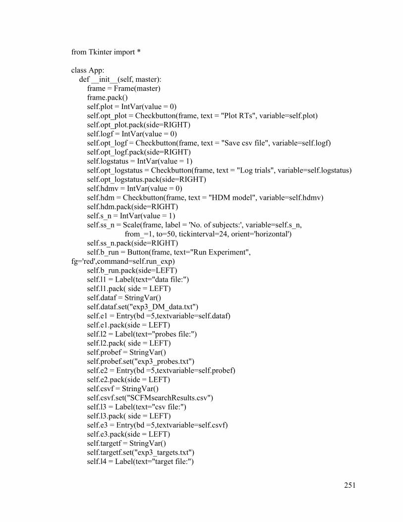
251

from Tkinter import *

class App:

def __init__(self, master):

frame = Frame(master)

frame.pack()

self.plot = IntVar(value = 0)

self.opt_plot = Checkbutton(frame, text = "Plot RTs", variable=self.plot)

self.opt_plot.pack(side=RIGHT)

self.logf = IntVar(value = 0)

self.opt_logf = Checkbutton(frame, text = "Save csv file", variable=self.logf)

self.opt_logf.pack(side=RIGHT)

self.logstatus = IntVar(value = 1)

self.opt_logstatus = Checkbutton(frame, text = "Log trials", variable=self.logstatus)

self.opt_logstatus.pack(side=RIGHT)

self.hdmv = IntVar(value = 0)

self.hdm = Checkbutton(frame, text = "HDM model", variable=self.hdmv)

self.hdm.pack(side=RIGHT)

self.s_n = IntVar(value = 1)

self.ss_n = Scale(frame, label = 'No. of subjects:', variable=self.s_n,

from_=1, to=50, tickinterval=24, orient='horizontal')

self.ss_n.pack(side=RIGHT)

self.b_run = Button(frame, text="Run Experiment",

fg='red',command=self.run_exp)

self.b_run.pack(side=LEFT)

self.l1 = Label(text="data file:")

self.l1.pack( side = LEFT)

self.dataf = StringVar()

self.dataf.set("exp3_DM_data.txt")

self.e1 = Entry(bd =5,textvariable=self.dataf)

self.e1.pack(side = LEFT)

self.l2 = Label(text="probes file:")

self.l2.pack( side = LEFT)

self.probef = StringVar()

self.probef.set("exp3_probes.txt")

self.e2 = Entry(bd =5,textvariable=self.probef)

self.e2.pack(side = LEFT)

self.csvf = StringVar()

self.csvf.set("SCFMsearchResults.csv")

self.l3 = Label(text="csv file:")

self.l3.pack( side = LEFT)

self.e3 = Entry(bd =5,textvariable=self.csvf)

self.e3.pack(side = LEFT)

self.targetf = StringVar()

self.targetf.set("exp3_targets.txt")

self.l4 = Label(text="target file:")

252

self.l4.pack( side = LEFT)

self.e4 = Entry(bd =5,textvariable=self.targetf)

self.e4.pack(side = LEFT)

# This is a handler for the run button - running the experiment

def run_exp(self):

run_trial()

# experiment init

log=ccm.log()

root = Tk(className=" Complex Fan Effect Simulation")

app = App(root)

root.mainloop()

253

Appendix F Experiment Apparatus

This appendix contains the Python codes for apparatus used in Experiments 1, 2

and 4. The execution of these apparatus requires the support of Python 2.7 or higher

support. The design of the apparatus is documented in the embedded comments.

F.1 OCLearn module

# Complex Fan experiment apparatus OCLearn module Version 1.0

# For learning and qualifying tests for experiment 1,2, 4

# Inputs: objcont.txt, objcontprb.txt (targets+foils); contloc.txt, contlocprb.txt, cftargets,

cfprobes.txt

# Output: <userid>.csv with headers

# Flow: 1.study targets, 2.recall training > 80%, 3. if qualify test > 90% -> 4. experiment

# Author: Kam Kwok ,2014

from Tkinter import *

import tkMessageBox

import tkFileDialog

import random

import time

#globals -------------------->

#fact list from file

gfactlst = []

#sublst

sublst=[]

#My dialog answer or e3_get/eText.get()

ans = ''

#My dialog user name

user =''

# user study + test time records (list)

lrntsttime=0

# targets count

tcount=0

# session percents

lpc=0

qpc=0

#learn file targets file name set by study_test()

fname=''

#word count dictionary

wd={}

#fan count dictionary

fd={}

254

# facts per learn segment constant

fps=3

#globals <--------------------!

anslist=[]

# input dialog class; return ans as a global

# bind <return> to method send

class MyDialog:

def __init__(self, parent, fact):

top = self.top = Toplevel(parent)

w, h = self.top.winfo_screenwidth(), self.top.winfo_screenheight()

self.top.geometry('260x260+%d+%d' % (w/2, h/2))

self.myLabel = Label(top, text= fact)

self.myLabel.pack()

self.myEntryBox = Entry(top)

self.myEntryBox.pack()

self.mySubmitButton = Button(top, text='Submit', command=self.send)

self.mySubmitButton.pack()

self.myEntryBox.bind('<Return>',self.send)

self.myEntryBox.focus()

def send(self,key='<Return>'):

global ans

ans = self.myEntryBox.get()

self.top.destroy()

#add to a word count dictionary from a string

def wdict(inline):

global wd

sequence = inline.split()

for x in sequence:

if wd.has_key(x):

wd[x] += 1

else:

wd[x] = 1

# add to fan dictionary {'chunk':(f1,f2,f3)} record

# input: wd and a string;

# return a tuple and update in fd

def fdict(inline):

global fd,wd

ft=[]

255

rs=''

inline=inline.strip()

sequence = inline.split()

for x in sequence:

if wd.has_key(x):

ft.append (wd[x])

rs=rs+str (wd[x])+','

else:

ft.append (0)

rs=rs+str ('0,')

fd[inline]=ft

return (rs)

# read a file to set global fact list (gfactlst)

def openDataFile():

global gfactlst,fname

f = tkFileDialog.askopenfile(parent=tk,mode='r',title='Choose a file',

filetypes=[('text files', '.txt')])

if f :

fname=f.name

l = f.readlines()

f.close

gfactlst = [str.strip(line) for line in l]

display(gfactlst)

# read a file into global var gfactlst

def openf(fs):

global gfactlst, fname

fname=fs

f = open(fs,'r')

l = f.readlines()

f.close

gfactlst = [str.strip(line) for line in l]

#File to list; Called by Qtest for targets

def openf2l(fs):

f = open(fs,'r')

l = f.readlines()

f.close

return ([str.strip(line) for line in l])

# Base subr for all studies

# Called by savelrn

def app2csv(usr, rStr):

session = open(usr+'.csv', 'a')

256

session.write(rStr)

session.close()

#l2txt.set("A user record is saved")

def addrec(fs=user,lst=['Probe','Type','Answer','Reaction

time','Error','fan1','fanIn','fan2','Date/time',fname]):

savrec = ','.join(lst)+'\n'

app2csv(fs, savrec)

# Called by Qtest (after each study-test > 90%)

def savelrn():

global tcount,lpc,qpc,lrntsttime, fname

headr =['user','fname','learn percent','Qtest percent','Target count','Total learn

time',str(time.ctime())]

savrec = ','.join(headr)+'\n'

app2csv(user, savrec)

usrrec =[user,fname,str(lpc),str(qpc),str(tcount), str(lrntsttime)]

savrec = ','.join(usrrec)+'\n'

app2csv(user, savrec)

lpc =0

tcount=0

lrntsttime=0

qpc=0

# Called by lrn

# study and test sublists

def study_test(fs):

global gfactlst, lrntsttime, sublst,lpc, fname, fps

fname=fs

openf(fs)

if len(gfactlst) == 0:

# ask for data file name and load it into gfactlst

openDataFile()

#create a work copy

wblst = gfactlst[:]

#create a list of sublists

sublists=[wblst[i:i+fps] for i in range(0, len(wblst), fps)]# start, stop, step

#Record start time

startT= time.time()

while sublists:

y = sublists.pop()

if len(y)==0: continue

# z is a copy of a sublist for testing

z = y[:]

sublst= y[:]

while y:

257

x =y.pop()

l1txt.set(x)

tk.update()

time.sleep(4)

l1txt.set('')

tk.update()

#start fill-in-the-blanks

pc=pretestlist(z)

# loop with sublist until > 80%

while pc < 80:

z=sublst[:]

pc = pretestlist(z)

#record learn percent

# record learning time

lpc=pc

l1txt.set('')

#Called by study-test

#Need a sublist as input;

def pretestlist(wblst):

tcount = len(wblst)

#if tcount ==0: return 0

count =0

# create reference list copied from worklist/sublist

refl= wblst[:]

msg="'Recall Training'; you must achieve > 80% to progress to the next set."

tkMessageBox.showinfo("Recall Trainning",msg)

random.shuffle(wblst)

while wblst:

x = wblst.pop()

if x == '': continue

lastword = x.split()[-1]

firstPart = ' '.join(x.split()[0:2])

q = firstPart + ' _____?'

tk.title("Recall Training")

inputDialog = MyDialog(tk,q)

tk.wait_window(inputDialog.top)

# submission is in ans

answer = firstPart+' '+ ans

if ans == lastword:

if answer in refl:

refl.remove(answer)

count = count +1

l1txt.set('Correct!')

#refl.remove(answer)

else:

258

# check if it is the other answers

if answer in refl:

l1txt.set('Correct')

count = count +1

refl.remove(answer)

#wblst.append(x)

else:

msg = "Sorry! The ans is: "+x

l1txt.set(msg)

tkMessageBox.showinfo("The Answer",msg)

l1txt.set('')

tk.update()

pc=round(float(count)/float(tcount)* 100,2)

msg = "Your score is: "+ str(pc)+" %"

l1txt.set(msg)

tk.update()

return pc

# Qualification test

def Qtest():

global gfactlst,ans,lrntsttime,tcount,qpc

if len(gfactlst) == 0:

openDataFile()

#set up working list

wblst = gfactlst[:]

refl= gfactlst[:]

count = 0

tcount = len(wblst)

msg="Next is 'Qualifying Test'; you must achieve > 90% for the experiment to begin!"

tkMessageBox.showinfo("Qualifying Test",msg)

#startT= time.time()

while wblst:

random.shuffle(wblst)

x = wblst.pop()

if x == '': continue

lastword = x.split()[-1]

firstPart = ' '.join(x.split()[0:2])

q = firstPart + ' _____?'

tk.title("Recall Training")

inputDialog = MyDialog(tk,q)

tk.wait_window(inputDialog.top)

#submission in ans

answer = firstPart+' '+ ans

if ans == lastword:

if answer in refl:

refl.remove(answer)

259

count = count +1

l1txt.set('Correct!')

#refl.remove(answer)

else:

# check if it is the other answers

if answer in refl:

l1txt.set('Correct')

count = count +1

refl.remove(answer)

#wblst.append(x)

else:

msg = "Sorry! The ans is: "+x

l1txt.set(msg)

tkMessageBox.showinfo("The Answer",msg)

l1txt.set('')

tk.update()

l1txt.set('')

#record score and time for the test and session

spercent = round(float(count)/float(tcount)*100,2)

if spercent > 90:

endT= time.time()

lrntsttime=endT-startT

qpc=spercent

savelrn()

msg = "Your q-percent is: "+ str(spercent) +"%, please ask the administrator for the

Fan Effect Test."

l1txt.set(msg)

tk.update()

else:

msg = "Your q-percent is: "+ str(spercent) +"%, please redo qualifying test."

l1txt.set(msg)

if fname == 'objcont.txt': blrnobj.config(state='disabled')

if fname == 'contloc.txt': blrncont.config(state='disabled')

bQtest.config(state='normal')

tk.update()

count = 0

def aboutMe():

tkMessageBox.showinfo("Fan Effect Learner","Kam Kwok, 2013\n Version 1")

return

def sbanner(msg,t):

l1txt.set(msg)

tk.update()

time.sleep(t)

l1txt.set('')

260

tk.update()

def lrnobj():

sbanner('+ The learning session will begin in 2 second...',2)

#startT=time.time()

study_test('objcont.txt')

Qtest()

def lrncont():

#startT=time.time()

sbanner('+ The learning session will begin in 2 second...',2)

study_test('contloc.txt')

Qtest()

def lrnsam():

sbanner('+ The sample learning session will begin in 2 second...',2)

study_test('sample.txt')

Qtest()

#Experiment; called by Qtest

def exp(fs,fsp):

global gfactlst

## b_q.config(state='disabled')

l1txt.set('+ (experiment will start in 2 seconds)')

tk.update()

#Instructions

msg="You will be presented with a three-word clause; if you recognise it from the

previuos studies, click 'Yes'or click 'No' AS QUICKLY AS POSSIBLE! "

tkMessageBox.showinfo("Instructions", message=msg)

#fixation

time.sleep(2)

# read probes into global fact list (gfactlst)

#openf("objcontprb.txt")

openf(fsp)

if len(gfactlst) == 0:

openDataFile()

# setup target list for probe reference; save header record

#targets=openf2l('objcont.txt')

targets=openf2l(fs)

for item in targets: wdict(item)

headr=['Probe','Type','Answer','Reaction time','Error','fan1','fanIn','fan2','Date/time']

savrec = ','.join(headr)+'\n'

app2csv(user, savrec)

#set up working list (probes)

261

wblst = gfactlst[:]

tcount = len(wblst)

while wblst:

random.shuffle(wblst)

x = wblst.pop()

if x == '': continue

startT=time.time()

a = tkMessageBox.askyesno("Recognized?",x )

endT= time.time()

time.sleep(1)

rt= endT-startT

if x in targets:

ctype=1 #1 is target

else:

ctype=0 #0 is foil

if (a and ctype) or (not a and not ctype):

error='0'

else:

error='1'

#save each trial record

trialrec=[x,str(ctype),str(a),str(rt),error,fdict(x),str(time.ctime())]

savrec = ','.join(trialrec)+'\n'

app2csv(user, savrec)

l1txt.set("Experiment is done!")

## b_q.config(state='normal')

## bcfexp.config(state='normal')

bexp.config(state='normal')

tk.update()

#CF experiment; called by cfbtn

def cfexp(fs,fsp):

global gfactlst, fname

#fname is set to run exp()

fname=''

blrnobj.config(state='disabled')

bexp.config(state='disabled')

bQtest.config(state='disabled')

b_q.config(state='normal')

l1txt.set('+ (experiment will start in 2 seconds)')

tk.update()

#Instructions

msg="""You will be presented with a three-word clause;

use the presented object to remember the container,

and use the container to remember the loction;

test if the implication is true,

click 'Yes'or click 'No' AS QUICKLY AS POSSIBLE! """

262

tkMessageBox.showinfo("Instructions", message=msg)

#fixation

time.sleep(2)

# read probes into global fact list (gfactlst)

openf(fsp)

if len(gfactlst) == 0:

openDataFile()

# setup target list for probe reference; save header record

targets=openf2l(fs)

for item in targets: wdict(item)

headr=['Probe','Type','Answer','Reaction time','Error','fan1','fanIn','fan2','Date/time',

fname]

savrec = ','.join(headr)+'\n'

app2csv(user, savrec)

#set up working list (probes)

wblst = gfactlst[:]

tcount = len(wblst)

while wblst:

random.shuffle(wblst)

x = wblst.pop()

if x == '': continue

startT=time.time()

a = tkMessageBox.askyesno("Inference?",x )

endT= time.time()

time.sleep(1)

rt= endT-startT

if x in targets:

ctype=1 #1 is target

else:

ctype=0 #0 is foil

if (a and ctype) or (not a and not ctype):

error='0'

else:

error='1'

#save each trial record

trialrec=[x,str(ctype),str(a),str(rt),error,fdict(x),str(time.ctime())]

savrec = ','.join(trialrec)+'\n'

app2csv(user, savrec)

l1txt.set("Complex Fan Experiment is done!")

b_q.config(state='normal')

bcfexp.config(state='disabled')

tk.update()

def eall():

blrnobj.config(state='normal')

## bcfexp.config(state='normal')

263

blrncont.config(state='normal')

bQtest.config(state='normal')

## blrnsam.config(state='normal')

# instantiate a 'tk' object

tk = Tk()

# Get subject ID

# Instantiate a dialog to get user input and assign it to ans, a global var.

while ans =='':

# input dialog for subject ID

userDialog = MyDialog(None,'Enter subject ID: ')

# modal condition

tk.wait_window(userDialog.top)

user = ans

ans = ''

# defining the rest of gui

# create a canvas in frame

# gui continued

tk.title("Complex Fan Experiment")

w, h = tk.winfo_screenwidth(), tk.winfo_screenheight()

tk.geometry("%dx%d+0+0" % (w, h))

# give a vertical scrollbar to tk

scrollbar = Scrollbar(tk)

scrollbar.pack(side='right', fill='y')

# create a frame in tk

frame = Frame(tk)

frame.pack()

c = Canvas(frame, width=w-50, height=h-600)

c.pack()

l1txt=StringVar()

l1=Label(frame, textvariable = l1txt,text="Helvetica", font=("Helvetica", 28))

l1.pack()

# set label

l1txt.set("Please click on the available option to start.")

# Create label 2

l2txt=StringVar()

l2=Label(frame, textvariable = l2txt,text="Helvetica", font=("Helvetica", 28))

l2.pack()

# study button:

blrnsam = Button(frame, text = " Sample Test", width = 30, command = lrnsam)

264

blrnsam.pack()

blrnobj = Button(frame, text = "1. Learn object in container facts", width = 30, command

= lrnobj)

blrnobj.pack()

blrncont = Button(frame, text = "2. Learn container in location facts", width = 30,

command = lrncont)

blrncont.pack()

bQtest = Button(frame, text = "Re-do Qualifying Test", width = 30, command = Qtest,

state='disabled')

bQtest.pack()

##bexp = Button(frame, text = "Re-run Experiment", width = 30, command = exp,

state='disabled')

##bexp.pack()

##bcfexp = Button(frame, text = "4. Complex Fan Exp.", width = 30, command =

cfexp,state='disabled')

##bcfexp.pack()

ball = Button(frame, text = "Enable all options", width = 30, command = eall)

ball.pack()

# quit btn

b_q = Button(frame,text=" QUIT ",width=30, command=tk.destroy)

b_q.pack()

#

tk.attributes('-fullscreen', True)

tk.lift()

# Eventloop

tk.mainloop()

265

F.2 Experiment 1: Object-container experiment (OCE) module

# Experiment 1: Object-container experiment (OCE) program, Version 1.0

# Inputs: objcont.txt, objcontprb.txt (targets+foils); contloc.txt, contlocprb.txt, cftargets,

cfprobes.txt

# Output: <userid>.csv with headers

# Flow: 1.study targets, 2.recall training > 80%, 3. if qualify test > 90% -> 4. experiment

# Author: Kam Kwok ,2014

from Tkinter import *

import tkMessageBox

import tkFileDialog

import math

import random

import time

#globals -------------------->

#fact list from file

gfactlst = []

wblst=[]

targets=[]

#My dialog answer or e3_get/eText.get()

ans = ''

#My dialog user name

user ='test'

#CF experiment files probe filename and target filename

fname='objcontprb.txt'

ftn='objcont.txt'

#word count dictionary

wd={}

#fan count dictionary

fd={}

pstartT=time.time()

# input dialog class; return ans as a global

# bind <return> to method send

class MyDialog:

def __init__(self, parent, fact):

top = self.top = Toplevel(parent)

w, h = self.top.winfo_screenwidth(), self.top.winfo_screenheight()

self.top.geometry('260x260+%d+%d' % (w/2, h/2))

## self.top.geometry('%dx%d' % (w,h))

self.myLabel = Label(top, text= fact)

self.myLabel.pack()

self.myEntryBox = Entry(top)

self.myEntryBox.pack()

266

self.mySubmitButton = Button(top, text='Submit', command=self.send)

self.mySubmitButton.pack()

self.myEntryBox.bind('<Return>',self.send)

self.myEntryBox.focus()

def send(self,key='<Return>'):

global ans

ans = self.myEntryBox.get()

self.top.destroy()

#**************** RT **************************************

# Function: RT calculations; RT = target, single or foil

# input: a list of fanouts of a probe e.g. [1,2]

# returns/output: a RT, parameter target =False denotes foil calculation

def RT(inline,target=TRUE):

global fd,wd

ft=[] # the fans list

rs='' # ft in string

S=1.45

Bi=0

I = 845

F= 613

sum_wj_sji =0

wlist=[]

inline=inline.strip()

sequence = inline.split()

sequence.remove('in')

for x in sequence:

if len(sequence) > 3:

wlist.append(1.0/len(sequence))

else:

wlist.append(0.333)

if wd.has_key(x):

ft.append (wd[x])

rs=rs+str (wd[x])+','

else:

ft.append (1)

rs=rs+str ('1,')

if target: # calculate target

#for x, y in map(None, a, b):

for f,w in map(None,ft,wlist):

ln_fan_j = math.log(f)

Sji = S-ln_fan_j

sum_wj_sji = sum_wj_sji + (w*Sji)

267

Ai = Bi+sum_wj_sji

rt = I+F*math.exp(-Ai)

else: # foil calculation

rt_foils = []

for f,w in map(None,ft,wlist):

ln_fan_j = math.log(f)

Sji = S-ln_fan_j

sum_wj_sji = w*Sji # set sum to individual Sji

Ai = Bi+sum_wj_sji

rtf = I+F*math.exp(-Ai)

rt_foils.append(rtf) # a list of rt(fan)

foil_rt = sum(rt_foils)/len(rt_foils) # foil = average singles

rt = foil_rt

return float("%4.2f" % rt)

#add to a word count dictionary from a string

def wdict(inline):

global wd

sequence = inline.split()

for x in sequence:

if wd.has_key(x):

wd[x] += 1

else:

wd[x] = 1

# add to fan dictionary {'chunk':(f1,f2,f3)} record

# input: wd and a string;

# return a tuple and update in fd

def fdict(inline):

global fd,wd

ft=[]

rs=''

inline=inline.strip()

sequence = inline.split()

for x in sequence:

if wd.has_key(x):

ft.append (wd[x])

rs=rs+str (wd[x])+','

else:

ft.append (0)

rs=rs+str ('0,')

fd[inline]=ft

return (rs)

# Ask to read a file for setting a global fact list (gfactlst)

268

def openDataFile():

global gfactlst,fname

f = tkFileDialog.askopenfile(parent=tk,mode='r',title='Choose a file',

filetypes=[('text files', '.txt')])

if f :

fname=f.name

l = f.readlines()

f.close

gfactlst = [str.strip(line) for line in l]

# read a file into global var gfactlst

def openf(fs):

global gfactlst, fname

fname=fs

f = open(fs,'r')

l = f.readlines()

f.close

gfactlst = [str.strip(line) for line in l]

#File to list; Called by Qtest for targets

def openf2l(fs):

f = open(fs,'r')

l = f.readlines()

f.close

return ([str.strip(line) for line in l])

# Base subr for all studies

# Called by savelrn

def app2csv(usr, rStr):

session = open(usr+'.csv', 'a')

session.write(rStr)

session.close()

#l2txt.set("A user record is saved")

def l1banner(msg,t):

l1txt.set(msg)

tk.update()

time.sleep(2)

l1txt.set('')

tk.update()

def popone():

global wblst,pstartT

random.shuffle(wblst)

269

l1txt.set(wblst.pop())

tk.update()

pstartT=time.time()

def fixation():

l1txt.set('+ (experiment will start in 2 seconds)')

tk.update()

time.sleep(2)

l1txt.set('')

tk.update()

addrec(fs=user)

time.sleep(2)

popone()

def addrec(fs=user,lst=['Probe','Type','Answer','Reaction time','Error','fan1','fanIn','fan2','

','ACTR-RT','Date/time',fname]):

savrec = ','.join(lst)+'\n'

app2csv(fs, savrec)

# Exp object created

# instantiate a 'tk' object

tk = Tk()

# Get subject ID

# Instantiate a dialog to get user input and assign it to ans, a global var.

while ans =='':

# input dialog for subject ID

userDialog = MyDialog(None,'Enter subject ID: ')

# modal condition

tk.wait_window(userDialog.top)

user = ans

ans = ''

# defining the rest of gui

# create a canvas in frame

# gui continued

tk.title("Experiment")

w, h = tk.winfo_screenwidth(), tk.winfo_screenheight()

tk.geometry("%dx%d+0+0" % (w, h))

# give a vertical scrollbar to tk

scrollbar = Scrollbar(tk)

scrollbar.pack(side='right', fill='y')

# create a frame in tk

frame = Frame(tk)

frame.pack()

270

#canvas is a spacer

c = Canvas(frame, width=w-50, height=h-600)

c.pack()

l1txt=StringVar()

l1=Label(frame, textvariable = l1txt,text="Helvetica", font=("Helvetica", 28))

l1.pack()

# set label

l1txt.set("Please read instructions.")

# quit btn

b_q = Button(frame,text=" QUIT ",width=30, command=tk.destroy)

b_q.pack()

# Set up exp data and lists

openf(fname)

if len(gfactlst) == 0:

openDataFile()

# setup target list for probe reference; save header record

targets=openf2l(ftn)

# Create test data set dictionary

for item in targets: wdict(item)

#set up working list from global factlist (fsp - probes)

wblst = gfactlst[:]

#Instructions

msg="""You will be presented with a series of three-word clauses.

Press the 'l' key (lower case 'L') for 'Yes' if you recognise it from the previuos studies or

press the 'a' key for 'No' AS QUICKLY AS POSSIBLE!

Now, place your fingers on the 'l' and 'a' keys to get ready.

Press <return> key to start the experiment."""

tkMessageBox.showinfo("Fan Effect Instructions", message=msg)

# key press interrupt handler for the tk loop

def keypressy(event):

global pstartT

endT= time.time()

rt = endT -pstartT

x=l1txt.get()

#clear for feedback

l1txt.set('')

tk.update()

if x in targets:

error='0'

typ='1'

271

prb=True

else:

error='1'

typ='0'

prb=False

#['Probe','Type','Answer','Reaction time','Error','fan1','fanIn','fan2','Date/time']

#add one record here

rrt=str.strip(str(RT(x,target=prb)))

rdt=str.strip(str(time.ctime()))

addrec(fs=user,lst=[x,typ,'1',str(rt),error,fdict(x),rrt,rdt])

# pause for the next probe

time.sleep(2)

try:

popone()

except:

l1txt.set('Experiment is done.')

tk.update()

def keypressn(event):

global pstartT

endT= time.time()

rt = endT -pstartT

x=l1txt.get()

#clear for feedback

l1txt.set('')

tk.update()

if x in targets:

error='1'

typ='1'

prb=True

else:

error='0'

typ='0'

prb=False

#add one record here

rrt=str.strip(str(RT(x,target=prb)))

rdt=str.strip(str(time.ctime()))

addrec(fs=user,lst=[x,typ,'0',str(rt),error,fdict(x),rrt,rdt])

# pause for the next probe

time.sleep(2)

try:

popone()

except:

l1txt.set('Experiment is done.')

tk.update()

272

tk.attributes('-fullscreen', True)

tk.lift()

# Eventloop

# bind widget-event-callback; <widget>.bind(<event>,<callback>)

frame.bind("<Key-l>", keypressy)

frame.bind("<Key-a>", keypressn)

fixation()

frame.focus()

tk.mainloop()

273

F.3 Experiment 2: Container-location experiment (CLE)

# Experiment 2: Container-location experiment (CLE) program, Version 1.0

# Container-location recognition test

# Inputs: objcont.txt, objcontprb.txt (targets+foils); contloc.txt, contlocprb.txt, cftargets,

cfprobes.txt

# Output: <userid>.csv with headers

# Flow: 1.study targets, 2.recall training > 80%, 3. if qualify test > 90% -> 4. experiment

# Author: Kam Kwok ,2014

from Tkinter import *

import tkMessageBox

import tkFileDialog

import math

import random

import time

#globals -------------------->

#fact list from file

gfactlst = []

wblst=[]

targets=[]

#My dialog answer or e3_get/eText.get()

ans = ''

#My dialog user name

user ='test'

#CF experiment files probe filename and target filename

fname='contlocprb.txt'

ftn='contloc.txt'

#word count dictionary

wd={}

#fan count dictionary

fd={}

pstartT=time.time()

# input dialog class; return ans as a global

# bind <return> to method send

class MyDialog:

def __init__(self, parent, fact):

top = self.top = Toplevel(parent)

w, h = self.top.winfo_screenwidth(), self.top.winfo_screenheight()

self.top.geometry('260x260+%d+%d' % (w/2, h/2))

## self.top.geometry('%dx%d' % (w,h))

self.myLabel = Label(top, text= fact)

self.myLabel.pack()

self.myEntryBox = Entry(top)

self.myEntryBox.pack()

274

self.mySubmitButton = Button(top, text='Submit', command=self.send)

self.mySubmitButton.pack()

self.myEntryBox.bind('<Return>',self.send)

self.myEntryBox.focus()

def send(self,key='<Return>'):

global ans

ans = self.myEntryBox.get()

self.top.destroy()

#**************** RT **************************************

# Function: RT calculations; RT = target, single or foil

# input: a list of fanouts of a probe e.g. [1,2]

# returns/output: a RT, parameter target =False denotes foil calculation

def RT(inline,target=TRUE):

global fd,wd

ft=[] # the fans list

rs='' # ft in string

S=1.45

Bi=0

I = 845

F= 613

sum_wj_sji =0

wlist=[]

inline=inline.strip()

sequence = inline.split()

sequence.remove('in')

for x in sequence:

if len(sequence) > 3:

wlist.append(1.0/len(sequence))

else:

wlist.append(0.333)

if wd.has_key(x):

ft.append (wd[x])

rs=rs+str (wd[x])+','

else:

ft.append (1)

rs=rs+str ('1,')

if target: # calculate target

#for x, y in map(None, a, b):

for f,w in map(None,ft,wlist):

ln_fan_j = math.log(f)

Sji = S-ln_fan_j

275

sum_wj_sji = sum_wj_sji + (w*Sji)

Ai = Bi+sum_wj_sji

rt = I+F*math.exp(-Ai)

else: # foil calculation

rt_foils = []

for f,w in map(None,ft,wlist):

ln_fan_j = math.log(f)

Sji = S-ln_fan_j

sum_wj_sji = w*Sji # set sum to individual Sji

Ai = Bi+sum_wj_sji

rtf = I+F*math.exp(-Ai)

rt_foils.append(rtf) # a list of rt(fan)

foil_rt = sum(rt_foils)/len(rt_foils) # foil = average singles

rt = foil_rt

return float("%4.2f" % rt)

#add to a word count dictionary from a string

def wdict(inline):

global wd

sequence = inline.split()

for x in sequence:

if wd.has_key(x):

wd[x] += 1

else:

wd[x] = 1

# add to fan dictionary {'chunk':(f1,f2,f3)} record

# input: wd and a string;

# return a tuple and update in fd

def fdict(inline):

global fd,wd

ft=[]

rs=''

inline=inline.strip()

sequence = inline.split()

for x in sequence:

if wd.has_key(x):

ft.append (wd[x])

rs=rs+str (wd[x])+','

else:

ft.append (0)

rs=rs+str ('0,')

fd[inline]=ft

return (rs)

276

# Ask to read a file for setting a global fact list (gfactlst)

def openDataFile():

global gfactlst,fname

f = tkFileDialog.askopenfile(parent=tk,mode='r',title='Choose a file',

filetypes=[('text files', '.txt')])

if f :

fname=f.name

l = f.readlines()

f.close

gfactlst = [str.strip(line) for line in l]

# read a file into global var gfactlst

def openf(fs):

global gfactlst, fname

fname=fs

f = open(fs,'r')

l = f.readlines()

f.close

gfactlst = [str.strip(line) for line in l]

#File to list; Called by Qtest for targets

def openf2l(fs):

f = open(fs,'r')

l = f.readlines()

f.close

return ([str.strip(line) for line in l])

# Base subr for all studies

# Called by savelrn

def app2csv(usr, rStr):

session = open(usr+'.csv', 'a')

session.write(rStr)

session.close()

#l2txt.set("A user record is saved")

def l1banner(msg,t):

l1txt.set(msg)

tk.update()

time.sleep(2)

l1txt.set('')

tk.update()

def popone():

global wblst,pstartT

277

random.shuffle(wblst)

l1txt.set(wblst.pop())

tk.update()

pstartT=time.time()

def fixation():

l1txt.set('+ (experiment will start in 2 seconds)')

tk.update()

time.sleep(2)

l1txt.set('')

tk.update()

addrec(fs=user)

time.sleep(2)

popone()

def addrec(fs=user,lst=['Probe','Type','Answer','Reaction time','Error','fan1','fanIn','fan2','

','ACTR-RT','Date/time',fname]):

savrec = ','.join(lst)+'\n'

app2csv(fs, savrec)

# Exp object created

# instantiate a 'tk' object

tk = Tk()

# Get subject ID

# Instantiate a dialog to get user input and assign it to ans, a global var.

while ans =='':

# input dialog for subject ID

userDialog = MyDialog(None,'Enter subject ID: ')

# modal condition

tk.wait_window(userDialog.top)

user = ans

ans = ''

# defining the rest of gui

# create a canvas in frame

# gui continued

tk.title("Experiment")

w, h = tk.winfo_screenwidth(), tk.winfo_screenheight()

tk.geometry("%dx%d+0+0" % (w, h))

# give a vertical scrollbar to tk

scrollbar = Scrollbar(tk)

scrollbar.pack(side='right', fill='y')

# create a frame in tk

frame = Frame(tk)

278

frame.pack()

#canvas is a spacer

c = Canvas(frame, width=w-50, height=h-600)

c.pack()

l1txt=StringVar()

l1=Label(frame, textvariable = l1txt,text="Helvetica", font=("Helvetica", 28))

l1.pack()

# set label

l1txt.set("Please read instructions.")

# quit btn

b_q = Button(frame,text=" QUIT ",width=30, command=tk.destroy)

b_q.pack()

# Set up exp data and lists

openf(fname)

if len(gfactlst) == 0:

openDataFile()

# setup target list for probe reference; save header record

targets=openf2l(ftn)

# Create data set dictionary (obj+cont+loc) sum of the 2 target files

ecltargets=openf2l('objcontloc.txt')

for item in ecltargets: wdict(item)

#set up working list from global factlist (fsp - probes)

wblst = gfactlst[:]

#Instructions

msg="""You will be presented with a series of three-word clauses.

Press the 'l' key (lower case 'L') for 'Yes' if you recognise it from the previuos studies or

press the 'a' key for 'No' AS QUICKLY AS POSSIBLE!

Now, place your fingers on the 'l' and 'a' keys to get ready.

Press <return> key to start the experiment."""

tkMessageBox.showinfo("Fan Effect Instructions", message=msg)

# key press interrupt handler for the tk loop

def keypressy(event):

global pstartT

endT= time.time()

rt = endT -pstartT

x=l1txt.get()

#clear for feedback

l1txt.set('')

tk.update()

if x in targets:

279

error='0'

typ='1'

prb=True

else:

error='1'

typ='0'

prb=False

#['Probe','Type','Answer','Reaction time','Error','fan1','fanIn','fan2','Date/time']

#add one record here

rrt=str.strip(str(RT(x,target=prb)))

rdt=str.strip(str(time.ctime()))

addrec(fs=user,lst=[x,typ,'1',str(rt),error,fdict(x),rrt,rdt]) # pause for the next probe

time.sleep(2)

try:

popone()

except:

l1txt.set('Experiment is done.')

tk.update()

def keypressn(event):

global pstartT

endT= time.time()

rt = endT -pstartT

x=l1txt.get()

#clear for feedback

l1txt.set('')

tk.update()

if x in targets:

error='1'

typ='1'

prb=True

else:

error='0'

typ='0'

prb=False

#add one record here

rrt=str.strip(str(RT(x,target=prb)))

rdt=str.strip(str(time.ctime()))

addrec(fs=user,lst=[x,typ,'0',str(rt),error,fdict(x),rrt,rdt]) # pause for the next probe

time.sleep(2)

try:

popone()

except:

l1txt.set('Experiment is done.')

tk.update()

280

tk.attributes('-fullscreen', True)

tk.lift()

# Eventloop

# bind widget-event-callback; <widget>.bind(<event>,<callback>)

frame.bind("<Key-l>", keypressy)

frame.bind("<Key-a>", keypressn)

fixation()

frame.focus()

tk.mainloop()

281

F.4 Experiment 3: Object-location complex fan inference experiment (CFE)

module

# Experiment 3: Object-location complex fan inference experiment (CFE) module,

Version 1.0

# Object-location recognition test

# Author: Kam Kwok ,2014

from Tkinter import *

import tkMessageBox

import tkFileDialog

import math

import random

import time

#globals -------------------->

#fact list from file

gfactlst = []

wblst=[]

targets=[]

#My dialog answer or e3_get/eText.get()

ans = ''

#My dialog user name

user ='test'

#probe filename and target filename (comparison)

fname='cfprobes.txt'

ftn='cftargets.txt'

#note cftflst=openf2l('cfcontainers.txt') for finding the middle container fan

#word count dictionary

wd={}

#fan count dictionary

fd={}

pstartT=time.time()

# input dialog class; return ans as a global

# bind <return> to method send

class MyDialog:

def __init__(self, parent, fact):

top = self.top = Toplevel(parent)

w, h = self.top.winfo_screenwidth(), self.top.winfo_screenheight()

self.top.geometry('260x260+%d+%d' % (w/2, h/2))

## self.top.geometry('%dx%d' % (w,h))

self.myLabel = Label(top, text= fact)

self.myLabel.pack()

self.myEntryBox = Entry(top)

self.myEntryBox.pack()

282

self.mySubmitButton = Button(top, text='Submit', command=self.send)

self.mySubmitButton.pack()

self.myEntryBox.bind('<Return>',self.send)

self.myEntryBox.focus()

def send(self,key='<Return>'):

global ans

ans = self.myEntryBox.get()

self.top.destroy()

#**************** RT **************************************

# complex fan calculation: obj-cont and cont-location calculations

# Input: <obj> in <loc>

# Output:

def cfRT(inline,target=True):

global fd,wd,cftflst

#input: a list of concepts; returns: a list of fans and RT

def calrt(conceptlist, target1=True):

ft=[] # the fans list

rs='' # ft in string

# Associative strength

S=1.45

# base level activation: recency and frequency

Bi=0

#Intercept

I = 845

#F scaling factor

F= 613

sum_wj_sji =0

#Wj list

wlist=[]

# use concept list to create w-list

for x in conceptlist:

if len(conceptlist) > 3:

wlist.append(1.0/len(conceptlist))

else:

wlist.append(0.333)

if wd.has_key(x):

ft.append (wd[x])

rs=rs+str (wd[x])+','

else:

ft.append (1)

rs=rs+str ('1,')

283

# calculate target or foil

if target1:

for f,w in map(None,ft,wlist):

ln_fan_j = math.log(f)

Sji = S-ln_fan_j

sum_wj_sji = sum_wj_sji + (w*Sji)

Ai = Bi+sum_wj_sji

rt = I+F*math.exp(-Ai)

else: # foil calculation

rt_foils = []

for f,w in map(None,ft,wlist):

ln_fan_j = math.log(f)

Sji = S-ln_fan_j

sum_wj_sji = w*Sji # set sum to individual Sji

Ai = Bi+sum_wj_sji

rtf = I+F*math.exp(-Ai)

rt_foils.append(rtf) # a list of rt(fan)

foil_rt = sum(rt_foils)/len(rt_foils) # foil = average singles

rt = foil_rt

return (ft,float("%4.2f" % rt))

inline=inline.strip()

obj= inline.split()[0]

location= inline.split()[-1]

container='unknown'

sequence = inline.split()

if 'in' in sequence: sequence.remove('in')

# get obj-loc string

sstr= ' '.join(sequence)

# cftflist rec format: 'obj location container'; get container

for r in cftflst:

if sstr in r:

container= r.split()[-1]

found = True

# Serial forward model (sfm: foilol, o, c, 1 production ) and serial backward model

(sbm: foilol, loc, c, 1 production)

# parallel models (pm: foilol, max of (o,l), 1 production); pmnfrt: pm minus foilol)

sfmrt=0.0

sbmrt=0.0

pmrt=0.0

pmnfrt=0.0

# step 1 cal rt for foil on obj-loc for sfm and sbm

ollist= [obj,location]

olfoil= calrt(ollist,target1=False)[1]

sfmrt=olfoil

sbmrt=olfoil

pmrt=olfoil

284

# step 2 cal rt for obj-fan;for sfm

objlist=[obj]

objrt= calrt(objlist,target1=True)[1]

sfmrt= sfmrt+objrt

# step 3 cal rt for container-fan sfm and step 3 for sbm

contlist=[container]

contrt=calrt(contlist,target1=True)[1]

sfmrt= sfmrt+contrt

sbmrt= sbmrt+contrt

# step 2 cal rt for container-fan sbm

loclist=[location]

locrt=calrt(loclist,target1=True)[1]

sbmrt= sbmrt+locrt

# longest rt between obj and loc; pmnfrt - parallel no foil rt

if objrt > locrt:

pmrt=pmrt+objrt

pmnfrt=objrt+50.0

else:

pmrt=pmrt+locrt

pmnfrt=locrt+50.0

# step 4 add one production cycle = 50 ms for sfm and sbm rts

sfmrt= sfmrt+50.0

sbmrt= sbmrt+50.0

pmrt=pmrt+50.0

#two steps rts

oclist=[obj,container]

objconrt=calrt(oclist,target1=target)

cllist=[container, location]

conlocrt=calrt(cllist,target1=target)

ollist=[obj,location]

objlocrt=calrt(ollist,target1=target)

# (FanO, FanC, OCrt, FanC, FanL, CLrt, container, FanO, FanL, OLrt, sfmrt, sbmrt,

pmrt, olfoilrt

# 0 1 2 3 4 5 6 7 8 9 10 11 12 13

return (str(objconrt[0]).strip('[]'), str(objconrt[1]),str(conlocrt[0]).strip('[]'),

str(conlocrt[1]),container,

str(objlocrt[0]).strip('[]'), str(objlocrt[1]), str(sfmrt),

str(sbmrt),str(pmrt),str(pmnfrt),str(olfoil))

#add to a word count dictionary from a string

def wdict(inline):

global wd

sequence = inline.split()

for x in sequence:

if wd.has_key(x):

285

wd[x] += 1

else:

wd[x] = 1

# add to fan dictionary {'chunk':(f1,f2,f3)} record

# input: wd and a string;

# return a tuple and update in fd

def fdict(inline):

global fd,wd

ft=[]

rs=''

inline=inline.strip()

sequence = inline.split()

for x in sequence:

if wd.has_key(x):

ft.append (wd[x])

rs=rs+str (wd[x])+','

else:

ft.append (0)

rs=rs+str ('0,')

fd[inline]=ft

return (rs)

# Ask to read a file for setting a global fact list (gfactlst)

def openDataFile():

global gfactlst,fname

f = tkFileDialog.askopenfile(parent=tk,mode='r',title='Choose a file',

filetypes=[('text files', '.txt')])

if f :

fname=f.name

l = f.readlines()

f.close

gfactlst = [str.strip(line) for line in l]

# read a file into global var gfactlst

def openf(fs):

global gfactlst, fname

fname=fs

f = open(fs,'r')

l = f.readlines()

f.close

gfactlst = [str.strip(line) for line in l]

#File to list; Called by Qtest for targets

def openf2l(fs):

286

f = open(fs,'r')

l = f.readlines()

f.close

return ([str.strip(line) for line in l])

# Base subr for all studies

# Called by savelrn

def app2csv(usr, rStr):

session = open(usr+'.csv', 'a')

session.write(rStr)

session.close()

#l2txt.set("A user record is saved")

def l1banner(msg,t):

l1txt.set(msg)

tk.update()

time.sleep(2)

l1txt.set('')

tk.update()

def popone():

global wblst,pstartT

random.shuffle(wblst)

l1txt.set(wblst.pop())

tk.update()

pstartT=time.time()

def fixation():

l1txt.set('+ (experiment will start in 2 seconds)')

tk.update()

time.sleep(2)

l1txt.set('')

tk.update()

addrec(fs=user)

time.sleep(2)

popone()

#*

def addrec(fs=user,lst=['Probe','container','Type','Answer','Subject

RT','Error','fanO','fanC','fanL',

'Date/time',user]):

savrec = ','.join(lst)+'\n'

app2csv(fs, savrec)

# Exp object created

287

# instantiate a 'tk' object

tk = Tk()

# Get subject ID

# Instantiate a dialog to get user input and assign it to ans, a global var.

while ans =='':

# input dialog for subject ID

userDialog = MyDialog(None,'Enter subject ID: ')

# modal condition

tk.wait_window(userDialog.top)

user = ans

ans = ''

# defining the rest of gui

# create a canvas in frame

# gui continued

tk.title("Complex Fan Experiment")

w, h = tk.winfo_screenwidth(), tk.winfo_screenheight()

tk.geometry("%dx%d+0+0" % (w, h))

# give a vertical scrollbar to tk

scrollbar = Scrollbar(tk)

scrollbar.pack(side='right', fill='y')

# create a frame in tk

frame = Frame(tk)

frame.pack()

#canvas is a spacer

c = Canvas(frame, width=w-50, height=h-600)

c.pack()

l1txt=StringVar()

l1=Label(frame, textvariable = l1txt,text="Helvetica", font=("Helvetica", 28))

l1.pack()

# set label

l1txt.set("Please read instructions.")

# quit btn

b_q = Button(frame,text=" QUIT ",width=30, command=tk.destroy)

b_q.pack()

# Set up exp data and lists

openf(fname)

if len(gfactlst) == 0:

openDataFile()

# setup target list for probe reference; save header record

targets=openf2l(ftn)

288

# Create test data set dictionary

# Create data set dictionary (obj+cont+loc) sum of the 2 target files

ecltargets=openf2l('objcontloc.txt')

for item in ecltargets: wdict(item)

#set up working list from global factlist (fsp - probes)

wblst = gfactlst[:]

#Instructions

msg="""You will be presented with a series of three-word clauses.

In each probe, try to use the object presented to remember the container,

and use the container to remember the loction. Then determine if the probe is true.

Press the 'l' key (lower case 'L') for 'Yes' or

press the 'a' key for 'No' AS QUICKLY AS POSSIBLE!

Now, place your fingers on the 'l' and 'a' keys to get ready.

Press <return> key to start the experiment."""

tkMessageBox.showinfo("Complex Fan Instructions", message=msg)

# key press interrupt handler for the tk loop

def keypressy(event):

global pstartT

endT= time.time()

rt = endT -pstartT

x=l1txt.get()

#clear for feedback

l1txt.set('')

tk.update()

if x in targets:

error='0'

typ='1'

prb=True

else:

error='1'

typ='0'

prb=False

# add one record here

cfrtresult=cfRT(x,target=prb)

#print cfrtresult

# (FanO, FanC, OCrt, FanC, FanL, CLrt, container, FanO, FanL, OLrt, sfmrt,pmrt…t

# 0,0 0,1 1 2,0 2,1 3 4 5,0 5,1 6 7 8 9 10

#'Probe','container','Type','Answer','SubjectRT','Error','fanO','fanC','fanL','Date/time'…

addrec(fs=user,lst=[x,cfrtresult[4],typ,'1',str(rt),error,cfrtresult[0].split(',')[0],cfrtresult[0].

split(',')[1],

cfrtresult[5].split(',')[1], str(time.ctime()),user])

time.sleep(2)

289

try:

popone()

except:

l1txt.set('Experiment is done.')

tk.update()

def keypressn(event):

global pstartT

endT= time.time()

rt = endT -pstartT

x=l1txt.get()

#clear for feedback

l1txt.set('')

tk.update()

if x in targets:

error='1'

typ='1'

prb=True

else:

error='0'

typ='0'

prb=False

#add one record here

cfrtresult=cfRT(x,target=prb)

#print cfrtresult

# (FanO, FanC, OCrt, FanC, FanL, CLrt, container, FanO, FanL, OLrt, sfmrt, sbmrt,

pmrt, olfoilrt

# 0,0 0,1 1 2,0 2,1 3 4 5,0 5,1 6 7 8 9 10

#'Probe','container','Type','Answer','Subject

RT','Error','fanO','fanC','fanL','Date/time',ID

addrec(fs=user,lst=[x,cfrtresult[4],typ,'0',str(rt),error,cfrtresult[0].split(',')[0],cfrtresult[0].

split(',')[1],

cfrtresult[5].split(',')[1], str(time.ctime()),user])

time.sleep(2)

try:

popone()

except:

l1txt.set('Experiment is done.')

tk.update()

tk.attributes('-fullscreen', True)

tk.lift()

# Eventloop

# bind widget-event-callback; <widget>.bind(<event>,<callback>)

290

frame.bind("<Key-l>", keypressy)

frame.bind("<Key-a>", keypressn)

fixation()

frame.focus()

# create a list of target with container defined <obj> <location> <container> for

# retrieving container

cftflst=openf2l('cfcontainers.txt')

tk.mainloop()

291

Appendix G Mathematics for Holographic Declarative Memory (Kelly et al, 2015)

In Holographic Declarative Memory (HDM), a stimulus or concept is represented

by a vector, a list of n numbers that defines the coordinates of a point in an n-dimensional

space. HDM uses holographic reduced representations (Plate, 1995), a technique for

instantiating and manipulating symbolic structure in high-dimensional vectors.

To interface with ACT-R, HDM translates chunks into vectors, and vectors into

chunks. In Python ACT-R, a chunk is either an unordered list of slot-value pairs or an

order list of values. In HDM, a value is represented by a vector of n numbers randomly

sampled from a normal distribution. A slot is represented by a random permutation: a

randomly selected reordering of a vector‟s elements. A slot-value pair is represented by

reordering the elements of the value vector by the slot permutation.

In HDM, there are two kinds of chunk vector, just as there are two kinds of chunk

in Python ACT-R. A chunk vector is a vector constructed by either combining value

vectors or slot-value vectors, depending on whether the chunk is an ordered list of values

or an unordered list of slot-value pairs. To know how to construct a chunk, we first need

to make an important decision about the structure of HDM itself.

Semantic versus Episodic

In the literature, two distinct approaches have been used to structure a holographic

memory system: an episodic structure that stores episodes in the life of the agent or a

semantic structure that stores concepts known to the agent.

In the Holographic Exemplar Model (HEM; Jamieson & Mewhort, 2011),

memory is a table of vectors. Each vector is an episode trace, the memory of a particular

292

experience, essentially equivalent to an ACT-R chunk. When a new episode trace is to be

stored in memory, the vector representing that episode trace is added to the table.

In Dynamically Structured Holographic Memory (DSHM; Rutledge-Taylor et al.,

2014) and BEAGLE (Jones & Mewhort, 2007), memory is, again, a table of vectors, but

each vector is the memory of a concept, the sum total of all experiences with that

concept.

HEM structures vectors in memory differently than DSHM or BEAGLE. In

HEM, a memory vector describes a stimulus and the relationships between the

components of that stimulus. When cued, HEM retrieves an aggregate of the memory

vectors most similar to the cue.

Conversely, in DSHM or BEAGLE, a memory vector describes the relationships

between a particular concept and associated concepts. A cue describes a set of

relationships held by an unknown concept. When cued, BEAGLE or DSHM retrieves the

concept that most closely matches the relationships described in the cue.

For HDM, we have adopted the semantic structure used by BEAGLE and DSHM

rather than the episodic structure used by HEM because we felt that it would be of greater

interest to the ACT-R community. BEAGLE and DSHM have an established ability to

store and utilize large amounts of knowledge, respectively learning the meaning of words

from experience with a corpus (Jones & Mewhort, 2007) and recommending movies to

people on the basis of their past movie ratings (Rutledge-Taylor, Vellino, & West, 2008).

However, we argue (Kelly, Mewhort, & West, 2014) that HEM can also be scaled up to

model long-term learning and inference. For future work, we intend to implement HEM

293

or a variant of HEM in the Python ACT-R framework so that a proper comparison

between these two types of memory structures can be made.

Chunks in Holographic Declarative Memory

In holographic reduced representations (Plate, 1995), there are two ways of

combining a pair of vectors to create a new vector: vector addition, which we denote by

+, and circular convolution, which we denote by *. An association between things is

represented by convolving together the vectors representing those things. Addition is

used to superimpose separate pieces of information into a single vector.

Storing information in HDM is based on the scheme used by BEAGLE (Jones &

Mewhort, 2007) and DSHM (Rutledge-Taylor et al., 2014). Suppose we want to store the

chunk “colour:red shape:square size:large” in HDM. To do so, we need to update the

memory vectors for each of the concepts in the chunk: red, square, and large.

Every concept is represented by two vectors: an environment vector econcept that

represents the percept of that concept and a memory vector mconcept that stores the

relationship between that concept and other concepts. When using slots, those concepts

are permuted by a random permutation Pslot representing the slot.

To update the memory vector for red, mred, we need to construct a vector representing the

relationship between the concept red and all other concepts in the chunk and then add that

vector to mred as follows:

Δmred = (Pcolour Φ)

+ (Pcolour Φ)*(Psize elarge)

+ (Pcolour Φ)*(Pshape esquare)

+ (Pcolour Φ)*(Pshape esquare)*(Psize elarge)

294

The placeholder, denoted by Φ, is a special vector that represents “this”. Here we

are adding four distinct facts to the concept of red: this is a color, this is a color that

belongs to something large-sized, this is a color that belongs to something square-shaped,

and this is a color that belongs to something large-sized and square-shaped.

When creating an ACT-R model that does not use slots, HDM uses a slightly different

process to convert chunks to vectors. With slots, the slots indicate the relationship

between the values in the chunk. Without slots, relationships are indicated by the order of

the values in the chunk. Convolution is commutative, a * b = b * a, so the order is not

preserved. To preserve the order we use a Pbefore, a random permutation indicating that a

vector occurred before another a vector. To add the chunk “large red square” to memory,

we would update the concepts for large, red, and square. We would update the concept

red as follows:

Δmred = (Pbefore elarge)*Φ

+ (Pbefore Φ)*esquare

+ (Pbefore ((Pbefore elarge)*Φ)*esquare

which adds the facts “large this”, “this square” and “large square this” to the memory of

the concept of red.

Recall from Holographic Declarative Memory

In ACT-R, a cue sometimes contains a question mark, „?‟, used to indicate an

unknown value. Because HDM retrieves concepts rather than chunks, a chunk used as a

cue for HDM must contain exactly one „?‟ to indicate the concept that HDM should

295

retrieve. When the cue is translated into a vector, the „?‟ becomes the placeholder. For

example, the vector for the cue “large? square” is

qlarge ? square = (Pbefore elarge)*Φ

+ (Pbefore Φ)*esquare

+ (Pbefore ((Pbefore elarge)*Φ)*esquare

which is the vector that we updated the concept of red with. Because the placeholder is

used to encode all associations, the placeholder serves as a universal retrieval cue.

The memory vector with the greatest similarity to the cue is selected and the cue is

returned to ACT-R with the „?‟ substituted for the concept that memory vector represents.

Similarity is measured by the cosine of the angle between vectors, which can be

calculated as:

cosine (a, b) = (a • b) / ( (a • a)0.5

(b • b)0.5

)

Where • is the dot product. The cosine is the dot product normalized by the magnitudes of

the vectors. A cosine of 1 means the vectors are identical, -1 means they are opposites,

and 0 means they are completely dissimilar. HDM uses DM‟s retrieval time equation

(Equation 9), but uses the cosine as the activation.

This process of retrieving a chunk from HDM is easy to use to model recall tasks,

as it allows HDM to supply information missing from the cue. In this paper, however, we

demonstrate performance of HDM on the fan effect, a recognition task. BEAGLE (Jones

& Mewhort, 2007), HDM‟s progenitor, was not designed to perform recognition tasks.

DSHM, however, has been used to model the fan effect (Rutledge-Taylor et al., 2014).

The trick is to reframe recognition in terms of retrieving concepts from memory.

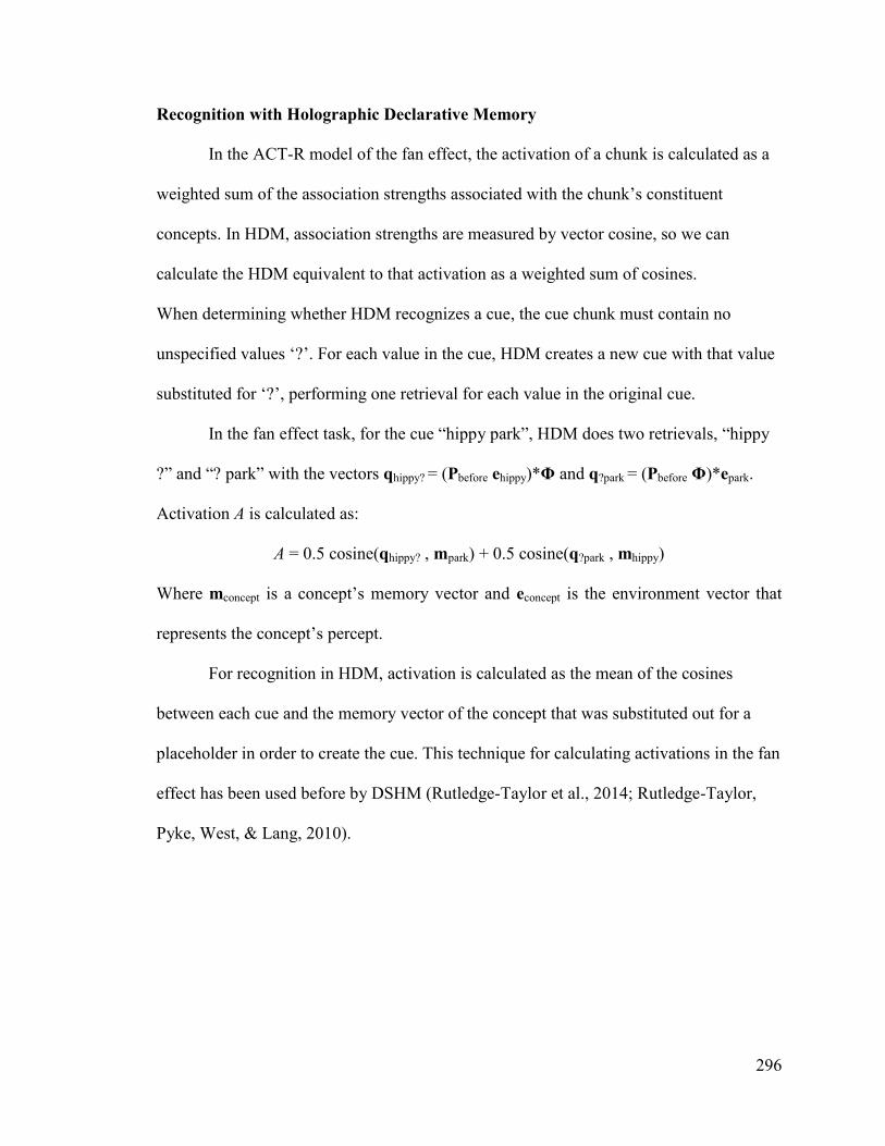
296

Recognition with Holographic Declarative Memory

In the ACT-R model of the fan effect, the activation of a chunk is calculated as a

weighted sum of the association strengths associated with the chunk‟s constituent

concepts. In HDM, association strengths are measured by vector cosine, so we can

calculate the HDM equivalent to that activation as a weighted sum of cosines.

When determining whether HDM recognizes a cue, the cue chunk must contain no

unspecified values „?‟. For each value in the cue, HDM creates a new cue with that value

substituted for „?‟, performing one retrieval for each value in the original cue.

In the fan effect task, for the cue “hippy park”, HDM does two retrievals, “hippy

?” and “? park” with the vectors qhippy? = (Pbefore ehippy)*Φ and q?park = (Pbefore Φ)*epark.

Activation A is calculated as:

A = 0.5 cosine(qhippy? , mpark) + 0.5 cosine(q?park , mhippy)

Where mconcept is a concept’s memory vector and econcept is the environment vector that

represents the concept’s percept.

For recognition in HDM, activation is calculated as the mean of the cosines

between each cue and the memory vector of the concept that was substituted out for a

placeholder in order to create the cue. This technique for calculating activations in the fan

effect has been used before by DSHM (Rutledge-Taylor et al., 2014; Rutledge-Taylor,

Pyke, West, & Lang, 2010).

297

Appendix H Python ACT-R HDM model code for Experiments 1, 2 and 4

This appendix contains the HDM simulation codes for Experiments 1, 2 and 4.

These models are specified in terms of Python ACT-R HDM syntax. The execution of

these models requires the ccm module for Python ACT-R, the HDM module for HDM

and the CFlib module for the complex fan functions.

# Fan effect HDM Simulation for exp 1,2,4

# Author: Kam Kwok, 2015

# Combined Hrq and Hrs models

# Input files: exp_data.txt: 'item1 item2...', e.g.'object color', exp_probes.txt: e.g.'obj is

color'

# FanModel class defines Production rules, memory module used

# lib: CFlib, ccm, time, other libs

# output format: exp record format (csv): probe,ans,rt,f1,f2,date,mem mod; output: a .csv

file

''' FanTest 1) provides a UI, 2) creates the model(FanModel) as a child process, 3) env-to-

model commn: set run conditions,

provides child process commands to signal task done. FanModel is the fan act-r model.

'''

import ccm

from ccm.lib.actr import *

import CFlib

import time

from ccm.lib.actr.hdm import *

#****************

# Utilities

#****************

datafile= ""

probefile = ""

csvfile=""

ansO = None

ansL = None

ans=None

probes=[]

wd={}

fd=()

# I = 845 + p

I = 895

# the experiment

class FanTest(ccm.Model):

def start(self):

global fd,cont,probes,probefile,datafile,ans,ansO,ansL # fan-dictionary, container

298

# Experiment records

exprecs=[]

modelist=[]

trials=0

xlist=[]

rtlist=[]

targets=CFlib.openf2l(datafile)

if app.logf.get():

csvfile = app.e2.get().split(".")[0]+"_results.csv"

hdr=['probe','ans','type','error','RT','fan1','fan2','Total fan','product of

fans','predicted RT','date','mod']

self.fwl2csv(hdr,csvfile)

for item in probes:

frmt_rec=[]

value=None #Total RT

# run agent for each cue

for style in ['byobj','bycolor']:

t1=self.now()

# visual perception time:

yield 0.47

self.style=style

self.obj,self.color=item.split()[0],item.split()[2]

yield self.sayYes,self.sayNo

self.style=None

self.obj=None

self.color=None

## # motor time

## yield 0.21

# motor time for I = 845

yield 0.31

rt=self.now()-t1

if value is None: value=rt

else: value=(value+rt)/2

if style == 'byobj':

ansO = ans

## print "obj ",ans

else:

ansL = ans

## print "loc ",ans

ans = (ansO or ansL)

trials=trials+1

self.obj=None

self.color=None

try:

299

# fan1

fan1 = str(wd[item.split()[0]])

except:

fan1 = '1'

# fan3

try:

fan3 = str(wd[item.split()[2]])

except:

fan3='1'

# process type and ans

s_item = item.split()[0]+' '+item.split()[2]

if s_item in targets:

typ=1

if ans:

error=0

else:

error=1

else:

typ=0

if ans:

error=1

else:

error=0

# log answers

if app.logstatus.get():

log.CFRT_DM[item,str(value),ans]=value

# each trial: for no error

## if ans:

# for plotting

xlist.append(fan1+fan3)

rtlist.append(value)

# exp record format (csv): probe,rt,fo,fc,fl,date,probe#

# exprecs is a list of list

# probe

frmt_rec.append(item)

frmt_rec.append(ans)

frmt_rec.append(typ)

frmt_rec.append(error)

# RT, fan1, container,fan2, fan3

frmt_rec.append(value*1000)

try:

# fan1

f1=wd[item.split()[0]]

except:

300

f1='1'

frmt_rec.append(f1)

## # fan2

## try:

## frmt_rec.append(cont)

## frmt_rec.append(wd[cont])

## except:

## frmt_rec.append('1')

# fan3

try:

# fan3

f3=wd[item.split()[2]]

except:

f3='1'

frmt_rec.append(f3)

tf = int(f1)+int(f3)

frmt_rec.append(tf)

# product of fans

pf = int(f1)* int(f3)

frmt_rec.append(pf)

#prediction: I + rt , I= 845 + p

pRT=CFlib.calrt([item.split()[0],item.split()[2]],datafile)[1]+ I

frmt_rec.append(pRT)

# date

frmt_rec.append(time.ctime())

# id

frmt_rec.append(datafile)

exprecs.append(frmt_rec)

if app.logf.get():

self.fwl2csv(frmt_rec,csvfile)

#plotxy(x_in,y_in,sym = 'ro', xl='Total Fan',

if app.plot.get():

CFlib.plotxy(xlist,rtlist)

def sayYes(self):

global yescount, ans

yescount = yescount+ 1

ans=1

def sayNo(self):

global nocount, ans

nocount = nocount+ 1

ans=0

# for cf container

def sayCont(self,c):

301

global cont

cont = c

# 1)write a list to a csv file

def fwl2csv(self,ilist,ofn):

''' input: ilist = [1,2,a,b] and out-file name, output: a csv file'''

wf = open (ofn,'a')

for item in ilist:

if isinstance(item,str):

wf.write(item+',')

else:

wf.write(str(item)+',')

wf.write('\n')

wf.close()

# 2)write a list of lists to a csv file using fwl2csv

def fwll2csv(self,ilist,ofn):

for item in ilist:

self.fwl2csv(item,ofn)

# used by: App.run_exp

def run_trial():

#root.update()

global nocount, yescount, cont, probes, wd, fd, datafile, probefile

print 'No. of subjects: ',app.s_n.get()

fd={}

wd={}

datafile = app.e1.get()

## print "running trial, ...datafile: ",datafile

probefile = app.e2.get()

try:

probes =[l.strip() for l in open(probefile,'r').readlines()]

except:

print 'No probe file!',probefile

wd = CFlib.f2wd(datafile)

#fd is the fan dictionary: 'obj is loc':[fo,fc,fl]

for line in open(datafile,'r').readlines():

fd =CFlib.line2fdict(line.strip(),wd)

for t in range(1, app.s_n.get()+1):

nocount, yescount=0.0,0.0

env=FanTest()

if app.hdmv.get():

env.model=HrsModel()

else:

env.model=HrqModel()

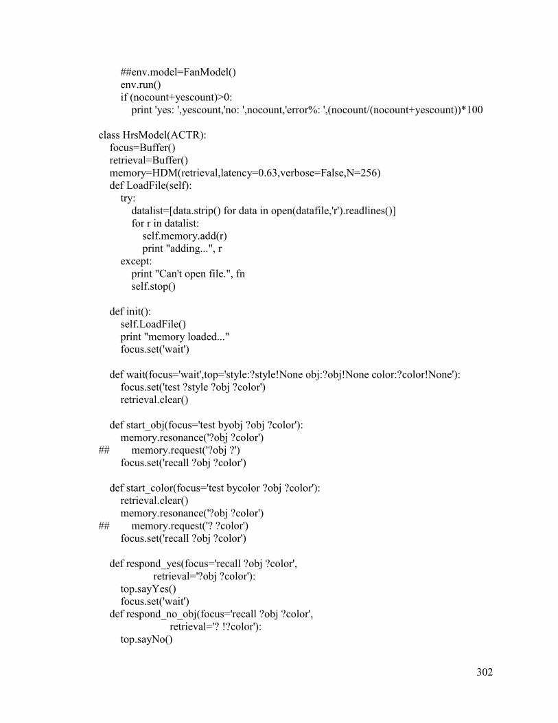
302

##env.model=FanModel()

env.run()

if (nocount+yescount)>0:

print 'yes: ',yescount,'no: ',nocount,'error%: ',(nocount/(nocount+yescount))*100

class HrsModel(ACTR):

focus=Buffer()

retrieval=Buffer()

memory=HDM(retrieval,latency=0.63,verbose=False,N=256)

def LoadFile(self):

try:

datalist=[data.strip() for data in open(datafile,'r').readlines()]

for r in datalist:

self.memory.add(r)

print "adding...", r

except:

print "Can't open file.", fn

self.stop()

def init():

self.LoadFile()

print "memory loaded..."

focus.set('wait')

def wait(focus='wait',top='style:?style!None obj:?obj!None color:?color!None'):

focus.set('test ?style ?obj ?color')

retrieval.clear()

def start_obj(focus='test byobj ?obj ?color'):

memory.resonance('?obj ?color')

## memory.request('?obj ?')

focus.set('recall ?obj ?color')

def start_color(focus='test bycolor ?obj ?color'):

retrieval.clear()

memory.resonance('?obj ?color')

## memory.request('? ?color')

focus.set('recall ?obj ?color')

def respond_yes(focus='recall ?obj ?color',

retrieval='?obj ?color'):

top.sayYes()

focus.set('wait')

def respond_no_obj(focus='recall ?obj ?color',

retrieval='? !?color'):

top.sayNo()

303

retrieval.clear()

focus.set('wait')

def respond_no_color(focus='recall ?obj ?color',

retrieval='!?obj ?'):

top.sayNo()

retrieval.clear()

focus.set('wait')

def respond_no_memerror(focus='recall ?obj ?color',

memory='error:True'):

top.sayNo()

retrieval.clear()

focus.set('wait')

class HrqModel(ACTR):

focus=Buffer()

retrieval=Buffer()

memory=HDM(retrieval,latency=0.63,verbose=False,N=256)

def LoadFile(self):

try:

datalist=[data.strip() for data in open(datafile,'r').readlines()]

for r in datalist:

self.memory.add(r)

print "adding...", r

except:

print "Can't open file.", fn

self.stop()

def init():

self.LoadFile()

print "memory loaded..."

focus.set('wait')

def wait(focus='wait',top='style:?style!None obj:?obj!None color:?color!None'):

focus.set('test ?style ?obj ?color')

retrieval.clear()

def start_obj(focus='test byobj ?obj ?color'):

## memory.resonance('?obj ?color')

memory.request('?obj ?')

focus.set('recall ?obj ?color')

def start_color(focus='test bycolor ?obj ?color'):

retrieval.clear()

## memory.resonance('?obj ?color')

memory.request('? ?color')

focus.set('recall ?obj ?color')

304

def respond_yes(focus='recall ?obj ?color',

retrieval='?obj ?color'):

top.sayYes()

focus.set('wait')

def respond_no_obj(focus='recall ?obj ?color',

retrieval='? !?color'):

top.sayNo()

retrieval.clear()

focus.set('wait')

def respond_no_color(focus='recall ?obj ?color',

retrieval='!?obj ?'):

top.sayNo()

retrieval.clear()

focus.set('wait')

def respond_no_memerror(focus='recall ?obj ?color',

memory='error:True'):

top.sayNo()

retrieval.clear()

focus.set('wait')

#GUI and Main

from Tkinter import *

class App:

def __init__(self, master):

frame = Frame(master)

frame.pack()

self.hdmlog = IntVar(value = 0)

self.hdm = Checkbutton(frame, text = "Verbose mode", variable=self.hdmlog)

self.hdm.pack(side=RIGHT)

self.plot = IntVar(value = 0)

self.opt_plot = Checkbutton(frame, text = "Plot RTs", variable=self.plot)

self.opt_plot.pack(side=RIGHT)

self.logf = IntVar(value = 0)

self.opt_logf = Checkbutton(frame, text = "Save csv file", variable=self.logf)

self.opt_logf.pack(side=RIGHT)

self.logstatus = IntVar(value = 1)

self.opt_logstatus = Checkbutton(frame, text = "Log trials", variable=self.logstatus)

self.opt_logstatus.pack(side=RIGHT)

self.hdmv = IntVar(value = 0)

self.hdm = Checkbutton(frame, text = "HDM Resonance", variable=self.hdmv)

self.hdm.pack(side=RIGHT)

self.s_n = IntVar(value = 1)

self.ss_n = Scale(frame, label = 'No. of subjects:', variable=self.s_n,

from_=1, to=50, tickinterval=24, orient='horizontal')

305

self.ss_n.pack(side=RIGHT)

self.b_run = Button(frame, text="Run Experiment",

fg='red',command=self.run_exp)

self.b_run.pack(side=LEFT)

self.l1 = Label(text="data file:")

self.l1.pack( side = LEFT)

self.dataf = StringVar()

self.dataf.set("exp2_targets.txt")

self.e1 = Entry(bd =5,textvariable=self.dataf)

self.e1.pack(side = LEFT)

self.l2 = Label(text="probes file:")

self.l2.pack( side = LEFT)

self.probef = StringVar()

self.probef.set("exp2_probes.txt")

self.e2 = Entry(bd =5,textvariable=self.probef)

self.e2.pack(side = LEFT)

# This is a handler for the run button - running the experiment

def run_exp(self):

run_trial()

# experiment init

ans=True

log=ccm.log()

root = Tk(className=" Fan Fffect HDM Simulation")

app = App(root)

root.mainloop()

306

Bibliography and References

Ajjanagadde, V., & Shastri, L. (1990). From simple association to systematic reasoning.

Philadelphia, PA: Tech. Report MS-CIS-90-05, University of Pennsylvania.

Anderson, J. R. (1974). Retrieval of propositional information from long-term memory.

Cognitive Psychology 6, no. 4, 451-474.

Anderson, J. R. (1983a). The architecture of cognition. Cambridge, MA: Harvard

University Press.

Anderson, J. R. (1983b). A spreading activation theory of memory. Journal of Verbal

Learning and Verbal Behavior, Vol. 22, 261-295.

Anderson, J. R. (1983b). A spreading activation theory of memory. Journal of Verbal

Learning and Verbal Behavior, Vol. 22, 261-295.

Anderson, J. R. (1991). The place of cognitive architectures in a rational analysis. In K.

Van Len (Ed.), Architectures for Intelligence. Hillsdale, NJ : Erlbaum.

Anderson, J. R. (1995). Cognitive psychology and its implications (4th ed.). New York:

W. H. Freeman.

Anderson, J. R. (2007). How can the human mind occur in the physical universe.

Anderson, J. R., & Bower, G. H. (1980). Human associative memory: revised edition.

Hillsdale, NJ: Erlbaum Associates.

Anderson, J. R., & Lebiere, C. (1998). The Atomic Components of Thought. Mahwah, NJ:

Lawrence Erlbaum.

Anderson, J. R., & Reder, L. M. (1999). The fan effect: New results and new theories.

Journal of Experimental Psychology: General, 128(2), 186–197.

doi:10.1037//0096-3445.128.2.186.

307

Anderson, J. R., & Schooler, L. J. (1991). Reflections of the environment in memory.

Psychological science 2, no. 6, 396-408.

Anderson, J. R., Bothell, D., Byrne, M. D., Douglass, S., Lebiere, C., & Qin, Y. (2004).

An integrated theory of the mind. Psychological Review 111 (4), 1036–60.

doi:10.1037/0033-295X.111.4.1036.

Anderson, J. R., Bothell, D., Lebiere, C., & Matessa, M. (1998). An Integrated Theory of

List Memory. Journal of Memory and Language, 38(4), 341–380.

doi:10.1006/jmla.1997.2553.

Anderson, R. B. (2001). The power law as an emergent property. Memory & cognition,

29(7), 1061-1068.

Anderson, R. B., & Tweney, R. D. (1997). Artifactual power curves in forgetting.

Memory & Cognition, 25(5), 724-730.

Atkinson, R. C., & Shiffrin, R. M. (1968). Human memory: A proposed system and its

control processes. The psychology of learning and motivation, 2, 89-195.

Axtell, R., Axelrod, R., Epstein, J. M., & Cohen, M. D. (1996). Aligning simulation

models: A case study and results. Computational & Mathematical Organization

Theory, 1(2), 123-141.

Balota, D. A., & Lorch, R. F. (1986). Depth of automatic spreading activation: Mediated

priming effects in pronunciation but not in lexical decision. Journal of

Experimental Psychology: Learning, Memory, Cognition Vol. 12, 336-345.

Banks, A. P. (2013). The influence of activation level on belief bias in relational

reasoning. Cognitive science, 37(3), 544-577.

308

Bara, B. G., Bucciarelli, M., & Lombardo, V. (2001). Model theory of deduction: A

unified computational approach. Cognitive Science, 25(6), 839-901.

Barrouillet, P., Plancher, G., Guida, A., & Camos, V. (2013). Forgetting at short term:

When do event-based interference and temporal factors have an effect? Acta

psychologica, 142(2), 155-167.

Bechtel, W., & Graham, G. (1998). A companion to cognitive science. Oxford:

Blackwell.

Bliss, T. V., & Collingridge, G. L. (1993). A synaptic model of memory: long-term

potentiation in the hippocampus. Nature, pp. 31-39.

Bower, G. H. (2000). The Oxford handbook of memory: a brief history of memory

research. The Oxford Press.

Bunting, M. F., Conway, A. R., & Heitz, R. P. (2004). Individual differences in the fan

effect and working memory capacity. Journal of memory and language, 51(4),

604-622.

Cantor, J., & Engle, R. W. (1993). Working memory capacity as long-term memory

activation: An individual-differences approach. Journal of Experimental

Psychology: Learning, Memory, and Cognition, 19, 1101–1114.

Chong, R. S. (2004). Architectural explorations formodeling procedural skill decay.

Proceedings of the Sixth International Conference on Cognitive Modeling.

Mahwah,NJ: Erlbaum.

Collins, A. M., & Loftus, E. F. (1975). A spreading-activation theory of semantic

processing. Psychological Review, 82, 407-428.

309

D'arcy, R. C., Ryner, L., Richter, W., & Connolly, J. F. (2004). The fan effect in fMRI:

Left hemisphere specialization in verbal working memory. Neuroreport, 15(12),

1851-1855.

Donkin, C., & Nosofsky, R. M. (2012). A power-law model of psychological memory

strength in short-and long-term recognition. Psychological Science, 23(6), 625-

634.

Donkin, C., & Nosofsky, R. M. (2012). The structure of short-term memory scanning: An

investigation using response time distribution models. Psychonomic bulletin &

review, 19(3), 363-394.

Dosher, B. A. (1976). The retrieval of sentences from memory: A speed–accuracy study.

Cognitive Psychology, 8, 291–310.

Ebbinghaus, H. (. (1913). Memory (Original work published 1885). New York: Columbia

University, Teachers College.

Eliasmith, C. (2013). How to build a brain: A neural architecture for biological

cognition. Oxford University Press.

Eliasmith, C., & Thagard, P. (2001). Integrating structure and meaning: a distributed

model of analogical mapping. Cognitive Science, pp. 25,245-286.

Franklin, D. R., & Mewhort, D. J. (2013). Control Processes in Free Recall. Franklin, D.

R. J., & Mewhort, D. J. K. (2013). Control Processes in FreProceedings of the

12th International Conference on Cognitive Modeling (pp. pp. 47-52). Ottawa:

Carleton University.

Friston, K. (2003). Learning and inference in the brain. Neural Networks, 16(9), 1325-

1352., 16(9), 1325-1352.

310

Gobet, F., Lane, P. C., Croker, S., Cheng, P. C., Jones, G., Oliver, I., et al. (2001).

Chunking mechanisms in human learning. Trends in cognitive sciences, 5(6), 236-

243.

Goldstein, E. B. (2008). Cognitive Psychology Connecting Mind, Research and Everyday

Experience. Thomson Wadsworth.

Gómez-Ariza, C., & Bajo, M. T. (2003). Interference and integration: The fan effect in

children and adults. Memory, 11(6), 505-523.

Graesser, A. C., Singer, M., & Trabasso, T. (1994). Constructing inferences during

narrative text comprehension. Psychological review, 101(3), 371.

Healy, A., & McNamara, D. (1996). Verbal learning and memory: Does the modal model

still work? Annual Review of Psychology, 47, 143-172. Annual Review of

Psychology, 47, 143-172.

Howell, K. E. (2013). Introduction to the Philosophy of Methodology. London: Sage

Publications.

Jamieson, R. K., & Mewhort, D. J. (2011). Grammaticality is inferred from global

similarity: A reply to Kinder. The Quarterly Journal of Experimental Psychology,

64,, 209-216.

Johnson-Laird, P. N. (1983). Mental models. Cambridge, U.K.: Cambridge University

Press.

Johnson-Laird, P. N., & Byrne, R. (1991). Deduction. Hillsdale, NJ: Lawrence Erlbaum

Associates.

Jones, M. N., & Mewhort, D. J. (2007). Representing word meaning and order

information in a composite holographic lexicon. Psychological Review, 114, 1-37.

311

Kelly, M. A., Mewhort, D. J., & West, R. L. (2014). The memory tesseract: Distributed

MINERVA and the unification of memory. Proceedings of the 36th Annual

Conference of the Cognitive Science Society (pp. 2483-2488). Austin TX:

Cognitive Science Society.

Kelly, M., Kwok, K., & West, R. L. (2015). Holographic Declarative Memory and the

Fan Effect: A Test Case for A New Memory Module for ACT-R. Proceedings of

the 15th International Conference on Cognitive Modeling, (pp. 148-153). Ottawa:

Carleton University.

Kim, J. W., & Ritter, F. E. (2015). Learning, forgetting, and relearning for keystroke-and

mouse-driven tasks: Relearning is important. Human–Computer Interaction,

30(1), 1-33.

Kwok, K., & West, R. L. (2013). SAME: An ACT-R Spreading Activation Modeling

Environment. ICCM-Conference (pp. 366-367). Ottawa: http://iccm-

conference.org/2013-proceedings/papers/0065/paper0065.pdf.

Kwok, K., West, R. L., & Kelly, M. (2015). The fan effect in overlapping data sets and

logical inference. 13th Cognitive Science. Ottawa.

Laird, J. E., Newel, A., & Rosenbloom, P. S. (1987). Soar: An architecture for general

intelligence. Artificial intelligence 33, no. 1, 1-64.

Lewis, C. H., & Anderson, J. R. (1976). Interference with real world knowledge.

Cognitive Psychology, 8(3), 311-335.

Longuet-Higgins, H. C. (1968). Holographic Model of Temporal Recall. Nature, 217,

104.

312

Matthew F. Rutledge-Taylor, A. A. (2010). Modeling a Three Term Fan Effect. 10th

International Conference on Cognitive Modeling, (pp. 211-216). Philadelphia, PA

: Drexel University.

McKoon, G., & Ratcliff, R. (1992). Inference during reading. Psychological review,

99(3), 440.

McNamara, T. P., & V.A., D. (1996). The context of memory retrieval. Journal of

Memory and Language, vol. 35, 877-892.

Melton, A. W. (1963, 2). Implications of short-term memory for a general theory of

memory. Journal of Verbal Learning and Verbal Behavior, pp. 1-21.

Miller, G. A. (1956). The magical number seven, plus or minus two: some limits on our

capacity for processing information. Psychological review, 63(2), 81.

Miller, G. A. (1956). The magical number seven, plus or minus two: some limits on our

capacity for processing information. Psychological review, 63(2), 81-97.

Moeser, S. D. (1979). Moeser, S. D. (1979). The role of experimental design in

investigations of the fan effect. Journal of Experimental Psychology: Human

Learning and Memory, 5(2), 125.

Myers, J. L., O'Brien, E. J., Balota, D. A., & Toyofuku, M. L. (1984). Memory search

without interference: The role of integration. Cognitive Psychology, 16(2), 217-

242.

Newell, A. (1973). You can't play 20 questions with nature and win: Projective

comments on the papers of this symposium.

Newell, A. (1980). Physical Symbol Systems*. Cognitive science, 4(2), 135-183.

Newell, A. (1994). Unified theories of cognition. Harvard University Press.

313

Oberauer, K., & Lewandowsky, S. (2014). Further evidence against decay in working

memory. Journal of Memory and Language, 73, 15-30.

Pachella, R. G. (1974). The interpretation of reaction time in information-processing

research (p 41-82). Hillsdale, NJ: Erlbaum.

Pearson, B., Raškevičius, J., Bays, P. M., Pertzov, Y., & Husain, M. (2014). Working

memory retrieval as a decision process. Journal of vision, 14(2), 2.

Peterson, S. B., & Potts, G. R. (1982). Global and specific components of information

integration. Journal of Verbal Learning and Verbal Behavior, 21(4), 403-420.

Pirolli, P. L., & Anderson, J. R. (1985). The role of practice in fact retrieval. Journal of

experimental psychology: Learning, memory, and cognition, 11(1), 136.

Plate, T. A. (1995, Plate, T. A. (1995). Holographic reduced representations. IEEE

Transactions on Neural Networks, 6, Plate, T. A. (1995). Holographic reduced

representations. IEEE Transactions on Neural Networks, 6, ). Holographic

reduced representations. IEEE Transactions on Neural Networks, 6, 623–641.

Plate, T. A. (2000). Analogy retrieval and processing with distributed vector

representations. Expert Systems: The International Journal of Knowledge

Engineering and Neural Networks, 17, 29-40.

Portrat, S., Barrouillet, P., & Camos, V. (2008). Time-related decay or interference-based

forgetting in working memory? Journal of experimental psychology: Learning,

memory, and cognition, 34(6), 1561.

Radvansky, G. A. (1999). The fan effect: A tale of two theories. Journal of Experimental

Psychology: General, 128(2), 198-206.

314

Radvansky, G. A., & Zacks, R. T. (1991). Mental models and the fan effect. Journal of

Experimental Psychology: Learning, Memory, and Cognition, 17(5), 940-953.

Radvansky, G. A., Spieler, D. H., & Zacks, R. T. (1993). Mental model organization.

Journal of Experimental Psychology 19(1), 95-114.

Rahman, A. K. (1967). Decay and interference in short-term recognition memory. Thesis.

Montreal, Quebec, Order No. NK02230, McGill University (Canada)). ProQuest

Dissertations and Theses, , 0-1. Retrieved from

http://search.proquest.com/docview/302287880?accountid=9894. (302287880).:

McGill University.

Ratcliff, R. (1978). A theory of memory retrieval. Psychological review, 85(2), 59.

Reder, L. M., & Anderson, J. R. (1980). A partial resolution of the paradox of

interference: The role of integrating knowledge. Cognitive Psychology, 12(4),

447-472.

Reder, L. M., & Anderson, J. R. (1980.). A partial resolution of the paradox of

interference: The role of integrating knowledge. Cognitive Psychology, 12(4),

447-472.

Reder, L. M., & Ross, B. H. (1983). Integrated knowledge in different tasks: The role of

retrieval strategy on fan effects. Journal of Experimental Psychology: Learning,

Memory, and Cognition, 9(1), 55.

Ricks, T. R., & Wiley, J. (2010). Do Baseball Fans Experience the Fan Effect?.

Proceedings of the Annual Conference of the Cognitive Science Society.

Roberts, S., & Pashler, H. (2000). How persuasive is a good fit? A comment on theory

testing. Psychological review, 107(2),358.

315

Roberts, S., & Pashler, H. (2002). Reply to Rodgers and Rowe.

Roediger, H. L., Knight, J. L., & Kantowitz, B. H. (1977). Inferring decay in short-term

memory: The issue of capacity. Memory & cognition, 5(2), 167-176.

Rosenbloom, P. S., Laird, J. E., & Newell, A. E. (1993). The Soar papers: Research on

integrated intelligence , Vols. 1 & 2. MIT Press.

Rutledge-Taylor, M. (2005). Can ACT-R realize” Newell‟s dream”. Proceedings of the

27th annual meeting of the Cognitive Science Society. Indiana: University of

Indiana.

Rutledge-Taylor, M. F. (2014). Dynamically structured holographic memory.

Biologically Inspired Cognitive Architectures, 9, 9-32.

Rutledge-Taylor, M. F., & West, R. L. (2011). Using DSHM to model paper, rock,

scissors. Proceedings of the 33rd Annual Conference of the Cognitive Science

Society, (pp. pp. 2341-2346).

Rutledge-Taylor, M. F., Kelly, M. A., West, R. L., & Pyke, A. A. (2014). Dynamically

structured holographic memory. Biologically Inspired Cognitive Architectures, 9,

9-32.

Rutledge-Taylor, M. F., Pyke, A. A., West, R. L., & Lang, H. (2010). Modeling a three

term fan effect. Proceedings of the 10th International Conference on Cognitive

Modeling (pp. pp. 211-216). Philadelphia, PA: Drexel University.

Rutledge-Taylor, M. F., Vellino, A., & West, R. L. (2008). A holographic associative

memory recommender system. the 3rd International Conference on Digital

Information Management, (pp. pp. 87-92). London, UK.

316

Samsonovich, A. V. (2010). Toward a Unified Catalog of Implemented Cognitive

Architectures. Biologically Inspired Cognitive Architecture (BICA) 221, 195-244.

Schneider, D. W., & Anderson, J. R. (2011). A memory-based model of Hick‟s law.

Cognitive Psychology, 193-222.

Schneider, D. W., & Anderson, J. R. (2012). Modeling fan effects on the time course of

associative recognition. Cognitive psychology, 64(3), 127-160.

Schultheis, H., Lile, S., & Barkowsky, T. (2007). Extending act-r‟s memory capabilities.

Proceedings of EuroCogSci, (pp. 7, 758-763.).

Sejnowski, T. J., & Tesauro, G. (1989). The Hebb rule for synaptic plasticity: algorithms

and implementations. In J. H. (ed.), Neural models of plasticity: Experimental and

theoretical approaches (pp. 94-103).

Sejnowski, T. J., & Tesauro, G. (1989). The Hebb rule for synaptic plasticity: algorithms

and implementations. In J. H. (ed.), Neural models of plasticity: Experimental and

theoretical approaches (pp. 94-103).

Sharifian, F., & R., S. (1997). Hierarchical spreading of activation. Proceedings of the

Conference on Language, Cognition, and Interpretation; F. Sharifian (Ed.) (pp.

1-10). Isfahan: IAU Press.

Shepard, R. N. (1984). Ecological constraints on internal representation: Resonant

kinematics of perceiving, imagining, thinking, and dreaming. Psychological

Review, 91(4), 417-447.

Simon, H. A., & Wallach, D. (1999). Cognitive modeling in perspective.

Kognitionswissenschaft, 8(1), 1-4.

317

Sohn, M.-H., Anderson, J. R., Reder, L. M., & Goode, A. (2004). Differential fan effect

and attentional focus. Differential Psychonomic Bulletin & Review, 11(4), 729–

34. Retrieved from http://www.ncbi.nlm.nih.gov/pubmed/15581125.

Staddon, J. E. (1988). Learning as inference. Evolution and learning. books.google.com.

Sternberg, S. (1966). High-speed scanning in human memory. Science, 153(3736), 652-

654.

Sternberg, S. (1969). The discovery of processing stages: Extensions of Donders' method.

Acta psychologica, 30, 276-315.

Stevens, S. S. (1957). On the psychophysical law. Psychological review, 64(3), 153.

Stewart, T. C., & Eliasmith, C. (2009). Spiking neurons and central executive control:

The origin of the 50-millisecond cognitive cycle. 9th International Conference on

Cognitive Modelling, (pp. 122-127). Manchester: University of Manchester.

Stewart, T. C., & West, R. L. (2006). Deconstructing ACT-R. Seventh International

Conference on Cognitive Modeling, (pp. 298-303). Ottawa.

Stewart, T. C., & West, R. L. (2010). Testing for equivalence: a methodology for

computational cognitive modelling. Journal of Artificial General Intelligence 2.2,

69-87.

Sun, R. (2002). Duality of the Mind: A Bottom-up Approach Toward Cognition. Mahwah

NJ: Lawrence Erlbaum Associates.

Sun, R. (2006). The CLARION cognitive architecture: Extending cognitive modeling to

social simulation. In The CLARION cognitive architecture: Extending cognitive

modeling to social simulation (pp. 79-99).

318

Sun, R. (2008). The Cambridge handbook of computational psychology. Cambridge

University Press.

Tulving, E. &. (1992). On the nature of the Tulving-Wiseman function.

West, R. L., Pyke, A. A., Rutledge-Taylor, M. F., & Lang, H. (2010). Interference and

ACT-R: New evidence from the fan effect. 10th International Conference on

Cognitive Modeling, (pp. 211-216). Philadelphia, PA: Drexel University.

Wickelgren, W. A. (1977). Speed–accuracy tradeoff and information processing

dynamics. Acta Psychologica, 41, 67–85.

Wixted, J. T., & Carpenter, S. K. (2007). The Wickelgren power law and the Ebbinghaus

savings function. Psychological Science, 18(2), 133-134.