Complex Analysis

George Cain

(c)Copyright 1999 by George Cain. All rights reserved.

Table of Contents

Chapter One - Complex Numbers 1.1 Introduction 1.2 Geometry 1.3 Polar coordinates

Chapter Two - Complex Functions 2.1 Functions of a real variable 2.2 Functions of a complex variable 2.3 Derivatives

Chapter Three - Elementary Functions 3.1 Introduction 3.2 The exponential function 3.3 Trigonometric functions 3.4 Logarithms and complex exponents

Chapter Four - Integration 4.1 Introduction 4.2 Evaluating integrals 4.3 Antiderivatives

Chapter Five - Cauchy's Theorem 5.1 Homotopy 5.2 Cauchy's Theorem

Chapter Six - More Integration 6.1 Cauchy's Integral Formula 6.2 Functions defined by integrals 6.3 Liouville's Theorem 6.4 Maximum moduli

Chapter Seven - Harmonic Functions 7.1 The Laplace equation 7.2 Harmonic functions 7.3 Poisson's integral formula

Chapter Eight - Series 8.1 Sequences 8.2 Series 8.3 Power series 8.4 Integration of power series 8.5 Differentiation of power series

Chapter Nine - Taylor and Laurent Series 9.1 Taylor series 9.2 Laurent series

Chapter Ten - Poles, Residues, and All That 10.1 Residues 10.2 Poles and other singularities

Chapter Eleven - Argument Principle 11.1 Argument principle 11.2 Rouche's Theorem

----------------------------------------------------------------------------George CainSchool of MathematicsGeorgia Institute of TechnologyAtlanta, Georgia 0332-0160

cain@math.gatech.edu

Chapter One

Complex Numbers

1.1 Introduction. Let us hark back to the first grade when the only numbers you knewwere the ordinary everyday integers. You had no trouble solving problems in which youwere, for instance, asked to find a number x such that 3x 6. You were quick to answer”2”. Then, in the second grade, Miss Holt asked you to find a number x such that 3x 8.You were stumped—there was no such ”number”! You perhaps explained to Miss Holt that32 6 and 33 9, and since 8 is between 6 and 9, you would somehow need a numberbetween 2 and 3, but there isn’t any such number. Thus were you introduced to ”fractions.”

These fractions, or rational numbers, were defined by Miss Holt to be ordered pairs ofintegers—thus, for instance, 8,3 is a rational number. Two rational numbers n,m andp,q were defined to be equal whenever nq pm. (More precisely, in other words, arational number is an equivalence class of ordered pairs, etc.) Recall that the arithmetic ofthese pairs was then introduced: the sum of n,m and p,q was defined by

n,m p,q nq pm,mq,

and the product by

n,mp,q np,mq.

Subtraction and division were defined, as usual, simply as the inverses of the twooperations.

In the second grade, you probably felt at first like you had thrown away the familiarintegers and were starting over. But no. You noticed that n, 1 p, 1 n p, 1 andalso n, 1p, 1 np, 1. Thus the set of all rational numbers whose second coordinate isone behave just like the integers. If we simply abbreviate the rational number n, 1 by n,there is absolutely no danger of confusion: 2 3 5 stands for 2,1 3,1 5,1. Theequation 3x 8 that started this all may then be interpreted as shorthand for the equation3,1u,v 8,1, and one easily verifies that x u,v 8,3 is a solution. Now, ifsomeone runs at you in the night and hands you a note with 5 written on it, you do notknow whether this is simply the integer 5 or whether it is shorthand for the rational number5,1. What we see is that it really doesn’t matter. What we have ”really” done isexpanded the collection of integers to the collection of rational numbers. In other words,we can think of the set of all rational numbers as including the integers–they are simply therationals with second coordinate 1.

One last observation about rational numbers. It is, as everyone must know, traditional to

1.1

write the ordered pair n,m as nm . Thus n stands simply for the rational number n

1 , etc.

Now why have we spent this time on something everyone learned in the second grade?Because this is almost a paradigm for what we do in constructing or defining the so-calledcomplex numbers. Watch.

Euclid showed us there is no rational solution to the equation x2 2. We were thus led todefining even more new numbers, the so-called real numbers, which, of course, include therationals. This is hard, and you likely did not see it done in elementary school, but we shallassume you know all about it and move along to the equation x2 1. Now we definecomplex numbers. These are simply ordered pairs x,y of real numbers, just as therationals are ordered pairs of integers. Two complex numbers are equal only when thereare actually the same–that is x,y u,v precisely when x u and y v. We define thesum and product of two complex numbers:

x,y u,v x u,y v

andx,yu,v xu yv,xv yu

As always, subtraction and division are the inverses of these operations.

Now let’s consider the arithmetic of the complex numbers with second coordinate 0:

x, 0 u, 0 x u, 0,

andx, 0u, 0 xu, 0.

Note that what happens is completely analogous to what happens with rationals withsecond coordinate 1. We simply use x as an abbreviation for x, 0 and there is no danger ofconfusion: x u is short-hand for x, 0 u, 0 x u, 0 and xu is short-hand forx, 0u, 0. We see that our new complex numbers include a copy of the real numbers, justas the rational numbers include a copy of the integers.

Next, notice that xu,v u,vx x, 0u,v xu,xv. Now then, any complex numberz x,y may be written

1.2

z x,y x, 0 0,y x y0,1

When we let 0,1, then we have

z x,y x y

Now, suppose z x,y x y and w u,v u v. Then we have

zw x yu v xu xv yu 2yv

We need only see what 2 is: 2 0,10,1 1,0, and we have agreed that we cansafely abbreviate 1,0 as 1. Thus, 2 1, and so

zw xu yv xv yu

and we have reduced the fairly complicated definition of complex arithmetic simply toordinary real arithmetic together with the fact that 2 1.

Let’s take a look at division–the inverse of multiplication. Thus zw stands for that complex

number you must multiply w by in order to get z . An example:

zw x y

u v x yu v

u vu v

xu yv yu xvu2 v2

xu yvu2 v2

yu xvu2 v2

Note this is just fine except when u2 v2 0; that is, when u v 0. We may thus divideby any complex number except 0 0,0.

One final note in all this. Almost everyone in the world except an electrical engineer usesthe letter i to denote the complex number we have called . We shall accordingly use irather than to stand for the number 0,1.

Exercises

1.3

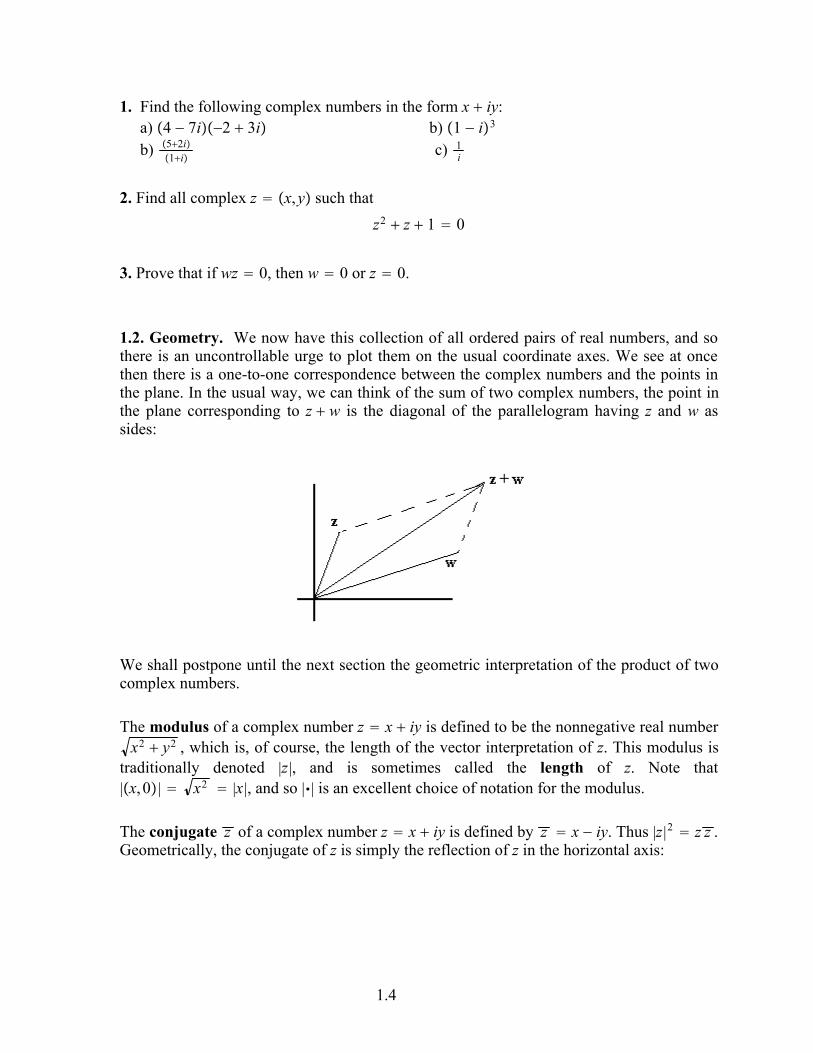
1. Find the following complex numbers in the form x iy:a) 4 7i2 3i b) 1 i3

b) 52i1i c) 1

i

2. Find all complex z x,y such thatz2 z 1 0

3. Prove that if wz 0, then w 0 or z 0.

1.2. Geometry. We now have this collection of all ordered pairs of real numbers, and sothere is an uncontrollable urge to plot them on the usual coordinate axes. We see at oncethen there is a one-to-one correspondence between the complex numbers and the points inthe plane. In the usual way, we can think of the sum of two complex numbers, the point inthe plane corresponding to z w is the diagonal of the parallelogram having z and w assides:

We shall postpone until the next section the geometric interpretation of the product of twocomplex numbers.

The modulus of a complex number z x iy is defined to be the nonnegative real numberx2 y2 , which is, of course, the length of the vector interpretation of z. This modulus istraditionally denoted |z|, and is sometimes called the length of z. Note that|x, 0| x2 |x|, and so || is an excellent choice of notation for the modulus.

The conjugate z of a complex number z x iy is defined by z x iy. Thus |z|2 z z .Geometrically, the conjugate of z is simply the reflection of z in the horizontal axis:

1.4

Observe that if z x iy and w u iv, then

z w x u iy v x iy u iv z w.

In other words, the conjugate of the sum is the sum of the conjugates. It is also true thatzw z w. If z x iy, then x is called the real part of z, and y is called the imaginarypart of z. These are usually denoted Re z and Im z, respectively. Observe then thatz z 2Re z and z z 2Im z.

Now, for any two complex numbers z and w consider

|z w|2 z wz w z w z w z z w z wz ww |z|2 2Rew z |w|2

|z|2 2|z||w| |w|2 |z| |w|2

In other words,

|z w| |z| |w|the so-called triangle inequality. (This inequality is an obvious geometric fact–can youguess why it is called the triangle inequality?)

Exercises

4. a)Prove that for any two complex numbers, zw z w.b)Prove that zw z

w .c)Prove that ||z| |w|| |z w|.

5. Prove that |zw| |z||w| and that | zw | |z||w | .

1.5

6. Sketch the set of points satisfyinga) |z 2 3i| 2 b)|z 2i| 1c) Re z i 4 d) |z 1 2i| |z 3 i|e)|z 1| |z 1| 4 f) |z 1| |z 1| 4

1.3. Polar coordinates. Now let’s look at polar coordinates r, of complex numbers.Then we may write z rcos i sin. In complex analysis, we do not allow r to benegative; thus r is simply the modulus of z. The number is called an argument of z, andthere are, of course, many different possibilities for . Thus a complex numbers has aninfinite number of arguments, any two of which differ by an integral multiple of 2. Weusually write arg z. The principal argument of z is the unique argument that lies onthe interval ,.

Example. For 1 i, we have

1 i 2 cos 74 i sin 7

4

2 cos 4 i sin 4

2 cos 3994 i sin 399

4

etc., etc., etc. Each of the numbers 74 ,

4 , and

3994 is an argument of 1 i, but the

principal argument is 4 .

Suppose z rcos i sin and w scos i sin. Thenzw rcos i sinscos i sin

rscoscos sin sin isincos sincos rscos i sin

We have the nice result that the product of two complex numbers is the complex numberwhose modulus is the product of the moduli of the two factors and an argument is the sumof arguments of the factors. A picture:

1.6

We now define expi, or ei byei cos i sin

We shall see later as the drama of the term unfolds that this very suggestive notation is anexcellent choice. Now, we have in polar form

z rei,

where r |z| and is any argument of z. Observe we have just shown that

eiei ei.

It follows from this that eiei 1. Thus

1ei

ei

It is easy to see that

zw rei

sei rs cos i sin

Exercises

7. Write in polar form rei:a) i b) 1 ic) 2 d) 3ie) 3 3i

8.Write in rectangular form—no decimal approximations, no trig functions:a) 2ei3 b) ei100c) 10ei/6 d) 2 ei5/4

9. a) Find a polar form of 1 i1 i 3 .b) Use the result of a) to find cos 7

12 and sin 712 .

10. Find the rectangular form of 1 i100.

1.7

11. Find all z such that z3 1. (Again, rectangular form, no trig functions.)

12. Find all z such that z4 16i. (Rectangular form, etc.)

1.8

Chapter Two

Complex Functions

2.1. Functions of a real variable. A function : I C from a set I of reals into thecomplex numbers C is actually a familiar concept from elementary calculus. It is simply afunction from a subset of the reals into the plane, what we sometimes call a vector-valuedfunction. Assuming the function is nice, it provides a vector, or parametric, descriptionof a curve. Thus, the set of all t : t eit cos t i sin t cos t, sin t, 0 t 2is the circle of radius one, centered at the origin.

We also already know about the derivatives of such functions. If t xt iyt, thenthe derivative of is simply t x t iy t, interpreted as a vector in the plane, it istangent to the curve described by at the point t.

Example. Let t t it2, 1 t 1. One easily sees that this function describes thatpart of the curve y x2 between x 1 and x 1:

0

1

-1 -0.5 0.5 1x

Another example. Suppose there is a body of mass M ”fixed” at the origin–perhaps thesun–and there is a body of mass m which is free to move–perhaps a planet. Let the locationof this second body at time t be given by the complex-valued function zt. We assume theonly force on this mass is the gravitational force of the fixed body. This force f is thus

f GMm|zt|2

zt|zt|

where G is the universal gravitational constant. Sir Isaac Newton tells us that

mzt f GMm|zt|2

zt|zt|

2.1

Hence,

z GM|z|3

z

Next, let’s write this in polar form, z rei:

d2dt2

rei kr2ei

where we have written GM k. Now, let’s see what we have.

ddt re

i r ddt ei drdt e

i

Now,

ddt e

i ddt cos i sin

sin icos ddt icos i sin ddt i ddt e

i.

(Additional evidence that our notation ei cos i sin is reasonable.)Thus,

ddt re

i r ddt ei drdt e

i

r i ddt ei drdt e

i

drdt ir

ddt ei.

Now,

2.2

d2dt2

rei d2rdt2

i drdtddt ir

d2dt2

ei

drdt ir

ddt i ddt e

i

d2rdt2

r ddt

2 i r d

2dt2

2 drdtddt ei

Now, the equation d2dt2 re

i kr2ei becomes

d2rdt2

r ddt

2 i r d

2dt2

2 drdtddt k

r2.

This gives us the two equations

d2rdt2

r ddt

2 k

r2,

and,

r d2dt2

2 drdtddt 0.

Multiply by r and this second equation becomes

ddt r2 ddt 0.

This tells us that

r2 ddt

is a constant. (This constant is called the angular momentum.) This result allows us toget rid of d

dt in the first of the two differential equations above:

d2rdt2

r r2

2 k

r2

or,

d2rdt2

2r3

kr2.

2.3

Although this now involves only the one unknown function r, as it stands it is tough tosolve. Let’s change variables and think of r as a function of . Let’s also write things interms of the function s 1

r . Then,

ddt

ddt

dd

r2dd .

Hence,drdt

r2drd dsd ,

and sod2rdt2

ddt

dsd s2 dd dsd

2s2 d2sd2

,

and our differential equation looks like

d2rdt2

2r3

2s2 d2sd2

2s3 ks2,

or,d2sd2

s k2.

This one is easy. From high school differential equations class, we remember that

s 1r Acos k

2,

where A and are constants which depend on the initial conditions. At long last,

r 2/k1 cos ,

where we have set A2/k. The graph of this equation is, of course, a conic section ofeccentricity .

Exercises

2.4

1. a)What curve is described by the function t 3t 4 it 6, 0 t 1 ?b)Suppose z and w are complex numbers. What is the curve described by

t 1 tw tz, 0 t 1 ?

2. Find a function that describes that part of the curve y 4x3 1 between x 0 andx 10.

3. Find a function that describes the circle of radius 2 centered at z 3 2i .

4. Note that in the discussion of the motion of a body in a central gravitational force field,it was assumed that the angular momentum is nonzero. Explain what happens in case 0.

2.2 Functions of a complex variable. The real excitement begins when we considerfunction f : D C in which the domain D is a subset of the complex numbers. In somesense, these too are familiar to us from elementary calculus—they are simply functionsfrom a subset of the plane into the plane:

fz fx,y ux,y ivx,y ux,y,vx,y

Thus fz z2 looks like fz z2 x iy2 x2 y2 2xyi. In other words,ux,y x2 y2 and vx,y 2xy. The complex perspective, as we shall see, generallyprovides richer and more profitable insights into these functions.

The definition of the limit of a function f at a point z z0 is essentially the same as thatwhich we learned in elementary calculus:

zz0lim fz L

means that given an 0, there is a so that |fz L| whenever 0 |z z0 | . Asyou could guess, we say that f is continuous at z0 if it is true that

zz0lim fz fz0. If f is

continuous at each point of its domain, we say simply that f is continuous.

Suppose bothzz0lim fz and

zz0lim gz exist. Then the following properties are easy to

establish:

2.5

zz0lim fz gz

zz0lim fz

zz0lim gz

zz0lim fzgz

zz0lim fz

zz0lim gz

and,

zz0lim fz

gz zz0lim fz

zz0lim gz

provided, of course, thatzz0lim gz 0.

It now follows at once from these properties that the sum, difference, product, and quotientof two functions continuous at z0 are also continuous at z0. (We must, as usual, except thedreaded 0 in the denominator.)

It should not be too difficult to convince yourself that if z x,y, z0 x0,y0, andfz ux,y ivx,y, then

zz0lim fz

x,yx0,y0lim ux,y i

x,yx0,y0lim vx,y

Thus f is continuous at z0 x0,y0 precisely when u and v are.

Our next step is the definition of the derivative of a complex function f. It is the obviousthing. Suppose f is a function and z0 is an interior point of the domain of f . The derivativef z0 of f is

f z0 zz0lim fz fz0

z z0

Example

Suppose fz z2 . Then, letting z z z0, we have

2.6

zz0lim fz fz0

z z0 z0lim fz0 z fz0

z

z0lim z0 z2 z02

z

z0lim 2z0z z2

z

z0lim 2z0 z

2z0

No surprise here–the function fz z2 has a derivative at every z, and it’s simply 2z.

Another Example

Let fz zz. Then,

z0lim fz0 z fz0

z z0lim z0 zz0 z z0 z 0

z

z0lim z0z z 0z zz

z

z0lim z 0 z z0 zz

Suppose this limit exists, and choose z x, 0. Then,

z0lim z 0 z z0 zz

x0lim z 0 x z0 xx

z 0 z0Now, choose z 0,y. Then,

z0lim z 0 z z0 zz

y0lim z 0 iy z0 iyiy

z 0 z0

Thus, we must have z 0 z0 z 0 z0, or z0 0. In other words, there is no chance ofthis limit’s existing, except possibly at z0 0. So, this function does not have a derivativeat most places.

Now, take another look at the first of these two examples. It looks exactly like what you

2.7

did in Mrs. Turner’s 3rd grade calculus class for plain old real-valued functions. Meditateon this and you will be convinced that all the ”usual” results for real-valued functions alsohold for these new complex functions: the derivative of a constant is zero, the derivative ofthe sum of two functions is the sum of the derivatives, the ”product” and ”quotient” rulesfor derivatives are valid, the chain rule for the composition of functions holds, etc., etc. Forproofs, you need only go back to your elementary calculus book and change x’s to z’s.

A bit of jargon is in order. If f has a derivative at z0, we say that f is differentiable at z0. Iff is differentiable at every point of a neighborhood of z0, we say that f is analytic at z0. (Aset S is a neighborhood of z0 if there is a disk D z : |z z0 | r, r 0 so that D S.) If f is analytic at every point of some set S, we say that f is analytic on S. A function thatis analytic on the set of all complex numbers is said to be an entire function.

Exercises

5. Suppose fz 3xy ix y2. Findz32ilim fz, or explain carefully why it does not

exist.

6. Prove that if f has a derivative at z, then f is continuous at z.

7. Find all points at which the valued function f defined by fz z has a derivative.

8. Find all points at which the valued function f defined byfz 2 iz3 iz2 4z 1 7i

has a derivative.

9. Is the function f given by

fz z 2z , z 0

0 , z 0

differentiable at z 0? Explain.

2.3. Derivatives. Suppose the function f given by fz ux,y ivx,y has a derivativeat z z0 x0,y0. We know this means there is a number f z0 so that

f z0 z0lim fz0 z fz0

z .

2.8

Choose z x, 0 x. Then,

f z0 z0lim fz0 z fz0

z

x0lim ux0 x,y0 ivx0 x,y0 ux0,y0 ivx0,y0

x

x0lim ux0 x,y0 ux0,y0

x i vx0 x,y0 vx0,y0x

ux x0,y0 i

vx x0,y0

Next, choose z 0,y iy. Then,

f z0 z0lim fz0 z fz0

z

y0lim ux0,y0 y ivx0,y0 y ux0,y0 ivx0,y0

iy

y0lim vx0,y0 y vx0,y0

y i ux0,y0 y ux0,y0y

vy x0,y0 i

uy x0,y0

We have two different expressions for the derivative f z0, and so

ux x0,y0 i

vx x0,y0

vy x0,y0 i

uy x0,y0

or,

ux x0,y0

vy x0,y0,

uy x0,y0

vx x0,y0

These equations are called the Cauchy-Riemann Equations.

We have shown that if f has a derivative at a point z0, then its real and imaginary partssatisfy these equations. Even more exciting is the fact that if the real and imaginary parts off satisfy these equations and if in addition, they have continuous first partial derivatives,then the function f has a derivative. Specifically, suppose ux,y and vx,y have partialderivatives in a neighborhood of z0 x0,y0, suppose these derivatives are continuous atz0, and suppose

2.9

ux x0,y0

vy x0,y0,

uy x0,y0

vx x0,y0.

We shall see that f is differentiable at z0.

fz0 z fz0z

ux0 x,y0 y ux0,y0 ivx0 x,y0 y vx0,y0x iy .

Observe that

ux0 x,y0 y ux0,y0 ux0 x,y0 y ux0,y0 y ux0,y0 y ux0,y0.

Thus,

ux0 x,y0 y ux0,y0 y x ux ,y0 y,

and,ux ,y0 y

ux x0,y0 1,

where,

z0lim 1 0.

Thus,

ux0 x,y0 y ux0,y0 y x ux x0,y0 1 .

Proceeding similarly, we get

2.10

fz0 z fz0z

ux0 x,y0 y ux0,y0 ivx0 x,y0 y vx0,y0x iy

x u

x x0,y0 1 ivx x0,y0 i 2 y u

y x0,y0 3 ivy x0,y0 i 4

x iy , .

where i 0 as z 0. Now, unleash the Cauchy-Riemann equations on this quotient andobtain,

fz0 z fz0z

x u

x ivx iy u

x ivx

x iy stuffx iy

ux i v

x stuffx iy .

Here,stuff x1 i 2 y3 i 4.

It’s easy to show that

z0lim stuff

z 0,

and so,

z0lim fz0 z fz0

z ux i v

x .

In particular we have, as promised, shown that f is differentiable at z0.

Example

Let’s find all points at which the function f given by fz x3 i1 y3 is differentiable.Here we have u x3 and v 1 y3. The Cauchy-Riemann equations thus look like

3x2 31 y2, and0 0.

2.11

The partial derivatives of u and v are nice and continuous everywhere, so f will bedifferentiable everywhere the C-R equations are satisfied. That is, everywhere

x2 1 y2; that is, wherex 1 y, or x 1 y.

This is simply the set of all points on the cross formed by the two straight lines

-2

-1

0

1

2

3

4

-3 -2 -1 1 2 3x

Exercises

10. At what points is the function f given by fz x3 i1 y3 analytic? Explain.

11. Do the real and imaginary parts of the function f in Exercise 9 satisfy theCauchy-Riemann equations at z 0? What do you make of your answer?

12. Find all points at which fz 2y ix is differentiable.

13. Suppose f is analytic on a connected open set D, and f z 0 for all zD. Prove that fis constant.

14. Find all points at which

fz xx2 y2

i yx2 y2

is differentiable. At what points is f analytic? Explain.

15. Suppose f is analytic on the set D, and suppose Re f is constant on D. Is f necessarily

2.12

constant on D? Explain.

16. Suppose f is analytic on the set D, and suppose |fz| is constant on D. Is f necessarilyconstant on D? Explain.

2.13

Chapter Three

Elementary Functions

3.1. Introduction. Complex functions are, of course, quite easy to come by—they aresimply ordered pairs of real-valued functions of two variables. We have, however, alreadyseen enough to realize that it is those complex functions that are differentiable that are themost interesting. It was important in our invention of the complex numbers that these newnumbers in some sense included the old real numbers—in other words, we extended thereals. We shall find it most useful and profitable to do a similar thing with many of thefamiliar real functions. That is, we seek complex functions such that when restricted to thereals are familiar real functions. As we have seen, the extension of polynomials andrational functions to complex functions is easy; we simply change x’s to z’s. Thus, forinstance, the function f defined by

fz z2 z 1z 1

has a derivative at each point of its domain, and for z x 0i, becomes a familiar realrational function

fx x2 x 1x 1 .

What happens with the trigonometric functions, exponentials, logarithms, etc., is not soobvious. Let us begin.

3.2. The exponential function. Let the so-called exponential function exp be defined by

expz excosy i siny,

where, as usual, z x iy. From the Cauchy-Riemann equations, we see at once that thisfunction has a derivative every where—it is an entire function. Moreover,

ddz expz expz.

Note next that if z x iy and w u iv, then

3.1

expz w exucosy v i siny v exeycosycosv siny sinv isinycosv cosy sinv exeycosy i sinycosv i sinv expzexpw.

We thus use the quite reasonable notation ez expz and observe that we have extendedthe real exponential ex to the complex numbers.

Example

Recall from elementary circuit analysis that the relation between the voltage drop V and thecurrent flow I through a resistor is V RI, where R is the resistance. For an inductor, therelation is V L dIdt , where L is the inductance; and for a capacitor, C

dVdt I, where C is

the capacitance. (The variable t is, of course, time.) Note that if V is sinusoidal with afrequency , then so also is I. Suppose then that V A sint . We can write this asV ImAeieit ImBeit, where B is complex. We know the current I will have thissame form: I ImCeit. The relations between the voltage and the current are linear, andso we can consider complex voltages and currents and use the fact thateit cost i sint. We thus assume a more or less fictional complex voltage V , theimaginary part of which is the actual voltage, and then the actual current will be theimaginary part of the resulting complex current.

What makes this a good idea is the fact that differentiation with respect to time t becomessimply multiplication by i: d

dt Aeit iAeit. If I beit, the above relations between

current and voltage become V iLI for an inductor, and iVC I, or V IiC for a

capacitor. Calculus is thereby turned into algebra. To illustrate, suppose we have a simpleRLC circuit with a voltage source V a sint. We let E aeiwt .

Then the fact that the voltage drop around a closed circuit must be zero (one of Kirchoff’scelebrated laws) looks like

3.2

iLI IiC RI aeit, or

iLb biC Rb a

Thus,b a

R i L 1C

.

In polar form,

b aR2 L 1

C2ei,

where

tan L 1

CR . (R 0)

Hence,

I Imbeit Im aR2 L 1

C2eit

aR2 L 1

C2sint

This result is well-known to all, but I hope you are convinced that this algebraic approachafforded us by the use of complex numbers is far easier than solving the differentialequation. You should note that this method yields the steady state solution—the transientsolution is not necessarily sinusoidal.

Exercises

1. Show that expz 2i expz.

2. Show that expzexpw expz w.

3. Show that |expz| ex, and argexpz y 2k for any argexpz and some

3.3

integer k.

4. Find all z such that expz 1, or explain why there are none.

5. Find all z such that expz 1 i, or explain why there are none.

6. For what complex numbers w does the equation expz w have solutions? Explain.

7. Find the indicated mesh currents in the network:

3.3 Trigonometric functions. Define the functions cosine and sine as follows:

cos z eiz eiz2 ,

sin z eiz eiz2i

where we are using ez expz.

First, let’s verify that these are honest-to-goodness extensions of the familiar real functions,cosine and sine–otherwise we have chosen very bad names for these complex functions.So, suppose z x 0i x. Then,

eix cosx i sinx, andeix cosx i sinx.

Thus,

3.4

cosx eix eix2 ,

sinx eix eix2i ,

and everything is just fine.

Next, observe that the sine and cosine functions are entire–they are simply linearcombinations of the entire functions eiz and eiz. Moreover, we see that

ddz sin z cos z, and

ddz sin z,

just as we would hope.

It may not have been clear to you back in elementary calculus what the so-calledhyperbolic sine and cosine functions had to do with the ordinary sine and cosine functions.Now perhaps it will be evident. Recall that for real t,

sinh t et et2 , and cosh t et et

2 .

Thus,

sinit eiit eiit2i i e

t et2 i sinh t.

Similarly,cosit cosh t.

How nice!

Most of the identities you learned in the 3rd grade for the real sine and cosine functions arealso valid in the general complex case. Let’s look at some.

sin2z cos2z 14 e

iz eiz2 eiz eiz2

14 e

2iz 2eizeiz e2iz e2iz 2eizeiz e2iz

14 2 2 1

3.5

It is also relative straight-forward and easy to show that:

sinz w sin zcosw cos z sinw, andcosz w cos zcosw sin z sinw

Other familiar ones follow from these in the usual elementary school trigonometry fashion.

Let’s find the real and imaginary parts of these functions:

sin z sinx iy sinxcosiy cosx siniy sinxcoshy icosx sinhy.

In the same way, we get cos z cosxcoshy i sinx sinhy.

Exercises

8. Show that for all z,a)sinz 2 sin z; b)cosz 2 cos z; c)sin z

2 cos z.

9. Show that |sin z|2 sin2x sinh2y and |cos z|2 cos2x sinh2y.

10. Find all z such that sin z 0.

11. Find all z such that cos z 2, or explain why there are none.

3.4. Logarithms and complex exponents. In the case of real functions, the logarithmfunction was simply the inverse of the exponential function. Life is more complicated inthe complex case—as we have seen, the complex exponential function is not invertible.There are many solutions to the equation ez w.

If z 0, we define log z by

log z ln|z| iarg z.

There are thus many log z’s; one for each argument of z. The difference between any two ofthese is thus an integral multiple of 2i. First, for any value of log z we have

3.6

e log z e ln |z|iarg z e ln |z|eiarg z z.

This is familiar. But next there is a slight complication:

logez lnex iargez x y 2ki z 2ki,

where k is an integer. We also have

logzw ln|z||w| iargzw ln |z| iarg z ln |w| iargw 2ki log z logw 2ki

for some integer k.

There is defined a function, called the principal logarithm, or principal branch of thelogarithm, function, given by

Log z ln|z| iArg z,

where Arg z is the principal argument of z. Observe that for any log z, it is true thatlog z Log z 2ki for some integer k which depends on z. This new function is anextension of the real logarithm function:

Log x lnx iArg x lnx.

This function is analytic at a lot of places. First, note that it is not defined at z 0, and isnot continuous anywhere on the negative real axis (z x 0i, where x 0.). So, let’ssuppose z0 x0 iy0, where z0 is not zero or on the negative real axis, and see about aderivative of Log z :

zz0lim Log z Log z0

z z0 zz0lim Log z Log z0

eLog z eLog z0.

Now if we let w Log z and w0 Log z0, and notice that w w0 as z z0, this becomes

3.7

zz0lim Log z Log z0

z z0 ww0lim w w0

ew ew0

1ew0 1

z0

Thus, Log is differentiable at z0 , and its derivative is 1z0 .

We are now ready to give meaning to zc, where c is a complex number. We do the obviousand define

zc ec log z.

There are many values of log z, and so there can be many values of zc. As one might guess,ecLog z is called the principal value of zc.

Note that we are faced with two different definitions of zc in case c is an integer. Let’s seeif we have anything to unlearn. Suppose c is simply an integer, c n. Then

zn en log z ekLog z2ki enLog ze2kni enLog z

There is thus just one value of zn, and it is exactly what it should be: enLog z |z|neinarg z. Itis easy to verify that in case c is a rational number, zc is also exactly what it should be.

Far more serious is the fact that we are faced with conflicting definitions of zc in casez e. In the above discussion, we have assumed that ez stands for expz. Now we have adefinition for ez that implies that ez can have many values. For instance, if someone runs atyou in the night and hands you a note with e1/2 written on it, how to you know whether thismeans exp1/2 or the two values e and e ? Strictly speaking, you do not know. Thisambiguity could be avoided, of course, by always using the notation expz for exeiy, butalmost everybody in the world uses ez with the understanding that this is expz, orequivalently, the principal value of ez. This will be our practice.

Exercises

12. Is the collection of all values of logi1/2 the same as the collection of all values of12 log i ? Explain.

13. Is the collection of all values of logi2 the same as the collection of all values of2 log i ? Explain.

3.8

14. Find all values of logz1/2. (in rectangular form)

15. At what points is the function given by Log z2 1 analytic? Explain.

16. Find the principal value ofa) ii. b) 1 i4i

17. a)Find all values of |ii |.

3.9

Chapter Four

Integration

4.1. Introduction. If : D C is simply a function on a real interval D , , then the

integral

tdt is, of course, simply an ordered pair of everyday 3rd grade calculus

integrals:

tdt

xtdt i

ytdt,

where t xt iyt. Thus, for example,

0

1

t2 1 it3 dt 43 i

4 .

Nothing really new here. The excitement begins when we consider the idea of an integralof an honest-to-goodness complex function f : D C, where D is a subset of the complexplane. Let’s define the integral of such things; it is pretty much a straight-forward extensionto two dimensions of what we did in one dimension back in Mrs. Turner’s class.

Suppose f is a complex-valued function on a subset of the complex plane and suppose aand b are complex numbers in the domain of f. In one dimension, there is just one way toget from one number to the other; here we must also specify a path from a to b. Let C be apath from a to b, and we must also require that C be a subset of the domain of f.

4.1

(Note we do not even require that a b; but in case a b, we must specify an orientationfor the closed path C.) Next, let P be a partition of the curve; that is, P z0, z1, z2, , znis a finite subset of C, such that a z0, b zn, and such that zj comes immediately afterzj1 as we travel along C from a to b.

A Riemann sum associated with the partition P is just what it is in the real case:

SP j1

n

fzjzj,

where zj is a point on the arc between zj1 and zj , and zj zj zj1. (Note that for agiven partition P, there are many SP—depending on how the points zj are chosen.) Ifthere is a number L so that given any 0, there is a partition P of C such that

|SP L|

whenever P P, then f is said to be integrable on C and the number L is called theintegral of f on C. This number L is usually written

Cfzdz.

Some properties of integrals are more or less evident from looking at Riemann sums:

C

cfzdz c C

fzdz

for any complex constant c.

4.2

C

fz gzdz C

fzdz C

gzdz

4.2 Evaluating integrals. Now, how on Earth do we ever find such an integral? Let : , C be a complex description of the curve C. We partition C by partitioning theinterval , in the usual way: t0 t1 t2 tn . Thena ,t1,t2, , b is partition of C. (Recall we assume that t 0for a complex description of a curve C.) A corresponding Riemann sum looks like

SP j1

n

ftjtj tj1.

We have chosen the points zj tj, where tj1 tj tj. Next, multiply each term in thesum by 1 in disguise:

SP j1

n

ftjtj tj1tj tj1 tj tj1.

I hope it is now reasonably convincing that ”in the limit”, we have

C

fzdz

ft tdt.

(We are, of course, assuming that the derivative exists.)

Example

We shall find the integral of fz x2 y ixy from a 0 to b 1 i along threedifferent paths, or contours, as some call them.

First, let C1 be the part of the parabola y x2 connecting the two points. A complexdescription of C1 is 1t t it2, 0 t 1:

4.3

0

0.2

0.4

0.6

0.8

1

0.2 0.4 0.6 0.8 1x

Now, 1 t 1 2ti, and f 1t t2 t2 itt2 2t2 it3. Hence,

C1

fzdz 0

1

f 1t1 tdt

0

1

2t2 it31 2tidt

0

1

2t2 2t4 5t3idt

415 54 i

Next, let’s integrate along the straight line segment C2 joining 0 and 1 i.

0

0.2

0.4

0.6

0.8

1

0.2 0.4 0.6 0.8 1x

Here we have 2t t it, 0 t 1. Thus, 2 t 1 i, and our integral looks like

4.4

C2

fzdz 0

1

f 2t2 tdt

0

1

t2 t it2 1 idt

0

1

t it 2t2dt

12 76 i

Finally, let’s integrate along C3, the path consisting of the line segment from 0 to 1together with the segment from 1 to 1 i.

0

0.2

0.4

0.6

0.8

1

0.2 0.4 0.6 0.8 1

We shall do this in two parts: C31, the line from 0 to 1 ; and C32, the line from 1 to 1 i.Then we have

C3

fzdz C31

fzdz C32

fzdz.

For C31 we have t t, 0 t 1. Hence,

C31

fzdz 0

1

dt 13 .

For C32 we have t 1 it, 0 t 1. Hence,

C32

fzdz 0

1

1 t ititdt 13 56 i.

4.5

Thus,

C3

fzdz C31

fzdz C32

fzdz

56 i.

Suppose there is a numberM so that |fz| M for all zC. Then

C

fzdz

ft tdt

|ft t|dt

M

| t|dt ML,

where L

| t|dt is the length of C.

Exercises

1. Evaluate the integral Cz dz, where C is the parabola y x2 from 0 to 1 i.

2. Evaluate C

1z dz, where C is the circle of radius 2 centered at 0 oriented

counterclockwise.

4. Evaluate Cfzdz, where C is the curve y x3 from 1 i to 1 i , and

fz 1 for y 04y for y 0

.

5. Let C be the part of the circle t eit in the first quadrant from a 1 to b i. Find assmall an upper bound as you can for

Cz2 z 4 5dz .

4.6

6. Evaluate Cfzdz where fz z 2 z and C is the path from z 0 to z 1 2i

consisting of the line segment from 0 to 1 together with the segment from 1 to 1 2i.

4.3 Antiderivatives. Suppose D is a subset of the reals and : D C is differentiable at t.Suppose further that g is differentiable at t. Then let’s see about the derivative of thecomposition gt. It is, in fact, exactly what one would guess. First,

gt uxt,yt ivxt,yt,

where gz ux,y ivx,y and t xt iyt. Then,

ddt gt u

xdxdt

uydydt i

vxdxdt

vydydt .

The places at which the functions on the right-hand side of the equation are evaluated areobvious. Now, apply the Cauchy-Riemann equations:

ddt gt u

xdxdt

vxdydt i

vxdxdt

uxdydt

ux i v

xdxdt i

dydt

gt t.

The nicest result in the world!

Now, back to integrals. Let F : D C and suppose F z fz in D. Suppose moreoverthat a and b are in D and that C D is a contour from a to b. Then

C

fzdz

ft tdt,

where : , C describes C. From our introductory discussion, we know thatddt Ft F t t ft t. Hence,

4.7

C

fzdz

ft tdt

ddt Ftdt F F

Fb Fa.

This is very pleasing. Note that integral depends only on the points a and b and not at allon the path C. We say the integral is path independent. Observe that this is equivalent tosaying that the integral of f around any closed path is 0. We have thus shown that if in Dthe integrand f is the derivative of a function F, then any integral

Cfzdz for C D is path

independent.

Example

Let C be the curve y 1x2from the point z 1 i to the point z 3 i

9 . Let’s find

C

z2dz.

This is easy—we know that F z z2 , where Fz 13 z

3. Thus,

C

z2dz 13 1 i3 3 i

93

26027 7282187 i

Now, instead of assuming f has an antiderivative, let us suppose that the integral of fbetween any two points in the domain is independent of path and that f is continuous.Assume also that every point in the domain D is an interior point of D and that D isconnected. We shall see that in this case, f has an antiderivative. To do so, let z0 be anypoint in D, and define the function F by

Fz Cz

fzdz,

where Cz is any path in D from z0 to z. Here is important that the integral is pathindependent, otherwise Fz would not be well-defined. Note also we need the assumptionthat D is connected in order to be sure there always is at least one such path.

4.8

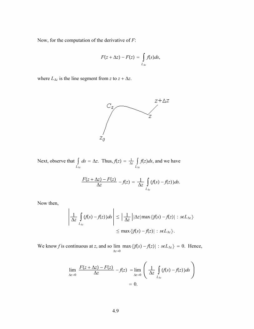
Now, for the computation of the derivative of F:

Fz z Fz Lz

fsds,

where Lz is the line segment from z to z z.

Next, observe that Lzds z. Thus, fz 1

z Lzfzds, and we have

Fz z Fzz fz 1

z Lz

fs fzds.

Now then,

1z

Lz

fs fzds 1z |z|max|fs fz| : sLz

max|fs fz| : sLz.

We know f is continuous at z, and soz0lim max|fs fz| : sLz 0. Hence,

z0lim Fz z Fz

z fz z0lim 1

z Lz

fs fzds

0.

4.9

In other words, F z fz, and so, just as promised, f has an antiderivative! Let’ssummarize what we have shown in this section:

Suppose f : D C is continuous, where D is connected and every point of D is an interiorpoint. Then f has an antiderivative if and only if the integral between any two points of D ispath independent.

Exercises

7. Suppose C is any curve from 0 to 2i. Evaluate the integral

C

cos z2 dz.

8. a)Let Fz log z, 0 arg z 2. Show that the derivative F z 1z .

b)Let Gz log z, 4 arg z 7

4 . Show that the derivative Gz 1

z .c)Let C1 be a curve in the right-half plane D1 z : Re z 0 from i to i that does not

pass through the origin. Find the integral

C1

1z dz.

d)Let C2 be a curve in the left-half plane D2 z : Re z 0 from i to i that does notpass through the origin. Find the integral.

C2

1z dz.

9. Let C be the circle of radius 1 centered at 0 with the clockwise orientation. Find

C

1z dz.

10. a)Let Hz zc, arg z . Find the derivative Hz.b)Let Kz zc,

4 arg z 74 . What is the largest subset of the plane on which

Hz Kz?c)Let C be any path from 1 to 1 that lies completely in the upper half-plane. (Upper

4.10

half-plane z : Im z 0.) Find

C

Fzdz,

where Fz zi, arg z .

11. Suppose P is a polynomial and C is a closed curve. Explain how you know thatCPzdz 0.

4.11

Chapter Five

Cauchy’s Theorem

5.1. Homotopy. Suppose D is a connected subset of the plane such that every point of D isan interior point—we call such a set a region—and let C1 and C2 be oriented closed curvesin D. We say C1 is homotopic to C2 in D if there is a continuous function H : S D,where S is the square S t, s : 0 s, t 1, such that Ht, 0 describes C1 and Ht, 1describes C2, and for each fixed s, the function Ht, s describes a closed curve Cs in D.The function H is called a homotopy between C1 and C2. Note that if C1 is homotopic toC2 in D, then C2 is homotopic to C1 in D. Just observe that the functionKt, s Ht, 1 s is a homotopy.

It is convenient to consider a point to be a closed curve. The point c is a described by aconstant function t c. We thus speak of a closed curve C being homotopic to aconstant—we sometimes say C is contractible to a point.

Emotionally, the fact that two closed curves are homotopic in D means that one can becontinuously deformed into the other in D.

Example

Let D be the annular region D z : 1 |z| 5. Suppose C1 is the circle described by1t 2ei2t, 0 t 1; and C2 is the circle described by 2t 4ei2t, 0 t 1. ThenHt, s 2 2sei2t is a homotopy in D between C1 and C2. Suppose C3 is the samecircle as C2 but with the opposite orientation; that is, a description is given by3t 4ei2t, 0 t 1. A homotopy between C1 and C3 is not too easy to construct—infact, it is not possible! The moral: orientation counts. From now on, the term ”closedcurve” will mean an oriented closed curve.

5.1

Another Example

Let D be the set obtained by removing the point z 0 from the plane. Take a look at thepicture. Meditate on it and convince yourself that C and K are homotopic in D, but and are homotopic in D, while K and are not homotopic in D.

Exercises

1. Suppose C1 is homotopic to C2 in D, and C2 is homotopic to C3 in D. Prove that C1 ishomotopic to C3 in D.

2. Explain how you know that any two closed curves in the plane C are homotopic in C.

3. A region D is said to be simply connected if every closed curve in D is contractible to apoint in D. Prove that any two closed curves in a simply connected region are homotopic inD.

5.2 Cauchy’s Theorem. Suppose C1 and C2 are closed curves in a region D that arehomotopic in D, and suppose f is a function analytic on D. Let Ht, s be a homotopybetween C1 and C2. For each s, the function st describes a closed curve Cs in D. LetIs be given by

Is Cs

fzdz.

Then,

5.2

Is 0

1

fHt, s Ht, st dt.

Now let’s look at the derivative of Is. We assume everything is nice enough to allow usto differentiate under the integral:

Is dds

0

1

fHt, s Ht, st dt

0

1

f Ht, s Ht, ss

Ht, st fHt, s

2Ht, sst dt

0

1

f Ht, s Ht, ss

Ht, st fHt, s

2Ht, sts dt

0

1t fHt, s Ht, s

s dt

fH1, s H1, ss fH0, s H0, s

s .

But we know each Ht, s describes a closed curve, and so H0, s H1, s for all s. Thus,

Is fH1, s H1, ss fH0, s H0, s

s 0,

which means Is is constant! In particular, I0 I1, or

C1

fzdz C2

fzdz.

This is a big deal. We have shown that if C1 and C2 are closed curves in a region D that arehomotopic in D, and f is analytic on D, then

C1

fzdz C2

fzdz.

An easy corollary of this result is the celebrated Cauchy’s Theorem, which says that if f isanalytic on a simply connected region D, then for any closed curve C in D,

5.3

C

fzdz 0.

In court testimony, one is admonished to tell the truth, the whole truth, and nothing but thetruth. Well, so far in this chapter, we have told the truth and nothing but the truth, but wehave not quite told the whole truth. We assumed all sorts of continuous derivatives in thepreceding discussion. These are not always necessary—specifically, the results can beproved true without all our smoothness assumptions—think about approximation.

Example

Look at the picture below and convince your self that the path C is homotopic to the closedpath consisting of the two curves C1 and C2 together with the line L. We traverse the linetwice, once from C1 to C2 and once from C2 to C1.

Observe then that an integral over this closed path is simply the sum of the integrals overC1 and C2, since the two integrals along L , being in opposite directions, would sum tozero. Thus, if f is analytic in the region bounded by these curves (the region with two holesin it), then we know that

C

fzdz C1

fzdz C2

fzdz.

Exercises

4. Prove Cauchy’s Theorem.

5. Let S be the square with sides x 100, and y 100 with the counterclockwiseorientation. Find

5.4

S

1z dz.

6. a)Find C

1z1 dz, where C is any circle centered at z 1 with the usual counterclockwise

orientation: t 1 Ae2it, 0 t 1.b)Find

C

1z1 dz, where C is any circle centered at z 1 with the usual counterclockwise

orientation.

c)Find C

1z21

dz, where C is the ellipse 4x2 y2 100 with the counterclockwise

orientation. [Hint: partial fractions]

d)Find C

1z21

dz, where C is the circle x2 10x y2 0 with the counterclockwise

orientation.

8. Evaluate CLog z 3dz, where C is the circle |z| 2 oriented counterclockwise.

9. Evaluate C

1zn dz where C is the circle described by t e

2it, 0 t 1, and n is an

integer 1.

10. a)Does the function fz 1z have an antiderivative on the set of all z 0? Explain.

b)How about fz 1zn , n an integer 1 ?

11. Find as large a set D as you can so that the function fz ez2 have an antiderivativeon D.

12. Explain how you know that every function analytic in a simply connected (cf. Exercise3) region D is the derivative of a function analytic in D.

5.5

Chapter Six

More Integration

6.1. Cauchy’s Integral Formula. Suppose f is analytic in a region containing a simpleclosed contour C with the usual positive orientation and its inside , and suppose z0 is insideC. Then it turns out that

fz0 12i

C

fzz z0 dz.

This is the famous Cauchy Integral Formula. Let’s see why it’s true.

Let 0 be any positive number. We know that f is continuous at z0 and so there is anumber such that |fz fz0| whenever |z z0 | . Now let 0 be a numbersuch that and the circle C0 z : |z z0 | is also inside C. Now, the functionfzzz0 is analytic in the region between C and C0; thus

C

fzz z0 dz

C0

fzz z0 dz.

We know that C0

1zz0 dz 2i, so we can write

C0

fzz z0 dz 2ifz0

C0

fzz z0 dz fz0

C0

1z z0 dz

C0

fz fz0z z0 dz.

For zC0 we havefz fz0z z0 |fz fz0|

|z z0 | .

Thus,

6.1

C0

fzz z0 dz 2ifz0

C0

fz fz0z z0 dz

2 2.

But is any positive number, and so

C0

fzz z0 dz 2ifz0 0,

or,

fz0 12i

C0

fzz z0 dz

12i

C

fzz z0 dz,

which is exactly what we set out to show.

Meditate on this result. It says that if f is analytic on and inside a simple closed curve andwe know the values fz for every z on the simple closed curve, then we know the value forthe function at every point inside the curve—quite remarkable indeed.

Example

Let C be the circle |z| 4 traversed once in the counterclockwise direction. Let’s evaluatethe integral

C

cos zz2 6z 5

dz.

We simply write the integrand as

cos zz2 6z 5

cos zz 5z 1 fz

z 1 ,

wherefz cos z

z 5 .

Observe that f is analytic on and inside C, and so,

6.2

C

cos zz2 6z 5

dz C

fzz 1 dz 2if1

2i cos11 5 i2 cos1

Exercises

1. Suppose f and g are analytic on and inside the simple closed curve C, and supposemoreover that fz gz for all z on C. Prove that fz gz for all z inside C.

2. Let C be the ellipse 9x2 4y2 36 traversed once in the counterclockwise direction.Define the function g by

gz C

s2 s 1s z ds.

Find a) gi b) g4i

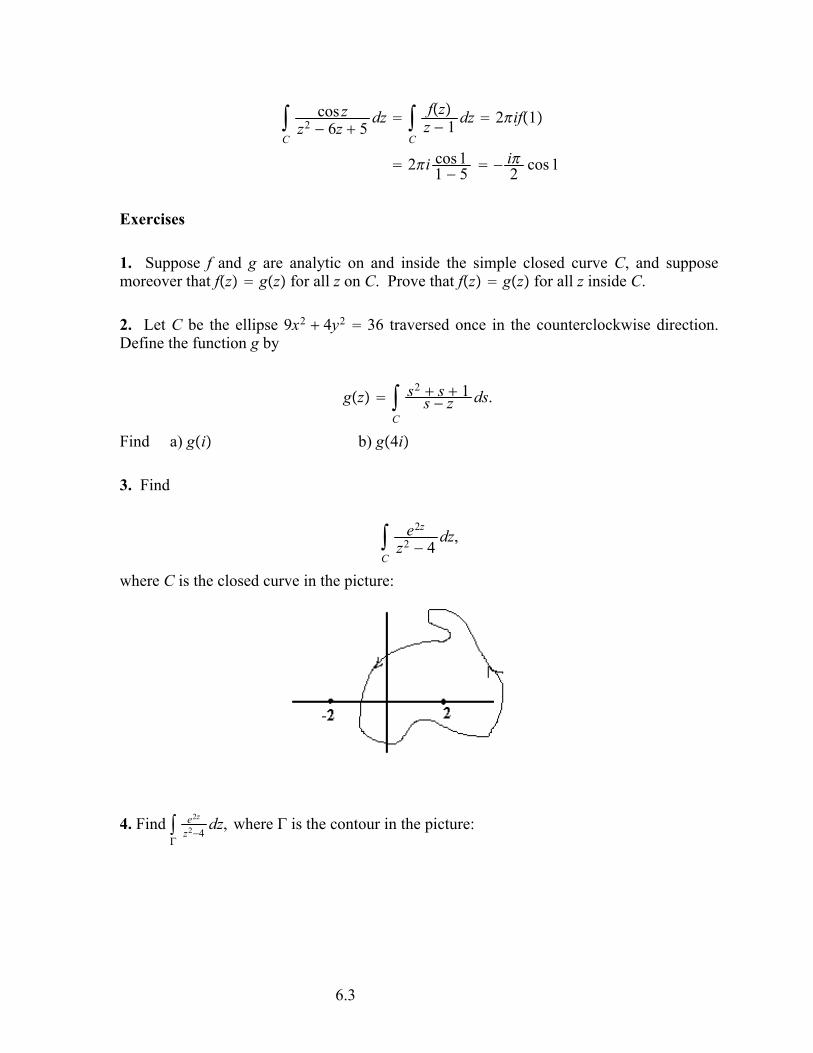
3. Find

C

e2zz2 4

dz,

where C is the closed curve in the picture:

4. Find

e2zz24

dz, where is the contour in the picture:

6.3

6.2. Functions defined by integrals. Suppose C is a curve (not necessarily a simple closedcurve, just a curve) and suppose the function g is continuous on C (not necessarily analytic,just continuous). Let the function G be defined by

Gz C

gss z ds

for all z C. We shall show that G is analytic. Here we go.

Consider,Gz z Gz

z 1z

C

1s z z

1s z gsds

C

gss z zs z ds.

Next,

Gz z Gzz

C

gss z2

ds C

1s z zs z

1s z2

gsds

C

s z s z zs z zs z2

gsds

z C

gss z zs z2

ds.

Now we want to show that

6.4

z0lim z

C

gss z zs z2

ds 0.

To that end, let M max|gs| : s C, and let d be the shortest distance from z to C.Thus, for s C, we have |s z| d 0 and also

|s z z| |s z| |z| d |z|.

Putting this all together, we can estimate the integrand above:

gss z zs z2

Md |z|d2

for all s C. Finally,

z C

gss z zs z2

ds |z| Md |z|d2

lengthC,

and it is clear that

z0lim z

C

gss z zs z2

ds 0,

just as we set out to show. Hence G has a derivative at z, and

Gz C

gss z2

ds.

Truly a miracle!

Next we see that G has a derivative and it is just what you think it should be. Consider

6.5

Gz z Gzz 1

z C

1s z z2

1s z2

gsds

1z

C

s z2 s z z2s z z2s z2

gsds

1z

C

2s zz z2s z z2s z2

gsds

C

2s z zs z z2s z2

gsds

Next,

Gz z Gzz 2

C

gss z3

ds

C

2s z zs z z2s z2

2s z3

gsds

C

2s z2 zs z 2s z z2s z z2s z3

gsds

C

2s z2 zs z 2s z2 4zs z 2z2s z z2s z3

gsds

C

3zs z 2z2s z z2s z3

gsds

Hence,

Gz z Gzz 2

C

gss z3

ds C

3zs z 2z2s z z2s z3

gsds

|z| |3m| 2|z|Md z2d3

,

where m max|s z| : s C. It should be clear then that

z0lim Gz z Gz

z 2 C

gss z3

ds 0,

or in other words,

6.6

Gz 2 C

gss z3

ds.

Suppose f is analytic in a region D and suppose C is a positively oriented simple closedcurve in D. Suppose also the inside of C is in D. Then from the Cauchy Integral formula,we know that

2ifz C

fss z ds

and so with g f in the formulas just derived, we have

f z 12i

C

fss z2

ds, and f z 22i

C

fss z3

ds

for all z inside the closed curve C. Meditate on these results. They say that the derivativeof an analytic function is also analytic. Now suppose f is continuous on a domain D inwhich every point of D is an interior point and suppose that

Cfzdz 0 for every closed

curve in D. Then we know that f has an antiderivative in D—in other words f is thederivative of an analytic function. We now know this means that f is itself analytic. Wethus have the celebratedMorera’s Theorem:

If f:D C is continuous and such that Cfzdz 0 for every closed curve in D, then f is

analytic in D.

Example

Let’s evaluate the integral

C

ezz3dz,

where C is any positively oriented closed curve around the origin. We simply use theequation

f z 22i

C

fss z3

ds

6.7

with z 0 and fs es.Thus,

ie0 i C

ezz3dz.

Exercises

5. Evaluate

C

sin zz2dz

where C is a positively oriented closed curve around the origin.

6. Let C be the circle |z i| 2 with the positive orientation. Evaluate

a) C

1z24

dz b) C

1z242

dz

7. Suppose f is analytic inside and on the simple closed curve C. Show that

C

f zz w dz

C

fzz w2

dz

for every w C.

8. a) Let be a real constant, and let C be the circle t eit, t . Evaluate

C

ezz dz.

b) Use your answer in part a) to show that

0

ecos t cos sin tdt .

6.3. Liouville’s Theorem. Suppose f is entire and bounded; that is, f is analytic in theentire plane and there is a constant M such that |fz| M for all z. Then it must be truethat f z 0 identically. To see this, suppose that f w 0 for some w. Choose R largeenough to insure that M

R |f w|. Now let C be a circle centered at 0 and with radius

6.8

maxR, |w|. Then we have :

M |f w| 1

2i C

fss w2

dz

12

M22 M

,

a contradiction. It must therefore be true that there is no w for which f w 0; or, in otherwords, f z 0 for all z. This, of course, means that f is a constant function. What wehave shown has a name, Liouville’s Theorem:

The only bounded entire functions are the constant functions.

Let’s put this theorem to some good use. Let pz anzn an1zn1 a1z a0 be apolynomial. Then

pz an an1z an2z2

a0zn zn.

Now choose R large enough to insure that for each j 1,2, ,n, we have anjzj

|an |2n

whenever |z| R. (We are assuming that an 0. ) Hence, for |z| R, we know that

|pz| |an | an1z an2

z2 a0zn |z|n

|an | an1z an2

z2 a0

zn |z|n

|an | |an |2n

|an |2n

|an |2n |z|n

|an |2 |z|n.

Hence, for |z| R,

1pz 2

|an ||z|n 2|an |Rn

.

Now suppose pz 0 for all z. Then 1pz is also bounded on the disk |z| R. Thus,

1pz

is a bounded entire function, and hence, by Liouville’s Theorem, constant! Hence thepolynomial is constant if it has no zeros. In other words, if pz is of degree at least one,there must be at least one z0 for which pz0 0. This is, of course, the celebrated

6.9

Fundamental Theorem of Algebra.

Exercises

9. Suppose f is an entire function, and suppose there is an M such that Re fz M for allz. Prove that f is a constant function.

10. Suppose w is a solution of 5z4 z3 z2 7z 14 0. Prove that |w| 3.

11. Prove that if p is a polynomial of degree n, and if pa 0, then pz z aqz,where q is a polynomial of degree n 1.

12. Prove that if p is a polynomial of degree n 1, then

pz cz z1k1z z2k2 z zjkj ,

where k1,k2, ,kj are positive integers such that n k1 k2 kj.

13. Suppose p is a polynomial with real coefficients. Prove that p can be expressed as aproduct of linear and quadratic factors, each with real coefficients.

6.4. Maximum moduli. Suppose f is analytic on a closed domain D. Then, beingcontinuous, |fz| must attain its maximum value somewhere in this domain. Suppose thishappens at an interior point. That is, suppose |fz| M for all z D and suppose that|fz0| M for some z0 in the interior of D. Now z0 is an interior point of D, so there is anumber R such that the disk centered at z0 having radius R is included in D. Let C be apositively oriented circle of radius R centered at z0. From Cauchy’s formula, weknow

fz0 12i

C

fss z0 ds.

Hence,

fz0 12

0

2

fz0 eitdt,

and so,

6.10

M |fz0| 12

0

2

|fz0 eit|dt M.

since |fz0 eit| M. This means

M 12

0

2

|fz0 eit|dt.

Thus,

M 12

0

2

|fz0 eit|dt 12

0

2

M |fz0 eit|dt 0.

This integrand is continuous and non-negative, and so must be zero. In other words,|fz| M for all z C. There was nothing special about C except its radius R, and sowe have shown that f must be constant on the disk .

I hope it is easy to see that if D is a region (connected and open), then the only way inwhich the modulus |fz| of the analytic function f can attain a maximum on D is for f to beconstant.

Exercises

14. Suppose f is analytic and not constant on a region D and suppose fz 0 for all z D.Explain why |fz| does not have a minimum in D.

15. Suppose fz ux,y ivx,y is analytic on a region D. Prove that if ux,y attains amaximum value in D, then u must be constant.

6.11

Chapter Seven

Harmonic Functions

7.1. The Laplace equation. The Fourier law of heat conduction says that the rate at whichheat passes across a surface S is proportional to the flux, or surface integral, of thetemperature gradient on the surface:

k S

T dA.

Here k is the constant of proportionality, generally called the thermal conductivity of thesubstance (We assume uniform stuff. ). We further assume no heat sources or sinks, and weassume steady-state conditions—the temperature does not depend on time. Now if we takeS to be an arbitrary closed surface, then this rate of flow must be 0:

k S

T dA 0.

Otherwise there would be more heat entering the region B bounded by S than is comingout, or vice-versa. Now, apply the celebrated Divergence Theorem to conclude that

B

TdV 0,

where B is the region bounded by the closed surface S. But since the region B is completelyarbitrary, this means that

T 2Tx2

2Ty2

2Tz2

0.

This is the world-famous Laplace Equation.

Now consider a slab of heat conducting material,

7.1

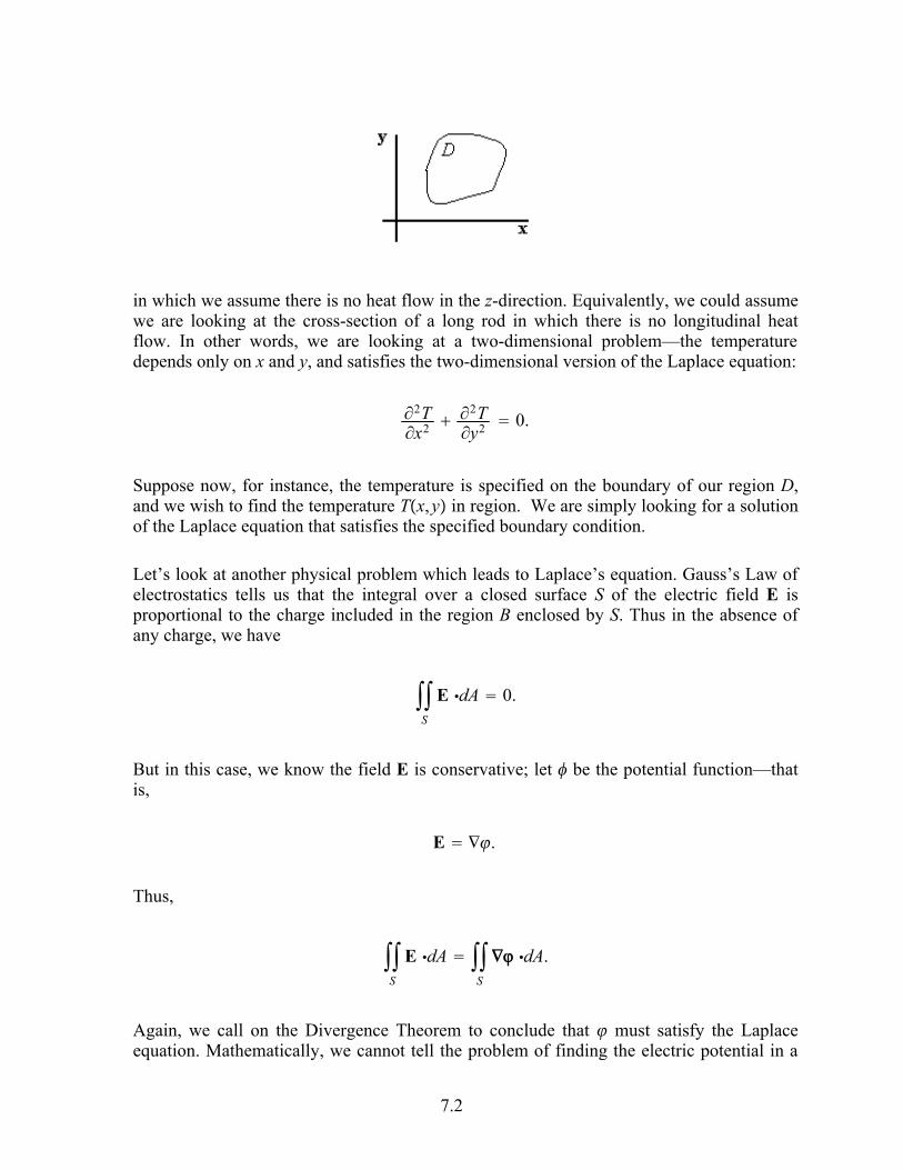
in which we assume there is no heat flow in the z-direction. Equivalently, we could assumewe are looking at the cross-section of a long rod in which there is no longitudinal heatflow. In other words, we are looking at a two-dimensional problem—the temperaturedepends only on x and y, and satisfies the two-dimensional version of the Laplace equation:

2Tx2

2Ty2

0.

Suppose now, for instance, the temperature is specified on the boundary of our region D,and we wish to find the temperature Tx,y in region. We are simply looking for a solutionof the Laplace equation that satisfies the specified boundary condition.

Let’s look at another physical problem which leads to Laplace’s equation. Gauss’s Law ofelectrostatics tells us that the integral over a closed surface S of the electric field E isproportional to the charge included in the region B enclosed by S. Thus in the absence ofany charge, we have

S

E dA 0.

But in this case, we know the field E is conservative; let be the potential function—thatis,

E .

Thus,

S

E dA S

dA.

Again, we call on the Divergence Theorem to conclude that must satisfy the Laplaceequation. Mathematically, we cannot tell the problem of finding the electric potential in a

7.2

region D, given the potential on the boundary of D, from the previous problem of findingthe temperature in the region, given the temperature on the boundary. These are but two ofthe many physical problems that lead to the Laplace equation—You probably already knowof some others. Let D be a domain and let be a given function continuous on theboundary of D. The problem of finding a function harmonic on the interior of D andwhich agrees with on the boundary of D is called the Dirichlet problem.

7.2. Harmonic functions. If D is a region in the plane, a real-valued function ux,yhaving continuous second partial derivatives is said to be harmonic on D if it satisfiesLaplace’s equation on D :

2ux2

2uy2

0.

There is an intimate relationship between harmonic functions and analytic functions.Suppose f is analytic on D, and let fz ux,y ivx,y. Now, from the Cauchy-Riemannequations, we know

ux v

y , and

uy v

x .

If we differentiate the first of these with respect to x and the second with respect to y, andthen add the two results, we have

2ux2

2uy2

2vxy

2vyx 0.

Thus the real part of any analytic function is harmonic! Next, if we differentiate the first ofthe Cauchy-Riemann equations with respect to y and the second with respect to x, and thensubtract the second from the first, we have

2vx2

2vy2

0,

and we see that the imaginary part of an analytic function is also harmonic.

There is even more excitement. Suppose we are given a function harmonic in a simplyconnected region D. Then there is a function f analytic on D which is such that Re f .Let’s see why this is so. First, define g by

7.3

gz x i

y .

We’ll show that g is analytic by verifying that the real and imaginary parts satisfy theCauchy-Riemann equations:

x

x

2x2

2y2

y

y ,

since is harmonic. Next,

y

x 2

yx 2xy

x y .

Since g is analytic on the simply connected region D, we know that the integral of g aroundany closed curve is zero, and so it has an antiderivative Gz u iv. This antiderivativeis, of course, analytic on D, and we know that

Gz ux i

uy

x iy .

Thus, ux,y x,y hy. From this,

uy

y hy,

and so hy 0, or h constant, from which it follows that ux,y x,y c. In otherwords, ReG u, as we promised to show.

Example

The function x,y x3 3xy2 is harmonic everywhere. We shall find an analyticfunction G so that ReG . We know that Gz x3 3xy2 iv, and so from theCauchy-Riemann equations:

vx u

y 6xy

7.4

Hence,

vx,y 3x2y ky.

To find ky differentiate with respect to y :

vy 3x2 k y u

x 3x2 3y2,

and so,

k y 3y2, orky y3 any constant.

If we choose the constant to be zero, this gives us

v 3x2y ky 3x2y y3,

and finally,

Gz u iv x3 3xy2 i3x2y y3.

Exercises

1. Suppose is harmonic on a simply connected region D. Prove that if assumes itsmaximum or its minimum value at some point in D, then is constant in D.

2. Suppose and are harmonic in a simply connected region D bounded by the curve C.Suppose moreover that x,y x,y for all x,y C. Explain how you know that everywhere in D.

3. Find an entire function f such that Re f x2 3x y2, or explain why there is no suchfunction f.

4. Find an entire function f such that Re f x2 3x y2, or explain why there is no suchfunction f.

7.5

7.3. Poisson’s integral formula. Let be the disk bounded by the circleC z : |z| . Suppose is harmonic on and let f be a function analytic on andsuch that Re f . Now then, for fixed z with |z| , the function

gs fs z2 s z

is analyic on . Thus from Cauchy’s Theorem

C

gsds C

fs z2 s z

ds 0.

We know also that

fz 12i

C

fss z ds.

Adding these two equations gives us

fz 12i

C

1s z

z2 s z

fsds

12i

C

2 |z|2

s z2 s z fsds.

Next, let t eit, and our integral becomes

fz 12i

0

22 |z|2

eit z2 eit z feitieitdt

2 |z|22

0

2feit

eit zeit z dt

2 |z|22

0

2feit|eit z|2

dt

Now,

7.6

x,y Re f 2 |z|22

0

2eit|eit z|2

dt.

Next, use polar coordinates: z rei :

r, 2 r22

0

2eit

|eit rei |2dt.

Now,

|eit rei |2 eit reieit rei 2 r2 reit eit 2 r2 2rcost .

Substituting this in the integral, we have Poisson’s integral formula:

r, 2 r22

0

2eit

2 r2 2rcost dt

This famous formula essentially solves the Dirichlet problem for a disk.

Exercises

5. Evaluate 0

21

2r22rcostdt. [Hint: This is easy.]

6. Suppose is harmonic in a region D. If x0,y0 D and if C D is a circle centered atx0,y0, the inside of which is also in D, then x0,y0 is the average value of on thecircle C.

7. Suppose is harmonic on the disk z : |z| . Prove that

0,0 12

dA.

7.7

Chapter Eight

Series

8.1. Sequences. The basic definitions for complex sequences and series are essentially thesame as for the real case. A sequence of complex numbers is a function g : Z C fromthe positive integers into the complex numbers. It is traditional to use subscripts to indicatethe values of the function. Thus we write gn zn and an explicit name for the sequenceis seldom used; we write simply zn to stand for the sequence g which is such thatgn zn. For example, in is the sequence g for which gn i

n .

The number L is a limit of the sequence zn if given an 0, there is an integer N suchthat |zn L| for all n N. If L is a limit of zn, we sometimes say that znconverges to L. We frequently write limzn L. It is relatively easy to see that if thecomplex sequence zn un ivn converges to L, then the two real sequences un andvn each have a limit: un converges to ReL and vn converges to ImL. Conversely, ifthe two real sequences un and vn each have a limit, then so also does the complexsequence un ivn. All the usual nice properties of limits of sequences are thus true:

limzn wn limzn limwn;limznwn limzn limwn; and

lim znwn limzn

limwn.

provided that limzn and limwn exist. (And in the last equation, we must, of course,insist that limwn 0.)

A necessary and sufficient condition for the convergence of a sequence an is thecelebrated Cauchy criterion: given 0, there is an integer N so that |an am | whenever n,m N.

A sequence fn of functions on a domain D is the obvious thing: a function from thepositive integers into the set of complex functions on D. Thus, for each zD, we have anordinary sequence fnz. If each of the sequences fnz converges, then we say thesequence of functions fn converges to the function f defined by fz limfnz. Thispretty obvious stuff. The sequence fn is said to converge to f uniformly on a set S ifgiven an 0, there is an integer N so that |fnz fz| for all n N and all z S.

Note that it is possible for a sequence of continuous functions to have a limit function thatis not continuous. This cannot happen if the convergence is uniform. To see this, supposethe sequence fn of continuous functions converges uniformly to f on a domain D, letz0D, and let 0. We need to show there is a so that |fz0 fz| whenever

8.1

|z0 z| . Let’s do it. First, choose N so that |fNz fz| 3 . We can do this because

of the uniform convergence of the sequence fn. Next, choose so that|fNz0 fNz|

3 whenever |z0 z| . This is possible because fN is continuous.Now then, when |z0 z| , we have

|fz0 fz| |fz0 fNz0 fNz0 fNz fNz fz| |fz0 fNz0| |fNz0 fNz| |fNz fz| 3

3 3 ,

and we have done it!

Now suppose we have a sequence fn of continuous functions which converges uniformly

on a contour C to the function f. Then the sequence Cfnzdz converges to

Cfzdz. This

is easy to see. Let 0. Now let N be so that |fnz fz| A for n N, where A is the

length of C. Then,

C

fnzdz C

fzdz C

fnz fzdz

A A

whenever n N.

Now suppose fn is a sequence of functions each analytic on some region D, and supposethe sequence converges uniformly on D to the function f. Then f is analytic. This result is inmarked contrast to what happens with real functions—examples of uniformly convergentsequences of differentiable functions with a nondifferentiable limit abound in the real case.To see that this uniform limit is analytic, let z0D, and let S z : |z z0 | r D . Nowconsider any simple closed curve C S. Each fn is analytic, and so

Cfnzdz 0 for every

n. From the uniform convergence of fn , we know that Cfzdz is the limit of the sequence

Cfnzdz , and so

Cfzdz 0. Morera’s theorem now tells us that f is analytic on S, and

hence at z0. Truly a miracle.

Exercises

8.2

1. Prove that a sequence cannot have more than one limit. (We thus speak of the limit of asequence.)

2. Give an example of a sequence that does not have a limit, or explain carefully why thereis no such sequence.

3. Give an example of a bounded sequence that does not have a limit, or explain carefullywhy there is no such sequence.

4. Give a sequence fn of functions continuous on a set D with a limit that is notcontinuous.

5. Give a sequence of real functions differentiable on an interval which convergesuniformly to a nondifferentiable function.

8.2 Series. A series is simply a sequence sn in which sn a1 a2 an. In otherwords, there is sequence an so that sn sn1 an. The sn are usually called the partial

sums. Recall from Mrs. Turner’s class that if the series j1

naj has a limit, then it must be

true thatnlim an 0.

Consider a series j1

nfjz of functions. Chances are this series will converge for some

values of z and not converge for others. A useful result is the celebrated WeierstrassM-test: Suppose Mj is a sequence of real numbers such that Mj 0 for all j J, where

J is some number., and suppose also that the series j1

nMj converges. If for all zD, we

have |fjz| Mj for all j J, then the series j1

nfjz converges uniformly on D.

To prove this, begin by letting 0 and choosing N J so that

jm

n

Mj

for all n,m N. (We can do this because of the famous Cauchy criterion.) Next, observethat

8.3

jm

n

fjz jm

n

|fjz| jm

n

Mj .

This shows that j1

nfjz converges. To see the uniform convergence, observe that

jm

n

fjz j0

n

fjz j0

m1

fjz

for all zD and n m N. Thus,

nlim

j0

n

fjz j0

m1

fjz j0

fjz j0

m1

fjz

for m N.(The limit of a series j0

naj is almost always written as

j0

aj.)

Exercises

6. Find the set D of all z for which the sequence znzn3n has a limit. Find the limit.

7. Prove that the series j1

naj convegres if and only if both the series

j1

nReaj and

j1

nImaj converge.

8. Explain how you know that the series j1

n 1z

j converges uniformly on the set

|z| 5.

8.3 Power series. We are particularly interested in series of functions in which the partialsums are polynomials of increasing degree:

snz c0 c1z z0 c2z z02 cnz z0n.

8.4

(We start with n 0 for esthetic reasons.) These are the so-called power series. Thus,

a power series is a series of functions of the form j0

ncjz z0 j .

Let’s look first as a very special power series, the so-called Geometric series:

j0

n

zj .

Heresn 1 z z2 zn, andzsn z z2 z3 zn1.

Subtracting the second of these from the first gives us

1 zsn 1 zn1.

If z 1, then we can’t go any further with this, but I hope it’s clear that the series does nothave a limit in case z 1. Suppose now z 1. Then we have

sn 11 z

zn11 z .

Now if |z| 1, it should be clear that limzn1 0, and so

lim j0

n

zj lim sn 11 z .

Or,

j0

zj 11 z , for |z| 1.

There is a bit more to the story. First, note that if |z| 1, then the Geometric series doesnot have a limit (why?). Next, note that if |z| 1, then the Geometric series converges

8.5

uniformly to 11z . To see this, note that

j0

n

j

has a limit and appeal to the Weierstrass M-test.

Clearly a power series will have a limit for some values of z and perhaps not for others.First, note that any power series has a limit when z z0. Let’s see what else we can say.

Consider a power series j0

ncjz z0 j . Let

lim sup j |cj | .

(Recall from 6th grade that lim supak limsupak : k n. ) Now let R 1 . (We

shall say R 0 if , and R if 0. ) We are going to show that the seriesconverges uniformly for all |z z0 | R and diverges for all |z z0 | R.

First, let’s show the series does not converge for |z z0 | R. To begin, let k be so that

1|z z0 |

k 1R .

There are an infinite number of cj for which j |cj | k, otherwise lim sup j |cj | k. Foreach of these cj we have

|cjz z0 j | j |cj | |z z0 |j k|z z0 | j 1.

It is thus not possible fornlim |cnz z0n | 0, and so the series does not converge.

Next, we show that the series does converge uniformly for |z z0 | R. Let k be sothat

1R k 1

.

Now, for j large enough, we have j |cj | k. Thus for |z z0 | , we have

8.6

|cjz z0 j | j |cj | |z z0 |j k|z z0 | j k j.

The geometric series j0

nk j converges because k 1 and the uniform convergence

of j0

ncjz z0 j follows from the M-test.

Example

Consider the series j0

n1j! z

j . Let’s compute R 1/ lim sup j |cj | lim sup j j! . Let

K be any positive integer and choose an integer m large enough to insure that 2m K2K2K! .

Now consider n!Kn , where n 2K m:

n!Kn 2K m!

K2Km 2K m2K m 1 2K 12K!

KmK2K

2m 2K!K2K

1

Thus n n! K. Reflect on what we have just shown: given any number K, there is anumber n such that n n! is bigger than it. In other words, R lim sup j j! , and so the

series j0

n1j! z

j converges for all z.

Let’s summarize what we have. For any power series j0

ncjz z0 j , there is a number

R 1lim sup j |cj |

such that the series converges uniformly for |z z0 | R and does not

converge for |z z0 | R. (Note that we may have R 0 or R .) The number R iscalled the radius of convergence of the series, and the set |z z0 | R is called the circleof convergence. Observe also that the limit of a power series is a function analytic insidethe circle of convergence (why?).

Exercises

9. Suppose the sequence of real numbers j has a limit. Prove that

8.7

lim sup j lim j.

For each of the following, find the set D of points at which the series converges:

10. j0

nj!zj .

11. j0

njzj .

12. j0

nj2

3jzj .

13. j0

n1j

22jj!2z2j

8.4 Integration of power series. Inside the circle of convergence, the limit

Sz j0

cjz z0 j

is an analytic function. We shall show that this series may be integrated”term-by-term”—that is, the integral of the limit is the limit of the integrals. Specifically, ifC is any contour inside the circle of convergence, and the function g is continuous on C,then

C

gzSzdz j0

cj C

gzz z0 jdz.

Let’s see why this. First, let 0. Let M be the maximum of |gz| on C and let L be thelength of C. Then there is an integer N so that

jn

cjz z0 j ML

8.8

for all n N. Thus,

C

gzjn

cjz z0 j dz ML ML ,

Hence,

C

gzSzdz j0

n1

cj C

gzz z0 jdz C

gzjn

cjz z0 j dz

,

and we have shown what we promised.

8.5 Differentiation of power series. Again, let

Sz j0

cjz z0 j.

Now we are ready to show that inside the circle of convergence,

Sz j1

jcjz z0 j1.

Let z be a point inside the circle of convergence and let C be a positive oriented circlecentered at z and inside the circle of convergence. Define

gs 12is z2

,

and apply the result of the previous section to conclude that

8.9

C

gsSsds j0

cj C

gss z0 jds, or

12i

C

Sss z2

ds j0

cj C

s z0 js z2

ds. Thus

Sz j0

jcjz z0 j1,

as promised!

Exercises

14. Find the limit of

j0

n

j 1zj .

For what values of z does the series converge?

15. Find the limit of

j1

nzjj .

For what values of z does the series converge?

16. Find a power series j0

ncjz 1 j such that

1z

j0

cjz 1 j, for |z 1| 1.

17. Find a power series j0

ncjz 1 j such that

8.10

Log z j0

cjz 1 j, for |z 1| 1.

8.11

Chapter Nine

Taylor and Laurent Series

9.1. Taylor series. Suppose f is analytic on the open disk |z z0 | r. Let z be any point inthis disk and choose C to be the positively oriented circle of radius , where|z z0 | r. Then for sC we have

1s z 1

s z0 z z0 1s z0

11 zz0

sz0

j0

z z0 j

s z0 j1

since | zz0sz0 | 1. The convergence is uniform, so we may integrate

C

fss z ds

j0

C

fss z0 j1

ds z z0 j, or

fz 12i

C

fss z ds

j0

12i

C

fss z0 j1

ds z z0 j.

We have thus produced a power series having the given analytic function as a limit:

fz j0

cjz z0 j, |z z0 | r,

where

cj 12i

C

fss z0 j1

ds.

This is the celebrated Taylor Series for f at z z0.

We know we may differentiate the series to get

f z j1

jcjz z0 j1

9.1

and this one converges uniformly where the series for f does. We can thus differentiateagain and again to obtain

fnz jn

jj 1j 2 j n 1cjz z0 jn.

Hence,

fnz0 n!cn, or

cn fnz0n! .

But we also know that

cn 12i

C

fss z0n1

ds.

This gives us

fnz0 n!2i

C

fss z0n1

ds, for n 0,1,2, .

This is the famous Generalized Cauchy Integral Formula. Recall that we previouslyderived this formula for n 0 and 1.

What does all this tell us about the radius of convergence of a power series? Suppose wehave

fz j0

cjz z0 j,

and the radius of convergence is R. Then we know, of course, that the limit function f isanalytic for |z z0 | R. We showed that if f is analytic in |z z0 | r, then the seriesconverges for |z z0 | r. Thus r R, and so f cannot be analytic at any point z for which|z z0 | R. In other words, the circle of convergence is the largest circle centered at z0inside of which the limit f is analytic.

9.2

Example

Let fz expz ez. Then f0 f 0 fn0 1, and the Taylor series for fat z0 0 is

ez j0

1j! z

j

and this is valid for all values of z since f is entire. (We also showed earlier that thisparticular series has an infinite radius of convergence.)

Exercises

1. Show that for all z,

ez ej0

1j! z 1

j.

2.What is the radius of convergence of the Taylor series j0

ncjzj for tanh z ?

3. Show that

11 z

j0

z i j1 i j1

for |z i| 2 .

4. If fz 11z , what is f

10i ?

5. Suppose f is analytic at z 0 and f0 f 0 f 0 0. Prove there is a function ganalytic at 0 such that fz z3gz in a neighborhood of 0.

6. Find the Taylor series for fz sin z at z0 0.

7. Show that the function f defined by

9.3

fz sin zz for z 01 for z 0

is analytic at z 0, and find f 0.

9.2. Laurent series. Suppose f is analytic in the region R1 |z z0 | R2, and let C be apositively oriented simple closed curve around z0 in this region. (Note: we include thepossiblites that R1 can be 0, and R2 .) We shall show that for z C in this region

fz j0

ajz z0 j j1

bjz z0 j

,

where

aj 12i

C

fss z0 j1

ds, for j 0,1,2,

and

bj 12i

C

fss z0j1

ds, for j 1,2, .

The sum of the limits of these two series is frequently written

fz j

cjz z0 j,

where

cj 12i

C

fss z0 j1

, j 0,1,2, .

This recipe for fz is called a Laurent series, although it is important to keep in mind thatit is really two series.

9.4

Okay, now let’s derive the above formula. First, let r1 and r2 be so thatR1 r1 |z z0 | r2 R2 and so that the point z and the curve C are included in theregion r1 |z z0 | r2. Also, let be a circle centered at z and such that is included inthis region.

Then fssz is an analytic function (of s) on the region bounded by C1,C2, and , where C1 is

the circle |z| r1 and C2 is the circle |z| r2. Thus,

C2

fss z ds

C1

fss z ds

fss z ds.

(All three circles are positively oriented, of course.) But

fssz ds 2ifz, and so we have

2ifz C2

fss z ds

C1

fss z ds.

Look at the first of the two integrals on the right-hand side of this equation. For sC2, wehave |z z0 | |s z0 |, and so

1s z 1

s z0 z z0

1s z0

11 zz0sz0

1s z0

j0

z z0s z0

j

j0

1

s z0 j1z z0 j.

9.5

Hence,

C2

fss z ds

j0

C2

fss z0 j1

ds z z0 j

.j0

C

fss z0 j1

ds z z0 j

For the second of these two integrals, note that for sC1 we have |s z0 | |z z0 |, and so

1s z 1

z z0 s z0 1z z0

11 sz0zz0

1z z0

j0

s z0z z0

j

j0

s z0 j 1z z0 j1

j1

s z0 j1 1z z0 j

j1

1

s z0j11

z z0 j

As before,

C1

fss z ds

j1

C2

fss z0j1

ds 1z z0 j

j1

C

fss z0j1

ds 1z z0 j

Putting this altogether, we have the Laurent series:

fz 12i

C2

fss z ds

12i

C1

fss z ds

j0

12i

C

fss z0 j1

ds z z0 j j1

12i

C

fss z0j1

ds 1z z0 j

.

Example

9.6

Let f be defined by

fz 1zz 1 .

First, observe that f is analytic in the region 0 |z| 1. Let’s find the Laurent series for fvalid in this region. First,

fz 1zz 1 1z 1

z 1 .

From our vast knowledge of the Geometric series, we have

fz 1z j0

zj.

Now let’s find another Laurent series for f, the one valid for the region 1 |z| .First,

1z 1 1

z1

1 1z

.

Now since | 1z | 1, we have

1z 1 1

z1

1 1z

1z

j0

zj j1

zj,

and so

fz 1z 1z 1 1z

j1

zj

fz j2

zj.

Exercises

8. Find two Laurent series in powers of z for the function f defined by

9.7

fz 1z21 z

and specify the regions in which the series converge to fz.

9. Find two Laurent series in powers of z for the function f defined by

fz 1z1 z2

and specify the regions in which the series converge to fz.

10. Find the Laurent series in powers of z 1 for fz 1z in the region 1 |z 1| .

9.8

Chapter Ten

Poles, Residues, and All That

10.1. Residues. A point z0 is a singular point of a function f if f not analytic at z0, but isanalytic at some point of each neighborhood of z0. A singular point z0 of f is said to beisolated if there is a neighborhood of z0 which contains no singular points of f save z0. Inother words, f is analytic on some region 0 |z z0 | .

Examples

The function f given by

fz 1zz2 4

has isolated singular points at z 0, z 2i, and z 2i.

Every point on the negative real axis and the origin is a singular point of Log z , but thereare no isolated singular points.

Suppose now that z0 is an isolated singular point of f . Then there is a Laurent series

fz j

cjz z0 j

valid for 0 |z z0 | R, for some positive R. The coefficient c1 of z z01 is called theresidue of f at z0, and is frequently written

zz0Res f.

Now, why do we care enough about c1to give it a special name? Well, observe that if C isany positively oriented simple closed curve in 0 |z z0 | R and which contains z0inside, then

c1 12i

C

fzdz.

10.1

This provides the key to evaluating many complex integrals.

Example

We shall evaluate the integral

C

e1/zdz

where C is the circle |z| 1 with the usual positive orientation. Observe that the integrandhas an isolated singularity at z 0. We know then that the value of the integral is simply2i times the residue of e1/z at 0. Let’s find the Laurent series about 0. We already knowthat

ez j0

1j! z

j

for all z . Thus,

e1/z j0

1j! z

j 1 1z 12!1z2

The residue c1 1, and so the value of the integral is simply 2i.

Now suppose we have a function f which is analytic everywhere except for isolatedsingularities, and let C be a simple closed curve (positively oriented) on which f is analytic.Then there will be only a finite number of singularities of f inside C (why?). Call them z1,z2, , zn. For each k 1,2, ,n, let Ck be a positively oriented circle centered at zk andwith radius small enough to insure that it is inside C and has no other singular points insideit.

10.2

Then,

C

fzdz C1

fzdz C2

fzdz Cn

fzdz

2izz1Res f 2i

zz2Res f 2i

zznRes f

2ik1

n

zzkRes f.

This is the celebrated Residue Theorem. It says that the integral of f is simply 2i timesthe sum of the residues at the singular points enclosed by the contour C.

Exercises

Evaluate the integrals. In each case, C is the positively oriented circle |z| 2.

1. Ce1/z2dz.

2. Csin 1z dz.

3. Ccos 1z dz.

4. C

1z sin 1z dz.

5. C

1z cos 1z dz.

10.3

10.2. Poles and other singularities. In order for the Residue Theorem to be of much helpin evaluating integrals, there needs to be some better way of computing theresidue—finding the Laurent expansion about each isolated singular point is a chore. Weshall now see that in the case of a special but commonly occurring type of singularity theresidue is easy to find. Suppose z0 is an isolated singularity of f and suppose that theLaurent series of f at z0 contains only a finite number of terms involving negative powersof z z0. Thus,

fz cnz z0n

cn1z z0n1

c1z z0

c0 c1z z0 .

Multiply this expression by z z0n :

z z z0nfz cn cn1z z0 c1z z0n1 .

What we see is the Taylor series at z0 for the function z z z0nfz. The coefficientof z z0n1 is what we seek, and we know that this is

n1z0n 1!

.

The sought after residue c1 is thus

c1 zz0Res f n1z0

n 1! ,

where z z z0nfz.

Example

We shall find all the residues of the function

fz ezz2z2 1

.

First, observe that f has isolated singularities at 0, and i. Let’s see about the residue at 0.Here we have

10.4

z z2fz ezz2 1

.

The residue is simply 0 :

z z2 1ez 2zezz2 12

.

Hence,

z0Res f 0 1.

Next, let’s see what we have at z i:

z z ifz ezz2z i

,

and so

ziRes fz i e

i

2i .

In the same way, we see that

ziRes f ei

2i .

Let’s find the integral C

ezz2z21

dz , where C is the contour pictured:

10.5

This is now easy. The contour is positive oriented and encloses two singularities of f; viz, iand i. Hence,

C

ezz2z2 1

dz 2iziRes f

ziRes f

2i ei

2i ei2i

2i sin1.

Miraculously easy!

There is some jargon that goes with all this. An isolated singular point z0 of f such that theLaurent series at z0 includes only a finite number of terms involving negative powers ofz z0 is called a pole. Thus, if z0 is a pole, there is an integer n so that z z z0nfzis analytic at z0, and fz0 0. The number n is called the order of the pole. Thus, in thepreceding example, 0 is a pole of order 2, while i and i are poles of order 1. (A pole oforder 1 is frequently called a simple pole.) We must hedge just a bit here. If z0 is anisolated singularity of f and there are no Laurent series terms involving negative powers ofz z0, then we say z0 is a removable singularity.

Example

Let

fz sin zz ;

then the singularity z 0 is a removable singularity:

fz 1z sin z

1z z

z33!

z55!

1 z2

3! z45!

and we see that in some sense f is ”really” analytic at z 0 if we would just define it to bethe right thing there.

A singularity that is neither a pole or removable is called an essential singularity.

Let’s look at one more labor-saving trick—or technique, if you prefer. Suppose f is afunction:

10.6

fz pzqz ,

where p and q are analytic at z0, and we have qz0 0, while qz0 0, and pz0 0.Then

fz pzqz pz0 pz0z z0

qz0z z0 qz02 z z02

,

and so

z z z0fz pz0 pz0z z0 qz0 qz0

2 z z0 .

Thus z0 is a simple pole and

zz0Res f z0 pz0

qz0.

Example

Find the integral

C

cos zez 1 dz,

where C is the rectangle with sides x 1, y , and y 3.The singularities of the integrand are all the places at which ez 1, or in other words, thepoints z 0,2i,4i, . The singularities enclosed by C are 0 and 2i. Thus,

C

cos zez 1 dz 2i z0

Res f z2iRes f ,

where

fz cos zez 1 .

10.7

Observe this is precisely the situation just discussed: fz pzqz , where p and q are

analytic, etc.,etc. Now,

pzqz

cos zez .

Thus,

z0Res f cos0

1 1,and

z2iRes f cos2i

e2i e2 e2

2 cosh2.

Finally,

C

cos zez 1 dz 2i z0

Res f z2iRes f

2i1 cosh2

Exercises

6. Suppose f has an isolated singularity at z0. Then, of course, the derivative f also has anisolated singularity at z0. Find the residue

zz0Res f .

7. Given an example of a function f with a simple pole at z0 such thatzz0Res f 0, or explain

carefully why there is no such function.

8. Given an example of a function f with a pole of order 2 at z0 such thatzz0Res f 0, or

explain carefully why there is no such function.

9. Suppose g is analytic and has a zero of order n at z0 (That is, gz z z0nhz, wherehz0 0.). Show that the function f given by

fz 1gz

10.8

has a pole of order n at z0. What iszz0Res f ?

10. Suppose g is analytic and has a zero of order n at z0. Show that the function f given by

fz gzgz

has a simple pole at z0, andzz0Res f n.

11. Find

C

cos zz2 4

dz,

where C is the positively oriented circle |z| 6.

12. Find

C

tan zdz,

where C is the positively oriented circle |z| 2.

13. Find

C

1z2 z 1

dz,

where C is the positively oriented circle |z| 10.

10.9

Chapter Eleven

Argument Principle

11.1. Argument principle. Let C be a simple closed curve, and suppose f is analytic on C.Suppose moreover that the only singularities of f inside C are poles. If fz 0 for all zC,then fC is a closed curve which does not pass through the origin. If

t, t

is a complex description of C, then

t ft, t

is a complex description of . Now, let’s compute

C

f zfz dz

f tft

tdt.

But notice that t f t t. Hence,

C

f zfz dz

f tft

tdt

tt dt

1z dz n2i,

where |n| is the number of times ”winds around” the origin. The integer n is positive incase is traversed in the positive direction, and negative in case the traversal is in thenegative direction.

Next, we shall use the Residue Theorem to evaluate the integral C

fzfz dz. The singularities

of the integrand fzfz are the poles of f together with the zeros of f. Let’s find the residues at

these points. First, let Z z1, z2, , zK be set of all zeros of f. Suppose the order of thezero zj is nj. Then fz z zjnjhz and hzj 0. Thus,

11.1

f zfz

z zjnjhz njz zjnj1hzz zjnjhz

hzhz

njz zj

.

Then

z z zj fzfz z zj h

zhz nj,

and

zzjRes f

f nj.

The sum of all these residues is thus

N n1 n2 nK.

Next, we go after the residues at the poles of f. Let the set of poles of f beP p1,p2, ,pJ. Suppose pj is a pole of order mj. Then

hz z pjmj fz

is analytic at pj. In other words,

fz hzz pjmj

.

Hence,

f zfz

z pjmjhz mjz pjmj1hzz pj2mj

z pjmjhz

hzhz

mjz pjmj

.

Now then,

11.2

z z pjmj fzfz z pjmj h

zhz mj,

and so

zpjRes f

f pj mj.

The sum of all these residues is

P m1 m2 mJ

Then,

C

f zfz dz 2iN P;

and we already found that

C

f zfz dz n2i,

where n is the ”winding number”, or the number of times winds around theorigin—n 0 means winds in the positive sense, and n negative means it winds in thenegative sense. Finally, we have

n N P,

where N n1 n2 nK is the number of zeros inside C, counting multiplicity, or theorder of the zeros, and P m1 m2 mJ is the number of poles, counting the order.This result is the celebrated argument principle.

Exercises

1. Let C be the unit circle |z| 1 positively oriented, and let f be given by

11.3

fz z3.

How many times does the curve fC wind around the origin? Explain.

2. Let C be the unit circle |z| 1 positively oriented, and let f be given by

fz z2 2z3

.

How many times does the curve fC wind around the origin? Explain.

3. Let pz anzn an1zn1 a1z a0, with an 0. Prove there is an R 0 so that ifC is the circle |z| R positively oriented, then

C

pzpz dz 2ni.

4. How many solutions of 3ez z 0 are in the disk |z| 1? Explain.

5. Suppose f is entire and fz is real if and only if z is real. Explain how you know that fhas at most one zero.

11.2 Rouche’s Theorem. Suppose f and g are analytic on and inside a simple closedcontour C. Suppose moreover that |fz| |gz| for all zC. Then we shall see that f andf g have the same number of zeros inside C. This result is Rouche’s Theorem. To seewhy it is so, start by defining the function t on the interval 0 t 1 :

t 12i

C

f z tg tfz tgz dz.

Observe that this is okay—that is, the denominator of the integrand is never zero:

|fz tgz| ||ft| t|gt|| ||ft| |gt|| 0.

Observe that is continuous on the interval 0,1 and is integer-valued—t is the

11.4

number of zeros of f tg inside C. Being continuous and integer-valued on the connectedset 0,1, it must be constant. In particular, 0 1. This does the job!

0 12i

C

f zfz dz

is the number of zeros of f inside C, and

1 12i

C

f z gzfz gz dz

is the number of zeros of f g inside C.

Example

How many solutions of the equation z6 5z5 z3 2 0 are inside the circle |z| 1?Rouche’s Theorem makes it quite easy to answer this. Simply let fz 5z5 and letgz z6 z3 2. Then |fz| 5 and |gz| |z|6 |z|3 2 4 for all |z| 1. Hence|fz| |gz| on the unit circle. From Rouche’s Theorem we know then that f and f ghave the same number of zeros inside |z| 1. Thus, there are 5 such solutions.

The following nice result follows easily from Rouche’s Theorem. Suppose U is an open set(i.e., every point of U is an interior point) and suppose that a sequence fn of functionsanalytic on U converges uniformly to the function f. Suppose further that f is not zero onthe circle C z : |z z0 | R U. Then there is an integer N so that for all n N, thefunctions fn and f have the same number of zeros inside C.

This result, called Hurwitz’s Theorem, is an easy consequence of Rouche’s Theorem.Simply observe that for zC, we have |fz| 0 for some . Now let N be large enoughto insure that |fnz fz| on C. It follows from Rouche’s Theorem that f andf fn f fn have the same number of zeros inside C.

Example

On any bounded set, the sequence fn, where fnz 1 z z22 zn

n! , convergesuniformly to fz ez, and fz 0 for all z. Thus for any R, there is an N so that forn N, every zero of 1 z z2

2 znn! has modulus R. Or to put it another way, given

an R there is an N so that for n N no polynomial 1 z z22 zn

n! has a zero inside the

11.5

circle of radius R.

Exercises

6. Show that the polynomial z6 4z2 1 has exactly two zeros inside the circle |z| 1.

7. How many solutions of 2z4 2z3 2z2 2z 9 0 lie inside the circle |z| 1?

8. Use Rouche’s Theorem to prove that every polynomial of degree n has exactly n zeros(counting multiplicity, of course).

9. Let C be the closed unit disk |z| 1. Suppose the function f analytic on C maps C intothe open unit disk |z| 1—that is, |fz| 1 for all zC. Prove there is exactly one wCsuch that fw w. (The point w is called a fixed point of f .)

11.6