Embed Size (px)
Citation preview

COMPLEX ANALYSIS AND RIEMANN MAPPING
THEOREM
A THESIS SUBMITTED TO THE GRADUATE
SCHOOL OF APPLIED SCIENCES
OF
NEAR EAST UNIVERSITY
By
AYÇA GÜLFİDAN
In Partial Fulfillment of the Requirements for
The Degree of Master of Science
In
The Department of Mathematics
NICOSIA, 2015


I hereby declare that all information in this document has been obtained and presented in
accordance with academic rules and ethical conduct. I also declare that, as required by these
rules and conduct, I have fully cited and referenced all material and results that are not
original to this work.
Name, Last name:
Signature:
Date:
iv
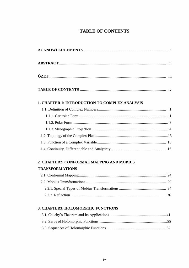
TABLE OF CONTENTS
ACKNOWLEDGEMENTS ....................................................................................... …i
ABSTRACT ................................................................................................................ ...ii
ÖZET ........................................................................................................................... ..iii
TABLE OF CONTENTS .......................................................................................... ..iv
1. CHAPTER 1: INTRODUCTION TO COMPLEX ANALYSIS
1.1. Definition of Complex Numbers ....................................................................... .. 1
1.1.1. Cartesian Form ........................................................................................... ...1
1.1.2. Polar Form .................................................................................................... .3
1.1.3. Streographic Projection ................................................................................ .4
1.2. Topology of the Complex Plane...........................................................................13
1.3. Function of a Complex Variable ........................................................................ .15
1.4. Continuity, Differentiable and Analyticty .......................................................... .16
2. CHAPTER2: CONFORMAL MAPPING AND MOBIUS
TRANSFORMATIONS
2.1. Conformal Mapping ........................................................................................... .24
2.2. Mobius Transformations .................................................................................... .29
2.2.1. Special Types of Mobius Transformations ................................................. .34
2.2.2. Reflection......................................................................................................36
3. CHAPTER3: HOLOMORPHIC FUNCTIONS
3.1. Cauchy’s Theorem and Its Applications .......................................................... 41
3.2. Zeros of Holomorphic Functions .......................................................................55
3.3. Sequences of Holomorphic Functions............................................................... 62

v
4. CHAPTER4: RIEMANN MAPPING THEOREM..............................................66
5. CHAPTER 5: CONCLUSION...............................................................................75
REFERENCES............................................................................................................76

i
ACKNOWLEDGEMENTS
First of all, I feel very responsible to thank my supervisor Prof.Dr. Kaya I. OZKIN for
working hard with me.
Also, I would like to thank Assoc.Prof.Dr Evren HINCAL, Assist.Prof.Dr. Abdurrahman
Mousa OTHMAN, Assist.Prof.Dr. Burak SEKEROGLU, for guiding me while I was writing
my dissertation. I appreciate Assoc.Prof.Dr. Harun KARSLI for helping me organise my
dissertation.
I shouldn’t forget to thank my mother, Cemile GULFIDAN, my father Halil GULFIDAN, and
my brother Ömer GULFIDAN for supporting me from their heart.
I am very thankful to my best friend Selen VAIZ for encouraging me in this hard journay. I
also appreciate Meral İpek AZIMLI for spending effort for me and believing me from her
heart.

ii
ABSTRACT
Eventhough, real differential functions are one of the main subject of real analysis, they are
also take place in the centre of complex functions theorem.
Functions which are both holomorphic and bijective, are called biholomorphic functions. If
two spaces have biholomorphism between them, then these two spaces are biholomorphically
equivalent.
Biholomorphically equivalence is very important in complex analysis, because instead of
working on complicated spaces, we can work on simpler work on known spaces.
For example, suppose and are both open subsets of If and mapping is
biholomorphic, then must be holomorphic in order to make function
holomorphic.
Basically, in comlpex functions theorem, spaces which are holomorphically equivalence are
identical.
Riemann Mapping Theorem is a big result for sufficient of conditions of biholomorphic
equivalence in complex function theory. Riemann Mapping Theorem provides an easy way
for building biholomorphically equivalence. It quarantees the presence of biholomorphic
functions and it also shows that, building biholomorphic transformations between spaces is
unnecessary.
Keywords: Biholomorphically equivalent, Open Mapping Theorem, Montel’s Theorem,
Hurwitz’s Theorem, Mobius Transformations, Conformal Mapping, Riemann Mapping
Theorem.

iii
ÖZET
Her nekadar reel diferensiyellenebilir fonksiyonlar reel analizin temel konularından biri ise
de, holomorfik fonksiyonlar, karmaşık fonksiyonlar teorisinin merkezinde yer alırlar. Burada
holomorfik ve birebir ve üzerine olan fonksiyonlara biholomorfik fonksiyonlar denilecektir.
Aralarında biholomorfizm olan iki uzay biholomorfik eşdeğerdirler.
Karmasık analizde biholomorfik eşdeğerlilik önemlidir. Çünkü bu sayede yapısı hayli karısık
olan bir uzayla calısmak yerine, yapısı daha yakından bilinen bir uzayı alarak calısmak
mümkün olabilmektedir. Örneğin, U ve V, C nin açık alt kümeleri oldugunu varsayalım.
Eger f : U → V donüsümü biholomorfik ise bu durumda herhangi bir g : U → fonksiyonun
holomorfik olması icin gerek ve yeter kosul, go f : U → bileske foksiyonunun holomorfik
olmasıdır .
Temelde karmaşık fonksiyonlar teorisinde holomorfik olarak eşdeğer uzaylar aslında özdeştir-
ler.
Karmaşık fonksiyonlar teorisinde Riemann dönüşüm teoremi, biholomorfik eşdeğerlik için
hangi koşulların yeterli olacağını belirtmesi bakımından çok önemli büyük bir sonuçtur.
Uzaylar arasında biholomorfik dönüşümler inşaa etmek genellikle zordur.
Riemann dönüşüm teoreminin sagladığı kolaylık belirli tipten uzaylar arasında biholomorfik
fonksiyonun varlığını garanti etmesi ile artık uzaylar arasında biholomorfik dönüşümler insaa
etmenin gereksiz olacağıdır.
Anahtar Sözcükler: Biholomirfik Eşdeğerlik, Açık Dönüşüm Teorisi, Montel Teorisi,
Hurwitz’s Teorisi, Mobyüs Dönüşümleri, Konform Dönüşümler, Riemann Dönüşüm Teorisi.

1
CHAPTER 1
INTRODUCTION TO COMPLEX NUMBERS
The goal of this chapter is to understand complex numbers, complex functions and their
properties. The chapter is written in order to explain the main topic of my dissertation. The
difference between complex functions and real functions are mentioned and suitable
examples are given. Later on this chapter, topologic properties of complex planes are
discussed. The most importantly, we will see derivatives of complex functions and we will
also talk about what are the conditions on these subjects.
1.1 Definition of Complex Numbers
We can represented complex number in cartesian form, polar form and spherical form.
1.1.1 Cartesian form
Let
*( ) +
We call the set of all complex numbers. This means that ( ) is complex
number, where and , and x is called the real part of the given complex number,
which is
and similarly y is called the imaginary part of the given complex number, which is
Addition to these is called conjugate of , which is,
and the modulus of a complex number z , that is
| | √

2
and also this is positive real number.
We will talk about some basic properties of complex numbers in cartesian form. Assume that
which are, where all components
of all z are in
If then we have
If and
For where and then
The conjugate of is equal to . That is
| |
From assertion, we have and clearly .
( ) ( )
(1.1)
We know that
| | √
(1.2)
If we take square 1.2 side by side, then we have
| |
(1.3)
We can see that 1.1 and 1.3 are equal. Finally, we have

3
| |
| | | | | | | |
| | | |
| | | | | |
| | | | | |. This is called triangle inequality.
Since
| |
( )
( )
|
|
| |
| | where | |
1.1.2 Polar form
Suppose that | |and is argument of any complex number , then,
and ( ) is called polar form of z.
Clearly, | | √ .
/ Argz is called principle argument,
where Then
For example, let and we have | | √ √ and also
√ .
/
is polar form of
Now, we talk about some basic properties of complex numbers in polar form. Let
( ) ( )

4
( ( ) ( )
( ( ) ( ))
( )
.
/
Example 1.1 Find Argz and arg z where √
Solution. We have z lies in fourth quadrant of complex plane. The modulus of z is
| | √
Since z lies in fourth part in , the principal argument of z is equal to
We know
that, . And finally we have,
1.1.3 Stereographic Projection
Let ( ) is any point in Through the points N and Z we draw the straight line NZ
intersecting the sphere S at a point ( ). Then is called the stereographic
projection. Consider the unit sphere S in , that is
*( )
+
Equation of the line M passing through Z and N

5
{( ) (( ) ( ) ) }
( )
( )
( ) ( )
*( ) ( ) ) +
Then we must have
( ) ( )
( ) ( )
( ) | |
| | (| | )
| |
| | (1.4)
We have
( ) (1.5)
If we put 1.4 in 1.5 then we have
0 | |
| | 1
*| | | |
| | +
| |
| | ( )
Similarly, we have
( ) (1.7)
If we put 1.4 in 1.7, we have,

6
| |
| | ( )
And so we have clearly
| |
| | ( )
From 1.6, 1.8, and 1.9 we have
( ) (
| |
| | | |
| | )
Example 1.2 Write the given complex number
in three form of complex numbers.
Solution. Now, we multiply numerator and denumerator of the given number with then
we have
This is the cartesian form of the given z. Now, we compute and r, which are;
| | √(
) (
)
√
and
(
)
Therefore
√
(
)
this is polar form of the given z. And finally,

7
| |
(√ )
| |
(√ )
| |
| |
Therefore (
) is the spherical form of the given z.
Definition 1.3 * + is called the extended complex plane.
In general if for , ( ) on then
| |
| |
Under stereographic projection, we have
| |
| |
| |
Now we assume that ( ) is a sequences of S which converge ( ) and let * + be
the corresponding sequence of points in . Now, we show that if | | then
( ) ( ).
Let

8
| |
| |
|
|
| |
If | | we have
|
|
| |
|
|
| |
| |
| |
| |
.
Now, if we show ( ) , then we say that is a continuous function.
( ) (
| |
| | | |
| |
at | | we have
| |
| |
| |
| |
| | (
| | )
| | (
| | )
Hence ( ) which show that is a continuous function. Now we can define a function
. We can see that is one-to-one and onto. Hence has inverse function, which is
. We know that ( ) ( ) . If we put in
and we have
( ) and ( )
9
and
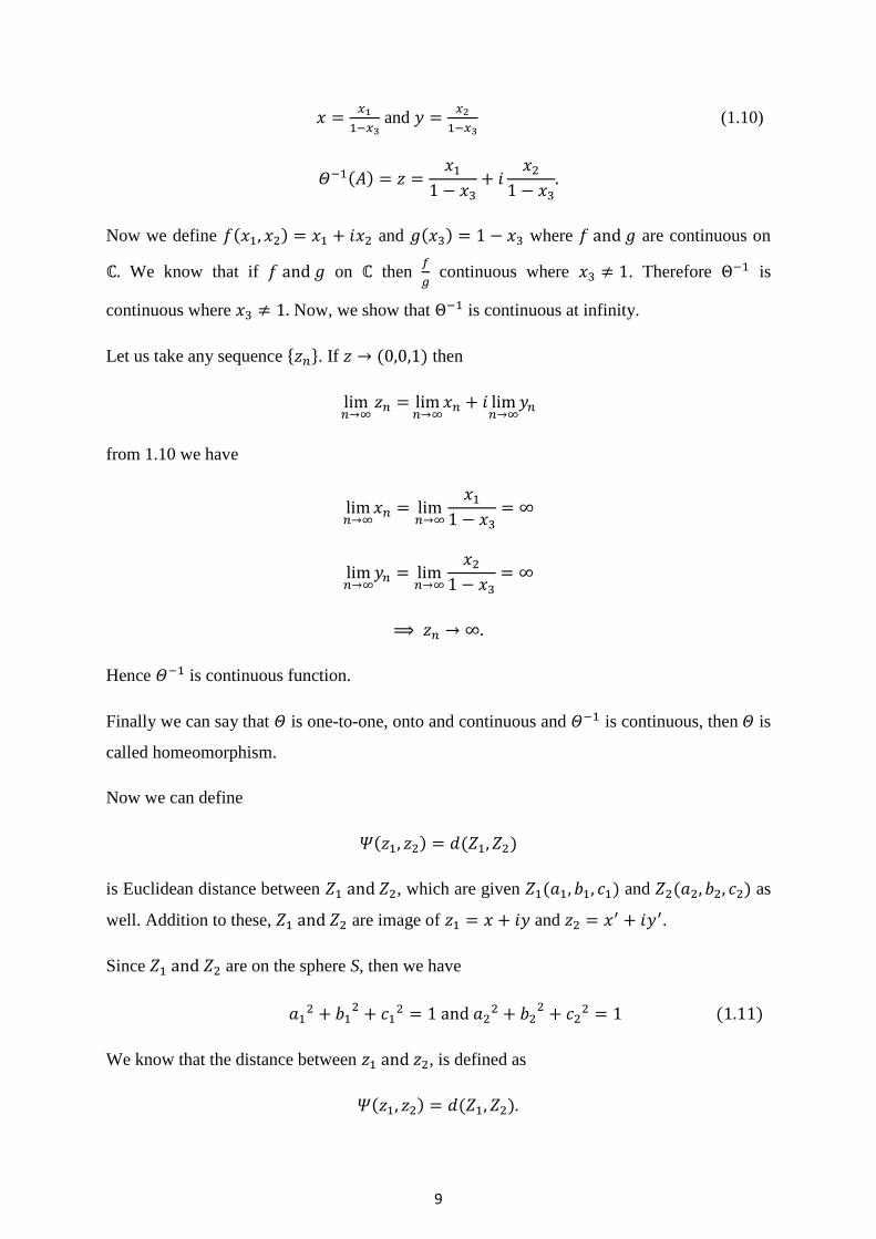
(1.10)
( )
Now we define ( ) and ( ) where are continuous on
We know that if on then
continuous where . Therefore is
continuous where Now, we show that is continuous at infinity.
Let us take any sequence * +. If ( ) then
from 1.10 we have
Hence is continuous function.
Finally we can say that is one-to-one, onto and continuous and is continuous, then is
called homeomorphism.
Now we can define
( ) ( )
is Euclidean distance between , which are given ( ) and ( ) as
well. Addition to these, are image of and .
Since are on the sphere S, then we have
( )
We know that the distance between , is defined as
( ) ( ).

10
Hence we have
( ) √( ) ( ) ( )
√
from 1.11 we have
( ) √ ( )
√ √ (1.12)
since are on S, clearly we have
| |
| |
| |
| |
| |
| |
| |
| | ( )
If we put 1.13 in 1.12, we have
( ) | |
√| | | |
If is the point at infinity then
( )
| |
√| | | |
| |
| | |
| | |
√| | | | √
| |
| |
| |
| |
We have some important theorems about stereographic projection.

11
Theorem 1.4 Streographic projection take circle to circle and lines.
Proof. We assume that K is a circle on Riemann sphere.
*( )
+
If K passes through ( ) then we have
from definition of stereographic projection we have
| |
| | | |
| | ( )
If we put 1.14 in
then we have
( )
( ) ( )
( )( ) ( )
If , then 1.15 becomes
which is equation of a line. If then 1.15 is
( )( )
is the equation of a circle. □

12
Theorem 1.5 Let . Then the corresponding image of K on S is
a is a circle in S not containing ( ) if K is circle
a line in S containing ( ) if K is a line.
Proof. Now, we consider the general equation of a circle in .
*( ) ( ) + ( )
Now we put 1.10 in 1.16 then we have,
*
( )
( ) +
(
)
( )
( ) ( )
Let . Clearly, from 1.16 we have
this is equation of the line. Since from 1.17
( )
this equation containing ( ). If K is a line then ( ) . Now we assume that
and Then from 1.16 we have
( )
this is equation of circle and
( )
we can see 1.18 not containing ( ) □
13
1.2 Topology of the Complex Plane
In this section we will talk about the topology of the complex plane and we will see
difference between them.
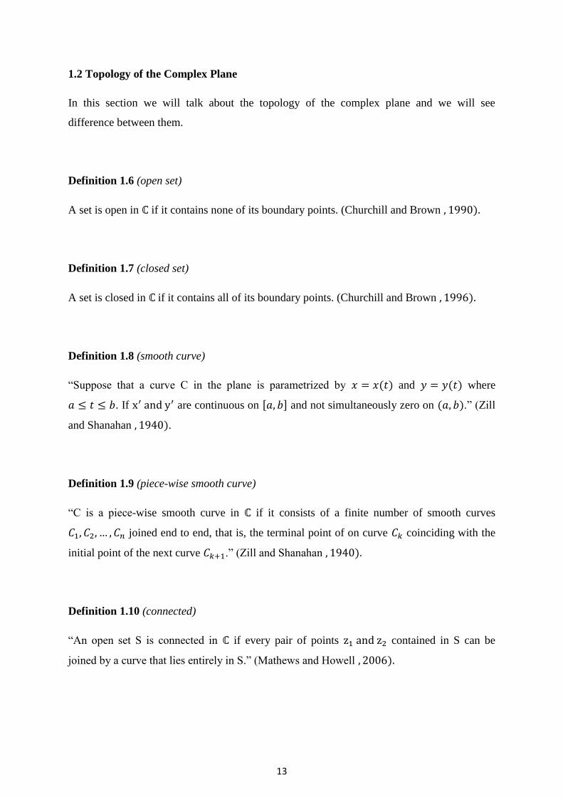
Definition 1.6 (open set)
A set is open in if it contains none of its boundary points. (Churchill and Brown )
Definition 1.7 (closed set)
A set is closed in if it contains all of its boundary points. (Churchill and Brown )
Definition 1.8 (smooth curve)
“Suppose that a curve C in the plane is parametrized by ( ) and ( ) where
. If are continuous on , - and not simultaneously zero on ( ).” (Zill
and Shanahan ).
Definition 1.9 (piece-wise smooth curve)
“C is a piece-wise smooth curve in if it consists of a finite number of smooth curves
joined end to end, that is, the terminal point of on curve coinciding with the
initial point of the next curve .” (Zill and Shanahan )
Definition 1.10 (connected)
“An open set S is connected in if every pair of points contained in S can be
joined by a curve that lies entirely in S.” (Mathews and Howell )

14
Definition 1.11 (simply connected and multiply connected)
“A domain D in is simply connected if its complement with respect to . A domain that is
not simply connected is called multiply connected domain, that is, it has ” in it.” (Zill
and Shanahan )
Definition 1.12 (domain)
“A domain is a nonempty open connected set in ” (Ponnusamy )
Definition 1.13 (region)
“A domain together with some, none or all of its boundary points is reffered to as a region in
” (Ponnusamy )
Definition 1.14 (bounded and unbounded)
“A set S is bounded in if | | whenever else it is
unbounded.” (Stein and Shakarchi )
Definition 1.15 (compact set)
“ If a set S is closed and bounded then it is called compact in ” (Zill and Shanahan )

15
1.3 Function of a Complex Variable
Definition 1.16 (complex function)
Let A and B be two nonempty subset of . A function from A to B is a rule, , which assigns
each a unique element . The number is called the
values of at and we write ( ). If z varies in A then ( ) varies in B. We
also write , ( ). We have two real-valued functions , ,
then by defining ( ) ( ) ( ), ( ) We obtain , where A is
subset of .
“ In this section introduction, we defined a real-valued function of a real variable to be a
function whose whose domain and range are subsets of the set of real numbers. Because
is a subset of the set of the complex numbers, every real-valued function of a real variable
is also a complex function. We will soon see that real-valued functions of two real variables x
and y are also special types of complex analysis. This functions will play an important role in
the study of complex numbers.” (Zill and Shanahan , - )
If ( ) is a complex function, then the image of under is .
For example; let and is complex function. Then the image of z under
( )
( ) and ( )
Where u is real part, v is imaginary part of the given complex function.
“A useful tol for the study of real functions in elementary calculus is the graph of the
function. Recall that if ( ) is a real-valued function of a real variable x, then the graph
of is defined to be the set of all points ( ( )) in the two-dimensional Cartesian plane. An
analogous definition can be made for a complex function. However, if ( ) is a
complex function, the both z and w lie in complex plane. It follows that the set of all points
( ( )) lies in four-dimensional space. Ofcourse, a subset of four-dimensional space cannot
be easily illustrated. Therefore; we cannot draw the graph a complex function.” (Zill and
Shanahan, )

16
Consider the real function ( ) . We can draw the given real function in Cartesian
plane. But if ( ) is a complex function then the image of ,
we have
( ) ( )
where , is the line in w-plane. Finally we have in z-plane
mapped onto in w-plane under . Since , this is mapped onto
, under .
1.4 Continuity, Differentiable and Analyticity
Definition 1.17 (continuity)
“ Let be an open set and let be a function. We say is continuous at
if and only if
( ) ( )
and that is continuous on A if is continuous at each point in A.” (Marsen and
Hoffman )
Definition 1.18 (differentiability)
“ A complex valued function ( ) is differentiable at if
( ) ( )
( ) ( )
exists. The function is said to be differentiable on D if it is differentiable at every points of
D.” (Gamelin ).
Definition 1.19 (analyticity)
“ Let D be an open set in and is a complex valued function on D. The function is
analytic or holomorphic at the point if
( ) ( )

17
converge to a limit. The function is said to be holomorphic or analytic on D if is
holomorphic or analytic at every point of D.” (Stein and Shakarchi )
Definition 1.20 (Cauchy-Riemann equations)
Properties of real and imaginary parts of the differentiable function ( ) ( )
( ) will be deduced by specializing the mode of approach. Firstly, we assume that h
approaches to zero along the real axis
( ) ( )
( ) ( ) ( ) ( )
( ) ( )
( ) ( )
Since is differentiable at , then
( ) ( )
( ) ( )
must be exists. And also we know that
( ) ( )
and
( ) ( )
Thus we have
( )
( ) ( )
( )
Now we assume that h approach 0 along the imaginary axis. Then for , is real we
have
( ) ( )
( ) ( )
( ) ( )
( ) ( )
( ) ( )
( ) ( )

18
(
)
( )
Example 1.21 Show that the given complex function ( ) satisfies Cauchy Riemann
equations.
Solution.
( ) ( )
( ) ( )
satisfies all Cauchy-Riemann equations.
Note that since we talked about complex functions in cartesian form and polar form, now we
will talk in terms of . We know that, gives that
If we write complex function
( ) (
) (
)
Also we can write
[
]
[( ) ( )]
and is equivalent to the system
Thus we have following theorem.

19
Theorem 1.22 “A necessary condition for a function to be differentiable at a point a is that
satisfies the equation at a.” (Ponnusamy )
Now, we will see, we can write CR-equations in polar form. Let be differentiable at a point
z. Since we can write any complex function in polar form, we have
( ) ( ) ( )
and also . (1.22)
We have from Chain rule;
( )
Now in 1.22 we take the derivatives x and y with respect to r and put in 1.23 and we have
( )
Similarly, we have from Chain rule;
( )
Now in 1.22 we take derivative x and y with respect to and put in 1.25 and we have;
( )
( ) ( )
Similarly, again we have from chain rule;
( )
Now, we already have derivative of x and y with respect to . We can put in 1.27 and we
have;
( )
Finally we have

20
( )
Now we already have derivative of x and y with respect to We can put in 1.29
( )
( ) ( )
Now, we know that CR-equations in cartesian form, that is,
(1.31)
If we put 1.31 in 1.24, 1.26, 1.28 and 1.30 we have,
(
( )
( )) (
( )
( ))
( )
(
( )
( )) (
( )
( ))
( )
and in 1.32 and 1.33 are called CR-equations in polar form.
Example 1.23 Show that the given complex function ( ) satisfies
Cauchy-Riemann equations in polar coordinates.
Solution.
( ) ( )
satisfies Cauchy-Riemann equations in polar coordinates.
CR-equations are necessary but not sufficient for derivative of a complex function. If any
complex function differentiable then must be satisfy CR-equations but it is conversely not
true. We have following useful example.

21
Example 1.24 Determine ( ) ,
- is differentiable or not at
Solution. We can see that ( ) at .
satisfies CR-equations but on the line ( )
( )
( ) ( )
doesn’t exists. Hence is not differentiable at
Theorem 1.25 “ Let ( ) ( ) ( ) be defined in a domain D, and let
have continuous partial derivatives that satisfy the Cauchy Riemann equations
for all points in D. Then ( ) is analytic in a domain D.”
(Ponnusamy )
Definition 1.26 (singular point)
“ If a function fails to be analytic at a point but is analytic at some point in every
neighborhood of , then is called a singular point of ” (Churchill and Brown )
Definition 1.27 (residue)
“ If a complex function has an isolated singularity at a point , then f has a Laurent series
representation
( ) ∑ ( )
∑ ( ) ∑ ( )
which converges for all z near . More precisely, the representation is valid in some deleted
neighborhood of or punctured open disk | | . The coefficient of
in

22
the Laurent series given above is called the residue of the function.” (Zill and
Shanahan )
Definition 1.28 (discrete or isolated)
“ A singular point is said to be isolated if , in addition, there is a deleted neighborhood
| | of throughout which is analytic.” (Churchill and Brown )
Definition 1.29 (Taylor expansion)
“ Let is analytic function throughout an open disc | |< centered at and with
radius , then at each point z in that disc, ( ) has a series representatiton
( ) ∑ ( ) ( )
is called a Taylor expansion of .” (Churchill and Brown )
Definition 1.30 (zero and pole of holomorphic function)
“ Let is analytic in an open domain D. If for ( ) then z is called zero of
holomorphic function . We say that is a pole of and the smallest such that
( ) ( )
is bounded near is called the order of the pole at ( )
Definition 1.31 (meromorphic function)
“ A function is said to be meromorphic in a domain D if it is analytic throughout D except
for poles.” (Churchill and Brown )

23
Definition 1.32 (sequences and subsequences)
A mapping is called a sequence. Suppose * + is a sequence of points in
and that * + is a strictly increasing sequence of natural numbers Then the sequence { } is
called a subsequence of * +
Definition 1.33 (converge uniformly)
Consider an open set and a sequence of functions { } converge uniformly to if
| ( ) ( )| . Note that this
must work for all , it depends only on .
Definition 1.34 (converge normally)
We say that { } converge normally to if for each compact and there exist
such that | ( ) ( )| .

24
CHAPTER 2
CONFORMAL MAPPING AND MOBIUS TRANSFORMATIONS
The goal of this chapter is, given some basic definition, theorem and properties about
conformal mapping and Mobius transformations. We are going to see how the last chapter is
important.
2.1 Conformal Mapping
Definition 2.1 (homeomorphism)
A function is a homeomorphism if is a bijection and if both are
continuous.
Definition 2.2 (automorphism)
The set of all conformal bijections are defined by .
Theorem 2.3 If f is an analytic function in a domain D containing , and if , then
is a conformal mapping at
Proof. Assume that is analytic function in a domain D containing and . Let
be two smooth curves in D and parametrized by and parametrized by
, respectively, with . Let maps the curves
onto the curves . Let is angle between and is angle between image
of , respectively, . Now we have to show that . are
parametrized by ( ) ( ). Now, we compute the tangent

25
vectors
to at ( ) ( ). We can use the chain
rule;
( )
( )
We have already are smooth and both and
are nonzero. By hypothesis we
have . Hence,
( ) ( )
Therefore we completed this proof. □
Example 2.4 Find all points where the mapping is conformal.
Solution. Firstly we have . Now, if we take the first derivative of the given
function, we have,
is conformal mapping at z for all
Example 2.5 Determine where the complex mapping
is conformal.
Solution. Firstly we have
. Now we take the first derivative of the given
function with respect to z, we have,

26
Now, we have three roots of z, that is,
Then we have,
√
√
is conformal mapping at z for all
√
√
.
Example 2.6 Find the image
{ }
under

27
Solution. Let we define
This means that
Let
since
.
Hence the image of H under is unit disc.

28
Example 2.7 Find the image of
{ | | }
under
Solution. Let we define
This means that
Since | | we have
|
|
| | | |
| | | |
.
Let Since , we have

29
Hence, the image of K under is first quadrant of plane.
2.2 Mobius Transformations
In this section we will talk about mobius transformations and their basic properties. Mobius
transformations are very important because this transformations are basic of conformal
mapping.
Definition 2.8 Let and then
and
is called Mobius transformation.
2.1 is called automorphism and 2.2 is called anti-automorphism. We will discuss some basic
properties about automorphism and anti-automorphism of .
Every T anti-automorphism, it can be define composition of automorphism and
complex conjugate transformation of
The composition of two anti-automorphisms is automorphism.
A composition of an automorphism and an anti-automorphism again anti-
automorphism.

30
The automorphism keep constant of the magnitude of angles but inverse the direction.
Now, in this part when we investigate mobius transformations, we will consider mobius
transformation in form 2.1.
is called determinant of mobius transformation T. We must take
because in definition of mobius transformation gives us
If then we take . This means that T will be constant function. In
the same time if then T is one-to-one function. Mobius transformation
independent to coefficient If { } then, gives us
in this manner again to get T. Therefore, we multiply numerator and denumerator of 2.1 with
√
Then we have
√
√
√
√
the determinant of 2.4 is
(
√
√ ) (
√
√ )
Consequently, we can take instead of , .
Definition 2.9 Let
, then
and (
)
If

31
Theorem 2.10 Every mobius transformation from to are one-to-one and onto.
For identity transformation then we can write
Hence identity transformation is any mobius transformation. Addition to these the
inverse mobius transformation of T is
and clearly we can say that transformation is also mobius transformation. Therefore we
can give the following theorem.
Theorem 2.11 The set
{
}
is a group with respect to composition.
Definition 2.12 (similarity transformation)
is called similarity transformation.
Let { } is the set of similarity transformations.
Since then . Addition to this we can write
Then
Specially H is closed with respect to composition. Then

32
Definition 2.13 (general linear group)
(
)
is called General Linear Group and we can show in
form .
Now, we can define relation between Mobius transformation and matrices
(
)
Theorem 2.14 is a homeomorphism. Seperately since is
onto, is called epimorphism and its kernel defined as
{ }
{(
)
}
{(
) }
={(
) }
If we take then
{(
) }
{ (
) }
{ }.
This is proof of the following theorem.

33
Theorem 2.15 Let I is an identity matrix in form 2x2. Then kernel of homeomorphism ,
{ }
two matricesdefined as the same mobius transformation in if and only if
that is to say for
A necessary of first isomorphism theorem, for transformation then
{ }
is called Projective General Linear Group and we can define this .
Because of this, it can be . For every since
then
{ }
is called homeomorphism.
{ (
) }
the kernel set of function of determinant is called special linear group. Because of
determinant is onto, necessary of first isomorphism theorem, we have
If then and for Since it can be
show this for every mobius transformation in write in form
Additionally, under in . This is proof of following theorem.
Theorem 2.16

34
2.2.1 Special types of mobius transformations
Definition 2.17 (translation)
is called translation.The transformation translation keeps constant of
infinity and it makes a movement on plane.
Definition 2.18 (rotation)
is called rotation. If then rotation is counterclockwise, if
then rotation is clockwise, The transformation rotation makes 0 and infinity constant.
Definition 2.19 (inversion)
is called inversion.
Definition 2.20 (magnification)
is called magnification.
The transformation magnification makes 0 and infinity constant. The transformation
magnification affects as similarity on plane and longtitude is expanded or shrinked by the r
multiplier.
Theorem 2.21 Every mobius transformation can write composition of translation,
magnification, rotation and inversion.
Proof. Every mobius transformation knows in form

35
If then
. Let
and
Then
therefore, we have
This transformation makes infinity constant. If then we can use so we
can write
Because of there we can write
(
) □
Definition 2.22 (Euclidean circle)
The set of points in satisfy | | are called Euclidean circle.
The set of points in satisfies | | | | are called Euclidean line. Euclidean
circle or { } are called circle in . In there is any Euclidean line.
Theorem 2.23 If a circle in then the image of C under mobius transformation T, is
a circle in
Proof. We know that general equation of circle is
.
the transformation in form
We have to show that is a circle.

36
since
, clearly we have
If we put in general equation of a circle, we have
(
) (
) (
) (
)
Clearly we have
[ ] [ ]
[ ] [ ]
In this section the coefficient of is real. Because and are real. Similarly the
coefficient of and are real. Because of there, image of circle under again circle.
2.2.2 Reflection
Let C is a circle in , which is
If then C is an Euclidean circle in .

37
Let the center of C is w and radius is r. { } on the line which include w and z,
such that
| | | |
are on the same line. There, is called reflection of z with respect to C.
Definition 2.24 (reflection transformation)
Let w is a center and r is radius of C. is called reflection transformation.
From this definition we can see the point z goes to infinity, when w approaches to .
Similarly, when w approaches to z, goes to infinity. Therefore, we define
and . And is continuous and magnificate to any transformation in
in the same time. Seperately,
If . In other words, reflection of any points on C is itself. If ,
then
| | | | | |
Since and ( on the same line
then
therefore

38
Theorem 2.25 If are reflect points with respect to C then the image of
under
, which are are reflect points with respect to C.

39
CHAPTER 3
HOLOMORPHIC FUNCTIONS
This chapter is dedicated to give some definition, lemma and some theorems about
holomorphic functions, Fundamental Theorem for Contour Integral, Cauchy’s Integral
Theorem and its applications, such as Cauchy’s Theorem or Cauchy-Goursat Theorem,
Bounding Theorem, Taylor’s Theorem, Cauchy’s Integral Formula, Cauchy’s Integral
Formula for Derivatives, Cauchy’s Inequality, Cauchy Residue Theorem, Argument Principle
Theorem, Rouche’s Theorem, Open Mapping Theorem, Maximum Modulus Theorem,
Maximum Modulus Principle, Montel’s Theorem and Hurwitz’s Theorem, as well.
Definition 3.1 (antibiholomorphic)
If the analytic function preserve angle but not preserve its orientation then this function is
called antibiholomorphic.
Example 3.2 We have ( ) . We assume that the angle has
positive orientation. For conjugate of ( ) . And its angle is – . Also we can
say, preserve magnitude of angle but not preserve is orientation. Then is
antibiholomorphic function.
Now, we are going to start useful lemma about holomorphic functions.
Lemma 3.3 Suppose that is simply connected and open that is holomorphic
and nowhere vanishing. Then there exists a holomorphic function * + such that
, ( )- ( )

40
Proof. Let is simply connected and open subset of Since is nonvanishing, we can say
that ( )
( ) is also holomorphic. Then there exists a holomorphic function such that
( ) , ( )- (3.1)
ıf we take derivative 3.1 with respect to z then we have
( ) ( )
( ) ( )
Since ( )
( ) holomorphic, then ( ) must be holomorphic, as well. Now we choose . If
we put in 3.1, we have
( ) , ( )-
Clearly, we have
( ) ( ) ( )
Now, , from 3.2
[ ( ) ( )] ( ) ( ) ( ) ( ) ( )
( ) ( ) ( ) ( )
( ) ( )
( ), ( ) ( )-
( ) ( ) is constant. Now, from 3.3 we have
( ) ( )
Hence we have
( ) ( )
Finally, we have
( ) ( ) ( )
41
If we take square of 3.4
, ( )- [ ( ) ]
( ) ( )
□
3.1 Cauchy’s Theorem and Its Applications
Most of powerful theorems proved in this section. Importance of Cauchy’s Theorem lies in
its applications. Addition to these, there is a such a good relationship between the different
theorems.
First we will talk about some famous theorem which are Fundamental Theorem of Contour
Integral and Green’s Theorem. Because consequence of these theorems are very useful for
Cauchy Integral Theorem and its applications.
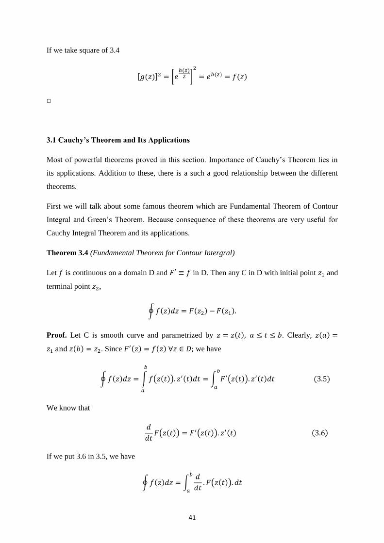
Theorem 3.4 (Fundamental Theorem for Contour Intergral)
Let is continuous on a domain D and in D. Then any C in D with initial point and
terminal point ,
∮ ( ) ( ) ( )
Proof. Let C is smooth curve and parametrized by ( ) . Clearly, ( )
( ) . Since ( ) ( ) we have
∮ ( ) ∫ ( ( )) ( ) ∫ ( ( )) ( )
( )
We know that
( ( )) ( ( )) ( ) ( )
If we put 3.6 in 3.5, we have
∮ ( ) ∫
( ( ))

42
( ( )) ( ( ))
( ) ( )
Theorem 3.5 (Cauchy Integral Theorem of Cauchy-Goursat Theorem)
Suppose that a function is analytic in a simply connected domain D and is continuous in
D. Then in D such that
∮ ( )
Proof. Let ( ) ( ) ( ). Since is analytic, ( ) satisfies Cauchy Riemann
equations, that is,
( )
And also we can write . Hence clearly we have
∮ ( ) ∮( ) ( )
∮( ) ∮( )
From Green’s theorem we have
∮( ) ∬( )
and
∮( ) ∬( )
This means that
∮ ( ) ∬( ) ∬( ) ( )
If we put 3.7 in 3.8 then we have

43
∮ ( ) ∬( ) ∬( )
∮ ( )
Example 3.6 Use 3.5 and evaluate
∮
where | | .
Solution. We have two singular points, which are and And also they lie in C.
We can write again the given function in this form, that is,
( )
( )
.
Now, we have
∮
∮
∮

44
Example 3.7 Use 3.5 and evaluate
∮
where | | .
Solution. We have two singular points, which are . And also they lie in
C. We can write again the given function in this form, that is,
( ) ( )
We have
∮
∮
∮
Remark 3.8 If in simple closed , then for we have
∮
( ) {
}
Now we will apply the given remark in this following example.

45
Example 3.9 Evaluate the given integral
∮ [
( ) ]
where | |
Solution. Firstly, we can separate the given integral
∮
∮
( )
We have zeros of the given functions are and . They are also inside | |
From remark, we have
Now, we will give some information about Bounding theorem. This is very useful for Cauchy
Integral formula.
Theorem 3.10 (Bounding Theorem or ML-Inequality)
If is continuous on a smooth curve C and if | ( )| on C then
|∮ ( ) |
where L is length of C.
Proof. From triangle inequality;
|∮ ( ) | |∑ ( )
| ∑| ( )| | |
∑| |
( )
where is distance between two points on C. It cannot be greater than length L of C.
Hence we have;
| | ( )
If we put 3.10 in 3.9 we have

46
|∮ ( ) |
□
Theorem 3.11 (Cauchy Integral Formula)
Let g is a holomorphic in a simply connected domain D and C is any simple closed contour in
D. Then
( )
∮
( )
Proof. Suppose that D be a simply connected domain, C is a simple closed contour and a
interior point of C. Addition to these, let be a circle at a, lies in C. We can write
∫ ( )
∫ ( )
From 3.5, we have
∫ ( )
∫ ( )
∫ ( ) ( ) ( )
( )∮
∮
( ) ( )
( )
Again from 3.5, we have
∮
( )
If we put 3.12 in 3.11, we have
∮
( ) ∫
( ) ( )
( )

47
Since g is continuous, we have there exists such that | ( ) ( )|
whenever | | Now, if we choose for | |
then from Bounding theorem;
we have
|∫ ( ) ( )
|
( )
This happens only bif the integral is 0. Thus
∮ ( )
( ) ( )
Finallyi if we divided 3.15 side by side by then we have
∮
( )
( )
□
Example 3.12 Evaluate
∮
where | |
Solution.
are zeros of the given function. Now, we can see inside of C.
Hence from Cauchy Integral formula we have;
∮
∮
( ) ( ) ∮
We can choose ( )
is analytic in C.
∮
( )

48
Theorem 3.13 (Cauchy’s Integral Formula for Derivatives)
Suppose that is analytic in a simply connected domain D and C is any simple closed
contour lying entirely within D. Then for in C,
( )
∮
( )
( )
Proof. Proof by induction. We already find for in 3.11. Now, we have to find for
Let C is ( ) And clearly we have ( ) for . We use 3.11
and write
( )
∮
( )
∫
( ( )) ( )
( )
Let we assume that
( ) ( ( )) ( )
( )
and derivative of ( ) equals to
( )
( ( )) ( )
( )
Now we have
( )
∫
( ( )) ( )
( ( ) )
For is true. Now, we assume that for is also true. And finally we have to show
that is true. If we continuous, we will see it is true. □
49
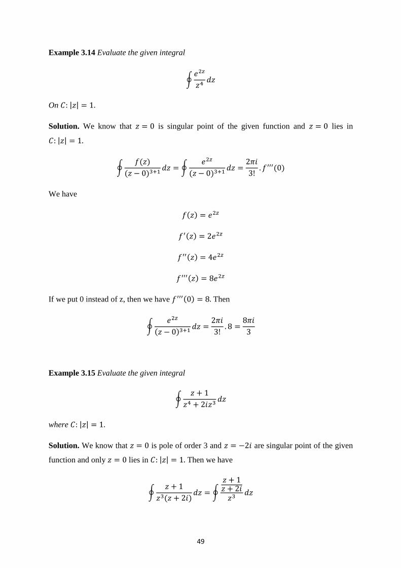
Example 3.14 Evaluate the given integral
∮
On | |
Solution. We know that is singular point of the given function and lies in
| |
∮ ( )
( ) ∮
( )
( )
We have
( )
( )
( )
( )
If we put 0 instead of z, then we have ( ) Then
∮
( )
Example 3.15 Evaluate the given integral
∮
where | |
Solution. We know that is pole of order 3 and are singular point of the given
function and only lies in | | Then we have
∮
( ) ∮

50
∮
( )
We have
( )
( )
( )
( )
( )
If we put 0 instead of z.
( )
then we have
∮
(
)
( )
Now we will talk about Taylor’s theorem. Because its application very useful for Cauchy’s
Inequality.
Theorem 3.16 (Taylor’s Theorem)
Let ( ) be analytic in a domain D whose boundary is C. If is a point in D, then ( ) may
be expressed as
( ) ∑ ( )
( )
and the series converges for | | where is distance from to the nearest point on
C.

51
Proof. Suppose that circle . From Cauchy Integral Formula
( )
∮
( )
( )
Let | |
| | | |
[
]
[
(
)
(
)
(
) (
)
]
( )
∮
( )
( )
∮
( )
( )
( )
∮
( )
( )
where
∮(
) ( )
But from 3.11 we have
( ) ( ) ( )( ) ( )
( ) ( )
Let | ( )| on . Then we have
∮ |
|
| ( )
| | |
.
/
∫| |
| |
| |
| | | |
( ).
/
∮| |
.
/
Since ,
52
.
/
Hence,
∑ ( )
( )
□
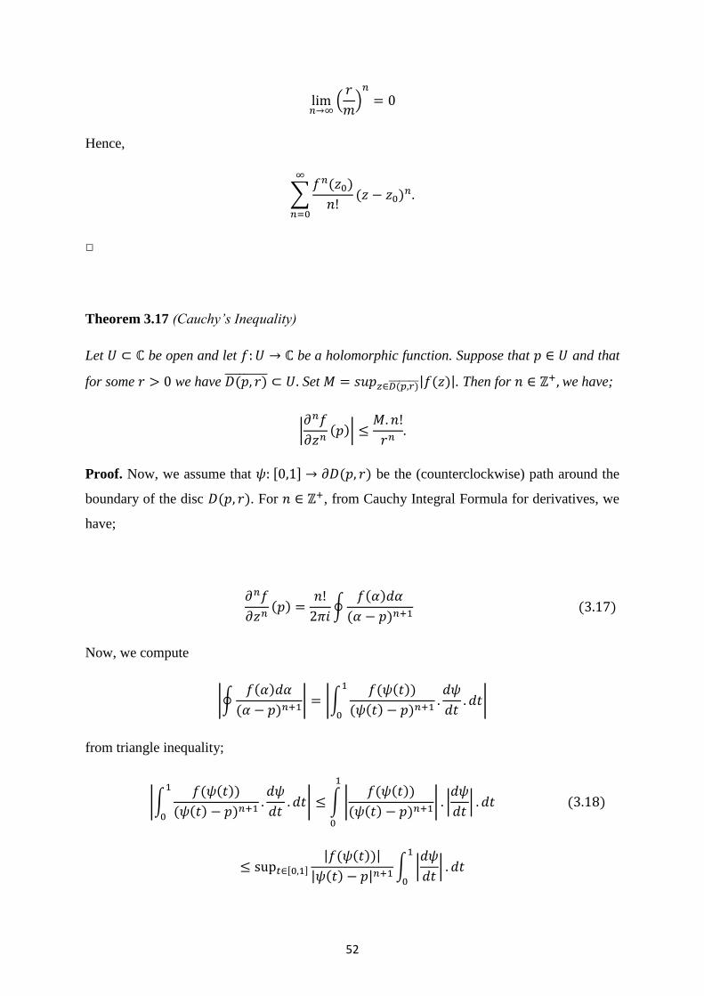
Theorem 3.17 (Cauchy’s Inequality)
Let be open and let be a holomorphic function. Suppose that and that
for some we have ( ) Set ( ) | ( )|. Then for we have;
|
( )|
Proof. Now, we assume that , - ( ) be the (counterclockwise) path around the
boundary of the disc ( ). For , from Cauchy Integral Formula for derivatives, we
have;
( )
∮
( )
( ) ( )
Now, we compute
|∮ ( )
( ) | |∫
( ( ))
( ( ) )
|
from triangle inequality;
|∫ ( ( ))
( ( ) )
| ∫ | ( ( ))
( ( ) ) | |
|
( )
, -
| ( ( ))|
| ( ) | ∫ |
|

53
The length of path is . If we put this length in 3.18, then we have
|∫ ( ( ))
( ( ) )
| , -
| ( ( ))|
| ( ) | ( )
Now, if we take the absolute of 3.17 then
|
( )| |
∮
( )
( ) |
, -| ( ( ))|
| | ( )
From assertion we know that
, -| ( ( ))| ( )
Finally, if we put 3.21 in 3.20, then we have
|
( )|
□
Theorem 3.18 (Cauchy Residue Theorem)
“Let C be a simple closed contour, described in the positive sense. If a function is analytic
inside and on C except for a finite number of singular points ( ) inside C,
then
∮ ( ) ∑ ( )
(Churchill and Brown, )
Example 3.19 Use 3.18 and evaluate the given integral
∮
( ) ( )
where | | .

54
Solution. We can see there only lies in | | We have
( ) ( )
( )
( ) (
)
( ) (
) [
(
)
]
⁄
( )
⁄
This means that
, ( ) -
Hence
∮ ( )
Example 3.20 Use 3.18 and evaluate the given integral
∮
where | |
Solution. Only lies in C. Then we have
( ) ( )
(
)

55
(
) [
( )
]
⁄
, ( ) -
∮ ( )
3.2 Zeros of Holomorphic Functions
In this section, we will demonstrate the zero of holomorphic functions which are not
identically zero are isolated.
Theorem 3.21 Let be connected and open set and let be a holomorphic. If
is not identically zero, then the zeros of are isolated.
Proof. Firstly, assume that is not identically zero. We have two cases:
Case 1: Let has no zeros. This is trivial solution.
Case 2: Suppose that has zeros. Let be a zeros of . Then
{ (
)
( ) }
From assertion we know that is holomorphic, and also Taylor’s theorem, we can say that
( ) ∑(
)
( ) ( )
( )
Similarly,
( ) ∑(
)
( ) ( )
( )
56
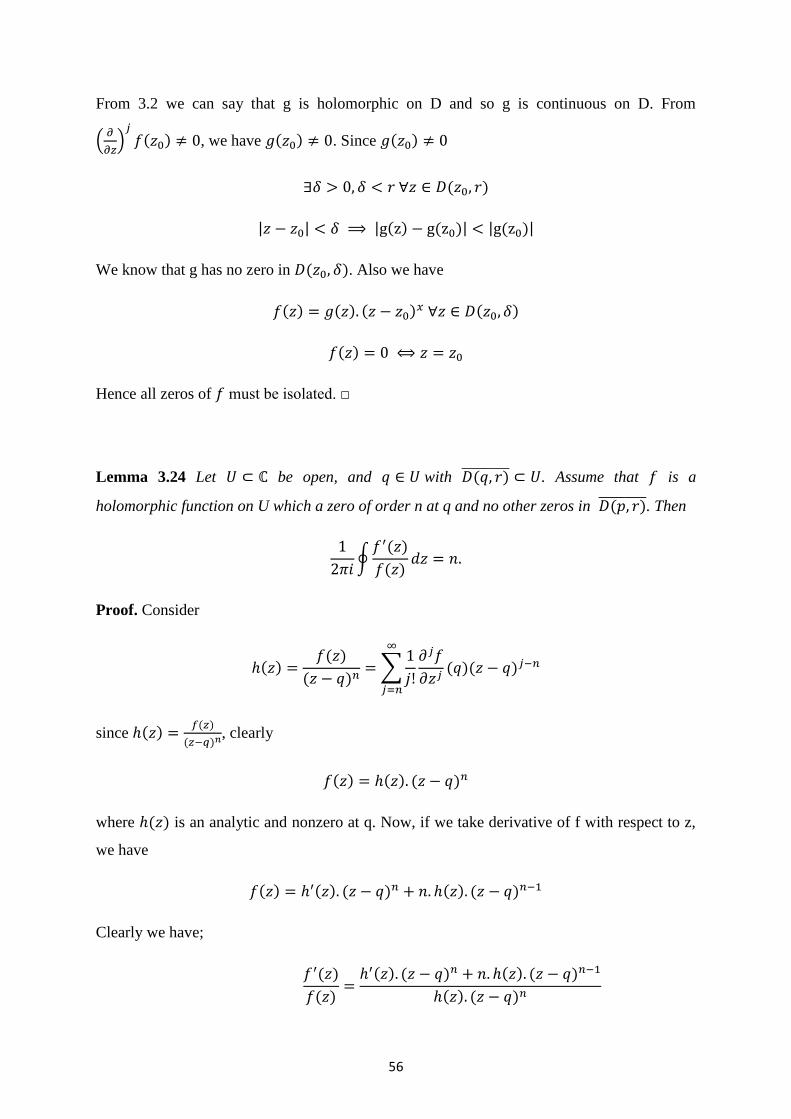
From 3.2 we can say that g is holomorphic on D and so g is continuous on D. From
.
/
( ) , we have ( ) . Since ( )
( )
| | | ( ) ( )| | ( )|
We know that g has no zero in ( ). Also we have
( ) ( ) ( ) ( )
( )
Hence all zeros of must be isolated. □
Lemma 3.24 Let be open, and with ( ) . Assume that is a
holomorphic function on U which a zero of order n at q and no other zeros in ( ) . Then
∮
( )
( )
Proof. Consider
( ) ( )
( ) ∑
( )( )
since ( ) ( )
( ) , clearly
( ) ( ) ( )
where ( ) is an analytic and nonzero at q. Now, if we take derivative of f with respect to z,
we have
( ) ( ) ( ) ( ) ( )
Clearly we have;
( )
( )
( ) ( ) ( ) ( )
( ) ( )

57
( )
( )
( )
( ) is holomorphic and nonzero on ( ) . By Cauchy Integral Theorem; we have
∮ ( )
( ) ∮
( )
( ) ∮
clearly,
∮
( )
( )
□
Theorem 3.25 (Argument Principle Theorem)
If is analytic and nonzero at point of a simple closed positively oriented contour C and is
meromorphic inside C, then
∮
( )
( ) ( ) ( )
where ( ) and ( ) are respectively, the number of zeros and poles of inside C.
Proof. Suppose is an analytic and nonzero function. Assume that
( ) ( )
( )
Since is an analytic, G is an also analytic and nonzero there. Consider inside C that is
zero of of order m. Then we know that can be written
( ) ( ) ( )
where ( ) is analytic and nonzero at . Now, if we take derivative of with respect to z,
we have,
( ) ( ) ( ) ( )
( )
From this, we have

58
( ) ( )
( )
( )
( ) ( ) ( )
( ) ( )
( )
( )
Since ( )
( ) is analytic at , this representation shows that G has a simple pole at with
residue equal to m. Now we have two cases:
Case 1: If f has a pole of order k at , then
( ) ( )
( ) ( )
where ( ) is analytic at and ( ) We already have
( ) ( )
( )
Take the derivative of 3.23 with respect to z
( ) ( ) ( )
( ) ( )
( ) ( )
If we put 3.24 in 3.23 we have,
( )
( ) ( ) ( ) ( )
( )
( )( )
( )
( )
Since ( )
( ) is analytic at , we find that G has a simple pole at with residue equal to
minus k. Finally by Residue theorem, the image of G around C must equal
∮ ( ) ∮ ( )
( ) [ ( ) ( )]

59
Case 2: If f has no poles inside C, then ( ) and we have
∮
( )
( ) ( )
where ( ) is the number of zero of f inside C. □
Now, we can say that our job will be easier because of Rouche’s Theorem. Now we will see
that applying to this theorem is very useful for Open Mapping Theorem.
Theorem 3.28 (Rouche’s Theorem)
Suppose ( ) and ( ) are analytic inside and on a simple closed contour C, with
| ( )| | ( )|
on C. Then ( ) ( ) has the same number of zeros as ( ) inside C.
Proof. Firstly we take the absolute value of ( ) ( ) We have
| ( ) ( )| | ( )| | ( )|
Since ( ) has no zero on C we can divide both side by | ( )|, then we have
| ( ) ( )|
| ( )| |
( )
( )|
for ( )
( ) cannot be equal to zero. The image of C is under the mapping
( )
( ) doesn’t
contain , ) and the function defined by
( ) ( )
( ) |
( )
( )|
( )
( )
.
where ( )
( ) and is analytic in a simply connected domain in .
( ) ( )
( )
( )
( )
60
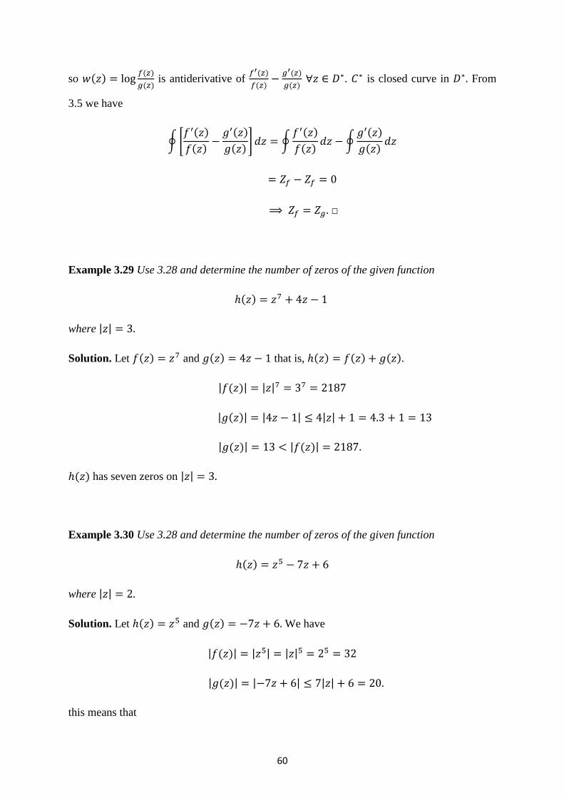
so ( ) ( )
( ) is antiderivative of
( )
( )
( )
( ) . is closed curve in From
3.5 we have
∮[ ( )
( )
( )
( )] ∮
( )
( ) ∮
( )
( )
□
Example 3.29 Use 3.28 and determine the number of zeros of the given function
( )
where | |
Solution. Let ( ) and ( ) that is, ( ) ( ) ( )
| ( )| | |
| ( )| | | | |
| ( )| | ( )|
( ) has seven zeros on | |
Example 3.30 Use 3.28 and determine the number of zeros of the given function
( )
where | | .
Solution. Let ( ) and ( ) We have
| ( )| | | | |
| ( )| | | | |
this means that

61
| ( )| | ( )|
Hence from 3.28 ( ) ( ) have five zeros inside | |
Theorem 3.31 (Open Mapping Theorem)
A nonconstant analytic function maps open sets onto open sets.
Proof. Let be open set. Now, we suppose that be analytic and nonconstant at
We have to show that ( ) is open. Let we choose such that we define new
function, that is ( ) ( ) is analytic in ( ) and it has no contain zero on
| | . Now, we will show that M be the minimum value of | ( )| on | | .
We will show that
( ) ( )
Let ( ). Then we have
| | | ( ) |
From 3.28;
( ( ) ) ( ) ( )
( ) and ( ) have the same number of zeros in ( ). Since ( ) has at least
one zero, then we can say that ( ) has at least one zero, as well. Since is arbitrary,
we must have
( ) ( ) □
Open Mapping Theorem has two results:
Corollary 3.32 (Maximum Modulus Principle)
Let be open and connected and is a holomorphic on U. Let such that
| ( )| | ( )| Then is constant.

62
Proof. Suppose that be open and connected and is a holomorphic on U. Pick
Since is bounded we have
| ( )| | ( )|
Since f is holomorphic function, by Cauchy’s Inequality, we have
| ( )|
| ( )| ( ) . Hence is constant. □
Corollary 3.33 (Maximum Modulus Theorem)
Let be bounded, open and connected. Let be a function which is continuous on
and holomorphic on U. Then the maximum value of | | must occur on .
Proof. Since is compact, | | must occur on . We have two cases.
Case 1: Suppose that f is constant. If is constant, result is obvious.
Case 2: Suppose that is nonconstant. Since is nonconstant from Maximum Modulus
Principle cannot have a maximum on U, so it must occur on □
3.3 Sequences of Holomorphic Functions
We will discuss a few result concerning sequence of holomorphic function. In this section we
will talk about Hurvitz’s Theorem. Because this is very useful for prove that the function is
injective. Additon to these we will talk about Montel’s Theorem. Because this is central key
for Riemann Mapping Theorem.
63
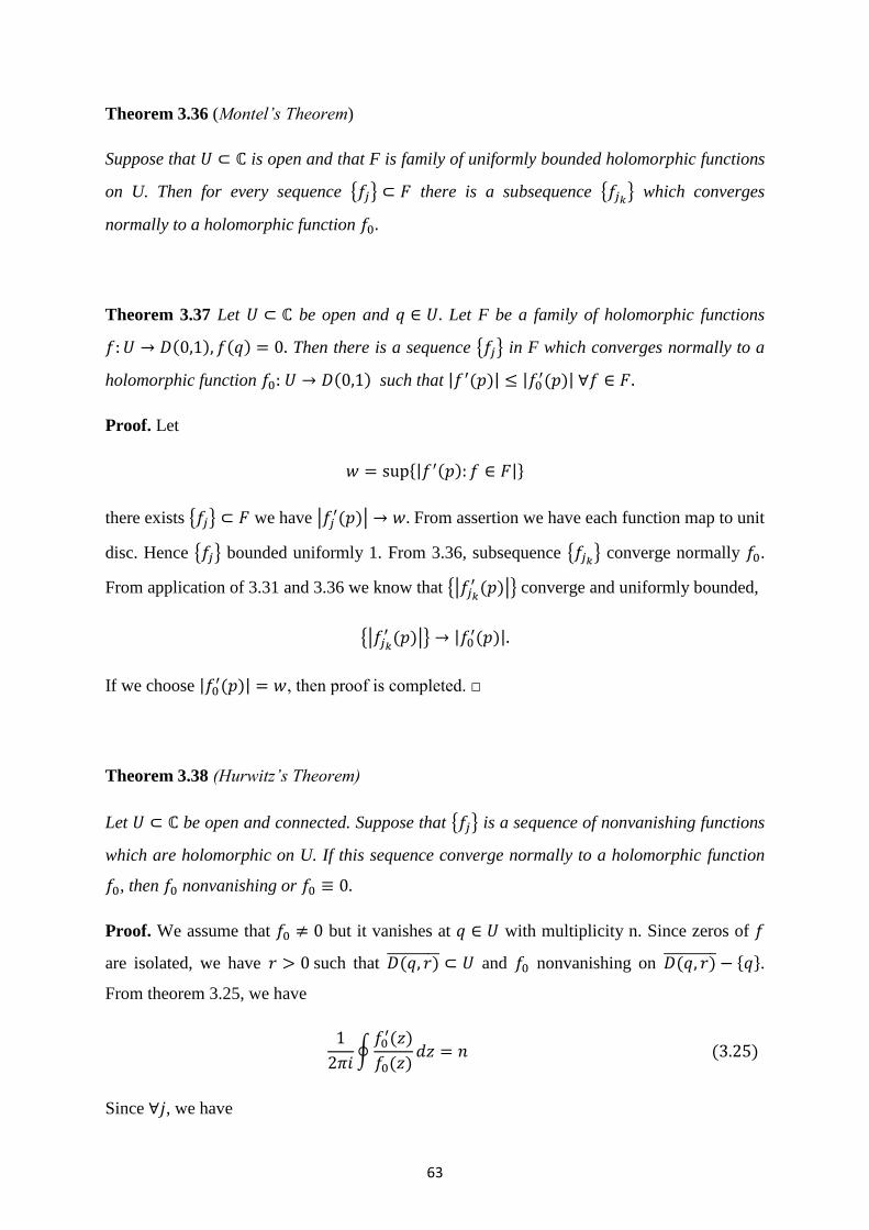
Theorem 3.36 (Montel’s Theorem)
Suppose that is open and that F is family of uniformly bounded holomorphic functions
on U. Then for every sequence { } there is a subsequence { } which converges
normally to a holomorphic function
Theorem 3.37 Let be open and Let F be a family of holomorphic functions
( ) ( ) Then there is a sequence { } in F which converges normally to a
holomorphic function ( ) such that | ( )| | ( )|
Proof. Let
*| ( ) |+
there exists { } we have | ( )| From assertion we have each function map to unit
disc. Hence { } bounded uniformly 1. From 3.36, subsequence { } converge normally .
From application of 3.31 and 3.36 we know that {| ( )|} converge and uniformly bounded,
{| ( )|} |
( )|
If we choose | ( )| , then proof is completed. □
Theorem 3.38 (Hurwitz’s Theorem)
Let be open and connected. Suppose that { } is a sequence of nonvanishing functions
which are holomorphic on U. If this sequence converge normally to a holomorphic function
, then nonvanishing or
Proof. We assume that but it vanishes at with multiplicity n. Since zeros of
are isolated, we have such that ( ) and nonvanishing on ( ) * +.
From theorem 3.25, we have
∮
( )
( ) ( )
Since , we have

64
∮
( )
( ) ( )
We know that { } and { } are converge uniformly to and on ( ) 3.25 must be
converge uniformly to 3.26. Its contradiction because n is nonzero positive integer. Hence we
have if then is nonvanishing. □
Now, we are going to talk about Schwarz Lemma and its corollary. They are very important
application for Riemann Mapping Theorem.
Lemma 3.39 (Schwarz Lemma)
Let ( ) ( ) be analytic function which maps the unit disc ( ) to itself. If
( ) then
| ( )| | | for | |
| ( )|
Proof. Let ( ) ( )
Then g is analytic for | | and it has singular point at
since ( ) It becomes analytic at 0 if we define
( )
( )
( )
fix , for | |
| ( )| | ( )
|
from Maximum Modulus Theorem for analytic g, it follows that | ( )|
for | | . Fix
( ) and let to get
| ( )|
This is true ( ) and
| ( )
| | |

65
| ( )| | | ( )
If | | then
| ( )|
| ( )| | ( )|
□
Corollary 3.40 ( ) ( ) conformal. There exists | | and ( ) such
that
( )
66
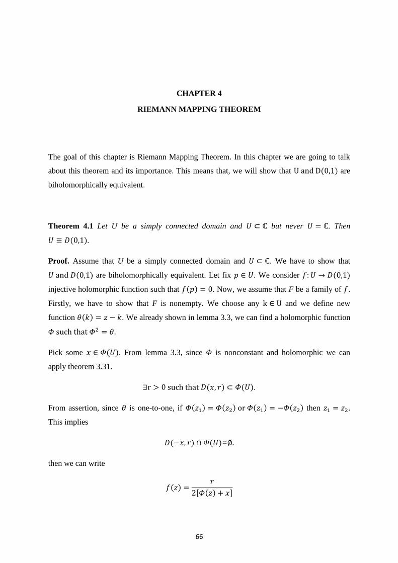
CHAPTER 4
RIEMANN MAPPING THEOREM
The goal of this chapter is Riemann Mapping Theorem. In this chapter we are going to talk
about this theorem and its importance. This means that, we will show that are
biholomorphically equivalent.
Theorem 4.1 Let U be a simply connected domain and but never . Then
.
Proof. Assume that U be a simply connected domain and . We have to show that
are biholomorphically equivalent. Let fix . We consider
injective holomorphic function such that . Now, we assume that F be a family of .
Firstly, we have to show that F is nonempty. We choose any and we define new
function . We already shown in lemma 3.3, we can find a holomorphic function
Pick some . From lemma 3.3, since is nonconstant and holomorphic we can
apply theorem 3.31.
.
From assertion, since is one-to-one, if then .
This implies
=
then we can write
[ ]

67
We have
| |
Hence .
We know that is one-to-one. Clearly, f is also one-to-one. Hence . Secondly,
since , in order to find any functions which are biholomorphic between .
We can use theorem 3.37 we have { } a sequence in F converge normally to
such that . So
| | |
|.
Now, we want to prove injectivity. Therefore we will apply theorem 3.38. If we show
is not identically zero then that is enough for injectivity. For every , we
define
{ }
From assertion we have for every , all are one-to-one. And also every nonvanishing on
{ }
This means that is one-to-one. In order to prove that we must show that is
onto. Suppose that is not onto then there exists which is not contained in image
of . Now we will see that Mobius transformations are very important to this. Now, we
consider new function on , that is
Clearly, is one-to-one and nonvanishing and maps to unit disc. Since U is simply
connected domain from lemma 3.3 we can find a holomorphic function
Now, we use Mobius transformations and we can define
68
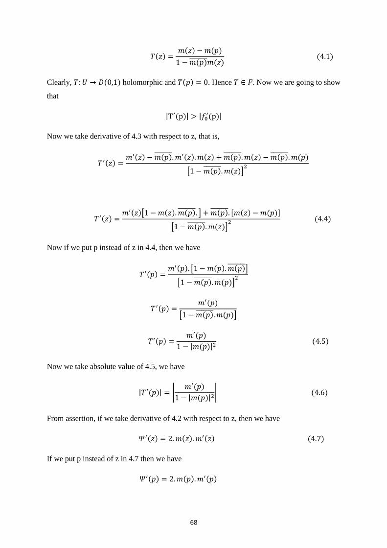
Clearly, holomorphic and . Hence Now we are going to show
that
| | | |
Now we take derivative of 4.3 with respect to z, that is,
[ ]
[ ] [ ]
[ ]
Now if we put p instead of z in 4.4, then we have
[ ]
[ ]
[ ]
| |
Now we take absolute value of 4.5, we have
| | |
| | |
From assertion, if we take derivative of 4.2 with respect to z, then we have
If we put p instead of z in 4.7 then we have

69
Clearly we have
Again from assertion we have . If we put p instead of z in 4.1, we have
Clearly we have
Now we put p instead of z in 4.2 then
If we put 4.9 in 4.10, then we have
We take absolute value both side of 4.11, we have
| | | |
If we take square root of 4.12 then we have
| | √| |
Now, we take absolute value of 4.2 then we have
| | | |
Note that from assertion
Now, we put 4.2, 4.5, 4.11, 4.13, 4.14 and 4.15 in 4.6 we have
| | |
| | | |
| ||

70
| |
| |
| | |
[ ]
[ ]
[ ] | | |
Since
| | |
| | |
| | |
| |
| | |
| | |
| | | |
| | |
| | |
| |
√| ||
We can see there
| |
√| |
So we have
| | | |
Its contradiction. is onto. Since one-to-one and onto then exists and holomorphic too.
So we have is biholomorphic functions which is . Proof is completed. □
Example 4.2 Let be biholomorphic. For { } such that
. We want a biholomorphic function which maps a to a zero.
Solution. We know that from 3.40 conformal. Then there exists | |
and such that

71
for this question we assume . And we have Mobius transformation;
We know that every Mobius transformations are biholomorphic and composite of mobius
transformations again biholomorphic. Clearly, . We can see there this is
one-to-one. Now, we have to show that this function takes a to zero.
Since , we have
□
Example 4.3 Find a conformal bijection mapping { | | } to
such that
to 0.
Solution. Let is analytic such that
(
)
we can see there the image of that
in second quadrant of . Let
Let . Since | | ,
| | | |
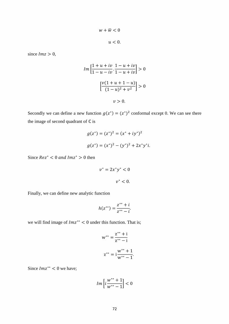
72
.
since
[
]
[
]
.
Secondly we can define a new function conformal except 0. We can see there
the image of second quadrant of is
.
Since then
Finally, we can define new analytic function
we will find image of under this function. That is;
Since we have;
[
]

73
[
]
This is . Now, we take compositon f, g and h;
* +
* +
We can see that
(
)
But we want to make 0. From 3.40 we have for any a in lower half plane then the map
Will suffice as a replacement for h. We can see there
(
)
If we change

74
Finally if we compose f, g and then we have
*
+
* +
This is conformal bijection and ( ) (
)
□

75
CHAPTER 5
CONCLUSION
Finally, instead of working in complicated spaces, Mobius transformations and Riemann
Mapping Theorem provides easier ways to find holomorphic functions between known
spaces. In my future life I would like work on this subject.

76
REFERENCES
[ ] Churchill, V. R., and Brown, W. J. (1990). Complex variable and applications. Second
edition. Singapore: Mc-GRAW-HILL, Inc.
[ ] Churchill, V. R., and Brown, W. J. (1996). Complex variable and applications. Sixth
edition. New York: Mc-GRAW-HILL, Inc.
[ ] Zill, G. and Shanahan, D. P. (1940). A first course in complex analysis with applications.
Canada: Jones and Bartlett Publishers.
[ ] Mathew, J. H., and Howell, R. V., (2006). Complex analysis for mathematics and
engineering. Fifth edition. United States of America: Malloy, Inc.
[ ] Ponnusamy, S. (2005). Foundation of complex analysis. Second edition. India: Alpha
Science Intl Ltd.
[ ] Stein, M. E. and Shakarchi, R. (2003). Complex analysis. United States of America:
Princeton U, Press.
[ ] Marsden, E. J., and Hoffman, J. M., (1987). Basic complex analysis. Second edition.
United States of America: W. H. Freeman and Company.
[ ] Gamelin, T. W., (2001). Complex Analysis with 184 illustration. New York: Springer-
Verlag New York Inc.
[ ] Churchill, V. R., and Brown, W. J., (1990). Complex variables and applications. Eight
edition. Singapore: McGraw-Hill Education.