Complete mm-Converter Measurement System including Noise ... · Joel Dunsmore , Agilent Fellow & Clive Barnett, Application Engineer Agilent Technologies October 2012 Complete mm-Converter

Joel Dunsmore , Agilent Fellow

&

Clive Barnett, Application Engineer

Agilent Technologies

October 2012

Complete mm-Converter

Measurement System

including Noise Figure

Workshop Outline

Most traditional mm-wave test systems test passive

devices and only measure linear s-parameters.

Today we are going to present a mm-wave system that can

offer a range of measurements suited for active devices....

....and present a system that can measure all of these

parameters including noise figure.

Workshop Agenda

• Typical mm-wave System Configurations

• mm-wave Applications

• Calibration

• Noise Figure

• Complete E-Band Converter Test System

Network Analyzer is the measurement engine.

Optional Test Set Controller interfaces to modules

THz Frequency Extenders provide frequency conversion and signal coupling

Basic mm-wave System Architecture

Vector Network Analyzer

Millimeter Wave Test Set controller

Frequency

Extenders

Device under test

Frequency

Extenders

Frequency

Extenders

Frequency

Extenders

PNA / PNA-X Network Analyzer

Key Enabling Features:

• 26.5 /43.5/50/67GHz versions

• Configurable Test set options

• Rear panel RF / LO Output

• Rear panel direct IF Access

• Test set controller interface

• Frequency Offset Capability

• Dual, spectrally pure sources with low phase noise

• Integrated pulse measurements

• Source Power Calibration & Receiver power leveling

• Broadband match corrected power Calibration

N5247A 4-Port PNA-X

Millimeter Wave Test Set Controller

• Provides LO & RF distribution to modules

• Provides DC power to modules

• 2-port (N5261A) and 4-port (N5262A) versions

• Flexible setup: measure multiple bands

• Mixer Measurements without external Sources

• Easily switch between PNA/PNA-X and mm-wave mode

PNA / PNA-X

Splitter RF Sw IF Switch Pwr

Ctl

LO Src1

Isolators

IO

RF Sw

Src2 IF x 5

Millimeter Wave Frequency Extenders

RF x 4 LO x 4 IF x 8 Pwr x 4

Four Port N5262 A Test Set Controller

Millimeter Frequency Extenders

• Broadband modules: 10M-110GHz

• Banded modules: 50 GHz ... 1 THz WR 15 50 – 75 GHz

WR 12 60 – 90 GHz

WR 12E 54 – 92 GHz

WR 10 75 – 110 GHz

WR 6 110 – 170 GHz

WR 5 140 – 220 GHz

WR 3 220 – 325 GHz

WR 2.2 325 – 500 GHz

WR 1.5 500 – 750 GHz

WR 1.0 750 – 1.1 THz

x N RF in

LO

in

Ref

IF

Test

IF

MM Test Port

RF RF LO

Banded Frequency Extenders

•Two Basic families Broadband or Banded Waveguide solutions

Millimeter Wave Configurations

4-port Broadband 4-port Banded

Broadband Single Sweep System

Single-sweep over 10MHz-110GHz

2-port & 4-port options

Uses 67GHz PNA & PNA-X

DUT Interface = 1mm coax

Features:

• Built-in Kelvin Bias Tees

• Broadband source leveling down to 70 dBm

• True differential Measurements

• Integrated Pulse measurements

• Mixer measurements

• Spectral Power Measurements

Banded Waveguide System Bands cover 50 GHz to 1THz

2-port & 4-port options with a Test Set Controller

2 Option without a Test Set Controller

Uses 26.5/40/50/67GHz PNA & PNA-X

DUT Interface = waveguide

Features:

• Source Power leveling up to 1.1 THz

• True differential Measurements

• Integrated Pulse measurements

• Mixer measurements

• Spectral Power Measurements

Configuration With Test Set Controller Configuration Without Test Set Controller

Waveguide Banded Solutions Configurations

OML PNA / PNA-X Banded Waveguide

Solution With Test Set Controller

VDI Banded Waveguide Solution

Without

Test Controller

Farran Banded Waveguide Solution With

Proprietary Test Controller

Workshop Agenda



– Compression

– Mixers

– Pulse

– IM Spectrum

– Materials

• Calibration

• Noise Figure


• Passives

• Amplifiers

• Mixers

• Semiconductors

• Antennas

• Materials

mm-wave Measurements

• S-Parameters (N-port,

Differential, Translated)

• Absolute power

• Gain compression

• Pulsed measurements

• Material parameters

• Time domain

mm-wave Devices mm-wave Measurements

• These measurements are typically associated with microwave

coaxial devices.

• But, by using a Test Set Controller and calibrating both for s-

parameters and power we can now start to offer more complex

mm-wave solutions.

mm-wave Measurements

mm-wave Compression Setup

mm-wave Compression Measurements

• Calibrate

• S-Parameters

• Source Power

• Receiver power

• Stimulus

•Sweep source power

• Measure

• S-Parameters

• Absolute power

• Compression

S-Parameters vs. Freq

Power & Compression vs. Power in

45dB power sweep at 98 GHz

mm-wave Mixer Measurements: Fundamental LO

RF Input

77 – 81 GHz

LO Input

78 - 82 GHz

IF Output 1 GHz

Fundamental

Mixer

mm-wave Mixer Measurements: Harmonic LO

RF Input

75-110 GHz

LO Input

9.35 GHz - 13.75 GHz

IF Output

100 MHz

Harmonic Mixer

IF = 1/6 * RF

LO= 1/8 * RF

mm-wave Mixer Measurements

Test Device: WR10 Module

75-110GHz RF

IF

9.4-13.8GHz

LO

• Calibrate

• S-Parameters

• Source Power

• Receiver power

• Stimulus

• Sweep the LO power

• Measure

• Match

• Power

• Conversion Loss

Conversion Loss vs. Freq

Input Power vs. Freq Input Match vs. Freq

Conversion Loss vs. LO power

mm-wave Pulse Measurements

Pulse: Techniques

Pulse: Measurement

• Calibrate

• S-Parameters

• Source Power

• Receiver power

• Stimulus

• Pulse generation

• RF Pulse modulation

• Swept frequency or power

• Measure

• S-Parameters

• Absolute power

• Pulse waveform

100us pulse power waveform at 98GHz

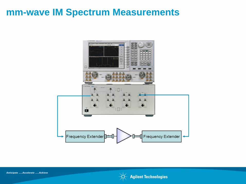
mm-wave IM Spectrum Measurements

mm-wave IM Spectrum Measurement

• Measurement Setup

• Assign Measurement class

• Set Path configuration to Thru path

• Setup the port power to correct

• Stimulus

• Set start and stop frequency

• Measure

• Input and output Spectrum

Input Spectrum

Output Spectrum

mm-wave Material

Measurements

Free space W-band system

Quasi-optical W-band system

mm-wave Material Measurements

• Calibrate

• 2-port S-parameters

(Methods such as

Gated-Reflect-Line)

• Stimulus

• Sweep frequency

• Measure

• Permittivity

• Permeability

• Sheet resistance

• Reflectivity

Workshop Agenda



• Calibration

– S-Parameter Calibration

– Power calibration

• Noise Figure


Calibration Interfaces

• Probe calibration

• Specific probe calibration software

• Uses basic and advanced cal methods (e.g. LRRM)

• Uses on-wafer cal standards

• Materials measurement calibration

• Specific materials measurement calibration software

• Uses basic and advanced cal methods (e.g. Gated-

Reflect-Time)

• Uses special free-space cal standards

•Waveguide calibration

• Uses basic calibration methods (SOLT, TRL)

• Uses rectangular waveguide calibration standards

Calibration Types

• 1-port Cal

• Short / Offset-Short / Match(1)

• 2-port "TRL-style" Cal

• TRL = Thru / Reflect / Line

• LRL = Line / Reflect / Line

• TRM = Thru / Reflect / Match(1)

• LRM = Line / Reflect / Match(1)

•2-port "SOLT-style" Cal

• Short / Offset Short / Match(1) / Thru

(1) Where "Match" is either a Load, Offset Load, or Sliding Load.

Quick-SOLT Calibration

• 2-port "QSOLT" • Measure Short / Offset-Short / Match(1) on one port • Measure zero-length thru between ports • Measuring four standards results in 2-port calibration • Useful for "mate-able" ports (e.g. waveguide)

• 4-port "QSOLT"

• Measure Short / Offset-Short / Match(1) on one port • Measure zero-length thru between three port pairs • Measuring six standards results in 4-port calibration

(1) Where "Match" is either a Load, Offset Load, or Sliding Load.

Power Calibration

Power Calibration Components to calibrate

• Source Cal

•Measures source output power

• Results in accurate output power at the

calibrated level

• Receiver Cal

•Measures receiver at calibrated power level

• Results in accurate, fast power measurements

• Receiver Leveling Loop

•Uses calibrated receiver to measure source

power

• Servo's the source to provide accurate output

power

Pout

Pin

Pout

level

Software

Power Sensor Cal

• A waveguide sensor is used to calibrate a

waveguide system

• Calibration process

• Waveguide sensor is connected to module

• Source power is calibrated

• Receiver power is calibrated using source

• Receiver is used to calibrate source power vs.

level

• Correction process

• Standard 12-term S-parameter correction

• Receiver is used to monitor source power;

Power level is adjusted using receiver leveling

Power Table Cal

• The power table defines the mm-module output

power vs. frequency when operated at its maximum

(clipped) output power.


• Enter the power table into the PNA-X

• Source power is set to maximum output

• Receiver power is calibrated using source

• Receiver is used to calibrate source power vs.

level





Max Power Table

Probe Calibration

• There are no wafer-based standards for power calibration


• Calibrate power at waveguide interface (using sensor or table)

• Calibrate S-parameters at waveguide interface

• Calibrate S-parameters at probe tips

• De-embed source and receiver power cal out to probe tips





Measurement Accuracy

Measurements accuracy is determined by

• Random errors

• Noise

• Connector repeatability

• Cable stability

• Drift & Stability errors

• Receiver

• Test set

• Systematic errors

• Compression & linearity

• Residual crosstalk

• Residual calibration errors

Calibration Errors

Residual calibration errors are determined by:

• Accuracy of calibration standards

• Load - match

• Offsets & Shims - length, match, loss

• Waveguide irregularities

• Burrs

• Rounded corners & sidewalls

• Flange edge and surface finish

• Aperture size

• Torque

• Cleanliness

• Alignment

Waveguide alignment (a.k.a. connector repeatability)

• Caused by vertical, horizontal, diagonal and rotational offsets(1)

• More sensitive at higher frequencies

• Use precision UG-387 flange (removable alignment pins)

(1) C. Oleson, A. Denning, "Millimeter Wave Vector Analysis Calibration and Measurement Problems

Caused by Common Waveguide Irregularities", Nov. 2000 ARFTG Conference Digest

Alignment Errors

D 1

D 2 D 5

D 4

D 3 D 6

Traceability

• S-Parameter cal

• Traceable to mechanical standards

• Some MM residual errors are large

• Power cal

• Uses calorimeter and S-parameter cal

• No industry-wide agreement on traceability

Workshop Agenda



• Calibration

• Noise Figure


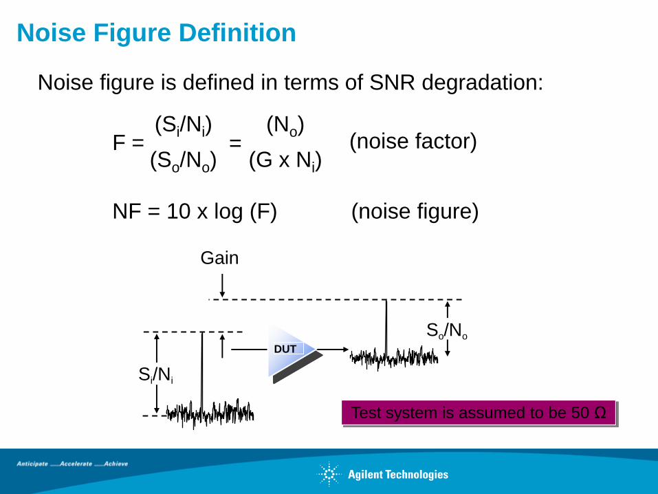
Noise Figure Definition

Noise figure is defined in terms of SNR degradation:

F = (So/No)

(Si/Ni) =

(No)

(G x Ni) (noise factor)

NF = 10 x log (F) (noise figure)

DUT

So/No

Si/Ni

Gain

Test system is assumed to be 50 Ω

Noise Figure Measurement Techniques

Y-factor (hot/cold source)

• Used by NFA and spectrum-analyzer-based solutions

• Uses noise source with a specified “excess noise ratio” (ENR)

• Measures noise figure and gain

Cold source (direct noise)

• Used by vector network analyzers (e.g. PNA-X)

• Uses cold (room temperature) termination only plus separate gain measurement

• Allows single connection S-parameters and noise figure (and more)

Excess noise ratio (ENR) = K

TT coldhot

290

Noise source

346C 10 MHz – 26.5 GHz

+28V

Diode off Tcold

Diode on Thot

Traditional Y-Factor Technique

Thot (on)

Tcold (off)

Pout (hot)= kBGa(Thot + Te)

Pout (cold)= kBGa(Tcold + Te)

Pout (hot)

Pout (cold) Y =

Thot – Y x Tcold

Y – 1 Te =

Noise Receiver

Te

290 Fsys = 1+

Calibration:

Noise Receiver

DUT

FDUT = Fsys – Frcv - 1

Ga DUT

Y-factor yields gain and noise figure

Unknown variables

Cold Source Technique

Pout= kBGa(Tcold + Te)

Pout

kToBGa

Fsys =

Noise Receiver DUT

Calibration:

Noise Receiver

FDUT = Fsys – Frcv - 1

GDUT

Need to know available gain very accurately

(Ga is function of S11, S22 and s)

Unknown variable

4-Port 43.5/50 GHz PNA-X Options 419, 423, H29

Noise source used

for calibration only RF jumpers

Receivers

Mechanical switch

C

R3

Test port 1

R1

Test port 4

R4

A D

rear panel

Pulse generators

1

2

3

4

Source 1

OUT 1 OUT 2

Pulse

modulator

Source 2

OUT 1 OUT 2

Pulse

modulator

Test port 2

R2

B

Noise receivers

10 MHz -

3 GHz

3 –

26.5

GHz

To receivers

LO

+28V

Test port 3

Signal

combiner +

-

Impedance tuner for noise

figure measurements

J9 J10 J11 J8 J7 J2 J1 J4 J3

35 dB 35 dB 35 dB

35 dB

60 dB

60 dB 60 dB 60 dB

PNA-X Versus NFA Comparison (Overlaid)

Vector calibration

Scalar calibration with

6 dB source attenuator


3 dB source attenuator


no source attenuator

NFA noise figure

NFA gain

PNA-X gain

Note: PNA-X NF traces

offset by one

graticule for clarity

• Is it possible to bring all these Applications together into one

complete system?

• Can we measure Noise Figure at mm-wave frequencies?

Complete mm-wave Measurement System

Workshop Agenda



• Calibration

• Noise Figure


E-Band Wireless Market is becoming

Commercialized

Wireless E-Band systems are now becoming prevalent.

They offer

• High data rate, 1Gb/s to University Campuses

• Driven by the increasing need for file, music and video sharing at Universities

The market is growing such that E-Band systems are now not just R&D

projects, but are generating requirements for 100’s of system components.

This means that customers expect commercial test systems to reduce test

time and unit cost

E-Band Requirements

Typical E-Band wireless systems include receivers.

Receivers are generally characterised by their Noise

Figure.

Which commercial test system can measure the

Noise Figure of an E-Band down-converter?

None!

E-Band Requirements

This measurement was traditionally attempted on a

Spectrum Analyser, UNCALIBRATED

.....well, until now...

How do you calibrate a test system to measure a

device that has mm-wave waveguide In and coax

RF Out?

E-Band Requirements

and bi-directionally?

and with a Single Connection?

How do you also measure mm-wave Gain,

Compression, Spurs, Return Loss at high

power ?

Splitter

Ext LO In

Tx Detector Out

Analog In

Introducing the new PNA-X Solution!

PNA_X can measure:

1. mm-wave Noise

Figure

2. Gain &

Compression

3. IMD’s

4. Spurs

5. Return Loss

6. Detector

Customer Need

A UK customer wanted to test an

E-Band Transceiver

• DUT is an E-band mm-wave to IF Rx

down-converter, and

• An IF to E-band mm-wave Tx up-

converter

• WR-12 Waveguide/SMA

• 6-port dut

• For Production.

x8

LO

x8

LO

Tx

Rx

12 GHz

9 GHz

84 GHz

74 GHz

9 GHz

4 GHz

Customer Requirement

Rx Path

• Noise Figure required

• 74 GHz in, 4 GHz IF

• Gain of Rx 20dB, NF 7dB

Tx Path

• High power output on Tx +26dBm

• Gain, Compression, LO Feedthrough,

Return Losses

• 12 GHz IF in, 84 GHz out

• Tx Detector voltage measurement

•Tx/Rx module with separate paths, but single

connection required

• Manufacturing, so test time under 4 mins per unit

• Customer supplied fixture and software control

Customer Device Birds Eye View

Push Fit

SMA

Connectors

DC

Rx LO Tx LO

Tx IF Rx IF

Customer Device and Fixture Side View

Tx LO Rx LO

Rx RF Tx RF

Fixture

IF/LO

All E-Plane

Bends. DUT

WR-12

Waveguide

Outstanding Problems

1. There is no commercial solution for Noise Figure

measurement on a mm-wave device

2. Tx high power output, requires attenuator to protect mm-

wave head, BUT we also need to measure Return Loss?

3. How do we measure in both Rx and Tx directions, with a

single connection?

Agilent Solution

Noise Figure at mm-wave

• Use a system with a 4-port

PNA-X & Test Set Controller

• Actually need to measure

Noise Power at 4 GHz IF

•Set up separate channels to

measure DUT Converter Gain

and Noise Power

• Fully error corrected Scalar

Conversion Gain and Scalar

NF

• Use on-board Equation

Editor to calculate NF on a 3rd

Trace

Agilent Solution

Can we measure Return Loss through Attenuators?

• A Low Power path was created, to measure the Return Loss and a High Power path with attenuation to measure saturated power and compression

• Mechanical switching to switch in/out High Power path

• Novel de-embedding used to de-embed the attenuator

OML, Tx 25dB

PAD

WG Straight

Fixture

OML, Rx

WG

Switch,

manual

Low Power

Path

High

Power

Path

DUT

Agilent Solution

How do we measure as a single connection?

• Use a mm-wave Test Set Controller

• With a 4-Port PNA-X

• Rear panel connections

• This enabled Port 2 on controller to drive the Tx mm-wave head, as well as using port 2 on PNA-X to measure the Rx IF R/L,

and NF.

PNA-X/Controller

E BandTransceiver

F

Ext

F

Ext

Signal

Generator

Signal

Generator

PSU + Control

Tx

O/P

Rx

I/P

Tx

IF

Rx

IF Tx

LO

Rx

LO

PNA-X Solution

Splitter

Ext LO In

Tx Detector Out

Analog In

Rx Measurements

Single Connection

• Return Losses

• IF Spurs

• Gain Compression

• Noise Figure

Tx Measurements

Single Connection

• Return Losses

• Gain Compression &

I/P, O/P Power

• IF Spurs

Test System

Test System

Conclusions

E-Band mm-wave transceivers are becoming commercialized

and as a result components are being tested in Production

The typical measurements are very demanding, and are not

typically done on VNA’s

The PNA-X system will measure all parameters including mm-

wave NF, with Error Correction.

The customer can now make all these measurements on a

device in under 4 minutes, compared to 15-20 minutes

manually

Documents

Complete mm-Converter Measurement System including Noise ... · Joel Dunsmore , Agilent Fellow & Clive Barnett, Application Engineer Agilent Technologies October 2012 Complete mm-Converter