Compilation and evaluation of a manualfor experimental nuclear engineering

Item Type text; Thesis-Reproduction (electronic)

Authors Goldstein, Jack, 1932-

Publisher The University of Arizona.

Rights Copyright © is held by the author. Digital access to this materialis made possible by the University Libraries, University of Arizona.Further transmission, reproduction or presentation (such aspublic display or performance) of protected items is prohibitedexcept with permission of the author.

Download date 26/06/2018 00:54:16

Link to Item http://hdl.handle.net/10150/551828

COMPILATION AND EVALUATION OF A MANUAL FOREXPERIMENTAL NUCLEAR ENGINEERING

byJack Goldstein

A Thesis Submitted to the Faculty of theDEPARTMENT OF NUCLEAR ENGINEERING

In Partial Fulfillment of the Requirements For the Degree ofMASTER OF SCIENCE

In the Graduate CollegeTHE UNIVERSITY OF ARIZONA

1 9 6 6

STATEMENT BY AUTHOR

This thesis has been submitted in partial fulfill­ment of requirements for an advanced degree at The University of Arizona and is deposited in the University Library to be made available to borrowers under rules of the Libraryo

Brief quotations from Volume I of this thesis are allowable without special permission, provided that accurate acknowledgment of source is madeo Requests for permission for extended quotation from or reproduction of this manuscript in whole or in part may be granted by the head of the major department or the Dean of the Graduate College when in his judgment the proposed use of the material is in the interests of scholarship. In all other instances, however, permission must be obtained from the authoro

Brief quotations from Volume XI of this thesis are allowable without special permission, provided that accurate ncknowledgmont of source is made• Requests for permission for extended quotation from or reproduction of this manuscript in whole or in part may be granted by the copyright holder.

SIGNED:

APPROVAL BY THESIS DIRECTOR This thesis has been approved on the date shown below:

Professor of Nuclear Engineering

ACKNOWLEDGMENTS

The author would like to express his gratitude and sincere appreciation to Dro Roy G. Post, without whose guidance and assistance this work would not have been possible. The help of many members of the Department of Nuclear Engineering, particularly Dr. Lynn Eo Weaver, Dr. Monte V. Davis, Dro Robert L. Seale, and Dr© Morton E. Wacks, is gratefully acknowledged* Appreciation is extended to the United States Army for the opportunity to complete this work. Finally, the author would like to recognize the invaluable contributions rendered by his wife and family. Their patience and understanding materially aided in the completion of this work0

iii

TABLE OF CONTENTS

LIST OF FIGURES ............... . . . . . . . . . . xLIST OF TABLES o . o o . . . . . * o . « o o . o o xiiABSTRACT o . o . o . . o o . * o * o o . o o . . « xxxx

VOLUME ICHAPTER

1. INTRODUCTION . . . . . . . . . . . . . . . . 12. EVALUATION OF BASIC RADIATION DETECTION

EXPERIMENTS . . . . . . . . . . . . . . . . . 4Experiment 1--Geiger-Muller and Proportional

Counters . . . . . . . . . . .Experiment 2— Portable Surveying Instruments Experiment ^--BF^ Neutron Detector ........Experiment 4— Semiconductor Detectors . . . . 10Experiment 6— Scintillation Spectrometry • • 12Experiment l4— Autoradiography . . . . . . . 14

3. EVALUATION OF ACTIVATION ANALYSIS ANDCOUNTING STATISTICS EXPERIMENTS . . . . . . . 1?Experiment ^--Counting Statistics . . . . . . 17Experiment 7--Flux Mapping by Foil Activation 19Experiment 8--Analysis of Mixtures of

Radioisotopes . . . . . . . . . . . . . . 21Experiment 9--Activation of Copper and Half-

Life Determinations..................... 224. EVALUATION OF EXPERIMENTS APPLYING

RADIOISOTOPE TECHNIQUES . . . . . . . . . 24Experiment 10--Removal Cross Sections . . . . 24Experiment 11--Chemical Separation ............ 26Experiment 12--Absorption of Beta Particles * 28Experiment 13--Decontamination of Surfaces . 30

Page

iv

vD *s

l ►£•

V

5. SUMMARY AND RECOMMENDATIONS . . ............. 32

Summary ' # © © © * © « * © * * * © * o o « * * 3 2Recommend ations # © © © © * © # © © © © © © * 3 3

APPENDIX A: ERRATA SHEET TO VOLUME II . © © . © . 35APPENDIX B: REVISED PROCEDURE FOR EXPERIMENT 11 . 38REFERENCES ........... © .......... » © . . . » . . 40

VOLUME IIINTRODUCTION................. © .......... © 1

PART ICHAPTER

1. NUCLEAR RADIATION AND ITS INTERACTIONS . . . 5Introduction . .Charged Particles Gamma Rays © © .Neutrons . © © ........ © . . . . © . . . . 10Radioactive Decay 10

2. RADIATION SAFETY ............................ 12Introduction............................. 12Biological Effects © © ........ © .......... 12Radiation Units as Applied to Dosimetry . . . 15Allowable Dose and Dose Rates » . . . . © © o 19Radiation Protection . . . « . . . . . . © 21Radiation Monitoring Instruments . . . © . © 22Rules for Laboratory Operation . . « . © . . 23Decontamination . . . o . . . . . . . . © . © 26

3© ANALYSIS OF ERRORS » . . . . . . . . . . . © 2?Introduction . . . . . © © * © © # . . # . © 27Definitions . # © . . . . . © . © . © . © © © 27Classification of Errors . . . . © . . . © . 28Errors from Radiation Detection Equipment . © 29Errors from Radiation Measurements . . . © . 30

TABLE OF CONTENTS--ContinuedPage

~v

lUl vi

viTABLE OF CONTENTS— Continued

4. COUNTING STATISTICS . . . . . . . . . . . . o 31Page

Introduction . . . . . . . . . 31The Binominal Distribution ............... 32The Poisson Distribution . . . . . . . . . . 34The Normal Distribution . 36Standard Deviations............ 37Propagation of Errors . . . . . . . . . . . . 40

5. REPORT PRESENTATION . . . . . . . . . . . . . 43PART II

EXPERIMENT 1: GEIGER-MULLER AND PROPORTIONALCOUNTERS . . . . . . . . . . . .......... . 51Purpose .......................Theory . . . . . . . . . . . .Apparatus .....................Procedure * ........ ..Results and Presentation of Data Questions and Problems . . . . Selected References . . . . . .

515154555859 59

EXPERIMENT 2: PORTABLE SURVEYING INSTRUMENTS . . . 60Purp o s e . . . . . . . . . . . .Theory . . . . . . . . . . . .Apparatus . ............. ..Procedure . . .................Results and Presentation of Data Questions and Problems . . . . Selected References ........ .

606063636566 66

EXPERIMENT 3*. BF^ NEUTRON DETECTOR 68Purpose .. ................. . . . . . .Theory . . . . . . . . . . . . . . . . .Apparatus . . . . . ........ . ........Procedure . . . . . . . . . . . . . . . .Results and Presentation of Data . . . .Questions and Problems . . . . . . . . .Selected References . . . . . . . . . . .

68687070727273

EXPERIMENT 4: SEMICONDUCTOR DETECTORS 74Purpose 74

viiTABLE OF CONTENTS— Continued

Theory App nratus ProcedureResults and Presentation of Data Questions and Problems . 0 0 . Selected References . . . o .

EXPERIMENT 5: COUNTING STATISTICSPurpose ........ 0 0 . 0 . . .Theory • © • e # « • • o 0 • •ApparatusProcedure . . . © « . . . . .Results and Presentation of Data Questions and Problems = . . .Selected References = . © . . .

EXPERIMENT 6 : SCINTILLATION SPECTROMETRYP u r p o s e o < « « * o * » o » . © < Theory © © • • © © © © • • • • <Apparatus . © ........ .. « © © ,Procedure © © © • © • © • o o © < Results and Presentation of Data Questions and Problems . . © . , Selected Referencos . . © . © . ,

EXPERIMENT ?: FLUX MAPPING BY FOIL ACTIVATIONPurpos c * » © # © # » © # © # # « Theory • • • • © © © © © © © • « Apparatus © • © • © © • • © • © < Procedure © , . . © . . . © © © , Results and Presentation of Data Questions and Problems © © © . « Selected References . . . © © © ,

EXPERIMENT 8: ANALYSIS OF MIXTURES OFRADIOISOTOPES . © .......... ..Purpose © • • # # 0 * © * * © © "T h e o r y .......... © . . . . © .Apparatus • © • © • • • © • • • <Procedure ........ © * . * * © ,Results and Presentation of Data Questions and Problems . . . © .Selected References . . . . . .

Page747677 79798081818181818284848585859192 92 9494959595100100101101102

103103103104 104 106 107 107

viiiTABLE OF CONTENTS— Continued

PageEXPERIMENT 9: ACTIVATION OF COPPER AND HALF-LIFE

DETERMINATIONS . . . . . • ° • • ° • • 108P m r p O S © e o o e e o o e o o • 0 © . 0 e O O 108Theory . . . . . . 108Apparatus o o # * . . . # IlkProcedure 0 * 0 . o 0 . o IlkResults and Presentation of Data o • • 0 ♦ 115Questions and Problems • © . o o . • • o o 115Selected References • © • © c . o 116

EXPERIMENT 10: REMOVAL CROSS SECTIONS 117Purpose O O e O O 117Theory # » # * # * * # © » 0 • © • © • 117Apparatus . . . . . . . . . © © • © • . 119Procedure . . . . . . . . 119Results and Presentation of Data • • o o o • 121Questions .md Problems . • • o • o . • 121Selected References . . . . • • ° ° • • 121

EXPERIMENT 11: CHEMICAL SEPARATION „ . 122Purpose ................. .. O O 0 O 122T h e o r y .......... © . © © • • © • © 122Apparatus ............... © * * # © • © • o 123Procedure o o « .......... O 0 • 12kResults and Presentation of Data • • o e • 125Questions and Problems © • 125Selected References © • • © • • o ° • 126

EXPERIMENT 12: ABSORPTION OF BETA PARTICLES ° • • 127PurpOSe o o o o o e o e e o * * © o e o . 127Theory • • • © © © • © • • • • • • o . o © 127Apparatus © © • © • • © • o © O • o • o • . 129Procedure © . . . o o . . 0 . 0 O 130Results and Presentation of Data O O e O 130Questions and Problems © © © © • o e O 0 # 131Selected References • © • , • 131

EXPERIMENT 13: DECONTAMINATION OF SURFACES • • • 132Purpose . . o o . . . c . . • o • 0 0 o 132Theory . . . . . . o o . . © o • • e • O . o 132Apparatus o o o o . o . o . o 13kProcedure o . o o . . . 0 . 0 . 0 • . o 0 • . 135

ixTABLE OF CONTENTS— Continued

PageResults and Presentation of Data # • # • # < > 135Questions and Problems IjGSelected References . o . e o . . # * o o o . 136

EXPERIMENT ik: AUTORADIOGRAPHY . . . 0 0 0 0 . . . 137Purpose . . . . . . o . *Theory o # * o * o * # # # Apparatus . . . . . 0 0 .Procedure . < , 0 . 0 . . 0 0Results and Presentation of Questions and Problems o o Selected References • © o •

. c ............ 137• • • © • • * • • 137o e e o o e o e e 1 3 ^

• • • o o e e e e 1 3 ^

Data • © © © • © 139e o e o e e o e e 1 3 9

• o o o o e e o o 1 3 9

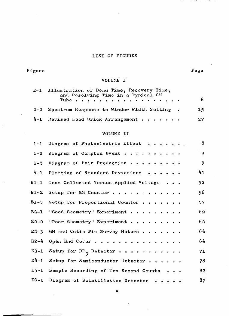
LIST OF FIGURES

VOLUME I2-1 Illustration of Dead Time, Recovery Time,

and Resolving Time in a Typical GM Tub e 6

2-2 Spectrum Response to Window Width Setting . 154-1 Revised Lead Brick Arrangement . . . . . . 27

VOLUME II1-1 Diagram of Photoelectric Effect .......... 81-2 Diagram of Compton Event . . . . . . . . . 91-3 Diagram of Pair Production . • ............. 94-1 Plotting of Standard Deviations . . . . . o 4l

El-1 Ions Collected Versus Applied Voltage . . . 52El-2 Setup for GM Counter . . . . ............. 5&El-3 Setup for Proportional Counter . . . . . . . 57E2-1 "Good Geometry" Experiment . . 0 0 0 . . 0 . 62E2-2 "Poor Geometry" Experiment .......... . . . 62E2-3 GM and Cutio Pie Survey Meters . . . . . . . 64E2-4 Open End Cover . . . . . . . . . . . o . 64E3-I Setup for BF^ Detector 0 0 0 0 . . • • . . . 71E4—1 Setup for Semiconductor Detector .......... 78E5-1 Sample Recording of Ten Second Counts . . . 82E6-1 Diagram of Scintillation Detector o . o . . 87

Figure Page

x

LIST OF FIGURES— Continued

E6-2 Cobalt 60 Gamma Spectrum . . . . . . . 90E6-3 Scintillation Detector with Recording

Spectrometer 93E8-1 Scintillation Detector with Multichannel

Analyzer 105E9-1 Semi-Log Plot for Half-Life Determinations • 110E9-2 Pcierls' Method for Half-Life Determinations 110E9-3 Two Point Method for Half-Life Determina­

tions o . . o ............. . . . o s . 113E10-1 Experimental Arrangement for Removal

Cross Sections . 120E12-1 Pure Beta Absorption Curves . . . . . o * 128E12-2 Feather Plot o o o o . o o . o o . . . . . . 129

xi

Page

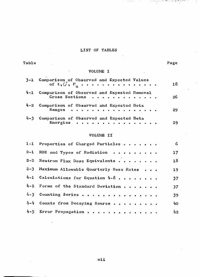
LIST OF TABLES

3- 1

4- 1

4-2

4-3

1-12—12-22-34-14-24-34-44-5

TableVOLUME I

Comparison of Observed and Expected Values of 1 1 O ) Pu « • 0 0 0 0 * 0

Comparison of Observed and Expected Removal Cross Sections • * o * o o o * o « » * o

Comparison of Observed and Expected Beta Ranges 0 * * 0 0 0 0

Comparison of Observed and Expected Beta Energies o o o * # * * o * * # o o o * *

VOLUME IIProperties of Charged Particles . . . . .RBE and Types of Radiation • * • • • • • • •Neutron Flux Dose Equivalents .Maximum Allowable Quarterly Dose Rates o o • Calculations for Equation 4-8 . . o o . e . o Forms of the Standard Deviation o . . . . . .Counting Series . . . . . . . . . . .Counts from Decaying Source . . . . . . .Error Propagation...............*

18

26

29

29

61718

19 37 373940 42

Page

xii

ABSTRACT

A laboratory manual for an introductory course in experimental nuclear engineering was written and evaluated for the Nuclear Engineering Departmentt University of Arizona. The manual was designed to acquaint students with the basic understanding necessary for experimental research in nuclear engineering.

Evaluation of this manual is based in part on its use in a course entitled "Experimental Nuclear Engineering I," offered by the Nuclear Engineering Department, University of Arizona during the fall semester 1965. Observations of a series of fourteen experiments and of the laboratory reports that were submitted upon the completion of each experiment were madeo Analysis of the experimental results achieved shows that this manual achieves the objectives for which it was designedo

xiii

VOLUME I

EVALUATION OF MANUAL

CHAPTER 1

INTRODUCTION

There have been many textbooks written in the field of experimental nuclear engineering. Such books as "A Manual of Experiments in Reactor Physics" by Frank A. Valente, "Radioisotope Techniques" by Ralph To Overman andII. Mo Clark, "Experimental Reactor Analysis and Radiation Measurements" by Donald D . Glower, and "Nuclear Reactor Experiments" by Barton J. Hoag all have added greatly to nuclear engineering as a field of engineering education. Effective textbooks are available in this field, however, the need for a well-organized introductory laboratory manual, coordinated with appropriate text material and containing a wide selection of experiments has not been met o

Future advancements in the field of nuclear engineering depend greatly upon experimental research. If future individual research is to be effectively conducted, it is essential that the student understand the basic principles of experimental measurements in nuclear engineering.

If an experiment is to be effective, it is imperative that the person conducting the research insure

1

2that the experiment will measure the quantity that has been specified, that the conduct of the experiment will not influence the results, that the experiment will be con­ducted with sufficient accuracy and sensitivity, and that the results of the experiment can be interpreted. This manual, Volume XI of the thesis, provides this understand­ing if the experiments presented are successfully completed and adequately analyzedo

Volume IX is written in two parts« Part I contains a brief review of the fundamental aspects of modern physics important in nuclear engineering experimentation, a review of the fundamentals of radiation safety, a discussion pertaining to analysis of experimental errors, and a format for report presentation. The experiments in Part II are designed to teach the student basic types and character­istics of radiation, methods of radiation detection, characteristics and operation of principal radiation detection equipment, identification of radioisotopes, radiation safety procedures, and the use of radioisotopes to perform specific laboratory experiments.

The evaluation, Volume I of this thesis, is intended to determine the effectiveness of the manual in meeting the outlined objectives*

An evaluation of any text or manual cannot be accomplished satisfactorily until it is used in teaching. Twelve students, two second year graduate, 8 first year

3graduate, and 2 senior undergraduate, enrolled in a course using this manual during the fall semester 1965* Results of the experiments conducted by these twelve students, combined with the twelve sets of fourteen laboratory experiments, provide insight into the effectiveness of the manual in meeting the objectives®

Each chapter in Volume I contains an evaluation of a particular group of experiments o Experiments 1, 2, 3, 4, 6, and l4 deal with basic radiation detection techniques and are evaluated in Chapter 2® Activation analysis, stripping techniques, and counting statistics are stressed in Experiments 5, 7, 8, and 9 and are evaluated in Chapter 3• Finally, Experiments 10, 11, 12, and 13, dealing with applications of previously mastered techniques of radio­isotope measurement and handling, are evaluated in Chapter4®

In all fields of engineering, particularly in nuclear engineering, where so much vital research and development remains to be done, it is extremely important that a student be competent in methods of experimentalresearch

CHAPTER 2

EVALUATION OF BASIC RADIATION DETECTION EXPERIMENTS

EXPERIMENT 1— Geiger-Muller and Proportional CountersExperiment 1 was designed to acquaint the student

with the characteristics, the operation, and the uses of two basic radiation detectors, the Gciger-Muller and proportional counters. Additionally, emphasis was placed on methods for determining the resolving time of the Geiger-Muller counter.

The most important aspect of any initial nuclear engineering laboratory experiment is to insure that there is a basic understanding of the types of radiation being measured and how these measurements are accomplished © This is achieved by use of specific questions as part of the laboratory report. Correct answers to these questions depend upon an understanding of the theory of the experi­ment . Specifically, these questions require analysis of the type of gas used in the experiment, a discussion of background radiation, quenching, and chamber flushing, and an analysis of the advantages of the particular detectors used in the experiment. Another important aspect of any initial laboratory experiment is to familiarize the students with the basic electrical equipment to be used

5throughout the course. The students connected all electrical equipment used in this experiment from two photographic-type block diagramso These diagrams proved to be valuable training aids and there were few problems encountered in initial equipment setup»

An error in terminology resulted in a great deal of confusion in this experiment <, The term "dead time" was used to describe the minimum time interval between events which can be registered in a counterc Actually a more common term used in the literature to describe this event is "resolving time." Confusion on this point can be corrected easily if the "dead time" referred to throughout Experiment 1 is changed in all places to "resolving timeo"

Additionally, a paragraph should be added to the theory section of Experiment 1 to define accurately dead time and recovery time as well as resolving time• Dead time (t^) is the time, following an event in the tube, in which the tube can give no pulse or has no response to an ionizing event o The time required for the complete recovery of the pulse size after the end of the dead time interval is known as the recovery time (t^).

If the counting system in use has a very sensitive voltage amplifier, the resolving time (R) for the system approaches t^. For a less sensitive tube, the resolving time (R) lies between t . and t , + t .

6Inclusion of Figure 2-1 to Experiment 1 will

further clarify these points c

Maximum Resolving Time Minimum

Resolving Time Recovery 1 Dead Time (t ,) (t )

0 100 200 300 4oo 500 GooTime (p. sec)

Figure 2*1. Illustration of Dead Time, Recovery Time, and Resolving Time in a Typical GM Tube

This figure is redrawn from page 126 of Nuclear Radiation Detection by Price (See Reference 12).

The plateaus for the GM and proportional counters agree closely with those given in Price (See Reference 12). An average resolving time of 425 microseconds was found in this experimento This value will normally be between 300 and 700 microseconds depending on the sensitivity of the voltage amplifiero

EXPERIMENT 2--Portable Surveying InstrumentsThis experiment illustrated the use of portable

radiation surveying instruments for area surveys. Addi­tionally, the attenuation of gamma photons and the effects of geometry on radiation detection were considered.

Use of the portable detectors was adequately illustrated by having each student prepare a laboratory diagram and conduct a survey of the laboratory using a portable GM counter o Sources of known intensity were placed throughout the laboratory to check on the accuracy of the survey conducted. This emphasized the necessity of careful monitoring in an area of suspected radiation. Correct procedures to follow in the use of portable survey instruments were stressed throughout the laboratory period and summarized in questions 1, 2, and 3 on page 66 in the laboratory manual© These questions basically determine whether or not the students are aware of the advantages and disadvantages of certain portable detectors and emphasize the correct procedure used in operating these detectors ©The fact that all students performed exceptionally well in the laboratory and answered questions 1, 2, and 3 correctly in their reports was evidence that these key points were clearly understood.

Early in this introductory course it is necessary to understand the concept of attenuation of photons from a well-collimated beam of monoenergetic photons and the

8factors that describe the geometry under which an experi­ment was conductedo A design that allows virtually no Compton scattered photons or annihilation photons, if pair production is involved, to reach the detector is one type of experimental arrangemento If, however, a cylindrical shell is placed around the source and the detector is left unshielded, then the experimental arrangement would allow Compton scattered photons or annihilation photons to reach the detectoro In this type of arrangement the intensity at the detector is greater than the uncollided intensity and the ratio of the observed to the uncollided intensity is sometimes called a build-up factor.

Build-up factors determined in this experiment were compared at p^x = 1 with those values listed in Goldstein (See Reference 7)•

With a sot of iron absorbers the average percentage error between the value of p^x determined experimentally and that given in Goldstein (See Reference 7) was 4.3 percent.

With a set of aluminum absorbers the percentage error could not be found at U x = 1 since, due to a mis- calculation in designing the aluminum absorbers, there was not an aluminum absorber available of sufficient thickness to give Pqx = 1o This would have required an absorber thickness of 2<>38 inches when in fact the maximum thick­ness available was 0*884 inches * Therefore, a comparison

9with Goldstein (See Reference 7) was taken at = 0.372and the average percentage error was found to be 6.25 percento

EXPERIMENT 3--BF. Neutron Detector

The purpose of Experiment 3 was to illustrate the basic principles involved in neutron detection. Addi­tionally, an operating plateau for the boron trifluoride (BF^) neutron detector was determined.

This experiment was relatively simple and was performed with a minimum amount of difficulty. The operating plateau of the modified BF^ was found within 5 percent of the plateau given in Price (See Reference 12).

There was, however, some confusion in the answers given to questions 1 and 2 on page 12 of the laboratory manual. Three of the twelve students interpreted question 1 as requiring only the energy of the fast neutrons. Six of the twelve students only gave the absorption cross section of cadmium for thermal neutrons. In fact, questions 1 and 2 required that the total neutron energy spectrum for Pu-De neutrons be plotted as well as the absorption cross section of cadmium for this spectrum. Future emphasis should be placed on these points.

This experiment should be expanded to include, not only a BF^ neutron detector but also, a fission counter. Fission counters are frequently used as neutron detectors

10in experiments involving nuclear reactors. The large energy released per reaction makes it possible to dis­criminate against much larger fluxes of gamma rays than with detectors employing the (n, oc) or similar reactions o This latter property makes the fission chambers particu­larly useful for the measurement of the small neutron fluxes which are present in the start-up and shutdown of a reactor. These neutron fluxes are accompanied by large gamma ray fluxes so that discrimination becomes very important. For this type of application BF^ detectors are unsuitable. Since a subsequent laboratory course will have several reactor experiments that will use fission counters t it is important to acquaint the student with the characteristics and method of operation of this type of neutron detector.

In this experiment, after the data has been taken with a DF^, the BF^ should be replaced with a fission counter and a plateau curve determined„

In addition to adding the above data to the theory section of Experiment 3» the requirement to determine the sensitivity of the fission counter should be added as question 9 on page 73 of the manual.

EXPERIMENT 4— Semiconductor DetectorsSemiconductor detectors have many advantages in

experimental nuclear engineering as radiation-particle

detectors. They arc small, rugged, fast, simple, and do not require high voltage supplies, cooling, windows, or flow of gasseso Because of their increasing importance, an introductory experimental nuclear engineering course should contain at least one experiment in the theory and use of semiconductor detectors.

The students were required to use a photographic- type block diagram to make all electrical connections and once again this proved to be a satisfactory teaching aid.

One major problem occurred in this experiment due to the energies of the alpha particles emitted from the available source. The alpha emitting source was Cm with alpha energies of 5.76 and $.80 Mev. The range of 5-6 Mev alpha particles in air at 25°C and 760 mm of Hg is approxi­mately six centimeters. In this experiment the distance from the source to the detector was much less than six centimeters and consequently there was very little attentuation of the alpha particles by any amount of air in the chamber. Therefore, the variation in counts recorded as a function of applied pressure stems mostly from statistical fluctuations.

This problem could have been corrected in one of three ways» Another alpha source with a reduced alpha energy could have been used. If another source were not available, the size of the vacuum chamber could be increased. Instead of either of these two corrections, a sheet of

11

paper could have been placed between the alpha source and the detector <,

There were a number of questions during the labora­tory period concerning the effect of the bias voltage adjustment. The results and presentation of data section should be expanded to include a graph of counts recorded versus bias voltage applied. After this curve has been plotted its physical significance should be discussed starting from the zero voltage level and continuing to the high bias voltage region.

EXPERIMENT 6— Scintillation SpectrometryThis experiment was designed to study scintillation

spectrometry by analyzing known and unknown gamma ray spectra.

Use of the C o ^ source as the calibration spectrumled to some difficulty in plotting a calibration curve ofenergy versus base line. The two photopeaks obtained forC o ^ at 1o17 and 1.33 Mev are so close together that abetter procedure would have been to use both Co^® and

137as calibration spectra = Ce J 1 has a photopeak at 0067 Mev. By using this value in conjunction with the C o ^ values of lol7 and 1.33 a wider range and more accurate calibration curve could have been obtained.

The discussion given on page 89 and 91 of the laboratory manual of pair production resulted in some

12

initial confusion. It should be emphasized that several things can happen to the annihilation photons from the positron that results from a pair-production event. Both photons can escape the crystal creating a pair production peak 1.02 Mev below the photopeak. One photon can escape the crystal and the other undergo a photoelectric capture, in which case the pair production peak would appear 0»511 Mev below the photopeak. If both photons are absorbed in the crystal this energy would be included in the photopeak„

The illustrative C o ^ spectrum shown on page 90 of the laboratory manual should be modified to show the "sum" peak of 2.50 Mev. This can easily be accomplished by use of a 1024 channel multichannel analyzer and an x-y recordero

There were some problems encountered in this experiment with the window width setting on the recording spectrometer and with the subsequent answer to question 1 on page 94 of the laboratory manual« This question requires a discussion of the manner in which the window width setting on the radiation analyzer of the recording spectrometer would affect experimental results. The theory section of the experiment should be expanded to include a short discussion on the necessity for correct window width setting. For examplet in the C o ^ spectrum there are photopeaks at 1.17 and 1.33 Mev• If the window width setting were too large these peaks would tend to converge

13

and ultimately become indistinguishable. On the other hand, if the window width setting were reduced, continually finer resolution would be obtained. This is desirable, up to a point. If the resolution is allowed to become too fine the character of the vertical plot would be lost. The optimum setting would, therefore, be one which allowed a clear resolution of the peaks in a given spectrum, but does not resolve the energies into such small bands that the number of counts per channel becomes insignificant.

This point can be illustrated by means of the graph shown in Figure 2-2. Suppose that one had a total number of 100 counts recorded for an energy band of from 0 to 1.0 Mev. If the window width were sot to discriminate only every 0.5 Mev, the results would be as shown by A in Figure 2-2. Here the peaks tend to converge and ultimately become indistinguishable. If the resolution is too fine, and instead of discriminating every 0.5 Mev, it is done every 0.005 Mev, the results would be as shown by D in Figure 2-2.

EXPERIMENT l4— AutoradiographyPrinciples of autoradiography, the determination

of the distribution of the radioactivity in a specimen by use of photographic emulsions were emphasized in this experiment.

Numb

er o

f Co

unts

15

Energy-

Figure 2-2o Spectrum Response to Window Width Setting

16No difficulties were encountered and the experiment

served to illustrate the many uses of this type of radia­tion detectoro

The second step of the procedure given on page 138 of the manual indicates that the aluminum-indium packets used in this experiment should be irradiated to an inten­sity of approximately 5 mr/hr. This level of radiation is higher than that required for the experiment and is above the allowable radiation limits for a laboratory similar to the one used for the conduct of the experiment. The radiation level of the packets should not be higher than 2.5 mr/hro

CHAPTER 3

.......

EVALUATION OF ACTIVATION ANALYSIS AND COUNTING STATISTICS EXPERIMENTS

EXPERIMENT 5— Counting StatisticsThis experiment was very closely coordinated with

the counting statistics information presented in Chapter 4 of the laboratory manual. In Chapter 4 the need for statistical analysis in processes associated with counting, the types of probability distributions, and the methods of using these distributions in laboratory procedure are briefly describedo

The close association between the "Results and Presentation of Data" section, of this experiment and the information in Chapter 4 presented some initial problems in the preparation of the laboratory reports• These problems can be reduced if there is a slight rearrangement of the numbering sequence in this section of the experi­ment o The third requirement, a plot of P^ (probability that a mean value m is missed by an amount u), experimental and theoretical, versus x, should not come until after step 14 in the sequence» It is not until step l4 that the experimental values for P^ are first calculated.

Questions 8, 12, and 15 of the "Results and Presentation of Data" section require a comparison between

17

18experimental and theoretical values for t (average time for a number of counts), 0 (standard deviation), and (probability that a mean value m is missed by an amount u)o

The results expected for t, O', and are 0.218, 105» and 0.62 respectively. These results are obtained from Chapter 4 of Part I in the laboratory manual. A chi squared analysis can be used to compare observed and expected results for P^ and t. An F test can be used to compare observed and expected results for O' • Table 3-1 lists observed and expected results with the value of chi squared for Py and t as well as the value of F for O'•

Table 3-1Comparison of Observed and Expected

Values for t,0» and P^

Item Expected Observed X F

t 0.218 0.236 0.0040.242

O' 105 99 <190p 0 oG2 0.69 0.014u 0 0 6 8

Therefore, based upon a chi squared analysis, thevalues observed for t and Pu can be expected to be withinthe statistical distribution 95 and 88 percent of the time

- ' '' :

19respectively. Since F is less than 1, the values obtained for (j are within the same population as the expected reading.

Experimental errors could be reduced if more samples were taken. However, this is not recommended since the length of this experiment is already excessive and the results obtained are sufficiently accurate to illustrate the desired points.

EXPERIMENT 7— Flux Mapping by Foil ActivationActivation of foils is a basic method by which many

nuclear engineering experiments are conducted. These experiments include, among others, flux mapping and cross section analysis. This method is based on the fact that certain stable isotopes, upon capturing a neutron, are transformed into radioactive isotopes. This experiment was designed to illustrate foil activation by measuring the flux in a neutron howitzer.

Some initial confusion existed with reference to the proper type of foil to select for a given experiment. The theory section of this experiment should be expanded to include the necessary considerations in selecting the correct foil for activation. These considerations include the estimated neutron energy level of interest, the magnitude of the neutron flux density to be measured, the total exposure required before foil activity can be

20measured, the accuracy required in the final result, and the availability of foil materials. This analysis will result in the selection of a foil which is available, which has the appropriate activation cross section and half-life, and which has these parameters known to the desired accuracye It should be realized that many activation cross sections are unknown, particularly for neutrons in an energy range other than thermal•

Question 3 on page 102 of the laboratory manual pertaining to the cadmium ratio resulted in some dif­ficulty. Four of twelve students stated that the cadmium ratio should be lower at the edge of the howitzer than at the sourceo Actually, the cadmium ratio, defined as the ratio of the activity of a foil exposed to the neutron flux to the activity of an identical foil surrounded with cadmium and exposed to the same flux, is higher at the edge than at the source• This cadmium ratio actually approaches infinity as all the neutrons approach thermalization. Cadmium cut-off occurs at 0.4 ev. In other words, the cadmium essentially stops all neutrons below its cut-off energy and is nearly transparent to neutrons of greater energy. A cadmium ratio of 10 and 100, therefore, represents a thermal flux equal to 90 and 99 percent of the total flux, respectively.

EXPERIMENT 8--Analysis of Mixtures of RadioisotopesThis experiment was designed to familiarize the

students with a frequently used experimental technique known as stripping. Stripping is a method of separating the spectrum of a single radioactive isotope from the complex spectrum of a mixture of radioisotopes.

The experiment was conducted with a 2$6 channel analyzer and a 1-3/4" x 1-3/4" Nal crystal "well" for the sample. The experiment demonstrated this technique and satisfactory data were obtained. However, experimental results can be improved if a 3" x 3" Nal crystal is used.A larger crystal will aid in reducing the Compton effect in proportion to the photoelectric peak by increasing the proportion of quanta of the primary energies to be completely converted to' light in the crystal«

Step 6 in the "Results and Presentation of Data" section of this experiment required a comparison between the pure sodium spectrum that was plotted in step 3 and the results obtained when, in step 3, chlorine was stripped from a sodium chloride spectrum. These two spectra agree within 5 percento Errors resulted from the difficulty encountered in making an accurate determination of the exact time at which the stripping of the chlorine from the sodium chloride spectrum should terminate. These errors can be reduced if, during the stripping procedure, the most energetic photoelectric peak is observed. When the

21

22chlorine is stripped from this peak the procedure should be terminated. Another method that can be used is to strip for a time that is proportional to the mass ratios of the samples irradiated under identical conditions.

EXPERIMENT 9--Activation of Copper and Half-Life Determina­tions

Methods of determining half-lives of radioisotopes is an important aspect of an introductory course in experimental nuclear engineering. Often in the conduct of experimental research it will be helpful quickly and accurately to analyze the buildup and decay of a particular radioisotope and to determine the half-life of that isotope

This experiment was designed to illustrate these very important concepts by analyzing a buildup curve of C u ^ and decay curves of C u ^ and C u ^ . The half-life of C u ^ was to be determined by four different methods©Copper foils were irradiated in a neutron howitzer using two one-curie Pu-Be sources©

Limited experimental results were obtained due to the relatively small activity above background that was observed. This lack of activity resulted from two major causes © Cu^^ has a 4.3 barn activation cross section and Cu^ * has a 12.8 hour half-life. C u ^ has a 2©1 barn activation cross section and C u ^ has a 5*1 minute half- life© The relatively small neutron flux, 3.2 x 10^

23neutrons por square centimeter per secondy combined with the small activation cross sections associated with C u ^ and Cu^^t resulted in an insufficient neutron flux to give activity that was significantly above background.

Despite these difficulties, this experiment can be quite valuable if, instead of using the neutron howitzer for foil activation, a nuclear reactor is used. This will insure that a sufficient flux is available to activate the foils to a significant level of activity above background.

CHAPTER 4

EVALUATION OF EXPERIMENTS APPLYING RADIOISOTOPE TECHNIQUES

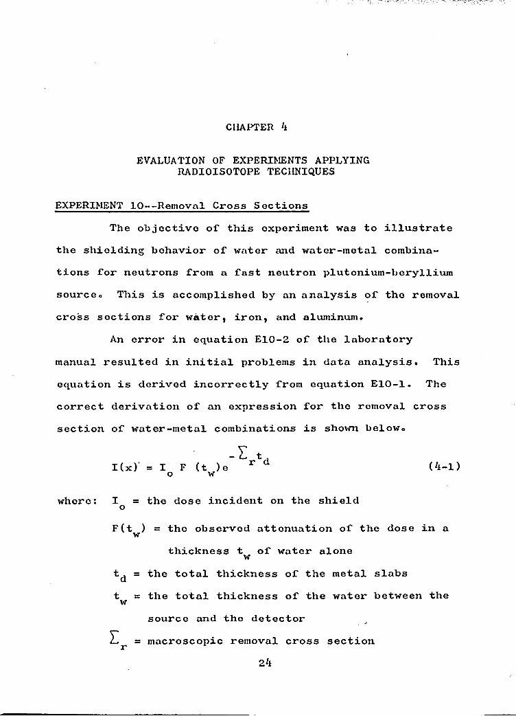
EXPERIMENT 10— Removal Cross SectionsThe objective of this experiment was to illustrate

the shielding behavior of water and water-metal combina­tions for neutrons from a fast neutron plutonium-beryllium sourceo This is accomplished by an analysis of the removal cross sections for water, iron, and aluminum.

An error in equation E10-2 of the laboratory manual resulted in initial problems in data analysis. This equation is derived incorrectly from equation E10-1. The correct derivation of an expression for the removal cross section of water-metal combinations is shown belowo

where:

I(x)

I = o

F<V

td ■t =W

-T.rtd (4-1)

the dose incident on the shield

= the observed attenuation of the dose in athickness t of water alone w

the total thickness of the metal slabsthe total thickness of the water between thesource and the detector

l . macroscopic removal cross section24

and- Z r tF(t ) = e w

w w (4-2)

Therefore,

" Z r tI (x ) = I \ eo

w w -Er*d (4-3)

where: £ = removal cross section of water only

I(x) ~ -zr *w -Zr*(jw(4-4)

= ln ITxTj ‘ r-wtw (4-5)

and\TUT, -Ir \

(4-6)

Using equation 4-6, derived above, in place of equation E10-2 in the manual, yielded removal cross sections that agree fairly well with those presented on page 188 of Valente (See Reference 13) and shown in Table 4-1.

Therefore, based upon a chi squared analysis, the value of removal cross sections determined for water, iron, and aluminum can be expected to be within the statistical distribution 90, 96, and 92 percent of the time, respec­tively =

26Table 4-1

Comparison of Observed and Expected Removal Cross Sections

Item Expected Observed 2%

Water 0.150 cm™1

-1

0.1880.162

-1cm-1cm-1

0.019

Iron 0.170 cm 0.1900.185

cm-1cm

0=003

Aluminum 0,080 cm™1 0.1050.092

—1cm-1cm

0.010

When placing the metal slabs over the source, a slight change in slab geometry would have affected the results achieved* This possible error can be corrected by construction of two channels perpendicular to the bottom of the tub into which the metal slabs would fit tightly.

To prevent streaming, the arrangement of the lead bricks at the bottom of the tub should be changed as shown in Figure 4-1.

EXPERIMENT 11— Chemical SeparationThis experiment was designed to demonstrate solvent

extraction, a useful method of chemical separation of radiotracers and of the use of tracers in chemical analysis. Ions of copper and iron were initially dissolved in

27

Figure *t.l o Revised Lead Brick Arrangement

sulfuric acid and iso-butyl alcohol was used as the extracting solution.

Some difficulties were encountered in obtaining correct extractions with the procedure outlined on page 124 of the laboratory manual. The selection of H^SO^ as the acidifying agent may have been a poor choice since according to Morrison and Freiser (See Reference 10) the sulfate tends to interfere with the extraction process.The mutual solubility of iso-butyl alcohol and water was too high for a good system.

A revised procedure for this experiment is given in Appendix B to this evaluation.

The use of ASgO^ in addition to CuSO^ and Fe(NH^)^ (S04)2 should aid in illustrating the basic chemistry. For

example, extraction of As(III) with ethyl ether should reach 68 percent while extraction of As(III) with benzene should reach 9^ percent. On the other hand, extraction of As(V) with ethyl ether should reach only 2-4 percent.

EXPERIMENT 12--Absorption of Beta ParticlesOne of the identifying characteristics of beta

radiation is its range and one of the more widely used experimental methods to determine this range was developed by Feather (See Reference 4). Feather's method compares the absorption curve of the particles whose range is to be determined with the absorption curve of a well-known standard.

This experiment uses Feather's method to determine60 234the range of the beta particles from Co and Pa when

210compared to Bi . The energies of the beta particles are determined from the relationships of Katz and Penfold (See Reference 9)• These relationships are presented on page 127 of Volume II of this thesis.

60 O O ZiExperimentally determined ranges for Co and Pa Jas well as expected ranges are shown in Table 4-2©

Therefore, based upon a chi squared analysis, the 60 234ranges observed for Co and Pa can be expected to be

within the statistical distribution 75 and 1 percent of the time, respectively•

28

29Table 4-2

Comparison of Observed and Expected Beta Ranges

Isotope Observed Expected 2X

O 0 0 82.7 mg/cm^ 280 mg/cm 0.1080.9 mg/cm^

Pa234 1015 mg/cm2 21105 mg/cm 8.7OIO65 mg/cm1'

(Experimentally determined energies for Co ;o ^and234Pa J as well as expected energies are shown in Table 4-30

Table 4-3Comparison of Observed and Expected Beta Energies

Isotope Observed Expected 2X

Co60 0.315 Mov 0.310 Mev 0.000090.312 MevPa234 2.11 Mev 2 <>32 Mev 0.0312.15 Mev

Therefore, based upon a chi squared analysis, the6o 234energies observed for Co and Pa can be expected to be

within the statistical distribution 99 and 85 percent of the time, respectivelye

30234As can be seen the results obtained for Pa were

not as accurate as those obtained for C o ^ . This was dueto the excessive extrapolation required on the Feather plot

234for Pa J . This can be remedied if a beta emitter with an234energy closer to Pa were used as the standard. Use of

32 as the standard would give additional Feather plot data points and serve to reduce the excessive extrapolation required.

A point of confusion stemmed from stop 3 in the "Results and Presentation of Data" section. This step

6o 234required that the absorption curves of Co and Pa be210normalized to the initial point of Bi • It was not clear

from the wording that the requirement was to normalize eachcurve separatelyo Then the initial points of the normalizedcurves should be made to coincide with the initial point of

210the Bi curve. A rewording of this step will avoid some possible confusiono

EXPERIMENT 13— Decontamination of SurfacesContamination results from a transfer of material

that would often be inconsequential except for its radioactivity• Such things as loss of a gas, evaporation of liquid, liquid transfer, manipulation of a solid, and absorption on surfaces all may lead to contamination•

The purpose of this experiment was to study thecorrect procedures used in the decontamination of surfaces

31It is important in a course of this type that the students thoroughly understand correct decontamination procedures o Future individual experimental research may be seriously affected by improper application of these principles.

To illustrate decontamination procedure, surfaces of glass, glazed and unglazed brick, painted and unpainted wood, asphalt tile, sheet iron, stainless steel, linoleum and plastic were tagged with radioisotopes of Na, Fe, and Cu. The students were then required to use the procedures outlined in Table 4-4 of Overman and Clark (See Reference 11) to decontaminate these surfaces.

This experiment was quite successful and illus­trated the importance associated with a knowledge of correct decontamination procedures.

CHAPTER 5

SUMMARY AND RECOMMENDATIONS

SummaryThe field of nuclear engineering is developing

rapidlyo Paralleling this development, there has been a corresponding growth in the amounts and level of research being conducted in the fieldo

The manual presented in Volume II was designed to provide a beginning nuclear engineering student with a scries of basic experiments© These experiments, if successfully completed and adequately reported, would serve as a base upon which effective, individual research could be conducted© They would also serve to illustrate some of the basic concepts necessary to a successful mastery of this highly complex and widely diversified field of study.

Based upon the results of a series of fourteen experiments conducted by each of twelve students, it is apparent that this manual does achieve the objectives for which it was designed. The effectiveness of the manual in meeting these objectives can be further enhanced if the corrections as indicated in Chapters 2, 3, and 4 in Volume I are adopted ©

32

33Recommendations

1. The manual presented in Volume XI should be revised as indicated in Chapters 2, 3» and 4 and Appendices A and B of Volume X.

2o Part I of the manual should be expanded to include a chapter on radiochemistry.

3 o Part II of the manual should be expanded to include a wider choice of experiments. Some suggested experiments are:a. The use of liquid scintillation detectors, b o Determination of neutron age.c. Evaluation of Compton scattering cross-sections od. A study of isotopes present in the air by a

method of activation analysis.4o Finally^ it is recommended that experiments using

a subcritical assembly be included in this course and that these experiments be added to the manual presented in Volume II. These experiments should include:a. Determination of cadmium ratios, b o Measurement of the diffusion coefficient•Co Determination of geometric buckling, d o Measurement of the thermal utilization factoro

e. Determination of reflector savings.

34Inclusion of these experiments will make the manual useful for both beginning and advanced laboratorycourses

APPENDIX A

ERRATA SHEET TO VOLUME II

lo Page 2, line 23 as reads, "radiation monitoring, instruments" should road, "radiation monitoring instruments."

2o Page 8, line 6 as reads, "photoelectric is shown" should read, "photoelectric effect is shown*"

3 • Page 28, line 19 as reads, "dead-time" should read, "resolving time,"

4. Page 36, line 4 as reads, "P^ = 0 .210" should read,"Pj = 0 =210."

5• Page 4l, equation 4-13 as reads, "C^" should read,"CT ="

6= Page 54, lines 31 11, 12, l4, and l6 as read, "dead- time" should read, "resolving time."

7* Page 38, line 23 as reads, "dead-time" should read, "resolving time."

8. Page 59, line 1 as reads, "dead-time" should read, "resolving time."

9. Page 63, line 15 as reads, "Aluminum, iron, and lead" should read, "Aluminum and iron."

10. Page 65, line 13 as reads, "Repeat steps 7 and 8" should read, "Repeat step 7•"

35

11. Page 65> eliminate line l4.12. Page 651 line l6 as reads, "step 6" should read,

"step 5 e1113• Page 65j line 22 as reads, "steps 7-10" should read,

"steps 6-8."l40 Page 76, line 2 as reads, "reactions" should read,

"reaction."15• Page 76, eliminate line 10ol6o Page 771 eliminate lines 21 and 22.17• Page 79» eliminate lines 1 and 2.18. Page 79, line 4 as reads, "steps 10 through 13" should

read, "steps 10 and 11."19• Page 791 line 8 as reads, "steps 10 through 13" should

read, "steps 10 and 11."20. Page 791 eliminate lines l6 and 17«21. Page 83, eliminate line 4 and renumber steps 4-13 as

36

3-12.22. Page 83, line l4 as reads, "Problem 3" should read,

"Problem 6."23 o Page 84, line 3 change step l4 to step 13 and then

add step 3 from page 83 as step l4 on page 84.24. Page 84, eliminate lines 12 and 13.25o Page 971 line 8 as reads, "A /A , " should read,S S-tfl *

26« Page 113> Figure E9-3• There should be added and tg on the curve at midway points of the increments o

27• Page 113» line 11 as reads, "Chapter 2" should read, "Chapter 1."

28. Page 118, equation E10-2 as reads,

37

- E^wat ^wat-met

should read,

" Eid . E, tTTxTi rw w

29. Page 121, last line as reads, "Valenti" should read,"Valente 11

APPENDIX B

REVISED PROCEDURE FOR EXPERIMENT 11

Procedure1. Irradiate 55 milligrams of As^O^, Oc2 gram of Fe

(NII ) (SO^) » and 1 gram of CuSO^ to provide 20 Ic of arsenic, 14 p-c of iron, and 25 ^c of copper.

2. Dissolve the As^O^ with 20 ml of 2 N NaOII. Insure that no powder remains.

3o Add 25 ml of 12 N MCI to the As^O^-NaOH solution.4. Into each of 4 graduated cylinders, marked 1-4,

transfer 1 ml of As^O^ solution.5 ° Add 5 drops of H^O to cylinders 1 and 3.6. Add 5 drops of II O to cylinders 2 and 4.7* Fill cylinders 1-4 to 2 ml with 12 N HC1.8 . Add 2 ml of benzene to cylinders 1 and 2.9• Add 2 ml of ethyl ether to cylinders 3 and 4.10. Agitate cylinders 1-4 several times for 20 seconds

each.11. Remove 1 ml each of the aqueous and organic solution.

Mark the vials containing the aqueous solution A-D and the vials containing the organic solution E-H.

12. Count each vial and record results.13• Wash all glassware.

14. Mix the CuSO/t with 20 ml of 12 N HC1.15« Into each of 2 graduated cylinderst marked 1 and 2,

transfer 1 ml of CuSO^ solution.16. Add 5 drops of 10 percent hydroxylamine hydrochloride

to cylinder lo17• Add 5 drops of H^O^ to cylinder 2 o18. Fill cylinders 1 and 2 to 2 ml with 12 N HC1.19o Add 2 ml of methyl amyl ketone to cylinders 1 and 2.20. Agitate cylinders 1 and 2 several times for 20

seconds«21. Remove 1 ml each of the aqueous and organic solution®

Mark the vials containing the aqueous solution A and D and the vials containing the organic solution C andD.

22® Count each vial.23• Wash all glassware.24® Repeat steps 14-23 with Fe(NH^)^SO^)2 in place of

CuSO^e

39

REFERENCES

1. Dlatz, Hanson, Introduction to Radiological HealthtMcGraw-Hill book Company Inc., New York, 1964, Chapter 7 °

2. Dearnaley, G., and D . Co Northrop $ S emiconductorCounters for Nuclear Radiations * John Wiley Inc*, New York, 1963•

3 o Evans, Ro D *, The Atomic Nucleus, McGraw-Hill Book Company Inc o, New York, 1955•

kc Feather, N ., Proceedings of the Cambridge Philosoph­ical Society, Vol» 34, p. 599 (193#)*

5• Flagg, John F ., Chemical Processing of Reactor Fuels, Academic Press, New York and London, 1961, Chapter4*

6. Glower, Donald D*, Experimental Reactor Analysis and Radiation Measurements, McGraw-Hill Book Company Inc *, New York, 1965•

7* Goldstein, Herbert, Fundamental Aspects of Reactor Shielding, Addison-Wesley Publishing Company, Reading, Massachusetts, 1959, pp• 367-369 •

8. Hoag, J . Barton, Nuclear Reactor Experiments, D . VanNostrand Company Inco, Princeton, New Jersey, 1958.

9* Katz, Lo and A. S. Ponfold, Reviews of Modern Physics, Vol. 24, p„ 28 (1952).10* Morrison, G . II. and II. Freiser, Solvent Extraction in

Analytical Chemistry, John Wiley Inc*, New York, 1957*

11• Overman, Ralph To, and H * Mo Clark, Radioisotope Techniques, McGraw-Hill Book Company Inc., New York, 1964.

12. Price, William Jo, Nuclear Radiation Detection, 2nded., McGraw-Hill Book Company Inc., New York, 1964.

13* Valente, Frank A., A_ Manual of Experiments in Reactor Physics, The Macmillan Company, New York, 1963•

40

Volk, William, Applied Statistics for Engineers, McGraw-Hill Book Company Inc., New York, 1958•

Yagoda, Herman, Radioactive Measurements with Nuclear Emulsions, John Wiley Inc., New York, 1949°

EXPERIMENTAL

NUCLEAR

ENGINEERING

BY

JACK GOLDSTEIN

ANDKENNETH D. KEARNS

NUCLEAR ENGINEERING DEPARTMENT COLLEGE OF ENGINEERING UNIVERSITY OF ARIZONA TUCSON, ARIZONA

EXPERIMENTAL NUCLEAR ENGINEERING

By

Jack Goldstein and Kenneth D. Kearns

Copyright © 1965 by Jack Goldstein and Kenneth D. Kearns

TO O U R W I V E S

ii

ACKNOWLEDGMENT

The authors would like to express their sincere appreciation to

Dr. Roy G. Post, without whose guidance and assistance this manual would

not have been possible. The help of many members of the Department of

Nuclear Engineering, particularly Dr. Lynn E. Weaver, Dr. Monte V. Davis

and Dr. Morton E. Weeks, is gratefully acknowledged. Finally, apprecia­

tion is due Miss Alice Garcia and Mrs. Alice McCormick for the typing of

this manual. Their attention to detail greatly assisted in the comple­

tion of the manuscript.

JG

KDK

ill

TABLE OF CONTENTS

Introduction ......................................................... 1

Part I. Introductory Chapters

Chapter 1. Nuclear Radiation and its Interactions ............ 5

Chapter 2. Radiation Safety ..................................... 12

Chapter 3. Analysis of Errors .................................. 27

Chapter 4. Counting Statistics................................... 31

Chapter 5. Report Presentation ................................... 43

Part II. Laboratory Experiments

Experiment 1. Geiger-Muller and Proportional Counters . . . . 51

Experiment 2. Portable Surveying Instruments and GeometricalEffects on Radiation ......................... 60

Experiment 3. BF^ Neutron D e t e c t o r .............................. 68

Experiment 4. Semiconductor Detectors .......................... 74

Experiment 5. Counting Statistics................ 81

Experiment 6. Scintillation Spectrometry ..................... 85

Experiment 7. Flux Mapping by Foil Activation ................ 95

Experiment 8. Analysis of Mixtures of Radioisotopes byStripping........... 103

Experiment 9. Activation of Copper and Half-lifeDeterminations ................................. 108

Experiment 10. Removal Cross Sections .......................... 117

Experiment 11. Chemical Separation .............................. 122

iv

Experiment 12. Absorption of Beta Particles .......... . . . . 129

Experiment 13. Decontamination of Surface . . . . . . . . . . 132

Experiment 14. Autoradiography .................................. 137

v

INTRODUCTION

Experimental research is the foundation for all fields of sci­

ence and engineering. In the past, this research has led to important

new discoveries which have markedly influenced our way of life. In the

future, experimental research will continue to open new vistas of knowl­

edge and understanding that will influence the course of world events.

The importance of experimentation to new scientific discoveries

necessitates the teaching of proper experimental techniques. These tech

niques include proper design and conduct of the experiment as well as ac

curate evaluation and presentation of results.

The design of an experiment should be carefully planned to in­

sure that the experiment will measure the quantity that has been speci­

fied. If prior planning is not sufficient, a great amount of time, efr

fort, and money will be wasted to obtain results which may be accurate

but worthless. Each experiment conducted must have a specific objec­

tive. The rotating of dials or the random mixing of chemicals in the

laboratory does not constitute experimental research.

All the parameters that enter into an experiment must be care­

fully considered to insure that the manner in which the experiment is

conducted will not influence results. If an item of equipment to be

used in an experiment has design limitations, these limitations must be

known, and compensated for, if the results obtained are to be accurate.

Extreme care must be taken to insure proper selection of equipment in

1

order that measurements will be taken with sufficient accuracy and sen­

sitivity.

Once an experiment has been properly designed and conducted,

the results obtained must be objectively analyzed. Experimental re­

search that begins with a strongly biased, preconceived notion of the

outcome is not only useless, but dishonest.

Years of excellent experimental design, testing and evaluation

may be forever buried in obscurity if the results obtained are not

clearly and concisely presented. Experimental results must be presented

in a manner to make all aspects of the experiment clear to the person*

interested in the area under study.

The purpose of this manual is to introduce proper techniques of

nuclear engineering experimentation.

Although the completion of a course in modern physics is as­

sumed, the introductory chapters in Part I contain a brief review of

some of the fundamental aspects of modern physics important in nuclear

engineering experimentation. Basic radiation types, their interactions

with matter, and radioactive decay are summarized briefly.

Since safe procedures are so important in handling the radio­

active materials which will be used in all experiments, Part I also con­

tains a discussion of radiation safety. Particular emphasis is placed

on dosimetry, biological effects of radiation, allowable dose and dose

rates, radiation monitoring, instruments, procedures for handling radio­

active isotopes, and decontamination procedures.

2

3The introductory chapters also contain a discussion of possible

errors encountered in experimental research. Such errors as general un­

certainties in measurement, limitation of detection equipment, uncertain­

ties peculiar to radiation measurements, and statistical errors are con­

sidered.

A chapter devoted to report presentation concludes Part I of

this manual. There is no standardized method for preparing a laboratory

report. However, this chapter, in addition to discussing report writing

techniques, outlines the format which will be used in reporting the ex­

periments in this manual.

Part II is devoted to the individual experiments which will be

conducted during this course. All of the experiments are designed to .

provide the student with direct personal experience with proper experi­

mental techniques related to nuclear engineering. The first experiments

concentrate on the use of radiation detection equipment and have limited

experimental objectives. The latter experiments concentrate on more ad­

vanced techniques and are designed to provide basic knowledge which can

be used in individual research.

PAST I

INTRODUCTORY CHAPTERS

4

CHAPTER 1

NUCLEAR RADIATION AND ITS INTERACTIONS

Introduction

This chapter is designed to provide a brief description of nu­

clear radiation and the manner in which this radiation interacts with

matter. It is not intended to serve as a complete work on these topics,

but rather a means of assisting in the better understanding of the ex­

periments in this manual. Therefore, not every particle nor every inter

action will be discussed, but only those necessary for proper under­

standing of this course. It is assumed that the student will have com­

pleted a course in modern physics and had, or will currently be enrolled

in, an introductory course in nuclear physics. The treatment of the ma­

terial will be such that it will augment the theory sections of each of

the individual experiments.

There are three types of radiation that are of primary interest

in this course. They are charged particles, gamma or x-radiation, and

neutrons.

Charged Particles

The charged particles of interest and some of their properties

are given in Table 1-1.

In passing through matter, the alpha particle is not deflected

to a great extent by any single atom, but undergoes almost continuous

5

6

slowing down, dissipating its energy by removal of some 30,000 electrons

from atoms to form ion pairs. This large number of events, governed

Table 1-1. Charged Particles

Name Symbol Mass (amu) Charge

alpha Ct 4.003873 +2

beta 0.000549 -1

positron P+ 0.000549 +1

only by the energy of the alpha particle and the ionization energy of the

medium, means that the alpha particle is stopped at a well-defined dis­

tance, called its range. Even though there is only a slight deflection

from a single interaction, the interactions are so numerous that the

range of alpha particles is relatively short. For example, an alpha

particle can be absorbed in a thick sheet of paper, a thin sheet of alu­

minum, or a few centimeters of air.

The beta particle is an electron emitted from the nucleus of an

atom. The ionization process initiated by a beta particle is similar to

that of an alpha particle. The beta particle experiences more of a de­

flection from a single interaction than does an alpha particle, but the

interactions are not so numerous. Because the mass of the beta particle

is relatively small, it undergoes acceleration and deceleration in the

vicinity of an atom. This acceleration and deceleration causes the beta

particle to give up some of its energy in the form of electromagnetic

radiation called bremsstrahlung.

7

One of the significant characteristics of the spontaneous beta

disintegration of a nucleus is the continuous energy spectrum of the

emitted particles. Each spectrum has a definite upper energy limit,

which is characteristic of the particular beta emitting nuclide.

The range of a beta particle is defined as the minimum thick­

ness of material necessary to absorb the maximum energy beta particle of

the spectrum. Since the beta particle does experience more deflection

than the alpha particle, its range is not nearly so well-defined.

The positron is a particle equal in mass to the electron and

having an equal but opposite charge. The positron's interactions with

matter are discussed in the next section.

Gamma Rays

Gamma rays are electromagnetic radiation emitted by a nucleus

in an excited state. Each gamma emitting nuclide produces radiation of

one or more discrete energies corresponding to differences in nuclear

energy levels. The energy range of gamma rays is from about 0.01 to 10

Mev.These gamma energies may interact with matter by any of three

ways: the photoelectric effect, Compton effect, and pair production.

Each photon, interacting by one of these effects, will release an or­

bital electron or an electron-positron pair and a lower energy photon.

In the photoelectric effect, the entire energy of the gamma

photon is transferred to an orbital electron. A portion of this energy

is used in removing the electron from its orbit. The remainder is

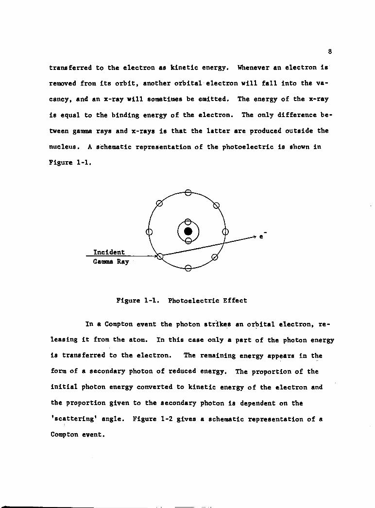
8

transferred to the electron as kinetic energy. Whenever an electron Is

removed from Its orbit, another orbital electron will fall into the va­

cancy, and an x-ray will sometimes be emitted. The energy of the x-ray

is equal to the binding energy of the electron. The only difference be­

tween gamma rays and x-rays is that the latter are produced outside the

nucleus. A schematic representation of the photoelectric is shown in

Figure 1-1.

IncidentGamma Ray

Figure 1-1. Photoelectric Effect

In a Compton event the photon strikes an orbital electron, re­

leasing it from the atom. In this case only a part of the photon energy

is transferred to the electron. The remaining energy appears in the

form of a secondary photon of reduced energy. The proportion of the

initial photon energy converted to kinetic energy of the electron and

the proportion given to the secondary photon is dependent on the

’scattering* angle. Figure 1-2 gives a schematic representation of a

Compton event.

9

Figure 1-2, Compton Event

Pair production takes place in the coulomb field of the nu­

cleus. It occurs when a gamma photon of 1.02 Mev or higher energy is

converted into an electron and a positron. Every positron ultimately

dies in an encounter with an electron, in which about 20^0* of electro-

magnetic radiation is emitted. The electron and positron are annihi­

lated producing two photons of 0.511 Mev each. These photons are called

IncidentGamma Ray

0.511 Mev

Figure 1-3. Pair Production

10

annihilation radiation. Figure 1-3 gives a schematic representation of

pair production.

Neutrons

The neutron is a neutral particle with a mass nearly equal to

that of a hydrogen nucleus. Because they are uncharged, the interac­

tions between neutrons and matter are entirely dependent upon the nu­

clear forces that exist between a neutron and the nucleus of an atom.

Since neutrons are uncharged, they cause only negligible amounts of

ionization. Therefore, neutrons travel relatively long distances in

matter when compared with charged particles. When neutrons interact

with the nucleus of an atom, the interaction may be by elastic scat­

tering, inelastic scattering, or capture.

If elastic scattering occurs, the neutron is deflected by the

nucleus with a resultant loss of kinetic energy by the neutron and gain

of kinetic energy by the nucleus. If inelastic scattering occurs, the

neutron enters the nucleus, and a neutron emerges at a different energy.

In a capture reaction, the nucleus captures the neutron and often emits

another type of radiation.

Radioactive Decay

Certain elements have radioactive isotopes which undergo spon­

taneous disintegration resulting in the emission of alpha and beta par­

ticles and the formation of a different isotope. The rate of decay of

an isotope at any time is proportional to the number of atoms present at

that time. If N0 is the number of atoms initially present, then the

number of atoms present (N) at any time (t) is given by

N = N0e"Xt (1-1)

where X represents the decay constant of the isotope under considera­

tion.

The half-life an isotope is defined as the time in­

terval over which the chance of survival of an atom is exactly one-half.

Therefore, from equation 1-1,

11

Tl/2 = (ln 2)/x (1-2)

The mean or average life (?) is given by the sum of the times

of existence of all the atoms divided by the initial number. It can be

shown that

T = 1/X (1-3)

A means of identifying an unknown isotope is by determining the

half-life or the mean life. This process will be illustrated in the ex­

periments .

CHAPTER 2

RADIATION SAFETY

Introduction

Since the beginning of the Manhattan Project in 1942, work with

nuclear radiation has involved ever increasing numbers of people.

Today, the uses of radiation have created a new industrial field. In

1942 it was realized that large numbers of relatively untrained people

would be processing enormous quantities of very active isotopes and that

adequate protective measures would have to be taken. A great amount of

research was initiated, and has continued, to determine possible harmful

effects of radiation as well as means to be used to minimize these ef­

fects. This chapter will outline the common types of radiation, quanti­

tative measures of radiation doses, possible biological effects of ra­

diation, allowable dose rates, radiation monitoring instruments, radia­

tion protection, rules for laboratory operation, and decontamination

procedures. This chapter is not intended to serve as a complete work

in the field of radiation safety, but rather as a guide to proper con­

duct in the laboratory.

Biological Effects of Radiation

Biological damage results from the destruction of cells by the

extremely concentrated or localized -deposition of energy by particulate

and electromagnetic radiation in passing through matter. In nuclear

12

13laboratory work, this damage is due basically to three types of radia­

tion: charged particles, x- or gamma radiation, and neutrons. These

types of radiation and their interactions with matter were discussed in

Chapter 1.

Although the effects of ionizing radiation on living organisms

are not completely understood, certain facts appear to be valid. Expo­

sure of living cells to radiation usually causes an undesireable change.

The amount of change in a cell is somewhat proportional to the radiation

exposure. However, at extremely low levels, such as background, this is

not always valid. Some cells, once subjected to ionizing radiation, can

be replaced by normal cells while some others cannot. Some cells, such

as those of the lymph nodes, are more susceptible to ionization than

others. For this reason, certain parts of the body, such as the hands,

are able to absorb much larger doses of radiation without harmful ef­

fects.

As well as producing an undesireable change in living cells,

radiation can sometimes produce desireable changes. Although it is

known to produce cancer, radiation is also used as a treatment for

cancer. Since cancer cells grow more rapidly than healthy cells, they

are more sensitive to radiation. Therefore, radiation has a preferen­

tial effect on cancer cells over healthy cells.

As has been discussed, the body has some recovery capability

after radiation damage, dependent on the speed of replacement of certain

body cells. For this reason, large doses incurred over short periods of

time (acute exposure) are more harmful than small doses incurred .

14

frequently (chronic exposure). If very large doses are received, large

enough numbers of cells may be affected to preclude any recovery.

Exposure to radiation can be incurred either externally or in­

ternally. Although the biological effects are the same in either case,

an internal exposure is potentially much more damaging. This increased

damage results from the fact that the irradiation is continuous until it

is eliminated from the body. Also, it is difficult to increase the

body's normal elimination rate. Radiation, taken internally, is diffi­

cult to assess quantitatively.

Radioactive materials can enter the body by ingestion, inhala­

tion, or by absorption in the skin. In considering internal exposure,

the biological half-life of the radioactive material is useful. The

biological half-life represents the time it takes for the body, by na­

tural elimination processes, to decrease the amount of the radioactive

material present by one-half. Usually it is necessary in estimating po­

tential damage to the body to consider not only the biological half-

life, but a combination of the radioactive and biological half-lives.

This combination is known as effective half-life (T) and is given by

T - %Tb + Tr (3-1)

It is easily seen from equation 3-1 that if a material has a relatively

long radioactive half-life, the importance of the biological half-life

is greatly increased.

The factors which determine the extent of radiation damage to

the body are total dose, dose rate, type of radiation, energy of radia­

tion, type of tissue involved, volume of tissue affected, and part of

body affected.

The above discussion is -intended to show the need of res­

pect for radiation and adequate protection to prevent damage by radia­

tion. The remaining portions of this chapter will elaborate on neces­

sary protective measures.

Radiation Units As Applied to Dosimetry

It would be most ideal to have a unit.of radiation-effect mea­

surement for any type of material that was the same as the reading on a

survey meter for any type of radiation. No such ideal unit exists; in­

stead, there is in present use a wide variety of terms to explain the

effects of ionizing radiation. Increased knowledge in the field of ra­

diation safety has led to the gradual development of more general radia­

tion units.

Originally the most widely known and important radioactive ma­

terial was radium. All other radioactive materials were measured by the

amount of radium present in the compound. However, when the method of

measuring the disintegration rate of a radioisotope was developed, it

was necessary to develop a unit for materials other than radium. The

'rutherford' (10^ disintegrations/second) was proposed in honor of the

prominent nuclear physicist. Lord Rutherford, but this unit has found

little usage. The 'curie', named in honor of Marie Curie, expresses the

15

rate as

16

amount of radioactive material which disintegrates at the st

one gram of radium.

Curie: 3.7 X 10 disintegrations per second,

Radiation units are used to indicate the amount of radiation

being emitted from a source or the amount of radiation being absorbed by

a certain material in a specific location. The first generally accepted

unit of radiation measurement was the roentgen.

Roentgen (r): that amount of gamma or x-radiation that willproduce one electrostatic unit (esu) of charge in one cubic centimeter of dry air at standard temperature and pressure.

It should be noted that this radiation unit deals only with gamma or x-

rays and for absorption in air. It therefore has limited usage.

As understanding developed in studying the effects of radia­

tion, the need for quantitative measurement of the energy absorbed in

biological tissue and in materials other than air became apparent. It

was also necessary to define the absorption of energy for types of ra­

diation other than gamma or x-rays. This need led to the development of

a unit known as the roentgen equivalent physical (rep).

Rep: the amount of radiation from any radiation source equiva­lent in energy dissipation to 1 r of high-voltage x-rays.

However, it was realized that the rep also had certain disadvantages.

For the same source of radiation, its absorption in various materials

varied according to the physical characteristics of the material.

17

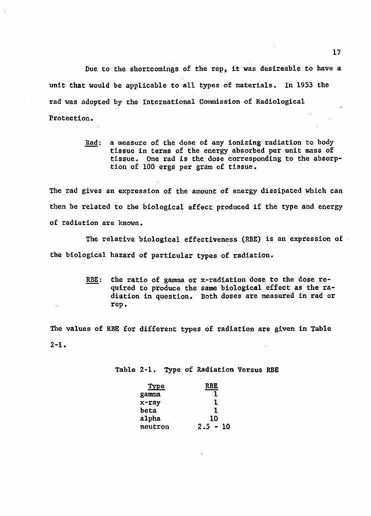
Due to the shortcomings of the rep, it was desireable to have a

unit that would be applicable to all types of materials. In 1953 the

rad was adopted by the International Commission of Radiological

Protection.

Rad: a measure of the dose of any ionizing radiation to bodytissue in terms of the energy absorbed per unit mass of tissue. One rad is the dose corresponding to the absorp­tion of 100 ergs per gram of tissue.

The rad gives an expression of the amount of energy dissipated which can

then be related to the biological effect produced if the type and energy

of radiation are known.

The relative biological effectiveness (RBE) is an expression of

the biological hazard of particular types of radiation.

RBE: the ratio of gamma or x-radiation dose to the dose re­quired to produce the same biological effect as the ra­diation in question. Both doses are measured in rad or rep.

The values of RBE for different types of radiation are given in Table

2-1.

Table 2-1. Type of Radiation Versus RBE

Type RBEgamma 1x-ray 1beta 1alpha 10neutron 2.5 -

18

The R B E for neutrons varies from 2.5 to 10 depending on the neutron

energy. The Incident number of neutrons per square centimeter equiva­

lent to one rem may be estimated from Table 2-2.

Table 2-2. Neutron Flux Dose Equivalents

N e u t r o n E n e r g y ( M e v )

Number of Neutrons Per cm2 Equivalent to a Dose of 1 rem

Thermal 0.0001 0.005 . 0.02 . 0.1 . . 0.5 . . 1.0 . .2.5 . . 5.0 . .7.5 . .10 . .

10-30 .

970 X 10* 720 X 10° 820 X 10° 400 X 10° 120 X 10° 43 X 10° 26 X 10° 29 X 10° 26 X 10° 24 X 10° 24 X 10° 14 X 10°

The most frequently used unit for expressing radiation effect

or biological dose is the roentgen equivalent mammal (rem).

Rem: a measure of the dose of any ionizing radiation to bodytissue in terms of its estimated biological effect rela­tive to a dose of one roentgen of high energy x-radia­tion.

As has been previously discussed, when any radiation passes

through matter, it loses energy in the form of ion pairs. A means of

expressing this loss of energy is by the linear energy transfer (LET).

LET: an expression of the rate at which the energy that hasbeen absorbed is used up in the system along its path length. Normally expressed as ion density per unit length of path.

19

Allowable Dose and Dose Rates

Part 20 of Title 10, Code of Federal Regulations, prescribes

maximum radiation limits. In any case where doubt may exist as to an

allowed exposure, this document should be consulted.

During any calendar quarter the whole body dose to which a

person may be exposed should not exceed 1-1/4 rems. Once this quarterly

dose level is reached, it is necessary to wait 13 weeks before an addi­

tional radiation exposure. It should be noted that the 1-1/4 rem per

quarter figure refers to the whole body dose. Quarterly allowable doses

for other parts of the body are given in Table 2-3.

Table 2-3. Maximum Allowable Quarterly Dose Rates

Allowable Quarterly DoseBody Part __________ (rem)

Whole body, head and trunk . . . . . . . . 1-1/4S k u l l ......................................... 1-1/4Eye lens ....................................... 1-1/4Pelvis .................. . . . . . . . . . 1-1/4G o n a d s ................................. 1-1/4H e a r t ..................................... 5L i v e r ......................................... 5Stomach ...................................... 5Intestines . . . . . . . . . ............... 5Bladder ....................................... 5Lungs ..........................................5Spleen ........................................ 5P a n c r e a s ................................ 5K i d n e y s .......................... 5Bone structure .............. . . . . . . . 7S k i n ........................................... 7-1/2T h y r o i d ....................................... 7-1/2Hands ........................................ 18-3/4Ankles ....................................... 18-3/4F e e t .......................................... 18-3/4

Under unusual circumstances, a quarterly allowable dose of 3

rem may be permitted. During an emergency, a one-time exposure of 25

rem may be incurred. Part 20 of Title 10 gives necessary information

relating to these exposures. It should be noted that all radiation

doses are compatible with radiation occurring from natural sources.

These sources include natural background (from cosmic radiation and na­

turally occurring terrestrial radioactive materials), displaced terres­

trial radioactive materials (such as in building or paving materials),

and man-made radiation sources (such as fallout deposits from nucleai

weapons or nearby radiation sources in storage).

At any time, the dose to the whole body, when added to the ac­

cumulated dose to the whole body, should not exceed 5(N - 18) rems,

where N is the age of the individual at his last birthday. This rule

considers that under the age of eighteen the body tissues, still in a

developmental stage, are more susceptible to radiation damage.

In many instances it will be necessary to compute the lengths

of time an individual can work within a certain proximity of a source.

The intensity of radiation from a source generally decreases with the

distance from a source. For a point source, this decrease is inversely

proportional to the square of the distance from the source. .Normally

a source can be considered as a 1point* if measurements are made one

foot or more from a source whose largest dimension is not more than four

inches. The sources used in this course will normally be considered as

point. An example will serve to illustrate the calculations.

20

21

Example 2-1: The background radiation in the laboratory is 1

mrem/hr. A source emittihg 1.5 Hev gammas is brought into the lab­

oratory. The radiation dose reading one foot from the source is

0.5 rem/hr. How many hours per week, every week, could you work ati

a distance of 10 feet from the source without exceeding your allowed

dose?

If £3 is the source strength, and R is the distance from the

source, then

0.5 100 or Sx * 0.005 rem/hr.

Therefore at 10 feet from the source, you are receiving 0.005 rem/hr

plus the background radiation of 0.001 rem/hr or a total of 0.006

rem/hr. You are allowed a whole body dose of_1.25 rem/quarter.

Therefore, you can work

(1.25)/(0.006) * 208 hours in 13 weeks

(208)/(13) * 16 hours per week.

Radiation Protection

There are three basic ways in which an individual may protect

himself from excessive external radiation exposure. These are time,

distance, and shielding. If an individual is exposed to exceedingly

high radiation levels, then care must be taken to insure that the

22

exposure does not exceed allowable limits. Accurate knowledge of the

time and amount of exposure will aid in radiation protection. Gener-.

ally, the intensity from a radioactive source decreases with increased

distance from the source. If a source must be handled, it should be

kept as far away from the body as possible. Tongs should be used to in­

crease the distance between the source and the body. If an individual

must work close to a source for a length of time that would make his ex­

posure excessive, shielding from the source should be provided. Shield­

ing can be accomplished by placing, between the person and the source, a

material which will attenuate the type of radiation being emitted to ac­

ceptable levels.

In choosing a suitable shielding material, not only the ability

of the material to attenuate should be considered, but also its cost,

and chemical and physical characteristics. Most shields are constructed

basically of either lead, steel, or concrete. For effective neutron

shielding, some material with a low atomic mass number (such as hydro­

genous materials) should be used along with a good neutron absorber,

such as boron*

Radiation Monitoring Instruments

To monitor radiation levels within a laboratory, certain ra­

diation survey devices and instruments are used. These include, but are

not limited to, film badges, pocket dosimeters, Geiger-Muller survey

meters, and portable proportional counters (Cutie Pie)♦

23

The film badge consists of a small metal "or plastic holder con­

taining one or two packets of film. One packet is sensitive to beta and

gamma radiation and the other is sensitive to neutrons. The radiation

absorbed causes a darkening of the film proportional to the amount of

radiation received.

The pocket dosimeter, a direct-reading quartz-fiber electro­

scope, is useful for monitoring where high radiation levels are ex­

pected. It has the advantage of direct reading and gives immediate in­

formation on the radiation exposure. A variation of the pocket dosi­

meter is the pocket chamber which is read on an auxiliary instrument.

These instruments are quite useful but should be used in conjunction

with a film badge which will give a permanent record of radiation expo­

sure.

T w o p o r t a b l e i n s t r u m e n t s , t h e G M c o u n t e r a n d t h e C u t i e P i e , a r e

v a l u a b l e f o r l a b o r a t o r y r a d i a t i o n s u r v e y . T h e G M c o u n t e r i s r e l a t i v e l y

a c c u r a t e f o r d e t e c t i o n o f b e t a a n d g a m m a r a d i a t i o n u p t o 2 0 m r e m / h r .

For higher radiation fields, up to 2500 mrem/hr, a Cutie Pie is more

efficient. The Cutie Pie may also be used to detect the presence of,

but not monitor for, alpha particles. For extremely high radiation

levels, specialized monitoring instruments must be used.

Rules for Laboratory Operation

A laboratory containing radioactive materials must have rules

to prevent unnecessary exposure to radiation. These rules are designed

to prevent ingestion, to minimize general radiation levels, and to

24

i n s u r e t h e p r o p e r r e t e n t i o n o f r a d i o a c t i v e m a t e r i a l s . T h e s e r u l e s a r e

a p p l i c a t i o n s o f s o u n d p e r s o n a l h y g i e n e a n d g o o d c o m m o n s e n s e .

The rules for laboratory operation are in four categories:

general procedures, handling of radioisotopes, radioactive waste dis­

posal, apd contamination.

A. General Procedurest

1« Nothing will be placed in the mouth. This prohibits smoking,

drinking, eating, and pipetting by mouth.

2. The laboratory must be kept clean and orderly at all times.

3. Personal belongings brought into the laboratory may be lost by

contamination or corrosive chemicals. " Such losses are the personal

risks of the student.

B. . Handling of Radioisotopes

1. Film badges will be worn whenever radioisotopes are, or may be,

present.

2. Pocket dosimeters will be worn whenever high radiation levels

are expected. The dosimeters afford immediate knowledge of the amount

of exposure.

3. Required radiation warning signs will be posted. (See Part 20

of Title 10, Code of Federal Regulations.)

4* All containers with radioactive materials will be clearly

tagged showing isotope, amount, and date.

5. All liquid radioisotopes must be stored in double containers.

Volatiles and dusts must be used in the hood only.

25

6. No area, without controlled access, may have a radiation level

above 5 mrem/hr. Suitable shielding and containment may be used to r e - '

duce the radiation to this level.

7. When there is a possibility of hand contamination, rubber

gloves should be worn. Any person with breaks in the skin must wear

rubber gloves.

8. Goggles, or other eye protection, must be worn when handling

hazardous chemicals.

9. At the completion of any experiment using radioisotopes, the

students, instructors, equipment, and room area must1 be surveyed for ra­

diation.

C. Waste Disposal

1. Radioactive waste, certified by the instructor to read at or

below background level, may be disposed of by placing it in a drain or

normal refuse can.

2. Radioactive waste reading above background level mist be dis­

posed of by the instructor (by controlled burial under the direction of

the University Health Physicist).

3. Liquid radioactive waste should be stored separately from solid

waste.

4. Radioactive wastes should be stored separately according to

half-life.

5. All radioactive wastes must be stored in containers which are

clearly marked.

26

D. Contamination

1. Any contamination of the body or clothing should be reported to

the laboratory instructor at once.

2. If apparatus in the laboratory is contaminated, decontamination

procedures will be undertaken to reduce the radiation level to back­

ground.

3. Under no circumstances will contaminated apparatus be returned

to its shelf position.

Decontamination

Once a piece of equipment in the laboratory or portion of the lab­

oratory itself become contaminated, proper decontamination procedures

must be undertaken. These decontamination procedures will vary de­

pending upon the type, nature, and amount of the spill. There are var­

ious methods available for decontaminating certain types of material.

Refer to Table 4-4 of Radioisotope Techniques by Overman and Clark for

specific methods of decontamination

CHAPTER 3

ANALYSIS OF ERRORS

Introduction

An experiment Is designed to answer one or more questions. It

must be designed to give these answers without influencing their out­

come, and to give answers with sufficient accuracy to define the an­

swers. In order for an experiment to accomplish all this, the experi­

menter must have adequate knowledge of the uncertainties involved in

every phase of the experiment. He must know these uncertainties in

order to analyze the data taken and determine the reliability of the

answers.

It is the purpose of this chapter to present some of the uncer­

tainties involved in nuclear engineering experimentation, and how uncer­

tainties are analyzed. It is impossible to mention all the experimental

errors which might be found; however, this chapter will give a few exam­

ple's. It is expected that detailed discussions of the errors associated

with the individual experiments will be given in the laboratory reports.

Definitions

An error in a recorded value is defined as the difference be­

tween the recorded value and the true value. Generally, errors are ex­

pressed as percentage errors or probable errors. These terms are

27

28

defined by the following equations. If x is a measured value of an

event, and T is the true value of that event, then

% error (x - T)(1Q0) T

(4-1)

Since the true value is almost never known, an expected value or best

estimate is used in its place. For example, if the average value is

taken as the best estimate to the true value, then

where

probable error in x (x - sHlOO)

x(4-2)

(4-3)

It should be noted that other means may be used to define the best esti­

mate. In the laboratory reports, the percentage error in the measure­

ment and the resulting percentage error in the final answer should both

be given.

Classification of Errors

Errors can be classified either as systematic errors or random

errors. Systematic errors are determinate errors which can be minimized

by applying known correction or calibration factors. As an example, the

efficiency of a radiation detector can be determined, and the proper

correction can be made to the recorded values. If the dead time (see

Experiment 1) of a counter is known, a suitable correction can be made

to give a more accurate count. It should be noted, however, that

29

although the correction is made, there is still some random error in­

herent in the correction itself.

Random errors are those which are accidental or indeterminate.

They can be subclassified as either gross random errors or statistical

errors. Gross random errors result from such things as contamination or

impurities in materials, both of which may cause the complete failure of

an experiment.

Statistical errors are those which result from the statistical

nature of the event. For example, in measuring the length of an object,

the exact length cannot be found no matter how accurate the measuring

device may be. The chance of the measurement being too short is as

probable as the chance of it being too long. Certain statistical dis­

tributions describe the frequency of occurrence of the long and short

measurements. These distributions and their application to nuclear

decay processes are discussed in Chapter 4.

O f t e n r a n d o m e r r o r s c a n b e r e d u c e d b y u s i n g t h e p r o p e r e q u i p ­

m e n t a n d t h e p r o p e r e x p e r i m e n t a l t e c h n i q u e . F o r e x a m p l e , i f a s a m p l e i s

c o n t a m i n a t e d , t h e s p e c t r u m ( s e e E x p e r i m e n t 6 ) c a n b e i n v e s t i g a t e d i n

o r d e r t o d e t e r m i n e w h i c h c o n t a m i n a n t s a r e p r e s e n t .

E r r o r s F r o m R a d i a t i o n D e t e c t i o n E q u i p m e n t

I m p r o p e r s e l e c t i o n o f e q u i p m e n t i s a c o m m o n m i s t a k e a l w a y s r e ­

s u l t i n g i n l a r g e e r r o r s . I n t h i s c o u r s e , h o w e v e r , t h e e q u i p m e n t s e l e c ­

t i o n h a s a l r e a d y b e e n m a d e f o r e a c h e x p e r i m e n t . S t i l l , i t i s i m p o r t a n t

30

that each piece of equipment is properly assembled and correctly used in

order to insure the success of the experiment.

Although the proper selection of the equipment is made, there

are still errors resulting from certain inherent factors in the radia­

tion detection devices themselves. It is important that the student be

aware of these errors although he may have no control over them. Some

of these inherent errors are systematic and therefore can be corrected

to some degree. Others are completely random. Electronic noise, spu­

rious counts, erratic performance of any piece of equipment, and age

variation of the equipment are all error producing factors over which

the student has no control. Care, however, must be taken to insure that

the equipment is correctly operated.

Errors From Radiation Measurements

These errors result from factors peculiar to radiation measure­

ment. Examples of factors giving rise to this type of error are absorp­

tion of radiation in detection chamber walls, self-absorption of radia­

tion, scattering and backscattering of radiation, geometrical effects,

production of secondary radiation, and absorption of radiation in air.

Often these errors can be estimated or calculated, and the recorded

values can be adjusted accordingly.

CHAPTER 4

COUNTING STATISTICS

Introduction

This chapter is intended to describe briefly the need for sta­

tistical analysis in processes associated with counting, the types of

probability distributions, and the methods of using these distributions

in laboratory procedure. This chapter is not intended to give detailed

derivations of the probability distributions, but rather to provide a

reference to the necessary equations as well as brief explanations and

examples of their use. It is expected that statistics, where appli­

cable, will be used in preparing the laboratory reports. Many refer­

ences which give the detailed theory of nuclear statistics are avail­

able. In this chapter the concern is not the uncertainties from the de­

tector, the associated equipment, or the laboratory technique, but only

the uncertainties resulting from the random nature of the relatively

small number of events in nuclear decay processes.

All nuclear and atomic events are random. However, when one

measures a macroscopic event such as the Faraday by plating silver, for20example, the large number of events, of the order of 10 , reduces the

influence of a single variation to an undetectable variation. In

counting, however, the much smaller numbers make each single variation

important.

31

32

Probability theory has a very important application in nuclear

processes because radioactive decay occurs in a random manner. Because

of this random manner, there are no true or correct values. To get the

best results, average or mean values are used. Along with this mean

value, a range around this value, within which a successive trial might

be expected to fall, is given.

A probability can be thought of as the ratio of the number of

expected successes to the number of trials. In general, we talk about

frequency distributions which describe the frequency of successes. The

following distributions have been found to be useful for nuclear pro­

cesses .

The Binomial Distribution

The binomial distribution is a frequency distribution des­

cribing yes-no type random events. It describes bivalued processes such

as flipping coins. By bivalued, it is meant that the events can take on

only two values.

If Px is the probability that an event will occur x number of

times, then

zlx xl(z-x): PX d - P)Z-X . (4-1)

where z is the number of trials, £ is the probability that the event

will occur, and (1-p) is the probability that the event will not occur.

In this case the two values are (1) that the event will occur and (2)

that the event will not occur. Because of the nature of this

33

distribution, it is obvious that x and z are confined to integers.

Equation 4-1 is the general term of the binomial expansion of (p + q)Z

where q = (1 - p ) . Therefore,

(P + q)Z - P; + + Pz.2 + ••• + P0 - (6-2)

The following example will illustrate one of the uses of the

binomial distribution.

Example 4-1: If five dice are thrown, what is the probability that

face 2 will come up on at least three dice?

The binomial distribution is applicable to this example because

throwing dice is a bivalued process in that the face 2 will either

come up or it will not. Because there are five dice, z ■* 5, and be­

cause face 2 is one of six faces on a die, p * 1/6. Since we would

like the face 2 on at least three dice, we must sum the probabili­

ties of it occurring on exactly three, exactly four, and exactly

five dice. Therefore,

5*. 250r3 " ( 1 / 6 ) ( 5 / 6 > ' - 7776- ’

P4 - T&r (I/O W - *

ps - A <i/6>5<5/6>° 7776

P - P3 + P4 + P5 7776

Therefore, if we rolled the five dice 7,776 times, we would expect

the face 2 to come up on at least three dice 276 times*

34

The binomial distribution can be used in considering the pro­

bability of radioactive disintegration, because this also is a bivalned

process. (An atom either disintegrates or it does not.) If the total

number of atoms present is H0 , the probability of x number of these

atoms decaying in a time t_ is given by

No'x x'.CN -x) 1

-Xtxx, -Xt^N0-x(1 - e ) (e (4-3)

The following example will illustrate the use of Equation 4-3.

Example 4-2: If 10 Copper 66 atoms are present initially, what is

the probability of exactly 4 atoms decaying in four minutes? The

half-life of Copper 66 is 5.2 minutes.

t - (In 2)/T1/2 X t « 0.533

e-Xt - 0.588, (1 - e~Xt) - 0.412

NQ ” 10, x ■ 4

^4 = tTgT (0.412)4(0.588)*

P4 - 0.25

The Poisson Distribution

The Poisson frequency distribution describes all random pro­

cesses whose probability of occurrence is small and constant. It is ap­

plicable to nearly all observations made in nuclear physics. This dis­

tribution is a limiting case of the binomial distribution with p « 1,

35

t h e m e a n v a l u e ( m ■ p z ) c o n s t a n t , a n d z v e r y l a r g e . T h e e q u a t i o n f o r

t h e P o i s s o n d i s t r i b u t i o n i s

Px 4e-mx ! (4-4)

Since x can only represent integers, a graph of the Poisson distribution

(Px versus x) can only be a histogram.

One very useful form of the Poisson distribution describes the

distribution in the size of time intervals between successive events of

a random process. In this case Equation 4-4 is written in terms of

time. The mean value, m, becomes equal to at where a is the average ac­

tivity (counts/time) and _t is the time. The probability Px that x

counts will not occur in a time _t is given by

Px (4-5)

More specifically, if the counter is set to shut off at a fixed number

of counts £, the probability of obtaining £ counts in a time T or less

is given by

s-1P - 1 - £ P„ (4-6)1 x-0

The following example will illustrate the use of Equation 4-6.

Example 4-3: With an average counting rate of 0.8 counts/second,

what is the probability of obtaining 4 counts in 4.5 seconds or

less?

36

a “ 0.8/sec, t * 4.5 sec, s ■ 4,

at “ 3.6

PQ - 0.027, P1 - 0.093,

P 2 “ 0.175, P4 “ 0.210

?T - 1 - (0.027 + 0.093 + 0.175 + 0.210)

PT - 0.495

The Normal Distribution

The normal frequency distribution Is an approximation to the

binomial distribution when z is very large. In the normal distribution,

the observed variable (x) is not confined to integer values but can take

on any value from -oo to +oo. The probability that a value will lie be­

tween x and x + dx is given by

(4-7)

where o’ is the standard deviation discussed in the next section of this

chapter. The probability that the mean value m is missed by an amount u

on any given trial is given by

(4-8)

Some useful calculations for Equation 4-8 are given in Table 4-1.

37Table 4-1. Calculations for Equation 4-8.

uAr 0 0.500 0.6745 1.000 1.645 2.000

*u 1 . 0.617 0.5000 0.317 0.100 0.455

From Table 4-1, it Is seen that If u “ o’, (1 - 0.317) * 0.68 or 68% of

the trials will fall within ±tr or the value of m, the true average.

Standard Deviations

For any frequency distribution, the standard deviation (cr) is

defined as the square root of the average value of the square of the in­

dividual deviations from the true value. Therefore, for a large series

of n measurements of x,

2 1“n 2crz = (1/n) E (xi - m)z (4-9)i-1

where m is the true value of what is being measured. For the distribu­

tions discussed previously, the standard deviations take the forms shown

in Table 4-2.

Table 4-2. Forms of the Standard Deviation

Distribution Standard Deviation

Binomial cr “ s M i - p )

Binomial (Form for Radioactive Decay) cr

Poisson or = x/nT

Poisson (Time Interval) <r « Vs/a

Normal cr “ cr

38

For most of the experiments in this manual, the form of the

standard deviation for radioactive disintegration will be required.

However, in many cases, X _ t will be much less than 1 thus making e

approximately equal to 1. In this case the standard deviation takes

the form of that for the Poisson distribution, <r ■ V m . This result is

expected because for the Poisson distribution p ■ (1 - e , and there­

fore the condition that £ be much less than 1 is satisfied.

In general, we will not be interested in the standard deviation

of the number of counts but rather of count rates (counts/time). If m

is the true value of the number of counts, the count rate (R) is given

by

R = m/t (4-10)

and the standard deviation of the count rate is given by

o-R = </m/t (4-11)

Because it is never possible to find the true value, a method

of estimating the standard deviations is necessary. If the number of

counts is reasonably large, m can be replaced by the number of counts

(x) . The following example will help to illustrate the method of

finding the average value and the standard deviation.

Example 4-4: Suppose we take a series of ten one-minute counts and

obtain the results shown in Table 4-3.

39

Table 4-3. Counting Series

Trial Counts/minute

1 2202 2143 1984 2045 2216 2137 2188 2089 217

10 207Total 2120

The number of counts and its standard deviation are given by

x “ 2120, (rx -V2120 - 46

x = 2120 ± 46

The average count rate and its standard deviation are given by

' R - 2120/10 ■ 212 counts/minute

<rR - V2120/10 - 4 .6

R ■ 212 ± 4 . 6 counts/minute.

This means that the probability of the true average being between

218.6 and 207.4 is approximately 68%. Suppose we had taken ten ten-

minute counts and obtained a total of 21,200 counts. The average

counting rate would then be given by

40- _ 21200 ±/21200 R " 100

R ■ 212 db 1.5 counts/minute.

Therefore by taking longer counts, we have narrowed the expected

range of the true average.

Often In the experiments In this manual, such as for a rapidly

decaying source, it will not be possible to obtain more than one count.

In these cases we consider each separate count to be an average and find

the standard deviation by taking the square root of the number of

counts. As an example, consider the decaying counts given in Table 4-4.

In plotting data, it is desirable to show the standard deviation on the

graph in order to give a better idea of the uncertainties involved.

Using the data in Table 4-4, the method of plotting is shown in

Figure 4-1.

propagation of Errors

Table 4-4. Decaying Source

Trial Counts

12345

1000 ± 32 550 ± 23 350 ± 19 280 ± 17 160 ± 13

Often it is necessary to perform some mathematical operation on

numbers with standard deviations. In these cases, we are interested in

41

Figure 4-1. Plotting Standard Deviations

the standard deviation of the result. The following equations show the

propagation of standard deviations. If r is a function of the form

r - f O ^ r ^ r g , . . . ) (4-12)

and o^, eg,... are the standard deviations of r^, ^ ,... respectively,

then the general form of the standard deviation of r is given by

" k - ai + B . 0*2 • • •

12 (4-13)

Some examples of the use of Equation 4-13 are given in Table 4-5.

MP>

42

Operation

r ■ rl ± r2

r ” rlr2/r3

r - ar1 + b

Standard Deviation

Table 4-5. Error Propagation

(fR-aei

crR ” a(r/r1)<r1

trR = X r ^

CHAPTER 5REPORT PRESENTATION

The manner in which a report is presented will, to a great ex­

tent, determine how readily experimental results are accepted. No re­

sults are meaningful until they have been communicated to other persons.

Reports should be informative, accurate, concise, technically and gram­

matically correct, readable, legible and efficiently organized. In

addition, reports should be complete enough to insure that they cover

all relevant aspects of the experiment. No necessary information should

be left to speculation or conjecture by the reader; however, unnecessary

and unrelated material should be carefully eliminated' from all reports.

The report must provide all of the information necessary for the reader

to understand and evaluate the experiment. Excess verbiage detracts and

may prevent acceptance.

Although there are many forms for laboratory reports, those

submitted in this course will conform to the minimum standards specified

in this chapter.

Laboratory reports will be required for each experiment con­

ducted. Group discussions during the laboratory period are encouraged,

but the written reports must be individual efforts. It is expected that

the literature will be searched for further information relating to each

experiment. The reports will adhere to the following format.

43

44Title Page: Include the number and name of the course, number and

title of the experiment, name of student and partners,

date performed, and date submitted (see Example 5-1).

Abstract: Give an informative but brief digest of the report, con­

veying all essential information. This section should be

complete even when separated from the rest of the report.

It should answer the question: "What is this report

about?"

Table of Contents: Indicate major subsections of the report showing

pages (see Example 5-2).

Description: Include experimental objectives and general experi­

mental method. Do not give a step by step procedure.

Include any diagrams, not presented in the manual,

which will clarify the presentation of the report.

Recorded Data: Include in tabular form both the original and re­

duced data, clearly labeled. ("Original1 does not

necessarily mean the original data sheet.)

Sample Calculations: Include typical examples of each type of non­

trivial calculation involved in the experi­

ment.

Results: Give results in both graphical and tabular form if this

enhances the clarity of the reports.

Discussion: Evaluate the results of the experiment. Discuss the

validity of the methods used and compare results with

theoretical values and/or other experimental values

45

when possible. Estimate the sources of possible errors

and their magnitude. If relevant, include the limita­

tions of the experiment and how they may be removed.

Questions and Problems: Completely answer the questions and prob­

lems indicated in each experiment.

References: List all references used in preparing the report.

Each graph must be neatly and accurately drawn and labeled.

As a minimum, all graphs will contain the title of the experiment, title

of the graph, date the experiment was performed, and the name of the

person who performed the experiment (see Example 5-3). All tables must

be labeled and presented in a manner to be easily understandable (see

Example 5-4).

NUCLEAR ENGINEERING 221

EXPERIMENTAL NUCLEAR ENGINEERING I

EXPERIMENT 1

GEIGER-MULLER AND PROPORTIONAL COUNTERS

By

John Doe

With

Jack Smith and Tom Brown

PERFORMED: OCTOBER 10, 1965

SUBMITTED: OCTOBER 24, 1965

(Example 5-1 Sample Title Page)

TABLE OF CONTENTS

DESCRIPTION OF EXPERIMENT......................... 1

RECORDED D A T A ...................................... 2

SAMPLE CALCULATIONS.................... ........... 5

RESULTS ............................................. 7

DISCUSSION ......................................... 9

QUESTIONS AND PROBLEMS ........................... 13

R E F E R E N C E S ......................................... 15

(Example 5-2. Sample Table of Contents)

(Example 5-3. Sample Graph)

EXPERIMENT 2Geometrical Effects On Radiation

Counts/minute vs BackingNovember 10, 1965

John Doe

Added Backing, mg/cm A1

4>co

49

Table 2-3. Maximum Allowable Quarterly Dose Rates

Allowable Quarterly DoseBody Part __________ (rem)

Whole body, head and trunk . . . . . . 1-1/4S k u l l ......................................... 1-1/4Eye l e n s .......................... 1-1/4P e l v i s ............................... 1-1/4Gonads .................................. 1-1/4H e a r t ................................ 5L i v e r ....................... ............... 5Stomach ..................... ............... 5Intestines .................................. 5B l a d d e r ................................ .. 5Lungs .............................. .. 5Spleen ..................... ................. 5Pancreas .................................... 5Kidneys . ..................... . . . . . . 5Bone structure . ............ ............. .. 7S k i n .............., ......................... 7-1/2T h y r o i d ........... 7-1/2H a n d s ........................................ 18-3/4Ankles .................................... • 18-3/4F e e t .......................................... 18-3/4

(Example 5-4. Sample Table)

LABORATORY EXPERIMENTS

PART II

50

EXPERIMENT 1

GEIGER-MULLER AND PROPORTIONAL COUNTERS

Purpose

The purpose of this experiment is to demonstrate the character­

istics, the operation, and the uses of the Geiger-Muller and the propor­

tional counters.

Theory

Both the Geiger-Muller (GM) counter and the proportional

counter operate on the principle of ionization of a gas. This principle

has been discussed in Chapter 1. These counters generally consist of an

anode wire enclosed by a cylinder filled with some organic gas. When a

charged particle enters the tube, it produces several ion pairs by an

ionization reaction. These ions are accelerated to their respective

electrodes by an applied electric field. They are discharged upon

reaching the electrodes, resulting in a current in the external circuit.

When the counter has detected ionizing radiation, the signal is

sent to the preamplifier (see Figure El-2). The preamplifier serves as

an impedance matching device between the detector and the non-overload­

ing amplifier.

The non-overloading amplifier and pulse height selector is a

linear pulse amplifier. It is capable of fast recovery after overload

and caq amplify small pulses in the presence of overload pulses. The

51

52

incoming signal from the preamplifier is shaped by an input network,

part of which is the coarse gain control. The signal is amplified and

then passes a fine gain control• The pulse height selector sets a

threshold for the size of the pulses.

The pulse with the desired amplitude, after leaving the non­

overloading amplifier, goes to a scaler-timer combination where the

counts are recorded.

The high voltage power supply furnishes the voltage between the

collector electrode and the cathode within the detector.

A graph of the number of ions collected versus the voltage ap­

plied across the electrodes is useful in explaining the operation of

the two counters. This graph is given in Figure El-1. In region A the

relatively weak electric field between the electrodes allows some of the

Volts

Figure El-1. Ions Collected Versus Applied Voltage

ions produced to recombine before they can be collected. As the voltage

is increased, the number of recombinations become smaller because the

ions accelerate to the electrodes faster, and have less time for "

53

recombination♦ When region B is reached, the recombination losses are

negligible, and a plateau exists* In this region all of the ion pairs

produced are collected. As the voltage is increased to region C, the

primary ions produced by the outside radiation acquire enough energy

from the electric field to produce further ionization. This phenomenon

is known as gas multiplication or gas amplification. In this region the

number of ions collected is proportional to the initial ionization. It

is in this region that the proportional counter is operated. Region C

preserves the dependence of pulse size on the primary ionization thus

making it possible to distinguish among different types of radiation.

In region D the electrons from the primary ionization reactions are ac­

celerated to the extent that the secondary ionizations are limited only

by the GM tube and the external circuit. Hence, any type of initial

ionization reaction will produce the same pulse size. In this case the

gas amplification is known as an avalanche of electrons. It is in this

region that the GM counter is operated; therefore, the GM counter pulse

size is independent of the initial ionizing reaction, thus of the nature

and energy of the radiation. Region E is the region of continuous dis­

charge and should be avoided in order to prevent damage to the GM tube.

While the avalanche is proceeding, the electrons, due to their

greater mobility, travel much faster to the anode wire than the ions are

able to move away to the cathode cylinder. As the electrons proceed to

the anode, they cause more and more ionizing reactions. Most of these

reactions occur in the vicinity of the wire. Because of their greater

mobility, the electrons are collected by the wire before the ions have

54

moved appreciably away from it* During the period that the ions are

moving to the cathode, the counter is insensitive to any outside ion­

izing radiation. This period is called the dead-time of the counter.

Upon striking the cathode, the ions may knock out other electrons thus

causing another avalanche. However, the probability of a sufficient

number of electrons being produced by this phenomenon is generally small

with organic, gas-filled tubes.

Since radiation enters the Geiger tube during the period of in­

sensitivity, the number of actual recorded counts is inaccurate. There­

fore, when any degree of accuracy is desired in the number of counts, a

positive dead-time correction is necessary*

The dead-time of most GH counters is usually on the order of

hundreds of microseconds. It should be noted that all radiation detec­

tors have inherent dead-times.

In this experiment the correct operating plateau of the GM and

proportional counters will be determined. The dead-time of the GM

counter will also be determined. Future experiments will require the

use of this information to insure that the counters are operated cor­

rectly.

Apparatus

1. Alpha source such as Polonium 210.

2. Beta sources such as Bismuth 210 and/or Cobalt 60.

3. Scaler, Baird Atomic, Model 134.

4. High voltage power supply, Baird Atomic, Model 319A.

555. Timer, Baird Atomic, Model 630.

6. Non-overloading amplifier, Baird Atomic, Model 215.

7. Fan unit, Baird Atomic, Model 1268.

8. Preamplifier, Baird Atomic, Model 231.

9. Required cables as shown in Figures El-2 and El-3.

10. Four pi windowless proportional chamber.

11. Geiger chamber, end window type.

12. Proportional gas, P-10, 90% Argon, 10% methane.

13. Geiger gas, 99.05% Helium, 0.95% isobutane.

Procedure

1. Assemble the equipment (with Geiger chamber) as shown in

Figure El-2.

2. Allow the Geiger gas to flow at a rapid rate (approximately 20

bubbles per second) through the chamber for approximately five to ten

minutes.

3. Place the Bismuth 210 beta source in the chamber near the

Geiger tube.

4. Regulate the flow of gas to approximately three bubbles per

second.

5. Slowly increase the high voltage until counts begin to appear

on the scaler.

8. Take a two-minute count.

7. Repeat step 6 at 50-volt increments. Caution: Avoid the re­

gion of continuous discharge. (Do not exceed 1700 volts.)

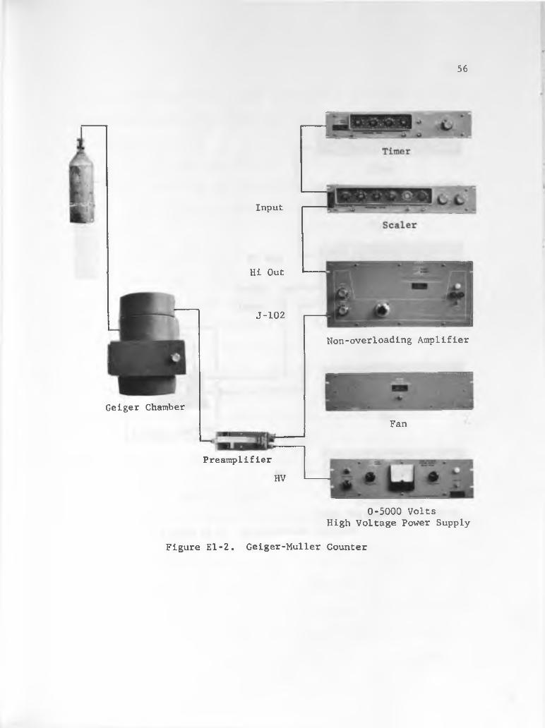
56

Geiger Chamber

Input

Hi Out

J-102

Non-overloading Amplifier

PreamplifierHV

Fan

■ ■ ■

0-5000 VoltsHigh Voltage Power Supply

Figure El-2. Geiger-Muller Counter

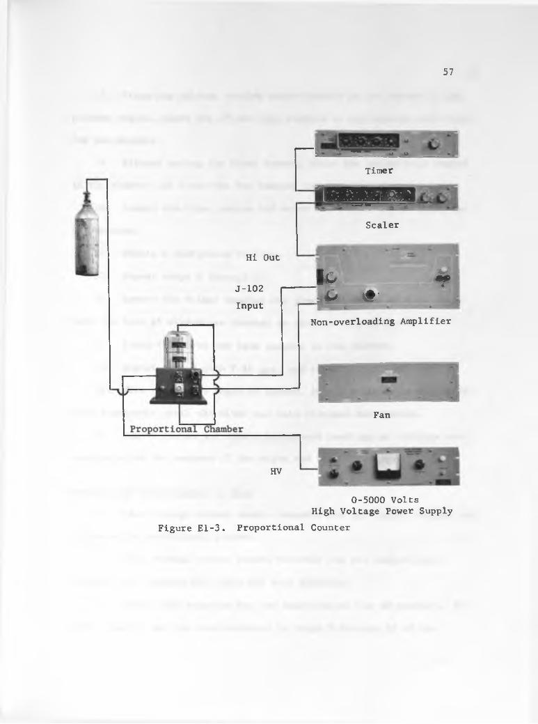
57

Hi Out

J-102Input

a* ■* v v »Timer

iHfBilhiraB--- * V. "Scaler

I - *^ -i « • ■Non-overloading Amplifier

%■

Fan

HV

0-5000 VoltsHigh Voltage Power Supply

Figure El-3. Proportional Counter

58

8. Place the voltage setting approximately in the center of the

plateau region, place one of the beta sources in the chamber, and count

for two minutes.

9. Without moving the first source, place the second beta source

in the chamber and count the two sources together for two minutes.

10. Remove the first source and count the second source alone for

two minutes.

11. Obtain a background reading.

12. Repeat steps 8 through 11.

13. Remove the Geiger chamber and preamplifier and replace these

with the four pi windowless chamber as shown in Figure El-3.

14. Place the alpha and beta sources in the chamber.

15. Repeat step 2 with P-10 gas, and repeat steps 4 and 5.

16. When the counts begin to appear, take two-minute counts at 50-

volt increments until the alpha and beta plateaus are reached.

17. Remove source and obtain background readings at voltages cor­

responding to the centers of the alpha and beta plateaus.

Results and Presentation of Data

1. Plot voltage versus counts recorded for the Geiger counter and

indicate the operational plateau.

2. Plot voltage versus counts recorded for the proportional

counter and indicate the alpha and heta plateaus.

3. Derive the equation for the dead-time of the GM counter. Use

this equation and the data recorded in steps 8 through 12 of the

procedure to calculate two values of the dead-time for the GM counter *

Find the percentage difference between these two values. Explain the

differences.

Questions and Problems

1. What constitutes background radiation?

2. Why are different gases used in the proportional counter and

the (31 counter?

3. W h y m u s t t h e c h a m b e r s b e c o n t i n u a l l y f l u s h e d ?

4. What causes continuous discharge?

5. What are the advantages and disadvantages of using the propor­

tional counters?

6. Why is quenching necessary? Describe a method by which quench­

ing is accomplished.

Selected References

Atomic Accessories, Inc., Instruction Manual, Four Pi Flow Counter Model FC110.

Hoag, J. Barton, ed., Nuclear Reactor Experiments. C. Van Nostrand Company, Inc., Princeton, New Jersey, 1958, Chapter 2.

M o n t g o m e r y , C. G . , a n d D. D. M o n t g o m e r y , T h e P h y s i c a l R e v i e w , V o l . 57, p. 1930, (1940).

Overman, Ralph T. and Herbert M. Clark, Radioisotope Techniques, McGraw- Hill Book Company, Inc., New York, 1960, Chapter 2.

Price, William, J., Nuclear Radiation Detection, McGraw-Hill Book Company, New York, 1958, Chapters 2, 5, and 6.

Stever, H. G., The Physical Review, Vol. 61, p. 38, (1942).

59

EXPERIMENT 2

PORTABLE SURVEYING INSTRUMENTS AND GEOMETRICAL EFFECTS ON RADIATION

Purpose

The purpose of this experiment is to demonstrate the character­

istics, the operation, and the uses of portable surveying instruments

and to demonstrate the effects of geometry on radiation intensity.

Theory

In principle, it is a relatively simple matter to carry out the

survey of radioactive materials or to determine the presence of radia­

tion fields. The radiation detection instruments now available provide

fairly accurate means by which this radiation is detected.

The detection of radiation, whether by portable or fixed

counter, is based on the fact that ,a charged particle or a photon pas­

sing through matter leaves along its path a string of ionized or excited

atoms which can be detected and counted (see Chapter 1).

Portable counters find their principle use in area survey re­

quirements . These requirements may include laboratory radiation checks,

civil defense radiation monitoring, and military applications for area

survey.

The Cutie Pie survey meter, which is a portable ionization

chamber, is designed to measure beta and gamma radiation of medium and

high intensity as well as to detect the presence of alpha radiation.

60

61

One outstanding feature of this meter is that it can be zeroed in an ex­

isting radiation field. This counter is shown in Figure E2-3.

The portable G M counter, shown in Figure E2-3, is a transistor­

ized survey meter designed to measure low intensity beta and gamma ra­

diation. This counter has a tendency to saturate in a strong field,

and this saturation is seen as a sharp drop in meter reading as the

source is approached. Calibration in a radiation field cannot be accu­

rately accomplished with this meter.

The portable radiation detectors provide relative radiation in­

tensities and thus have specific application in those areas previously

mentioned. If these portable detectors are to be used to their maximum

efficiency, care in operation must be exercised. The proper instruction

manuals should be consulted prior to the operation of these instruments.

The passage of gamma radiation through matter is governed

mainly by the three interactions: photoelectric effect, Compton scat­

tering, and pair production. These interactions have been discussed in

Chapter 1. The probability of a gamma photon traversing a given amount

of matter is the product of the survival probabilities for each type of

interaction. Therefore,

Ipri - Ioe”02ce"’rrxe"636 = I0e‘<ff + T + O x (E2-1)

where Ipr£ is the primary (unattenuated) radiation intensity at a dis­

tance x into the matter, I0 is radiation intensity incident on the

matter, a-, t, and e are linear attenuation coefficients for the Compton,

62

photoelectric, and pair production interactions, respectively. The

total linear attenuation coefficient is then given by

» o- + T + e (E2-2)

The attenuation of a well-collimated beam of monoenergetic

gamma photons in a 'good geometry' experiment (see Figure E2-1) is des

cribed by Equation E2-1. 'Good geometry' implies that virtually no

Compton scattered photons or annihilation photons, if pair production

is involved, reach the detector. If, however, a cylindrical shell is

placed around the source and the detector is left unshielded, the ex­

periment would have 'poor geometry* (see Figure E2-2).

Absorber

Figure E2-1. 'Good Geometry' Experiment

Absorber Source

Detector

Figure E2-2. 'Poor Geometry* Experiment

In the 'poor geometry' experiment, some of the Compton scattered and

annihilation photons are seen by the detector. Therefore, the intensity

at the detector is greater than the primary intensity. The ratio of the

63i n t e n s i t y s e e n b y t h e d e t e c t o r t o t h e p r i m a r y i n t e n s i t y i s k n o w n a s t h e

g a m m a r a y d o s e b u i l d - u p f a c t o r ( B ) .

B O b s e r v e d i n t e n s i t y P r i m a r y i n t e n s i t y

(B2-3)

A number of tables giving values for build-up factors are available.

One such table is given by Goldstein (see Selected References).

This experiment is designed to provide a familiarity with the

operation of some portable survey meters. In addition, use is made of

these meters to determine gamma ray dose build-up factors and to study

radiation intensity as a function of distance from a source.

A p p a r a t u s

1. Gamma source such as Cobalt 60 or Cesium 137.

2. Portable GM counter, Johnson, Model GSM-5.

3. Cutie Pie survey meter, Nuclear-Chicago, Model 2586.

4. Vernier caliper. Craftsman.

5. Aluminum, iron, and lead cylinder sets.

6 . M a s k i n g t a p e .

7. Lead bricks.

P r o c e d u r e

1. Make a diagram of the laboratory room.

2. Using the portable GM counter, survey the laboratory for radia­

tion levels and record on the diagram.

3. With the lead bricks, build an open-end cover and with the

masking tape, mark off a line perpendicular to the open end and lines

64

0

p M

.

1

Figure E2-3. Geiger-Muller and Cutie Pie Survey Meters

Figure E2-4. Open End Cover with Markers

6545° on either side of the perpendicular (see Figure E2-4).

4. On the masking tape, mark spaces of four inches beginning at

the face of the cover. The total length should be 20 inches.

5. Place the Cobalt 60 source in the cover and record radiation

intensities with the Cutie Pie meter at each of the points marked in

step 4.

6. Place the Cutie Pie meter eight inches from the bare Cobalt 60

source and record the intensity.

7. Place the smallest cylinder of the aluminum set around the

source and record the intensity. Repeat for each cylinder in the set.

With the vernier caliper, measure and record the thickness of each cy­

linder.

8. Repeat steps 7 and 8 with the iron set.

9. Repeat steps 7 and 8 with the lead set.

Results and Presentation of Data

1. Using the data obtained from step 6 of the procedure, plot ra­

diation intensity versus distance from the source for each line along

which the measurements were made.

2. Draw a complete diagram of the laboratory room showing the ra­

diation intensities measured during the survey. Be certain to indicate

hot spots.

3. Using the data obtained in steps 7 - 10 of the procedure, plot

intensity versus absorber thicknesses for each material on semi-log

66

graph paper. On the same graphs, plot the primary Intensity versus

thickness.

4. Considering the source to be a point, how should the radiation

intensity change with the distance from the source? Discuss how your

results compare with those expected.

5. From the graphs, find the build-up factors for |i0x ” 1. Compare

these build-up factors with those given in the appendices of Goldstein

(see references) by finding the percentage errors.

Questions and Problems

1. Which counter, the portable GM or the Cutie Pie, should be used

to survey for very low intensity beta particles? Why?

2. What are the advantages of the Cutie Pie over the portable GM

counter?

3. Discuss the proper procedure for placing the Cutie Pie into

operation.

4. Discuss the proper procedure for using the portable survey

meter to survey the laboratory.

5♦ Discuss the possible causes of the hot spots found in the lab­

oratory .

Selected References

Evans, R. D . , The Atomic Nucleus, McGraw-Hill Book Company, Inc., New York, 1955, pp. 728-735.

Goldstein, Herbert, Fundamental Aspects of Reactor Shielding, Reading, Massachusetts, 1959, pp. 367-369.

67

Nuclear Chicago Corporation, 2500 Series Cutie Pie Survey Meters, Instruction Manual, February, 1963.

William B. Johnson & Associates, Inc., Instructions, Operation and Care of Model GSM-5 Survey Meter, Montville, New Jersey.

EXPERIMENT 3

b f 3 NEUTRON DETECTOR

Purpose

The purpose of this experiment is to demonstrate the character­

istics, the operation, and the uses of the boron trifluoride (BF^)

thermal neutron counter as well as to determine the operating plateau of

the modified BFg counter.

Theory

In common with all neutral particles, neutrons can be detected

only by means of secondary charged particles which they generate in pas­

sing through matter, or by secondary processes which produce ionizing

radiation (see Chapter 1), One of the means by which these secondaryj

particles are produced is nuclear disintegration. An example of this

nuclear disintegration is the alpha particle from the B^(n,oQ reaction:

5B10 + Qn1 — > 3Li7 + 2He4 . (E3-1)

The BFg, boron trifluoride, gas-filled detector was developed

to measure thermal neutron densities. This detector employs the reac­

tion shown above to initiate the necessary gas ionization in the tube.

Subsequent multiplication of the ion pairs due to the high field gra­

dient near the anode wire results in a pulse of electrons at the anode.

68

69

Because of the very significant drop in cross section for the B10(nsa) reaction with an increase in neutron energy, the sensitivity of

this counter is very small for fast neutrons. However, if the counter

is enclosed in a neutron moderator in such a way that the neutrons are

slowed down before entering the counter, then the counter can detect

fast neutrons.

The BF3 counter, when modified to detect fast neutrons, is

known as a long counter. The conventional BF3 counter is embedded in a

cylinder of polyethylene. Around the polyethylene is a layer of cadmium

which is a very good absorber of slow neutrons but a very poor absorber

of fast neutrons.

As neutrons enter the counter, they have energies extending

from thermal up to several million electron volts. The cadmium layer

with its high thermal neutron cross section absorbs the thermal neutrons

but passes the fast neutrons into the polyethylene. As these fast neu­

trons travel through the layer of polyethylene, they are slowed to velo­

cities within the range of the detector. The neutrons at higher ener­

gies have a slightly better chance of detection than those at lower

energies, since the faster neutrons are slowed down at greater depths

in the polyethylene and have less chance of escaping before detection.

Since the BFg ionization chamber is in effect a proportional

counter, the function of the preamplifier, non-overloading amplifier,

scaler-timer, and high voltage power supply are the same as described in

Experiment 1.

70

In this experiment the operational plateau of the BFg counter

will be determined, Future experiments will require the use of the data

determined.

A p p a r a t u s

1. Neutron sources, Plutonium-Beryllium (Pu-Be) (2).

2. Scaler, Baird Atomic, Model 134.

3. Timer, Baird Atomic, Model 630.

4. High voltage power supply, Baird Atomic, Model 319A.

5. N o n - o v e r l o a d i n g a m p l i f i e r , B a i r d A t o m i c , M o d e l 215.

6. Fan unit, Baird Atomic, Model 1268.

7. Preamplifier, Baird Atomic, Model 231.

8. Required cables as shown in Figure E3-1.

9. Modified BFg counter, Reuter-Stokes, Model RSN-7A, El314.

10. Neutron howitzer.

11. Lead bricks.

12. 14 inch polyethylene plug, 4 inch polyethylene plug.

P r o c e d u r e

1. Assemble the equipment as shown in Figure R3-1.

2. Place a 14 inch polyethylene plug inside the neutron howitzer.

3. Place the two Pu-Be sources inside the howitzer on top of the

polyethylene plug.

4. Place the modified BF^ counter on top of the howitzer, sup­

porting it with lead bricks.

71

S'•»

Timer

flHHBScaler

L i ,

0-5000 VoltsHigh Voltage Power Supply

Figure E3-1. BF^ Neutron Detector

72

5. Increase the voltage slowly until the threshold voltage is

reached.

6. Increase the voltage in 50-volt increments until the opera­

tional plateau is reached. Record the number of counts at each voltage.

Caution: Do not exceed 2500 volts.

7. Reduce the voltage to threshold.

8. Place the 4 inch polyethylene plug on top of the sources and

repeat step 6.

Results and Presentation of Data

1. Plot counts recorded as a function of applied voltage, with

and without the 4 inch polyethylene plug inserted. Indicate the opera­

tional plateau.

Questions and Problems

1. What are the energies of the neutrons emitted from the sources

used in this experiment?

2. What is the absorption cross section of cadmium for these neu­

trons?

3. How are pulses resulting from reactions, other than those pro­

duced by neutrons, kept from reaching the scaler?

4. What is the cable-attenuation of the cable from the modified

BFg counter to the preamplifier? How does this affect your recorded

data?

5. Compute the thermal neutron sensitivity of the BF3 counter used in this experiment. The filling gas is 96% enriched BF^ at a pressure

73

of 20 cm of mercury. Consider a Maxwell-Boltman distribution.

6. Discuss at least two other means by which neutrons may be de­

tected.

7. What are the advantages of using the B^(n,a) reaction for slow neutron detection?

8 . What is the purpose of the holes in the front face of the poly­

ethylene in the modified BFg counter?

Selected References

Allen, W. D . , Neutron Detection, George Newnes Limited, London, 1960, Chapter 2.

Price, William J., Nuclear Radiation Detection, 2nd ed., McGraw-Hill Book Company, 1964, Chapter 10.

Reuter-Stokes Electronic Components, Inc., Boron TrifluorideProportional Counter Bulletin, No. 106, Cleveland, Ohio.

Sharpe, Jack, Nuclear Radiation Detectors, 2nd ed., John Wiley and Sons, Inc., New York, 1964, Chapter 4.

EXPERIMENT 4

S E M I C O N D U C T O R D E T E C T O R S

P u r p o s e

T h e p u r p o s e o f t h i s e x p e r i m e n t i s t o d e m o n s t r a t e t h e c h a r a c t e r ­

i s t i c s a n d o p e r a t i o n o f s e m i c o n d u c t o r d e t e c t o r s b y a n a l y z i n g a l p h a a n d

b e t a s p e c t r u m s u s i n g t h i s d e t e c t o r .

T h e o r y

O n l y i n r e c e n t y e a r s h a s t h e i m p o r t a n c e o f s e m i c o n d u c t o r d e t e c ­

t o r s t o e x p e r i m e n t a l n u c l e a r e n g i n e e r i n g b e e n f u l l y r e a l i z e d . S o f a r ,

t h e m o s t e x t e n s i v e u s e o f s e m i c o n d u c t o r d e t e c t o r s h a s b e e n f o r p a r t i c l e

s p e c t r o m e t r y . S e m i c o n d u c t o r d e t e c t o r s c a n b e u s e d t o d e t e c t t h e s a m e

t y p e s o f r a d i a t i o n a s t h e i o n i z a t i o n c h a m b e r s p r e v i o u s l y d i s c u s s e d .

H o w e v e r , t h e y p o s s e s s c e r t a i n a d v a n t a g e s o v e r a n i o n i z a t i o n c h a m b e r .

T h e p r i n c i p l e a d v a n t a g e i s t h e i m p r o v e d e f f i c i e n c y r e a l i z e d b y t h e r a p i d

c o n v e r s i o n f r o m i n c i d e n t p a r t i c l e e n e r g y t o a d e t e c t a b l e s i g n a l . A n ­

o t h e r a d v a n t a g e i s t h e s m a l l n e s s o f s i z e o f t h e d e t e c t o r .

A l t h o u g h s e m i c o n d u c t o r d e t e c t o r s p o s s e s s t h e a d v a n t a g e s l i s t e d ,

c e r t a i n i n h e r e n t d i s a d v a n t a g e s m u s t a l s o b e c o n s i d e r e d . A m o n g t h e s e

d i s a d v a n t a g e s a r e a n i n a b i l i t y t o s t o p p a r t i c l e s o f r e l a t i v e l y l o n g

r a n g e a n d s u s c e p t i b i l i t y t o n u c l e a r r a d i a t i o n d a m a g e .

W h e n a s e m i c o n d u c t o r d e t e c t o r i s u s e d t o d e t e c t n u c l e a r p a r t i ­

c l e s , e a c h o n e t h a t i s d e t e c t e d c o n t r i b u t e s t o t h e d e t e r i o r a t i o n o f t h e

74

75

detector. This radiation damage decreases charge collection efficiency.

Care must be taken to insure that radiation damage is held to an abso­

lute minimum. Unnecessary exposure to a particle emitter should be

avoided.

The semiconductor detector used in this experiment is a silicon

wafer. When a charged particle, such as an alpha or beta, enters this

silicon wafer, free electron-hole pairs are created. The rate of charge

carrier formation is nearly independent of particle energy and ioniza­

tion density. The charge carriers are moved to their respective elec­

trodes by an applied electric field. Upon reaching the electrodes, the

new charge in the circuit causes a drop in voltage across a resistor in

the external circuit.

After a particle has been detected, the resulting signal is

sent to a preamplifier which again acts as an impedance matching device

(see Figure E4-1). The signal then goes to a biased amplifier which

passes only certain amplitude pulses. Finally a scaler-timer combina­

tion is used to record the pulses.

The bias supply and noise meter provide the necessary bias vol­

tage for semiconduction detection and present a constant indication of

the noise level of the system. The ultra stable mercury pulse generator

is used as a laboratory standard to cross-calibrate pulse height analy­

zers, discriminators, and amplifiers.

Semiconductor detectors count any charged particle incident on

the sensitive surface as long as the incident angle is such that the

particle will penetrate the silicon wafer appreciably. Neutrons may be

76

detected by placing an appropriate'foil in front of the detector and

counting the reactions products. A discussion of the use of the de­

tector for gamma ray detection will be left to the student. (See the

questions and problems section of this experiment.)

This experiment will illustrate the use of a semiconductor de­

tector as a standard laboratory system. The plot of an alpha spectrum

will indicate significant properties of this detector.

A p p a r a t u s

1. Alpha source such as Polonium 210.

2. Beta source such as Carbon 14.

3. Scaler-timer, RIDL, Model 49-25.

4. I n s t r u m e n t c a s e a n d p o w e r s u p p l y , R I D L , M o d e l 29-1 (2).

5. Semiconductor detector vacuum chamber, RIDL, Model 2-10.

6. Linear amplifier, RIDL, Model 30-21.

7. N u v i s t o r p r e a m p l i f i e r , RIDL, M o d e l 31-18.

8. Bias supply and noise meter, RIDL, Model 40-14.

9. Ultra stable mercury pulse generator, R I D L , Model 47-7.

10. Semiconductor detector, ORTEC, Model NDH 025 CO.

11. Multichannel analyser such as Technical Measurement

Corporation*s Model 220.

12. Pump, Cenco, Model 90510.

13. Motor, General Electric, Model 5KH33GG106F.

14. Gage, vacuum, Cenco, Model 94030.

15. Vacuum hose, six feet.

77

16. Cables as shown In Figure E4-1.

P r o c e d u r e

1. Assemble the equipment as shown in Figure E4-1.

2. Set the two way pneumatic valve on the vacuum chamber to VAC.

Note: The two way pneumatic valve marked ATM, VAC allows venting the

chamber without turning off the vacuum pump.

3. Turn the vacuum pump on and allow it to run for one minute be­

fore taking any readings. NoteV The vacuum pump should be left running

throughout the entire experiment.

4. Take a two-minute background count.

5. Set the two way valve on the vacuum chamber to ATM.

6. Place the alpha source in the chamber on the fourth sample

holder groove from the top.

7. Set the two way pneumatic valve to VAC.

8 . A d j u s t t h e d e t e c t o r b i a s t o a l e v e l w h i c h a l l o w s m a x i m u m b i a s

c o n s i s t e n t w i t h o p t i m u m s i g n a l t o n o i s e r a t i o . N o t e : T h i s i n e f f e c t

d e t e r m i n e s t h e o p e r a t i n g p l a t e a u f o r t h i s d e t e c t o r .

9. Take a two-minute count with the chamber completely evacuated.

10. Increase the pressure in the chamber from 0 to 14.7 psi, taking

a one-minute count at each increase of 1 psi*

11. Remove the alpha source and repeat steps 4 through 10 using a

beta source.

12. Repeat steps 4 through 10 using an alpha source placed on the

bottom of the detector tray assembly.

78Input Pulser

Preamplifiero E

Linear Amplifier Mercury Pulse Generator

Bias Supply

Vacuum Chamber

Multichannel Analyzer

Scaler-TimerFigure E4-1. Semiconductor Detector

79

13. Repeat steps 4 through 10 using a beta source placed on the •

bottom of the detector tray assembly.

14. Record all counts as a function of pressure.

15. Monitor steps 10 through 13 with a multichannel analyzer by re­

cording counts per minute as a function of channel number.

Results and Presentation of Data

1. Plot counts per minute as a function of pressure for each of

steps 10 through 13 of the procedure.

2. Plot counts per minute as a function of channel number for

steps 10 and 11 of the procedure.

3. Referring to the alpha spectrum, discuss the reason why the en­

ergy of the alpha particle rises to a peak and then drops sharply.

4. In looking at the graph of alpha particles detected versus

pressure, it is seen that the number of counts per minute as a function

of vacuum chamber pressure decreases rapidly. Why does this happen?

5. In step 4 above, why is the decrease less pronounced for beta

particles?

Questions and Problems

1. Why is the semiconductor detector inefficient for use as a

gamma ray detector?

2. What is the approximate energy loss of a particle in the forma­

tion of an ion pair in the semiconductor detector? How does this com­

pare with the approximate energy loss in the formation of an ion pair

in the proportional counter?

3. Discuss the semiconductor detector's energy resolution (FWHM)

compared to a gas detector and a scintillation detector.

4. What are the purposes, characteristics, and operation of the

following items of equipment used in this experiment?

a. Ultra stable mercury pulse generator

b. Bias supply and noise meter

c. Linear amplifier

d. Vacuum chamber

S e l e c t e d R e f e r e n c e s

Deamaley, G., and D. C. Northrop, Semiconductor Counters for Nuclear Radiations, John Wiley, Inc., New York, 1963.

Goulding, Fred S., "Semiconductor Detectors— Their Properties and Applications” , Nucleonics, Vol. 22, No. 5, (May, 1964).

Oak Ridge Technical Enterprises Corporation, Instruction Manual for Surface Barrier Detectors, Oak Ridge, 1961.

Price, William J., Nuclear Radiation Detection, 2nd ed., McGraw-Hill Book Company, New York, 1964, Chapter 8 .

EXPERIMENT 5

C O U N T I N G S T A T I S T I C S

Purpose

The purpose of this experiment is to study the counting statis­

tics discussed in Chapter 4 by directly applying the Poisson, the

Poisson time interval, and the normal distributions to experimental re­

sults .

Theory

The theory supporting this experiment was discussed in Chapter

4, Counting Statistics. Additional information needed in this experi­

ment will be brought out in the results section of the experiment.

Apparatus

1. GM chamber and associated equipment assembled as shown in

Figure El-2.

2. Beta source such as Bismuth 210.

3. Aluminum absorber set. Atomic Accessories, Inc.

Procedure

1. Using the beta source: and the procedure from Experiment 1 find

the plateau region of the GM counter.

2. With the aluminum absorbers, adjust the count rate to approxi­

mately one count/second.

81

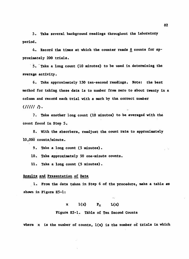
82

3. Take several background readings throughout the laboratory

period.

4. Record the times at which the counter reads counts for ap­

proximately 200 trials.

5. Take a long count (10 minutes) to be used in determining the

average activity.

6. Take approximately 150 ten-second readings. Note: the best

method for taking these data is to number from zero to about twenty in a

column and record each trial with a mark by the correct number

<///// /)•7. Take another long count (10 minutes) to be averaged with the

count found in Step 5.

8 . With the absorbers, readjust the count rate to approximately

10,000 counts/minute.

9. Take a long count (5 minutes).

10. Take approximately 50 one-minute counts.

11. Take a long count (5 minutes).

Results and Presentation of D a t a

1. From the data taken in Step 6 of the procedure, make a table as

shown in Figure E5-1:

x l(x) Px L(x)

Figure E5-1. Table of Ten Second Counts

where x is the number of counts, l(x) is the number of trials in which

x counts were recorded, Px is given by Equation 4-4 (a is found from

Steps 5 and 7), and L(x) ■ nPx where n is the total number of trials.

2. Plot a histogram of l(x) and L(x) versus x.

3. Plot Pu , experimental and theoretical, versus x.

--Poisson Time Interval

4. From Steps 5 and 7 of the procedure, calculate the average ac­

tivity.

5. Calculate at for each reading taken in Step 4.

6 . Find the fraction of values of at which are less than 2, 4,

6, 8, 10, and 12. (This gives the experimental values of P% in Equation

4-6.)

7. Calculate the theoretical values of Pg, P4 , Pg, Pg, F^q , and

using Equation 4-6 and compare these with the experimental values

found in Problem 3.

8 . Calculate the average t for 8 counts both experimentally,__ nt = x/( £ tj/n), and theoretically, t * s/a, and compare.1—1

9. Calculate the standard deviation in this average time.

--Poisson

10. Discuss the differences between l(x) and L(x) given above.

11. From Steps 9 and 11 of the procedure, determine :m.

12. Calculate the experimental standard deviation (Equation 4-9)

and the theoretical standard deviation (o'theo. = V™) • Compare these

values.

--Normal

13. Find the experimental values of Pu by counting the fraction of

83

84

trials (Step 10) which fall outside (a) m + 0.5creXp, (b) m ± 1 •0o'exp,

(c) m ± l.Sffgjjp, and (d) m ± 2 .0(rexp.

14. Calculate Pu (Equation 4-8 and Table 4-1) for the values shown

in a, b, c, and d above.

15. Discuss the differences in the curves of the experimental and

theoretical values of P^.

16. What differences in the experimental curve of Pu would there

have been if you had counted the fraction of trials below m - 0 .5

and above m + 0 ♦5crexp, etc., separately?

Questions and Problems

1. From Equations 4r7 arid 4-8 show that for “ “ 1, Pu * 0.317.2. From Equation 4-1 and the conditions of the Poisson distribu­

tion, derive Equation 4-4.

Selected References

Evans, Robley D., The Atomic Nucleus. McGraw-Hill Book Company, Inc., New York, 1955, Chapters 26 and 27.

Friedlander, Gerhart, and J. W. Kennedy, Nuclear and Radiochemistry, John Wiley and Sons, Inc., New York, 1955, Chapter 9.

Volk, William, Applied Statistics for Engineers, McGraw-Hill Book Company, Inc., New York, 1958.

Wilks, S. S ., Elementary Statistical Analysis. Princeton University Press, Princeton, New Jersey, 1948.

Youden, W. J., Experimentation and Measurement, National Science Association, Washington, D. C., 1962.

EXPERIMENT 6

S C I N T I L L A T I O N S P E C T R O M E T R Y

P u r p o s e

T h e p u r p o s e o f t h i s e x p e r i m e n t i s t o s t u d y s c i n t i l l a t i o n s p e c ­

t r o m e t r y b y a n a l y z i n g k n o w n a n d u n k n o w n g a m m a r a y s p e c t r a .

T h e o r y

S c i n t i l l a t i o n d e t e c t i o n i s b a s e d o n t h e f a c t t h a t a c e r t a i n

c l a s s o f s u b s t a n c e s , u s u a l l y r e f e r r e d t o a s p h o s p h o r s , e m i t l i g h t a s a

r e s u l t o f i n t e r a c t i o n s w i t h r a d i a t i o n . T h i s l i g h t e m i s s i o n i s c a u s e d b y

t h e f l u o r e s c e n t n a t u r e o f t h e m a t e r i a l . T h e t e r m p h o s p h o r , a l t h o u g h

g e n e r a l l y u s e d , i s a m i s n o m e r b e c a u s e m o s t s c i n t i l l a t i o n c r y s t a l s u s e d

t o d a y a r e f l u o r e s c e n t , a n d n o t p h o s p h o r e s c e n t , m a t e r i a l s . W h e n a

c h a r g e d p a r t i c l e e n t e r s t h e f l u o r e s c e n t c r y s t a l ( t h e p h o s p h o r ) , i t g i v e s

u p i t s e n e r g y i n e x c i t i n g a n d i o n i z i n g t h e a t o m s o r m o l e c u l e s . T h e e x ­

c i t e d a t o m s t h e n r e t u r n t o t h e i r u n e x c i t e d s t a t e s b y g i v i n g u p t h e i r e x ­

c i t a t i o n e n e r g y a s p h o t o n s . T h e i n t e n s i t y o f t h e l i g h t e m i t t e d f r o m t h e

p h o s p h o r i s u s u a l l y d i r e c t l y p r o p o r t i o n a l t o t h e a m o u n t o f e n e r g y g i v e n

u p b y t h e i n c i d e n t p a r t i c l e . W h e n u n c h a r g e d g a m m a r a y s e n t e r t h e p h o s ­

p h o r , t h e l i g h t p h o t o n s a r e p r o d u c e d b y t h e s e c o n d a r y p a r t i c l e s r e ? *

s u i t i n g f r o m t h e i n t e r a c t i o n s o f g a m m a r a d i a t i o n w i t h m a t t e r . I n t h i s

c a s e , a l s o , t h e i n t e n s i t y o f t h e e m i t t e d l i g h t i s p r o p o r t i o n a l t o t h e

e n e r g y a b s o r b e d . S c i n t i l l a t i o n s p e c t r o m e t r y i s b a s e d o n t h i s

85

86

proportionality. Using scintillation spectrometry it is possible to

identify the energies of the incident radiation. In this experiment we

will be concerned with the operation of a scintillation detector and the

use of this detector in analyzing a gamma ray spectrum.

As was discussed in Chapter 1, gamma photons may interact with

matter by three processes: the photoelectric effect, Compton scat­

tering, and pair production. Each photon, interacting by one of these

effects will eventually release an orbital electron of the crystal's

atoms. The electrons then undergo energy changes resulting in emission

of light.

By means of a light pipe and reflector, a large fraction of the

light photons are transmitted to the photocathode of photomultiplier

tube. To minimize losses it is necessary for the crystal to have a high

optical transparency. When the light photons strike the photocathode,

they produce photoelectrons by the photoelectric effect. These photo­

electrons are then accelerated in an electrostatic field between the ca­

thode and the first dynode (see Figure E6-1). This dynode is at a posi­

tive potential relative to the cathode. Each accelerated photoelectron

possesses enough energy to knock out several electrons from the dynode.

There may be as many as ten secondary electrons for each initial elec­

tron striking the dynode. This amplification is repeated at each dy­

node, and the electron current is amplified as the electrons are acce­

lerated from dynode to dynode. The output current at the anode may be

more than a million times as great as the current originally emitted

from the photocathode. The pulses, however, remain proportional to

87

Light LightReflector

+200 V +600 V

+100 V +300 V +500 V +700 V

FirstPhosphor Photocathode AnodeDynode

Figure E6-1. Scintillation Detector

photon intensity.

The pulses from the scintillation detector are sent to a linear

amplifier in the analyzer (see Figure E6-3). From the amplifier, the

pulses are sent to two discriminator circuits. One discriminator is set

to pass all pulses over a voltage determined by the base level control.

The other discriminator passes all pulses over a certain voltage deter­

mined by the base level and window width controls. By comparing pulses,

an anticoincidence circuit allows only a narrow band of energy to pass

to the ratemeter. The width of this narrow band of energy is adjustable

from 0 to 10 volts by the window width control.

This narrow band of energy is processed through integrating

circuitry to a counter where it is displayed as counts. Simultaneously

a scan control panel is used to display the information on a recorder.

88

In the photoelectric effect, the entire energy of the gamma photon is transferred to an orbital electron where:

E = photoelectric energy hy = energy of the incident photon w * binding energy of the electron h * Planck’s constant v = frequency in cycles per second

hvx = energy of X-ray

then,

E - hv - w + hvx (E6-1)

hvx * w (E6-2)

E ■ hv (E6-3)

In analyzing a gamma ray spectrum, the most prominent peaks

below 1.5 Mev are usually due to the photoelectric effect. Note the

photoelectric peaks in Figure E6-2. The center of the photoelectric

peak is the photoelectric energy, and this energy is proportional to

the original gamma energy.

In a Compton event, the gamma photon is scattered or deflected

by an orbital electron. Compton electrons have a range of energies de­

pendent on the scattering angle. These energies will be indicated as

a continuum increasing to a maximum below the photopeak where:

Ece " Compton edge, or maximum energy of the Compton electron.

then.

89

Ece hv1 + .511

2hv(B6-4)

The Compton continuum and peaks are shown in Figure E6-2.

With a crystal of normal size (1" to 3"), some gamma rays will

pass through the crystal, and a proportion of these will be reflected

into the crystal at reduced energies. These photons will be added to

others that are scattered near 180° within the crystal to produce a

hackscatter peak. This peak is shown in Figure E6-2. Therefore, where:

E^g = hackscatter peak energy

then.

Ebs h v _ 1 + 2hy

.511(E6-5)

Pair production occurs when a gamma photon of 1.02 Mev or

higher energy is converted into an electron and a positron. The elec­

tron and positron are annihilated producing two photons with energies of

0.511 Mev. There is a high probability that the two scintillations will

be seen by the phototube as one flash of double intensity. When both

annihilation photons escape the crystal, a pair production peak will

occur at 1.02 Mev below the photopeak. Therefore, where:

then.

Ea *» resultant energy where both annihilation photons escape the crystal

Backscatter Peak

Photoelectric Peak Photoelectric Peak

Compton Edge

Compton Continuum

Figure E6-2. Cobalt 60 Gamma Ray Spectrum VOo

91

Ea ■ hv - 2m0c2 (E6-6)

If one of the annihilation photons strikes an electron within the re­

solving time of the crystal, the equivalent photon energy will be added

to show a peak at 0.511 Mev below the photopeak. Therefore, where:

Ey - resultant energy where one annihilation photon escapes the crystal

then,

Eb = hv - myC2 (E6-7)

If both annihilation photons are absorbed in the crystal, the total en­

ergy will show at the photopeak. These peaks are shown in Figure E6-2.

A spectrogram is a graphic record of the total of all effects

in the scintillation crystal indicated as counts per time for each en­

ergy. Each photoelectric peak will have a corresponding Compton effect

pattern, and if the energy level is high enough, pair production peaks.

In this experiment unknown isotopes will be determined from

analysis of their gamma ray spectra. Gamma ray spectrometry has wide

application in experimental nuclear engineering and will be further il­

lustrated in Experiment 8 .

Apparatus

1. Gamma source such Cobalt 60.

2. TWo unknown gamma sources.

3. Recording spectrometer. Nuclear-Chicago, Model 1820A.

4. Recorder, Bristol, Model 1FH560-51.

5. Scintillation detector. Nuclear-Chicago, Model 1421.

Procedure

1. Assemble the equipment as shown in Figure E6-3. Note: the in­

structor will have allowed a one-hour warm-up for the radiation ana­

lyzer.

2. Place the Cobalt 60 source in the scintillation detector.

3. Follow the instructions outlined in the instruction manual for

calibration and initial adjustments of the recording spectrometer.

4. Run a gamma spectrum with the Cobalt 60 source.

5. Run gamma spectrums for the two unknown sources.

Results and Presentation of Data

1. Plot the gamma spectrum from the Cobalt 60 source on semi-loga­

rithmic graph paper. Identify the photoelectric peaks, pair production

peak, Compton edge, Compton continuum, backscatterrpeak, and annihila­

tion radiation peaks.

2. Plot a calibration curve (energy versus base line) from the

above data on linear paper. Note: measure the base; line in half-inches

from the start of the tape.

3. Plot the two unknown gamma spectrums on semi-logarithmic graph

paper. Identify all peaks as in 1, above.

4. From the calibration curve, determine the gamma energies of the

unknown sources and from this identify these sources. Justify your de­

cision.

92

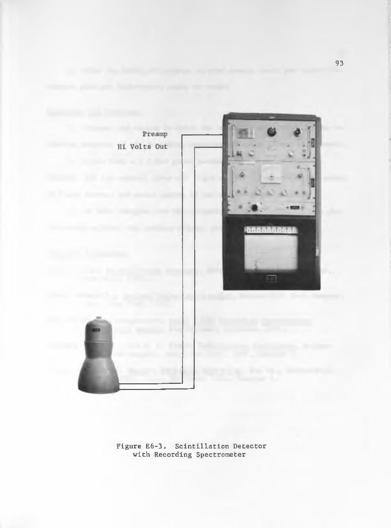
93

Figure E6-3 . Scintillation Detector with Recording Spectrometer

94

5. With the Cobalt 60 source, at what energy would you expect the

Compton edge and backscatter peaks to occur?

Questions and Problems

1. Discuss the manner in which the window width setting on the ra­

diation analyzer of the recording spectrometer would affect your result.

2. Given that a 1.2 Mev gamma photon enters a scintillationo

crystal, and the crystal gives off light at 4500 A, determine the number

of light photons per gamma photon if the system is 75% efficient.

3. At what energies are the following effects dominant: the pho­

toelectric effect, the Compton effect, and pair production?

Selected References

Birks, J. B., Scintillation Counters, McGraw-Hill Book Company, Inc., New York, 1953.

Chase, Robert L . , Nuclear Pulse Spectrometry, McGraw-Hill Book Company, Inc., New York, 1961.

Nuclear-Chicago Corporation, Model 1820B Recording Spectrometer Instruction Manual, Des Plaines, Illinois, 1961.

Overman, Ralph T., and H. M. Clark, Radioisotope:Techniques, McGraw- Hill Book Company, Inc., New York, 1960, Chapter 2.

Price, William J., Nuclear Radiation Detection. 2nd ed., McGraw-Hill Book Company, Inc., New York, 1964, Chapter 7.

EXPERIMENT 7

FLUX MAPPING BY FOIL ACTIVATION

Purpose

The purpose of this experiment is to illustrate the method of

foil activation in determining a neutron flux distribution.

Theory

A standard method of measuring neutron flux is that of foil ac­

tivation. This method Is based on the fact that certain stable iso­

topes, upon capturing a neutron, are transformed into radioactive iso­

topes. The resulting activity can be counted by standard methods and

related to the neutron flux.

If ora represents the microscopic absorption cross section, V

the volume, and N the number of nuclei per cubic centimeter of the

foil, then the activity (A) produced by the neutron capture in the

foil is given by

A - 0N<raV(l - e‘Xt) (E7-1)

where 0 is the neutron flux at the foil, \ is the decay constant of

the radioisotope resulting from the neutron capture, and t is the ex­

posure time of the foil. If • p is the density and A the atomic

weight of the foil, N0 is Avogadro*s Number, then N is given by

95

96

(E7-2)

The product of the number of nuclei per cubic centimeter and the micro­

scopic cross section is known as the macroscopic cross section (2).

S a e (E7-3)

Therefore Equation E7-1 becomes

A - 0 2 aV(l - e"Xt) (E7-4)

If the exposure time is long compared to the mean life of the

radioactive isotope, then

(E7-5)

where A g is the saturation activity. The saturation activity is the

maximum activity that a foil can attain from a given neutron flux.

Therefore, from equations E7-4 and E7-5,

As m —i

A ____■ e-Xt (E7-6)

It is evident that if A, X , and V are known, the flux can be

found from Equation E7-5.

By the use of cadmium sandwiches placed around the foils, it is

also possible to determine the thermal neutron flux. Recalling from

Experiment 3 that cadmium absorbs almost all thermal neutrons, it is

seen that only neutrons above about 0.4 ev will reach the foil in the sandwich. Clearly, if A g_ ^ represents the activity induced by thermal

neutrons ( 0 . 4 ev) and.As„fa8t: represents the fast neutron flux

( 0 . 4 ev), then

97

Dividing Equation E7-7

A s-th = Ag ™ ; A s-fast

by A s-fast 8ives

— - i + As -.th A s-fast A s-fast

(E7-7)

(E7-8)

A s/Ag_£a8t. is defined as the cadmium ratio (R^^) and is a measurement of

the degree of thermalization of neutrons.

In finding the thermal flux, the quantity A g / A g , ^ is of in­

terest. This quantity is known as the cadmium ratio correction and is

defined by

kcr = 1 ' l/*cd

Therefore the thermal flux is given by

_ As-th kcrAs 0th ” Z a V 2 a V

(E7-9)

(E7-10)

In order to determine 0 ^ , the quantities which must be measured are A s

and Ag_j=ag f If Gy and Cc are the count rates observed for the bare and

cadmium covered foils respectively, we have

0% = KyAg(l - e-Xt), and (E7-11)

Cc = ^cA s-fast(^ ” e ) (E7-12)

98

where t is the irradiation time and Ky and Kp are constants of propor­

tionality which account for the decay of the foils before and during

counting, as well as for various efficiency factors. For a foil, K is

given by

K « KjK^KQKpK^KgKgKf (E7-13)

where:

-XTKj = e = correction for decay between end of irradiation and beginning of count (T ■ elapsed time),

1 -K = — --- ■ = correction for decay during counting (t = dura-d tion of count),

Kq * correction to zero bias for the counting system,

Ke = correction for counter efficiency, including geometry factor (use 60% in this experiment),

K ° 1 - CTjj * correction for dead time of counter (C * count rate, td * dead time),

Kg = self-shielding factor.

Kg ■ backscatter correction factor,

Kf = flux depression factor for the foil.

Each of the above factors should be carefully considered; however, in

some cases, certain of these corrections are not required. Since the

foils are very thin, the self-shielding and backscatter corrections are

99

negligible (i.e., Kg - Kg ” 1). The factor Kq accounts for the loss of

pulses resulting from the bias discrimination against noise. The method

of finding Kq will be indicated in the procedure section of this experi­

ment. Kg accounts for the flux depression of the neutron distribution

in the foil due to absorption of neutrons by the foil. For this experi­

ment Kg is assumed to be 0.85.

From Equations E7-11 and E7-12 we have

A = <B 7 -U >

and

A =-fast ■ -jr ! _Cg-\t (E7-15)

Therefore from Equations E7-14 and E7-15 and from the definition of the

cadmium ratio given earlier, we have

KcCbRcd " <E7-16>

In order to obtain accurate results, it will also be necessary

to normalize the weights of the foils.

In this experiment a method of foil activation to determine

neutron flux will be used. The correction factors necessary to obtain

accurate fluxes will also be illustrated. Foil activation is a commonly

used technique in many areas of experimental nuclear research, and this

experiment will provide a basis for further individual work using this

method.

Apparatus100

1. GM counter and associated equipment as shown in Figure El-2.2. Neutron howitzer.

3. Polyethylene inserts marked 1 through 6 .

4. Polyethylene plugs (2), 4 inches and 14 inches.

5. Plutonium-Beryllium sources (2) .

6 . Indium foils marked 1 through 12.

7. Cadmium sandwiches (6).

8. Analytical balance, Mettler, Number 61569.

Procedure1. Assemble equipment as shown in Figure El-2.

2. Weigh the indium foils.

3. Tape the indium foils on the polyethylene inserts at the red

lines. Tape foil one to insert one, etc.

4. Place the inserts into the holes corresponding to the numbers

on the inserts.

5. Place the 4 inch polyethylene plug in the howitzer, place the

Pu-Be sources on top of this plug, and place the 14 inch plug on top of

the sources. Record the time of insertion of the sources.6 . Irradiate the foils for 5 hours.

7. Remove the foils simultaneously and record the time of removal.

8 . Allow the foils to decay for ten minutes prior to counting.

9. Using two of the foils, determine the dead-time of the GM

counter.

10. Using one of the foils, record counts versus bias voltage

101

setting (Pulse Height Selector) from 10 volts to 80 volts In Increments

of ten.

11. Count each of the foils for two minutes. Record the time at

the start of each count and the number of the foil being counted.

12. Place the remaining indium foils into the cadmium sandwiches.13. Repeat steps 3, 4, 5, 6, 7, 8, and 11.

Results and Presentation of Data

1. Plot counts versus bias voltage from data taken in Step 10 of

the procedure.

2. Plot thermal neutron flux versus distance from the source.

3. Plot RC(} and kcr versus distance from the source.

4. Plot the total neutron flux versus distance from the source.

5. Normalize the weights of the foils and calculate A s from

Equation E7-11 for each of the six positions. Calculate 0 for each

position using Equation E7-5. (Note: V * m/p).

6 . Calculate K c .

7. Calculate Rc<j» kcr, and 0 for each position.

8 . From the bias voltage curve, calculate Kq by taking the ratio

of the counts at the bias voltage used to the counts at zero bias vol­

tage (extrapolated).

9. Calculate Ky from Equation E7-13.

Questions and Problems

1. Indicate the nuclear reaction involved in this experiment and

the appropriate decay scheme.

102

2. What properties of indium make it appropriate for use in foil

measurements? List several other foil materials and discuss the proper­

ties which make them useful.

3. Should the cadmium ratio be higher or lower at the source rel­

ative to its value at the edge? Why?

4. Derive the equation Kg = (1 - e~^'t) A t .

Selected References

Hoag, J. Barton, Nuclear Reactor Experiments. D. Van Nostrand Company, Inc., Princeton, New Jersey, 1958, pp. 10-14.

Hughes, Donald J., and R. B. Schwartz, "Neutron Cross Sections", U S A E C Report, BNL-325 (2nd ed.), 1958.

Price, William J ., Nuclear Radiation Detection, 2nd ed., McGraw-Hill Book Company, New York, 1964, pp. 336-342.

Valente, Prank A. (ed.), A Manual of Experiments in Reactor Physics, The Macmillan.Company, New York, 1963, pp. 58-70.

EXPERIMENT 8

ANALYSIS OF MIXTURES OF RADIOISOTOPES BY STRIPPING

Purpose

The purpose of this experiment is to demonstrate stripping, a

method of separating the spectrum of a single radioactive isotope from

the complex spectrum of a mixture of radioisotopes.

Theory

The methods of scintillation detection and analysis of gamma

ray spectra have been discussed in previous experiments. The knowledge

gained from these experiments will now be used to analyze mixtures of

radioisotopes. This type of analysis has valuable application in the

field of nuclear engineering as well as many other scientific disci­

plines .

The type of analysis used in this experiment is stripping.

Stripping is accomplished by the subtraction of gamma ray spectra to ob­

tain a desired result. This result may be the determination of a single

isotope from a mixture of isotopes, the determination of a pure isotope

without background, or the determination of impurities in a radioiso­

tope.

A multichannel analyzer examines and sorts pulses into one of

its channels. This sorting or analysis is done on an amplitude basis.

Data display and various readout systems provide observation and

103

104

recording of the amplitude as data accumulates or after It has accumu­

lated.

Input pulses are converted Into a digital number and stored in

a digital computer memory. Numbers from this memory unit can be dis­

played or readout by the multichannel analyzer.

In this experiment we will strip the spectra of background and

Chlorine 38 (NH^Cl) from a N a ^ C l ^ spectrum. This will be accomplished

automatically by using a multichannel analyzer. Initially a spectrum of

Sodium 24 (NagCO^) should be analyzed to ascertain critical peaks of so­

dium. Therefore, when the stripping procedure has been accomplished, it

will be possible to compare the results with the previously analyzed

Sodium 24 spectrum.

Apparatus

1. Radioactive samples of NaCl, NH^Cl, and Na^COg.

2. Cobalt 60 source for calibration.

3. Multichannel analyzer with digital recorder.

4. Scintillation detector, Baird Atomic, Model 810.

5. Non-overloading amplifier, Baird Atomic, Model 215.

6 . High voltage power supply, Baird Atomic, Model 319A.

7. Required cables as shown in Figure E8-1.

Procedure

1. Assemble the equipment as shown in Figure E8-1. (The in­

structor will demonstrate the use of the multichannel analyzer.)

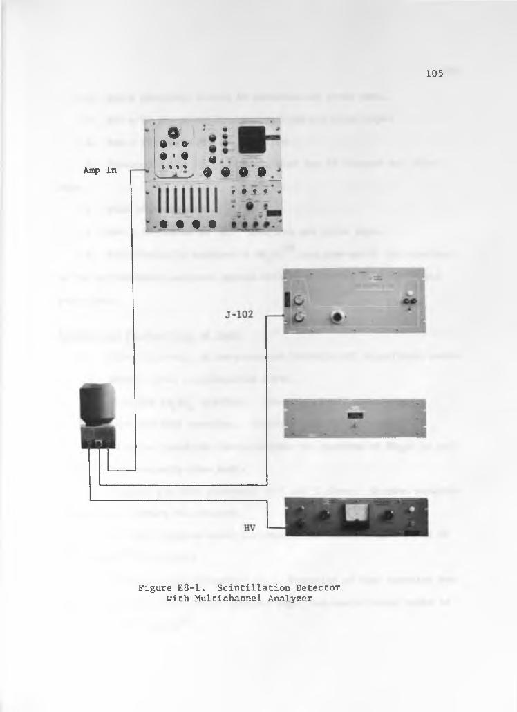
105

Amp In

a# * %# ' #$ % % %>__

• w

%# e e e

* e j *

• see

M M

Figure E8-1. Scintillation Detector with Multichannel Analyzer

106

2. Run a 10-minute Cobalt 60 spectrum and print tape.

3. Run a 10-minute background spectrum and print tape.244. Run a 10-minute Nag COg spectrum.

5. Electronically subtract background for 10 minutes and print

tape.

6 . Plot this spectrum.

7. Run a 10-minute N a ^ C l ^ spectrum and print tape.388 . Electronically subtract a NH^Cl spectrum until the spectrum

on the multichannel analyzer agrees with that plotted in 6 above and

print tape.

Results and Presentation of Data

1. Plot the Cobalt 60 spectrum and identify all significant peaks.

2. From 1, plot a calibration curve.

3. Plot the NagCOg spectrum. Identify significant peaks.

4. Plot the NaCl spectrum. Identify significant peaks.

5. Plot the resulting spectrum when the spectrum of NH^Cl is sub­

tracted electronically from NaCl.

6 . Compare the data presented in 3 and 5 above. Discuss possible

differences between the spectra.

7. At what energies would you expect the photoelectric peaks of

N a ^ and Cl^® to appear?

8 . From the data determined in 7, determine at what energies you

expect the backscatter peaks, Compton edge, and annihilation peaks to

occur for N a ^ and C l ^ \

107

Questions and Problems

1. Discuss the method of operation of the multichannel analyzer

used in this experiment. Include as a minimum the operation of signifi­

cant controls for spectrum analysis.

2. What isotopes of sodium and chlorine are irradiated to giveO Z O Q O Z O Q

Na and Cl ? What percentage of the activity of Na and Cl are by

gamma emission?

3* What type of crystal is used in this experiment? Why?

4. Draw the decay schemes of N a ^ and Cl^**.

Selected References

Overman, Ralph T. and H. H. Clark, Radioisotope Techniques. McGraw-Hill Book Company, Inc*, New York, 1960, Chapter 10.

EXPERIMENT 9ACTIVATION OF COPPER AND HALF-LIFE DETERMINATIONS

Purpose

The purpose of this experiment is to study the buildup and

decay of radioisotopes as well as elementary methods of determining

half-lives.

Theory

The relationship of the half-life of a radioisotope to nuclear

processes has been discussed in Chapter 2. The activity (disintegra­

tions/time) of a foil at a particular exposure time, t is represented

by Equation E7-4.

A - 0 2 aV(l - e-Xt) (E9-1)

Since the count rate (N) is directly proportional to the activity (A),

the ratio of two count rates for two different exposure times can be

written as

Ni 1 - e *"1N2 1 - e-kt2

(E9-2)

From Equation E9-2 and a representative buildup curve it is possible to

transcendentally solve for X and from this determine the half-life of

the radioisotope.

108

109The half-life of a radioisotope can also be determined directly

from a decay curve. If a decay curve (counts versus time) represents

only a single radioisotope, the half-life can be determined in the fol­

lowing manner:

1. Pick any count rate (N) on the decay curve,

2. Divide this by 2 (N/2),

3. The time from N to N/2 on the decay curverepresents the half-life.

However, a decay curve may represent the combined activity of

two or more radioisotopes. In this case it is necessary to separate the

complex curve into individual decay curves representative of each radio­

isotope present. If, in a complex curve, the half-lives are signifi­

cantly different, the activities are large enough, and the counting time

is long enough, the process of separating the curves is relatively .

simple. The activities of the radioisotopes with the shorter half-lives

will decay from the complex decay curve, eventually leaving only the

constant decay rate of the isotope with the longest half-life. For two

radioisotopes, the typical decay curve is given in Figure E9-1. The decay curve for the longest-lived isotope is then found by extrapo­

lating from the constant decay portion of the total curve (see Figure

E9-1)♦ The decay curve for the shorter-lived radioisotope is found by

subtracting the long-lived decay curve from the complex curve (see

Figure E9-1). The separate half-lives are then easily found by the

method described above for a single isotope.

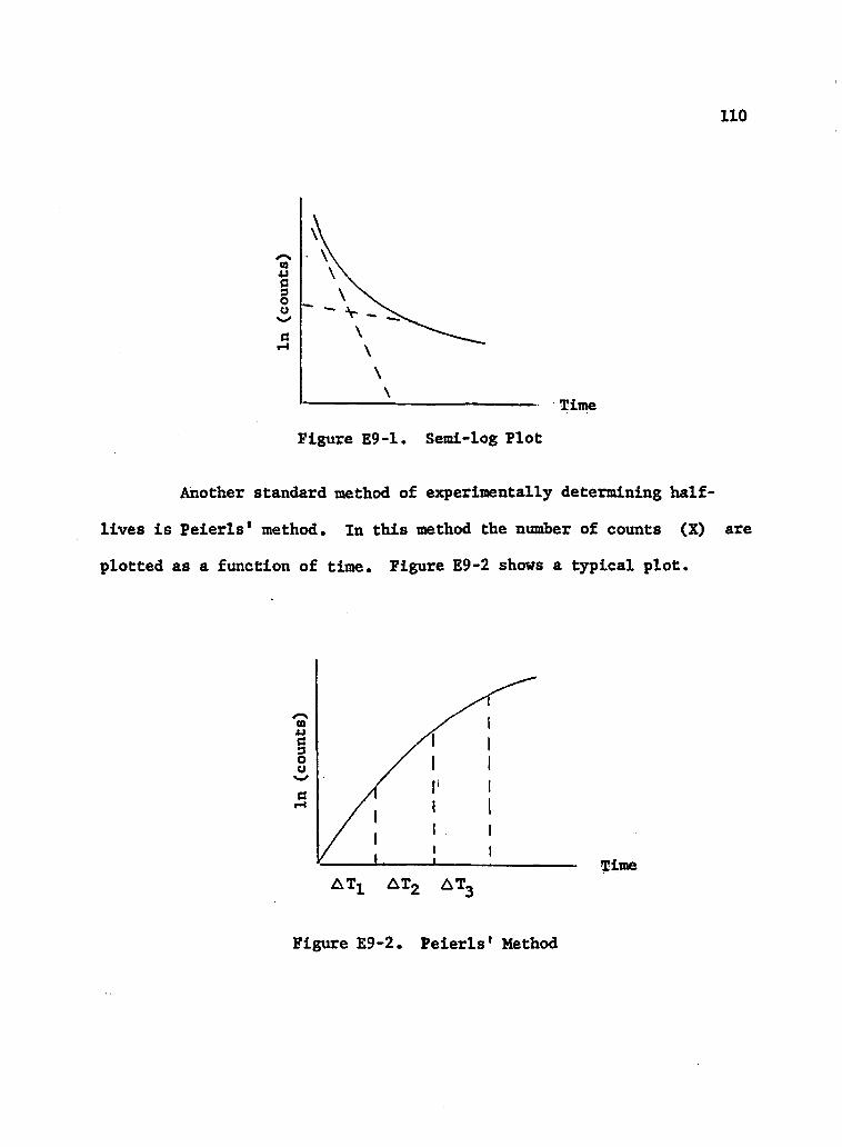
110

Figure E9-1. Semi-log Plot

Another standard method of experimentally determining half-

lives is Peierls1 method. In this method the number of counts (X) are

plotted as a function of time. Figure E9-2 shows a typical plot.

Figure E9-2. Peierls’ Method

Ill

It should be noted that Figure E9-2 does not show a buildup curve, but

rather a plot of the total counts (summed) versus time for a decaying

source. The abscissa is divided into n equal time intervals ( ATj_).

The total elapsed time is then n A T . If A represents the number of

atoms decaying in the i-th interval, then A N ^ atoms have an average

lifetime (S^) of

and for A Ng atoms.

- 1/2 A T

S2 = 1/2A T + A T « 3 / 2 A T

and so forth for S3 , 84,..., Sn . Furthermore,

A N i = A X £ - b A T

(E9-3)

(E9-4)

(E9-5)

where b is the count rate of background alone.

The total of the lifetimes of all the atoms which decay between

0 and n A T is given by

A N 2 U / 2 A T ) + A N 2(3/2AT) + A N 3(5/2AT) + ••• (E9-6)

During this time the total number of atoms whose individual lifetimes

are observed is given by

N - A N l + A N 2 + A H 3 + (E9-7)

Therefore, the average life (S) of all the observed atoms is given by

1X2

or

A Ni (1/2 A T ) + A N2(3/2 AT) + a N3(5/2a T) + ••• ANj + ANg + ANg + ••• (E9-8)

AN i + 3AN2 + 5AN3 + ••• - AT ANi + AN2 + AN3 + ••• 2 (E9-9)

The average life is related to mean life (t ) by the following equation:

S =L

nATtdN

1

n A T ,(N0/T)te /Tdt

/„n A TdN

L

n A T(N0/T)e"t/Tdt

(E9-10).

Completing the integration gives

S = T 1 -nATT

n A T / r , e - Iif T « t (E9-11)

In determining the half-life, S is found from Equation E9-9 and is

substituted into Equation E9-11. The mean life can be related to the

half-life (see Chapter 2).

The two-point method is still another means of calculating the

half-life. It uses the same type of plot shown in Figure E9-2. How­

ever, in this case, the curve is divided into two equal intervals (see

Figure E9-3). The average activity at t^ and t2 (see Figure E9-3) is

given by A N ^ / A T and A N 2/ A T , respectively, where A N ^ and A N 2 are

given by Equation E9-5. In Chapter 2 we saw that the instantaneous ac­

tivities at t^ and t2 can be related by the following equation:

113a2 ■ " tl) (E9-12)

If the relation between the Instantaneous activity and the average acti­

vity Is not dependent on time, then

a2av tl) (E9-13)

Therefore,

and, therefore.

± 2 2 = ^ 1 e-X(t2 - tl)A T A T

T t2 “ tl

In ANja n 2

(E9-14)

(E9-15)

Figure E9-3. Two-Point Method

This experiment will amplify the discussion in Chapter 2 by ac-

tually determining the half-life of Cu by four different methods. In

addition to this, the methods previously explained in Experiment 7 will

114

be used to plot a buildup curve of C u ^ and decay curves of C u ^ and

Cu66.

Apparatus

1. GM chamber and associated equipment as shown In Figure El-2,

Experiment 1.

2. Copper foils marked 1 through 6.

3. Polyethylene insert number 1.

4. Neutron howitzer.

5. Plutonium-beryllium sources (3).

Procedure

1. Assemble the equipment as shown in Figure El-2, Experiment 1.

2. Remove the foil that the instructor has irradiated for 24 hours

and count the foil by recording the counts for a 25 second time period

out of every 30 seconds. Note: this allows five seconds to record and

reset for the next count.

3. Tape copper foil number 1 to the polyethylene insert.

4. Irradiate foil number 1 for one minute.

5. Successively tape foils numbered 2 through 5 to the polyeth­

ylene insert and irradiate for 2, 5, and 10, and 20 minutes respec­

tively.

6 . Count each foil for two minutes, being certain to keep the time

from the end of irradiation to the start of counting constant for all

foils.

7. After all foils have been counted for two minutes, count the

115

foil that was Irradiated for 20 minutes, recording successive times for

200 counts. Continue this until the decay rate approaches a constant

value.

Results and Presentation of Data661. Plot buildup curves (experimental and theoretical) for Cu .

2. Plot the decay curve for the foil irradiated 20 minutes.

3. Plot the decay curve for the foil irradiated 24 hours.

4. Plot the decay curve as shown in Figures E9-2 and E9-3 for the

foil irradiated 20 minutes.

5. Determine the half-life of C u ^ by the four methods outlined in

the theory section of this experiment. How does each value compare with

the actual half-life of Cu^^?

6. From the decay curve of the foil irradiated for 24 hours, find

the half-life of Cu^^ and Cu^^. Compare these with actual values.647. Determine the relative saturation counting rates due to Cu

and C u ^ activity,

8. Calculate the relative activity of C u ^ and C u ^ from the acti­

vation cross sections and irradiation time. Does this confirm the re­

sults of Problem 7? Explain any differences.

Questions and Problems

1. From Equation E9-10, derive Equation E9-11.

2. Draw the decay schemes of Cu®^ and Cu^® and describe the

nuclear reactions involved in this experiment.

3. In the two-point method, show that the relation between the

instantaneous activity and the average activity is not dependent on

time. Hint: in Figure E9-3, compare the slope of the tangent of the

curve at t to the slope of chord connecting two points equidistant

either side of t.

Selected References

Evans, R. D., The Atomic Nucleus, McGraw-Hill Book Company, Inc.,New York, 1955, pp. 812-818.

EXPERIMENT 10REMOVAL CROSS SECTIONS

The purpose of this experiment is to study the shielding of

fast neutrons by water and several water-metal combinations.

Theory

The shielding of neutrons is actually a study of the manner in

which fast neutrons behave in matter. Normally, the shielding of neu­

trons occurs by the slowing down of fast neutrons due to elastic and

inelastic collisions and the subsequent capture of the slowed neutrons

as a result of the higher absorption cross sections at the lower ener­

gies. Because it is necessary to slow the fast neutrons, hydrogenous

materials constitute an important part of neutron shields. This experi­

ment will show that hydrogenous materials in combination with certain

metals form effective neutron shields.

One measure of the effectiveness of neutron shields is the ef­

fective removal cross section. The effective removal cross section of a

material is a cross section which describes the removal of neutrons by

any process from a beam of neutrons incident on the material. The equa­

tion that describes this removal is

I - I0e“Ertd (E10-1)

Purpose

117

118

where

I * Intensity at td

I0 == intensity incident on the shield

Er = effective removal cross section of the shield

tj = thickness of the material.

Due to the fact that the BFg counter used in this experiment

efficiently detects only slow neutrons, a water moderator will be used

in combination with layers of iron and aluminum. To measure the removal

cross section of the shield, it will be necessary to eliminate the ef­

fect of the water moderator. Therefore, the removal cross section of

the shield is determined by subtracting the effect of the water from the

overall effect of the water-metal combination. A more useful form of

Equation E10-1 is

The relaxation length (Xr) is the thickness of material which

causes a drop in intensity by a factor of e.

E lp^vat ~ lnIwat-met (E10-2)r td

(E10-3)

This experiment is designed to study the attenuation and ab­

sorption of neutrons in water and certain water-metal combinations by

the concept of removal cross sections. Removal cross sections and re­

laxation lengths for certain metals will be determined.

119

Apparatus

1. BF3 counter and associated equipment as shown in Figure E3-1,

Experiment 3.

2. Aluminum tub .

3. Mounting bracket for BF3 probe as shown in Figure E10-1.

4. Pu-Be source♦

5. Iron plates.

6 . Aluminum plates.

7. Lead bricks.

Procedure

1. Assemble the equipment as shown in Figure E3-1, Experiment 3,

and Figure E10-1, this experiment.

2. Fill the aluminum tub with water to one inch from the top.

3. Place the lead bricks in a square arrangement in the center of

the tub.

4. Place the Pu-Be source in the lead bricks.

5. Measure the activity (counts/minute) with the probe one inch

from the source.

6. Repeat this process every one inch until the count rate becomes

negligible.

7. Repeat Steps 5 and 6 with 2, 4, and 6 inches of iron over the

source.

8 . Repeat Steps 5 and 6 with 2, 4, and 6 inches of aluminum over

the source.

120

Figure E10-1. Experimental Arrangement for Removal Cross Sections

121

R e s u l t s a n d P r e s e n t a t i o n o f D a t a

1. Plot on the same graph the normalized count rate versus dis­

tance from the source for water and for each water-aluminum combination.

(Use semi-log graph paper.)

2. Plot on the same graph the normalized count rate versus dis­

tance from the source for water and for each water-iron combination.

3. Calculate the removal cross sections of water, iron, and alu­

minum by calculating the values at several different distances from the

source and averaging the results.

4. C a l c u l a t e t h e r e l a x a t i o n o f l e n g t h s o f w a t e r , i r o n , a n d a l u ­

m i n u m .

Questions and Problems

1. Why should the removal cross section not be calculated from the

data taken near the source?

2. Discuss in detail the reasons why the curves of the water-metal

combinations have values greater than those of just the water alone.

3. If a stronger source is used, what modifications would have to

be made to the experimental setup? Explain.

S e l e c t e d R e f e r e n c e s

Goldstein, Herbert, Fundamental Aspects of Reactor Shielding. Addison- Wesley Publishing Company, Inc., Reading, Massachusetts, Chapter 6 .

Valenti, Frank A., A Manual of Experiments in Reactor Physics, The Macmillan Company, New York, pp. 177-188.

EXPERIMENT 11CHEMICAL SEPARATION

The purpose of this experiment Is to separate a metallic Ion by

solvent extraction and determine distribution coefficients by measuring

the activities of the resulting aqueous solutions and alcohol extrac­

tions .

Theory

The processes of radiochemical separation have important appli­

cations in the field of nuclear engineering. Basically, the methods

used to separate radioactive substances are the same standard methods

used to separate non-radioactive substances. These methods include, but

are not limited to, precipitation, ion exchange, filter paper chromatog­

raphy, and solvent extraction. This experiment will be concerned with

solvent extraction.

Solvent extraction is a method by which one or more extractable

solutes are separated by their preferential solubility in an immiscible

extracting solvent. The extent to which a given solute partitions can

be expressed in terms of a distribution coefficient (extraction coeffi­

cient), k d .

When the two phases are at equilibrium (rates of transfer in

both directions are equal), the distribution coefficient is given by

Purpose

122

123

Kjj - C2/CL (Ell-1)

where and Cg represent the concentration of the solute In the two

solvents. If the solute Is a radioactive substance, the concentration

in each phase is directly proportional to the activity of each phase.

Therefore, the distribution coefficient can be expressed as the ratio of

the activities,

K d - A 2/A^ (Ell-2)

This ratio gives an easy method of determining Kp. Therefore, the

amount of solute that has been extracted can be readily measured.

In this experiment we will extract ions of copper and iron,

measure their activity, and determine distribution coefficients. The

ions will initially be dissolved in sulfuric acid and the extracting so­

lution will be iso-butyl alcohol.

Apparatus

1. Scintillation detector and associated equipment assembled as

shown in Figure E7-1, Experiment 7.

2. Following chemicals:

Sulfuric acid, I^SO^, 1 N

Potassium thiocynate, KSCN, 0.5 N

Copper sulfate, CuSO^

Ferrous ammonium sulfate, Fe(NH^)g(SO^)g

Iso-butyl alcohol

Hydrogen peroxide, H 2O2

124

3. Bottles, 8 ounces (2)

4. Graduated cylinders, 10 ml (28)

5. Volumetric pipettes, 1 ml (2)

6 . Volumetric pipettes, 2 ml (2)

7. Droppers (20)

8 . Plastic vials (16)

Procedure

1. Irradiate 1 gram each of GtiSO^ and Fe(NH^)2(SO^)2 «

2 . Mix each irradiated salt with 100 ml of 1 H

3. Pour 10 ml of each mixed solution into separate graduated cyl­

inders .

4. Into each of four graduated cylinders, marked 1 - 4 , transfer

one ml of Fe(NH^)g^SO^)2 solution. Use one ml volumetric pipette for

the transfer.

5. Into cylinders 2 and 4, put 5 drops of H 202 .

6 . Into cylinders 3 and 4, add 0.5 ml of 0.5 H KSCN.

7. Fill graduated cylinders 1 - 4 to two ml using 1 N H 2S0^.

8 . Using a two ml volumetric pipette, add two ml of iso-butyl al­

cohol to cylinders 1 - 4 .

9. Place polyethylene stoppers on cylinders and agitate suffi­

ciently to cause solvent extraction.

10. Remove one ml each of the aqueous and extracted solution, using

droppers to decant and graduated cylinders to measure. Mark the , : ■

graduated cylinders containing aqueous solution A-D and the graduated

cylinders containing extracted solutions E-H.

11. Transfer the contents of A-H into plastic vials marked A-H.

12. Count each vial for two minutes.

13. Wash all glassware used in Steps 4 - 1 0 .

14. Repeat Step 4 using CuSO^ solution in place of Fe(NH^)gCSO/p2

solution.

15. Repeat Steps 5 - 1 3 .

Results and Presentation of Data

1. Calculate the distribution coefficient for each extraction

system. Be sure to include with these coefficients, a description of#|-|- , | I, t

the ions which were extracted in each case (i.e., Fe , Fe , etc.)

Questions and Problems

1. Describe the nuclear reactions involved in this experiment.

Sketch the decay schemes of the radioisotopes.

2. Show that it is unnecessary to correct for the differences in

the times between irradiation and counting. Is a correction necessary

to account for the short half-life of C u ?

3. Write the chemical equations describing the processes taking

place in each of the eight cylinders before the iso-butyl alcohol is

125

added

126

Selected References

Flagg, John F ., Chemical Processing of Reactor Fuels, Academic Press, New .York and London, 1961, Chapter 4.

Overman, Ralph T. and H. M, Clark, Radioisotope Techniques, McGraw-Hill Book Company, Inc., New York, 1960, Chapter 9.

EXPERIMENT 12ABSORPTION OF BETA PARTICLES

The purpose of this experiment is to study the absorption of

beta particles in matter.

Theory

One of the identifying characteristics of beta radiation is its

range. The range of a beta particle is generally defined as the minimum

thickness of material necessary to absorb the most energetic beta par­

ticle of the particular spectrum under consideration. Since each beta

emitting isotope has a characteristic beta spectrum, it also has a char­

acteristic beta range.

The results of many experiments have shown that there is a def­

inite range-energy relationship. Katz and Penfold (see selected refer­

ences) have proposed the following empirical relations:

R0(mg/cm2) - 412 En , n * 1.265 - 0.0954 In E (E12-1)

0.01 Mev < E < ~ 3 Mev

R0(mg/cm2) = 530 E - 106, Mev < E < ~ 2 0 Mev (E12-2)

In the above equations, R@ is the range and E is the maximum energy of

the beta spectrum under consideration.

Purpose

127

128

One of the more widely used experimental methods to determine

the range of beta particles was developed by Feather (see selected ref­

erences) . Feather*s method compares the absorption curves of the parti­

cles whose range is to be determined with the absorption curve of a

well-known standard.

To determine an unknown range by Feather*s method, absorption

measurements (counts versus absorber thicknesses) are made for the known

and unknown isotope (i.e., the isotope with the unknown range). From

these measurements the instrument and ganana backgrounds are subtracted.

The resulting pure beta absorption curves are then plotted after they

have been normalized to the same initial point (see Figure E12-1). The

known range of the standard is then divided into N equal parts, T%,

Tg,... T^, and the fractional beta transmissions are found for each T^.

The thicknesses of the absorber giving the same fractional transmissions

are then found for the unknown isotope by horizontal lines shown in

Figure E12-1. These thicknesses are labeled T^, T^,* * * T^. Each of

Absorber Thickness (mg/cnr)

Figure E12-1. Pure Beta Absorption Curves

129

these thicknesses are multiplied by N/i, and the resulting products are

then plotted against i. This plot is known as a Feather plot. To de­

termine the unknown range, the Feather plot is extrapolated to i * N,

and the unknown range is taken from the extrapolated point. (See Figure

E12-2.)

\\\ extrapolated

1 . 2 3 4 .i

N

Figure E12-2. Feather Plot

In this experiment the ranges and energies of several beta

emitting isotopes will be found by Feather's method. These ranges will210be compared with generally accepted values. Bi , with a range of

o508 mg/cm , will be used as the standard.

Apparatus

1. GM counter assembled as shown in Figure El-2.

2. Aluminum absorber set. Atomic Accessories.

3. B i ^ ® , P a ^ ^ , and Co**® beta sources.

130Procedure

1. Place the Bi source in the chamber and count for one minute.

2. Place a small aluminum absorber between the source and the de­

tector and count for one minute.

3. Repeat Step 2 with increasing absorber thicknesses until the

count rate is reduced essentially to background.

4. Repeat steps 1 through 3 for the other beta sources.

5. Estimate and record the thicknesses of the GH chamber window

and the air between the window and the source.

Results and Presentation of Data

1. Plot counts versus absorber thickness for each source. Note:

the thicknesses of the GH window and the air between the source and the

window must be included in the thickness of the absorber.

2. Graphically subtract gamma and instrument backgrounds from the

absorption curves. (This gives the pure beta absorption curves.)

3. Normalize each of the pure absorption curves to the initial

point of the B i ^ ® curve and plot the P a ^ 4 an<j co60 each with the B i ^ ®

curve.

4. Determine the ranges of the P a ^ ^ and the Co**® sources using

Feather's method and compare these ranges with accepted values. (Use

N = 10.)

5. Determine the beta energies of the isotopes and compare these

with accepted values.

210

131Q u e s t i o n s a n d P r o b l e m s

1« Would the accuracy of Feather's method be Increased by making

N > 10? Explain.

2. L i s t s e v e r a l i s o t o p e s w h i c h w o u l d m a k e g o o d s t a n d a r d s . G i v e

t h e i r e n e r g i e s a n d r a n g e s . W h a t m a k e s t h e m g o o d s t a n d a r d s ?

3. H o w d o e s b a c k s c a t t e r i n g a f f e c t t h e r e s u l t s o f t h i s e x p e r i m e n t ?

4. Using equations E12-1 and E12-2, plot R0 versus beta energy

(0.01 Mev to 10 Mev). Use log-log graph paper.

S e l e c t e d R e f e r e n c e s

Evans, Robley D . , The Atomic Nucleus. McGraw-Hill!.Book Company, .New York, 1955, pp. 621-629.

F e a t h e r , N . , P r o c e e d i n g s o f t h e C a m b r i d g e P h i l o s o p h i c a l S o c i e t y ,Vol. 34, p. 599, (1938).

Katz, L. and A. S. Penfold, Reviews of Modern Physics, Vol. 24, p. 28, (1952).

EXPERIMENT 13DECONTAMINATION OF SURFACES

The purpose of this experiment is to study the procedures used

to decontaminate surfaces.

Theory

Radioactive contamination is the undesired presence of radioac­

tive materials in amounts that may be harmful to personnel and material.

In addition, this contamination may cause inaccurate experimental re­

sults. Contamination originates from a loss of material that would

often be inconsequential except for its radioactivity. Such things as

loss of a gas, evaporation of a liquid, liquid transfer, manipulation of

a solid, and absorption on surfaces all may lead to contamination. Sur­

face contamination is the deposition and attachment of radioactive mate­

rials to the surface, and it is the decontamination of a surface with

which this experiment is concerned.

The decontamination of a surface is a measure of the extent to

which radioisotopes can be removed from a contaminated surface. This

decontaminability is normally expressed as a decontamination factor

(DF).

DF - aCtlVlty (E13-1)final activity

Purpose

132

133Although there are many different means of decontaminating sur­

faces, certain established procedures will yield the best results. A

list of decontaminants for various surfaces is given in Table 4-4 of

Overman and Clark (see selected references).

Decontamination methods, regardless of the type of surface to

which they are applied, should concentrate on a thorough cleaning of the

surface without damaging the surface itself. If, however, noncorrosive

methods do not result in proper decontamination, then harsher treatments

should be used. For example, if it is necessary to decontaminate a piece of wood, and if normal washing does not produce the desired re­sults, it may be necessary to sand away the contaminated surface. The

basic rule is to employ a treatment that is as mild as possible but will

still decontaminate successfully. Mild reagents and extensive scrubbing

are generally successful in reducing the contamination to a desired

level.

No list of decontamination methods will be given in this theory

section. However, in order to illustrate the proper techniques, decon­

tamination of painted wood will be discussed. After a surface of

painted wood is contaminated, the first step in decontamination is to

scrub the surface thoroughly with a household detergent. If the level

of the radiation is not reduced to background, this process should be

repeated. If the radiation level is still too high after a second

scrubbing with detergent, a solution of trisodium phosphate is then used

to scrub the surface. If the radiation level is still too high after

134

this has been accomplished. It may be necessary to sand away the painted

surface.

In this experiment salts of sodium chloride, ferrous ammonium

sulfate, copper sulfate, and ammonium phosphate will be irradiated in

solution. The irradiated solutions will then be used to contaminate

surfaces of glass, glazed brick, unglazed brick, painted wood, unpainted

wood, asphalt tile, sheet iron, stainless steel, linoleum, and plastic.

Proper decontamination procedures will then be used to reduce the level

of radiation on the contaminated surfaces to background.

Apparatus

1. Portable GM counter, Johnson, Model GSM-5.

2. Cutie Pie survey meter. Nuclear-Chicago, Model 2586.

3. The following chemicals:

Sulfuric acid, HgSO^, 1 N

Trisodium phosphate, Na^PO^

Sodium chloride, NaCl

Ferrous ammonium sulfate, Fe(NH^)gCSO^)g

Copper sulfate, CuSO^

Ammonium phosphate, (NH^)gPO^

4. Graduated cylinders, 10 ml, (4).

5. Plastic vials (4).

6. Droppers (20).

7. Household detergent.

. Beakers, 600 ml, (5).8

1359. Bench top laboratory oven, Planchet.

Procedure

1. Mix 0.1 gram of NaCl, Fe(NH^)2(504)2 * CuSO^, and (NH4)3PO4 to

5 ml of 1 N H 2SO4 . Use the 10 ml graduated cylinders.

2. Mark the plastic vials 1 - 4 and half fill these vials by

placing solutions of NaCl into vial 1, FeCNH^)2(SO4)2 into vial 2, CuSO^

into vial 3, and (NH4)3PO4 into vial 4.

3. Irradiate these solutions to obtain the desired activity.

Note: after the solutions have been irradiated they will be stored in a

radioactive hood.

4. Transfer 2 drops of the irradiated NaCl solution onto the sur­

faces that are to be contaminated.

5. Dry the irradiated surfaces in the laboratory oven.

6 . Monitor the activity with the proper survey meter.

7. Use the necessary decontamination procedures to reduce the con­

taminated surface to background. After each step of decontamination,

monitor the activity with the proper survey meter. Note: be certain to

record all intensities before and after decontamination.

8 . Repeat steps 4 through 7 using solutions of F e C N H ^ 2(804)2*

CUSO4 , and (NH4)gP04.

9. Be certain that all materials used in this experiment are thor­

oughly decontaminated before the laboratory period is concluded.

Results and Presentation of Data

1. Determine the decontamination factor after each step in the

decontamination procedure. Do this for all surfaces used In this ex­

periment.

2. Plot radioisotope type as a function of radiation intensity for

each surface after each step in decontamination.

Questions and Problems

1. Sketch the decay schemes of the radioisotopes used in this ex­

periment .

2. A bottle containing one curie of Co^® is dropped and broken on

a stairwell. The solution runs down a painted wooden staircase, over a

linoleum floor, out to a concrete porch, down unpainted wooden stairs,

and finally to the lawn. Describe the necessary decontamination proce­

dures.

3. What is the difference between a ’major' and a 'minor* spill?

Selected References

Blatz, Hanson, Introduction to Radiological Health. McGraw-Hill Book Company, New York, 1964, Chapter 7.

Blatz, Hanson, ed.. Radiation Hygiene Handbook. McGraw-Hill Book Company, New York, 1959, Section 18.

Overman, Ralph T . , and H. M. Clark, Radioisotope Techniques. McGraw-Hill Book Company, New York, 1960, Chapter 4.

136

EXPERIMENT 14

AUTORADIOGRAPHY

The purpose of this experiment is to study autoradiography as a

means of radiation detection.

Theory

In this manual, ionization chambers, semiconductor detectors,

and scintillation counters have been studied as methods by which ion­

izing radiation may be detected. The use of photographic film in film

badges to measure radiation doses has also been briefly discussed in

Chapter 2. This experiment will consider another use of photographic

emulsions in radiation detection. This method is autoradiography.

Autoradiography is the determination of the distribution of ra­

dioactivity in a specimen by the use of photographic emulsions.

The photographic process that allows for the use of emulsions

as radiation detectors is basically an interaction between the ionizing

radiation and the photosensitive substance of the emulsion. The most

widely used photosensitive substances are silver halide crystals. The

silver halide crystal absorbs energy from the incident photons or

charged particles. Under the action of a chemical reducing agent, the

energized crystals convert more readily from the halide to metallic

silver than do the non-energized crystals. This physical condition in

Purpose

137

138the crystal that makes it 'developable* is called a 'latent image *. Al­

though it has been used for many years, the process of latent image for­

mation is not yet completely understood.

The components of any photographic emulsion are the photosensi­

tive material (silver halide), a dispersal medium for the photosensitive

material, and the emulsion base (cellulose acetate for most films).

In determining which emulsion should be used for a particular

experiment, the following factors should be considered: sensitivity to

the type of radiation of interest, crystal size, crystal concentration,

thickness of the emulsion, and the effect of background on the emulsion.

In this experiment indium, in combination with aluminum, will

be irradiated. Photographic film will then be used to determine the

distribution of the indium within the aluminum.

Apparatus

1. Polaroid Land 4 X 5 film packet. Type 57, one per student.

2. One aluminum-indium packet per student.

3. Polaroid Land film holder. Number 500.

Procedure

1. Each student will be issued a packet consisting of indium foils

distributed within aluminum holders. The foil arrangement will be dif-

erent for each student.

2. Irradiate the packet to an intensity of approximately 5 mr/hr.

3. Place the Polaroid film over the irradiated packet for approxi­

mately one hour. (Keep in a dark place such as a drawer.)

4. Use the Polaroid Land film holder to develop the film.

5. Note the distribution of the indium within the aluminum.

Results and Presentation of Data

1. Sketch the location of the indium foils within the aluminum

packet.

Questions and Problems

1. Discuss the effects of crystal size, crystal concentration,

thickness of emulsion, and the effect of background on the latent image.

2. How could autoradiography be used in leak detection?

3. What type of radiation in this experiment produces the latent

image on the emulsion? Why?

4. Discuss how photographic emulsions are used in neutron detec­

tion.

139

Selected References

Barkac, Walter H., Nuclear Research Emulsions, Academic Press, New York, 1963.

Norris, William P., and L. A. Woodruff, 'The Fundamentals ofRadioautography', Annual Review of Nuclear Science, Vol. 5, pp. 227-326, 1955.

Overman, Ralph T., and H. M. Clark, Radioisotope Techniques, McGraw-Hill Book Company, Inc., New York, 1960.

Yagoda, Herman, Radioactive Measurements with Nuclear Emulsions, - John Wiley and Sons, Inc., New York, 1949.

j yuui 03003 1143