Munich Personal RePEc Archive

Competition among High-Frequency

Traders, and Market Quality

Breckenfelder, Johannes

European Central Bank -Financial Research

March 2013

Online at https://mpra.ub.uni-muenchen.de/93481/

MPRA Paper No. 93481, posted 24 Apr 2019 10:43 UTC

Competition among High-Frequency Traders,

and Market Quality ∗

Johannes Breckenfelder†

European Central Bank

April 23, 2019

Abstract

We study empirically how competition among high-frequency traders (HFTs) affects their

trading behavior and market quality. Our analysis exploits a unique dataset, which allows

us to compare environments with and without high-frequency competition, and contains an

exogenous event - a tick size reform - which we use to disentangle the effects of the rising share

of high-frequency trading in the market from the effects of high-frequency competition. We

find that when HFTs compete, their speculative trading increases. As a result, market liquidity

deteriorates and short-term volatility rises. Our findings hold for a variety of market quality

and high-frequency trading behavior measures.

Keywords: high-frequency trading, competition, high-frequency trading strategies, tick size

reform

JEL Classification: G12, G14, G15, G18, G23, D4, D61

∗Project start date: April 2011. First major conference presentation: May 2013 at NYU Stern. I thank participantsat the Stern Microstructure Conference 2013, New York University; European Finance Association meeting 2014, Lugano;IFABS2013, Nottingham University; IRMC2013, Copenhagen Business School; Stockholm University School of Business,the SHoF Finance Workshop, Stockholm School of Economics, and Robert H. Smith School of Business, University ofMaryland, the University of Melbourne, European Central Bank, the University of Gothenburg, Paris Dauphine University,New Economic School, SUNY Stony Brook University, Erasmus School of Economics, Bank for International Settlements andVU Amsterdam. I am grateful for valuable comments by Anders Anderson, Geert Bekaert, Bruno Biais, Pierre Collin-Dufresne,Daniel Ferreira, Bjorn Hagstromer, Michael Halling, Jungsuk Han, Marie Hoerova, Peter Hoffmann, Charles Jones, Pete Kyle,Su Li, Albert Menkveld, Lars Norden, Andreas Park, Patrik Sandas, Francesco Sangiorgi, Paolo Sodini, Per Stromberg, andXavier Vives. I am indebted to NASDAQ OMX for providing the data as well as to Petter Dahlstrom, Bjorn Hertzberg andHenrik Talborn for fruitful discussions. The views expressed in this paper are those of the author and do not necessarilyreflect those of the European Central Bank or the Eurosystem.

†European Central Bank, Sonnemannstrasse 20, 60314 Frankfurt, Germany. Email: johannes.breckenfelder@ecb.europa.eu

1 Introduction

High-frequency traders (HFTs) are market participants that are characterized by the high speed

with which they react to incoming news, the low inventory on their books, and the large number

of trades they execute (SEC (2010)). The high-frequency trading industry grew rapidly since its

inception in the mid-2000s and today high-frequency trading represents about 50% of trading

in US equity markets (down from a 2009 peak, when it topped 60%; see report of the TABB

Group, 2017). A distinguishing feature of the high-frequency industry is fierce competition (see,

e.g., Wall Street Journal, 2017). While existing empirical research focuses on the general effects

of high-frequency trading on market liquidity, price discovery and volatility, the question of how

competition among HFTs affects market quality and market dynamics is largely unaddressed.

Recent theoretical models predict that competition among HFTs can harm market liquidity.

In Budish et al. (2015) and Menkveld and Zoican (2017) HFTs engage in two types of trading

strategies: market-making and speculative. High-frequency market-making provides liquidity

and is useful to investors. High-frequency speculative trading entails “sniping”stale quotes of

high-frequency market makers, and is detrimental to investors because it increases the cost of

liquidity provision. In Budish et al. (2015), any change from a non-competitive high-frequency

trading environment to an environment with two or more HFTs harms market liquidity since

high-frequency speculative trading increases and liquidity providers incorporate the cost of getting

sniped into the bid-ask spread they charge. In Menkveld and Zoican (2017), the higher the number

of HFTs in the market, the higher bid-ask spreads.

In this paper, we test these theories and study empirically how competition affects HFTs’ trading

behavior and market quality. Such tests face several challenges: First, capturing high-frequency

trading competition requires having a record of high-frequency trading in all trading venues in

which HFTs may trade a particular security. Second, the theories predict that an environment with

one HFT (no high-frequency trading competition) generates very different outcomes compared

to an environment with two or more HFTs (high-frequency trading competition), necessitating a

dataset in which both environments can be observed. Third, data typically confounds two distinct

phenomena: more high-frequency trading in the market and the effects of high-frequency trading

1

competition. Previous empirical literature focused on the first phenomenon and found that more

high-frequency trading is beneficial for market liquidity (see in particular Hendershott, Jones, and

Menkveld (2011) or Menkveld (2013)). Given that theoretical models of high-frequency trading

competition suggest that its effects go in the opposite direction, analyzing high-frequency trading

competition empirically requires separating the effects of high-frequency trading competition from

the effects of rising high-frequency trading. Separating the two effects is also key for deriving

policy implications: it may be that regulators should encourage high-frequency trading but not

competition among HFTs.

To deal with these challenges, we exploit a unique dataset that captures the trading of

internationally well-established large HFTs on the Stockholm Stock Exchange (SSE), the largest

Nordic exchange. Our sample consists of NASDAQ/OMXS30 Index stocks and runs from June 2009

through January 2010. The data enable us to track the activity of each individual high-frequency

trading firm as we observe unmasked user and trading firm identities of HFTs.1 Crucially for our

analysis of competition, during this period, essentially all trading of listed securities took place

on this single exchange. Moreover, we observe environments with one HFT in a stock as well as

environments with HFTs competing in a stock. Lastly, our sample contains an exogenous event -

a tick size change - which we use to disentangle the effects of the rising share of high-frequency

trading in the market from the effects of high-frequency trading competition per se.

We define competition as two or more HFTs trading the security, as in Budish et al. (2015).

We map the trading outcomes of each HFT into two broad trading categories - market-marking

and speculative - using several measures to perform such classification.

To assess the effects of high-frequency trading competition, we employ two main methodologies.

First, we apply a difference-in-differences methodology, in which we use entries and exits of HFTs

in specific equities to compare an environment with no high-frequency trading competition

to an environment with high-frequency trading competition. We analyze the data at the

security-day-trader level and include time and security fixed effects to account for unobserved

heterogeneity across time and securities driven by, e.g., stocks’ volatility, liquidity, or outstanding

volume differences. Our difference-in-differences analysis shows that when HFTs compete,

1Our dataset captures high-frequency trading activity coming from dealers’ proprietary trading desks as well asfrom high-frequency trading firms that use direct market access arrangements with registered dealers.

2

their speculative trading increases relative to their market-making activity and market quality

deteriorates, as predicted by the theoretical literature. Specifically, we find that competing HFTs

trade on the same side of the market in about 70% of cases when looking at 5-minute intraday

periods. Speculative high-frequency trading increases by about 12 percentage points from about

29% to 41% of all high-frequency trading. As a result of more speculative high-frequency trading,

market liquidity worsens and intraday volatility increases. In particular, bid-ask spreads increase

by 5%, Amihud (2002)’s measures of illiquidity increase by 18%, trade price impact (Kyle’s

lambda) increases by 23%, and order execution shortfall increases by 4 percentage points. Intraday

volatilities increase between 9% and 14%, depending on the length of the intraday interval. By

contrast, interday volatility - whether measured from open to close or from close to close prices -

does not change significantly. This is intuitive as HFTs usually close their positions at the end of

each trading day and should therefore mostly influence intraday measures.

The second methodology we employ is a regression setup of triple differences, which aims at

disentangling the effects of the rising share of high-frequency trading in the market from the effects

of high-frequency trading competition. We exploit an exogenous event, a tick size harmonization

reform by the Federation of European Securities Exchanges (FESE), implemented on October 26th,

2009. The reform decreased tick sizes for most, but not all of the stocks in our sample, effectively

splitting the stocks into 3 groups. Group 1 was not affected by the reform because prices of stocks

in this group happened to fall within a certain range (e.g., SEK 100 to SEK 150, an equivalent

of USD 14.70 to USD 22.05). The other stocks were affected by the reform and experienced a

significant decline in tick sizes. Importantly, the relative tick size - the tick size relative to the

stock price - declined for some stocks to lower levels than for other stocks. We conjecture that the

lower the relative tick size the more likely HFT entry as HFTs weigh benefits and costs of entry

and relative tick size is reflective of likely trading costs. To test this conjecture empirically, we

use the pre-reform minimum relative tick size to split the affected stock into those whose relative

tick sizes are above the pre-reform minimum (Group 2) and those whose relative tick sizes are

below the pre-reform minimum (Group 3). Concretely, the minimum relative tick size prior to the

reform was about 6 basis points. After the reform, stocks in Group 2 continue to have relative tick

sizes above 6 basis points, while stocks in Group 3 have lower relative tick sizes of between 3 and

3

6 basis points.

We document that Group 1 - unaffected by the tick size change - did not experience any change

in high-frequency trading activity. This is one control group. In Groups 2 and 3 - affected by

the tick size change - high-frequency trading activity increased.2 Crucially, we document that

while Group 3 experienced HFT entry, there was no change in high-frequency trading competition

in Group 2. This is intuitive as HFTs deciding to trade based on relative tick sizes would have

already traded stocks with Group 2-like relative tick sizes as they were available in the market

prior to the reform.

The tick size reform therefore induces time-series variation in the intensity of high-frequency

trading activity whereas relative tick size differences provide cross-sectional variation in high-frequency

trading competition, allowing to disentangle the two effects. With regard to the effects of more

high-frequency trading per se, we find that market quality is either unaffected or improves. With

regard to the effects of high-frequency competition, we find that HFTs use more speculative

trading strategies and, as a result, liquidity deteriorates and short-term volatility rises. The results

from the triple differences thus confirm that the channel through which high-frequency trading

competition adversely affects market quality is through an increase in speculative trading.

We conduct several robustness checks. We show that pre-event stock characteristics do not

determine entry, by comparing the pre-competition behavior of a propensity-score-matched sample

of the stocks that face competition in the upcoming periods against a propensity-score-matched

sample of firms that do not face competition. Furthermore, we report our findings separately for

HFT entries and exits, and show that exits have an opposite effect to entries, of similar magnitude.

Also, we consider an alternative measure of high-frequency trading competition by exploiting a

continuous measure of competition, the Herfindahl-Hirschman Index. Lastly, we provide evidence

from an alternative model, a simple panel regression with extensive controls.

Our results have important implications for both regulators and trading venues. The U.S.

2Frino et al. (2015), Hagstromer and Norden (2013) or Meling and Odegaard (2017) also document thathigh-frequency trading activity increases following a decline in a relative tick size. Note that these papers, like ours,investigate both market-making and speculative high-frequency trading. A related strand of literature focuses onmarket-making HFTs and documents that liquidity-providing HFTs benefit in an environment with larger relativetick sizes (O’Hara et al. (2015)). Yao and Ye (2014) focus on price versus time priority and argue that relativelylarge tick sizes constrain non-HFTs from providing better prices and allow HFTs to establish time priority overnon-HFTs.

4

Securities and Exchange Commission (SEC) states that high-frequency trading should only be

allowed if it benefits long-term investors. Moreover, SEC rules aim at increasing competition among

liquidity suppliers. Modern liquidity suppliers are predominantly HFTs. However, our results

highlight that competition among HFTs leads to a deterioration of market quality, which originates

from an increase in speculative high-frequency trades. Markets should therefore be designed in a

way that promotes high-frequency trading but eliminates competition among speculative HFTs.

The paper contributes to the growing empirical literature on high-frequency trading.3 Two

papers most closely related to ours are Boehmer et al. (2018) and Brogaard and Garriott (2018).

Boehmer et al. (2018) use a principal component analysis to determine the correlation between

high-frequency trading strategies.4 They argue that similarity in high-frequency trading strategies

is a proxy for the intensity of competition between high-frequency trading firms and conclude

that short-term volatility of a stock declines with higher correlation. Like Boehmer et al. (2018),

our paper emphasizes the analysis of high-frequency trading strategies. The important difference

between their paper and ours is that their analysis of correlations between high-frequency trading

strategies cannot disentangle between the effects of the rising share of high-frequency trading in

the market from the effects of high-frequency trading competition. This is what our analysis of

triple differences allows us to do, and we conclude that more high-frequency trading competition

harms market quality.

Brogaard and Garriott (2018) also study high-frequency trading competition and find that

high-frequency trading competition improves market quality, a result opposite to ours. An

earlier version of this paper precedes Brogaard and Garriott (2018) so we view our paper

as contemporaneous. Their paper uses data from the newly established Canadian trading

platform Alpha. That dataset has several disadvantages for the analysis of high-frequency trading

competition. First, Brogaard and Garriott (2018) do not observe trading identities; instead they

assume that trading firms are HFTs if they fulfill certain account characteristics. This makes the

number of HFTs in the market - a crucial ingredient to study high-frequency trading competition

3Among the theoretical contributions are those of Ait-Sahalia and Saglam (2017), Biais et al. (2015), Bongaertsand Achter (2016), Cespa and Vives (2019), Foucault et al. (2016), Han et al. (2014), Hoffmann (2014), Jovanovicand Menkveld (2016), Li (2014), Pagnotta and Philippon (2018), Rosu (2019), and Vayanos and Wang (2012).

4Benos et al. (2017) also examine the extent to which the trading activity of HFTs is correlated and the impacton price efficiency.

5

according to the theoretical literature - an assumption. Second, high-frequency trading activity

in Canadian stocks is split among several trading platforms, with only 7%-18% taking place on

the Alpha platform, which provides only a partial record of high-frequency trading in a particular

stock and does not allow capturing high-frequency trading competition. Third, throughout their

sample period of 2008-2012, Alpha grew rapidly and went through frequent upgrades such as the

installation of quicker servers, which affected high-frequency trading activity and can obfuscate

the specific effects of competition. By contrast, the dataset and the sample period we use are not

affected by these issues. In addition, we exploit an exogenous event to analyze competition-specific

effects.5

By focusing on how a competitive environment influences HFTs’ choice between market-making

and speculative trading strategies, our paper relates to a strand of literature which documents HFTs’

activities and strategies. Hagstromer and Norden (2013) distinguish between market-making HFTs

and opportunistic HFTs, documenting that most high-frequency trading volume is market-making

and that the activity of market-making HFTs mitigates intraday price volatility. Even when HFTs

follow market-making strategies, however, market liquidity can deteriorate because non-HFTs

are crowded out (Yao and Ye (2018)). Foucault et al. (2017) argue that when prices adjust with

a lag to new information, this creates arbitrage opportunities and high-frequency arbitrageurs’

response to these opportunities impairs liquidity by imposing adverse selection risk on market

makers. Other papers analyzing high-frequency trading strategies include, e.g., Baron et al. (2018),

Hagstromer et al. (2014), Hirschey (2018), or van Kervel and Menkveld (2018).

By examining the impact of high-frequency trading competition on market quality, our paper

is related to a strand of the literature which analyzes the effects of high-frequency trading on

markets (e.g., Carrion (2013), Hasbrouck and Saar (2013), Brogaard et al. (2014), Huh (2014),

Jarnecic and Snape (2014), or Kirilenko et al. (2017)). Menkveld (2013) examines the trading

of one HFT entering the market and finds that market conditions improve. Results from our

analysis of triple differences are consistent with this result as we find that more high-frequency

5The Alpha exchange itself did not seem to regard high-frequency trading as fully beneficial as it introduced,in 2015, speed bumps to reduce high-frequency trading activity, citing that it aims ”to deliver superior execution

quality for natural investors and reduce trading costs” for ”participants who do not use speed-based trading strategies”

(TMX press release, TMX (2015)). A recent paper by Anderson et al. (2018) shows that the speed bumps on Alphaled to a decline in market share of HFTs and benefitted market quality on the exchange.

6

trading in the market, if not accompanied by competition, has positive or neutral effects on market

quality. Our paper is also related to the literature on algorithmic trading, which is a broader

classification than high-frequency trading. Both high-frequency trading and algorithmic trading

use algorithms to trade. While algorithmic trading is used to automate, for example, block trades

to minimize price impact or for hedging, high-frequency trading involves short-term investments

aimed at making profits from buying and (immediately) selling. The literature also investigates

the effects of automation on liquidity, informational efficiency and volatility. Contributions include

Hendershott et al. (2011), Hendershott and Riordan (2013), and Foucault and Menkveld (2008),

and Boehmer et al. (2015).

The rest of the paper proceeds as follows. In Section 2 we describe our NASDAQ OMX data as

well as our measures of market quality and trading. In Section 3 we present the methodology. In

Section 4 we discuss our findings. We provide several robustness checks in Section 5 and conclude

in Section 6.

2 Data and Measurement

In subsection 2.1, we describe the data we use. In subsection 2.2, we discuss the measurement of

market quality, volatility and high-frequency trading behavior.

2.1 Data Description

The trading data come from NASDAQ OMX Nordic and incorporate information about all trades

executed on the Stockholm Stock Exchange (NASDAQ OMX). We focus on the OMXS30 index,

which hosts the thirty biggest public companies in Sweden, because we observe that HFTs trade

in liquid stocks and restrict their trading activity to Sweden’s major securities during our sample

period. For each trade, the dataset contains a rich set of variables. For the purpose of our analysis,

we rely on the following variables in particular: exchange membership names, type of access to the

exchange (four different speed levels), account information, order size, order placement timestamp,

order identity, execution identity, trade size, and trade execution price and trade timestamp.

Timestamps are in milliseconds and ranked within each millisecond.

The sample period is from June 2009 through January 2010. The sample period and the data

7

we analyze offer several key advantages for the analysis of competition among HFTs.

First, over our sample period, essentially all continuous trading - which is the one relevant for

the analysis of high-frequency trading activity - was taking place on the NASDAQ OMX and was

not split among other exchanges in Sweden. This means that we have a comprehensive record of

high-frequency trading activity in a particular stock so that we can observe whether or not HFTs

are competing in that stock at each point in time.6

Second, the dataset allows us to track the activity of individual HFTs. Specifically, we observe

unmasked identities for members of the stock exchange, which include all large HFTs. This

allows us to directly identify proprietary trading of those HFTs. For non-proprietary trading,

we combine, for each trade, account information with the information on the type of connection

a trader used to access the exchange to check whether those identities could be assigned to an

HFT. We find that non-proprietary trading in our sample does not display any characteristics

typical for HFTs. In particular, non-proprietary trader identities using the fast connection to the

exchange are characterized by a very low number of trades (often less than 3 per day and security;

compared to an average of around 300 trades per day and security for large HFTs). This implies

that it is the large HFTs - for which we observed unmasked identities - who are responsible for the

high-frequency trading activity in our sample. This finding is not very surprising. For example,

Clark-Joseph (2014) documents that also in the U.S. market, the majority of all high-frequency

trading is accounted for by the trading volume of the eight largest HFTs accounts.7

Third, the Swedish Stock Exchange is an established exchange and the HFTs in our sample are

all experienced international HFTs with significant market shares all around the world.8 Stocks

listed on OMXS30 lie in the range of U.S. medium- and large-cap stocks.9 Our results are therefore

6Appendix A provides more institutional details.7We also cross-checked the accuracy of the identities information in the trading data, by matching them to identities

used in the proprietary transaction-level data from the Swedish financial supervisory authority (Finansinspektionen),a Swedish equivalent of the U.S. Securities and Exchange Commission, which collects all transactions with financialinstruments from financial institutions. Our identities from the trading database match the ones from the financialsupervisory authority.

8HFTs in our dataset have similar characteristics: On average, each HFT has an about 10% market share (tradesand volume), executes around 270 trades per day and stock, and holds near-zero inventories at the end of the tradingday.

9Table A-1 gives an overview and key statistics for all thirty stocks traded in the OMXS30 (see, e.g., Brogaardet al. (2014) for summary statistics on the US stock market). The number of stock trades per day varies between1247 and 6103 across all stocks. The average relative time-weighted spread in our sample is between 0.09% and0.24%.

8

likely applicable beyond the Swedish market. Indeed, given the high quality of the Swedish data,

there are numerous studies by now that analyze trading in the Swedish equity market. For example,

Hagstromer and Norden (2013) show that HFTs are important players in the Swedish market.

Other empirical studies that use Swedish data include Baron et al. (2018), Brogaard et al. (2015),

Hagstromer et al. (2014), and van Kervel and Menkveld (2018).

Fourth, during our sample period of June 2009 through Januaray 2010, those international

HFTs just entered the Swedish market, bringing with them time-proven trading strategies from the

other markets they operated in. The fact that high-frequency trading in Sweden was in its infancy

means that we can observe changes from the non-competitive environment to the competitive

environment, and vice versa. This allows us to test the predictions of the theoretical models which

suggest that the two environments generate very different outcomes.

We add to the trading database order book information (timestamps, bid and ask prices,

bid-ask spreads) on the OMXS30, obtained from Thomson Reuters Tick History. We first match

the trades from Thomson Reuters Tick History with the corresponding trades in the trading

database, and then complement the trades with the order book information before and after the

trade was executed.

Finally, for daily variables that do not need to be computed from the trading data, we rely on

Bloomberg.

2.2 Measures

In this subsection, we describe the liquidity measures, volatility measures and high-frequency

trading measures we use. All measures are at the stock-day level. Table 1 provides an overview of

each measure.10

2.2.1 Liquidity Measures

We use several liquidity measures in our analysis, relying on existing measures from the literature

and additionally developing new measures, made possible by the granularity of our trading database.

We discard trades and orders that are executed off-book, or during call auctions, or within fifteen

10In the Appendix, we present a correlation matrix of all measures; see Table A-2.

9

minutes before or after these auctions.

In terms of existing measures, we compute bid-ask spreads, intraday Amihud (2002) measures

of illiquidity, price impact measures (Kyle’s lambda), and autocorrelation.

Bid-ask spreads. This is a standard measure of illiquidity. For each stock, we use end of

5-minute spreads, and average those over a day.

Amihud (2002) illiquidity measure. The measure is defined as the ratio of absolute stock

return to its volume in units of currency (in this case, Swedish krona or SEK). It is a measure of

price impact as it captures the price response associated with one SEK of trading volume. If the

price changes quite a bit relative to the volume traded, the stock is illiquid; and vice versa. We

compute the illiquidity measures over 5-minute windows, and average them over a day.

Price impact measure (Kyle’s lambda). Similarly to the Amihud (2002) measure, this

measure aims to capture price impact but unlike Amihud (2002) measure, it is regression-based

(see, for example, Stoll (2000)). In particular, daily price impacts are captured by:

rd,t,j = IMPACTd,j ∗NBVd,t,j + ǫd,t,j .

Here, rd,t,j are the 5-minute returns calculated from the log midpoint prices and NBVd,t,j is the

net buy turnover (turnover of active share buys - turnover of active share sells). IMPACTd,j is

the price impact parameter and ǫd,t,j the error term on day d, for each 5-minute interval t and

stock j. To ensure that our daily estimates are comparable, we force all the explanatory power

onto the order flow by constraining the estimated intercept parameter to be zero.

Autocorrelation. While not a measure of liquidity, we use autocorrelation to assess market

efficiency. Intuitively, the more efficient prices are, the closer they are to a random walk. Deviation

from a random walk are indicated by both positive and negative autocorrelation. We measure

daily autocorrelations as the absolute first-order return autocorrelation, using the final mid-quote

of 5-minute intervals.

The granularity of our trading database allows us to measure liquidity in a new, additional,

way.

Order execution shortfall. We compute a measure of marketable orders of non-HFTs that

10

cannot be filled completely, a measure of market depth. When a marketable order hits the market,

it is executed against standing limit orders, if there are enough limit orders in the order book. The

less liquid the stock, the lower the number of fully executed marketable orders, and vice versa. We

therefore compute the ratio of the number of non-high-frequency marketable orders that could not

be executed completely to the total number of non-high-frequency marketable orders. We also

compute the same ratio based on turnover, rather than the number of orders.

2.2.2 Volatility Measures

We use several variables to assess both intraday and interday price volatility.

Intraday volatility. We define intraday realized volatility as the sum of squared returns

based on the final mid-quote of 5 minutes, as well as high-low intervals.

Interday volatility. For interday volatility, the intervals are either open mid-price to close

mid-price, or close mid-price from the previous trading day to close mid-price.

2.2.3 High-Frequency Trading Measures

Taking a first look at the trading behavior of HFTs, we find that competing HFTs trade on

the same side of the market in about 70% of cases when looking at 5-minute intraday periods.

In addition, their inventories are significantly positively correlated when competing for trades.

This suggests that HFTs are likely to have correlated trading strategies under competition. Our

high-frequency trading measures below formalize this conjecture.

In the models of high-frequency trading competition by Budish et al. (2015) and Zoican and

Menkveld (2017), high-frequency trading competition harms market liquidity since HFTs increase

their speculative trading. To assess this theoretical prediction, we classify the trades of each HFT

into speculative or market-making, using several measures to do so. Our measures fall into two

categories.

Price pressure measures. The first category of measures is designed to capture whether

a high-frequency trade leans against the price pressure (market-making) or whether it puts a

further pressure on the price (speculative). A high-frequency trade is classified as speculative if the

stock midpoint price moved upwards (downwards) over the 5 minutes preceding a high-frequency

11

buy (sell) trade, but the midpoint price move reverses over the 5 minutes following that trade.

Intuitively, the price reversal indicates that the preceding price move was non-fundamental and

therefore suggests that an HFT traded for speculative reasons. We compute the ratio of the

number of such speculative high-frequency trades to the total number of high-frequency trades in

a particular stock over a day. We also compute the same ratio based on turnover, rather than the

number of trades.

Directional trading measures. The second category of measures is designed to capture

directional or momentum high-frequency trading (a form of speculative trading). We consider

three variants of the directional trade measure, as follows. The first variant is given by:

DIRECT1d,j =1

T

T∑

t=1

rd,t,jHFTvolbuy,d,t,j −HFTvolsell,d,t,j

turnoverd,t,j(1)

with HFTvolbuy,d,t,j (HFTvolsell,d,t,j) being high-frequency trading turnover from buy (sell) trades

on day d, over a 5-minute interval t, in stock j. rd,t,j is the stock’s midpoint return over the

5-minute interval and turnoverd,t,j is the total stock turnover within this interval.

This measure becomes positive if HFTs buy with an increasing - or sell with a decreasing -

stock price, and negative when HFTs trade in the opposite direction to the price movement. A

positive DIRECT1 measure indicates directional or momentum trading, while a negative measure

indicates trading against the trend.11

The second variant, DIRECT2, replaces the turnover within 5 minutes in the denominator

above with the daily average 5-minute turnover, 1T

T∑n=1

turnoverd,n,j . This measure ensures that

changes in the directional trading measure are not driven by changes in the turnover within the 5

minutes.

The third variant, DIRECT3, replaces the actual midpoint return rd,t,j with an indicator

variable, equal to 1 if the return is positive within the 5-minute interval t and equal to −1 when

the return is negative. This measure ensures that changes in the directional trading measure are

not driven by the midpoint return changes. Note that the interpretation does not change: the

measure is positive with directional trading and negative with counter-directional trading.

11We share the aim of capturing directional high-frequency trading with the recent papers by Hirschey (2018) andvan Kervel and Menkveld (2018) who analyze high-frequency trading around large non-high-frequency trades.

12

3 Methodology

In subsection 3.1, we discuss our baseline difference-in-differences regression set-up. In subsection

3.2, we discuss the details of the tick size harmonization reform, a plausibly exogenous event,

which we exploit to disentangle the effects of the rising share of high-frequency trading in the

market from the effects of high-frequency trading competition.

3.1 Baseline Model

We use difference-in-differences tests to exploit daily cross-sectional differences among stocks.

Stocks can face repeated competition among HFTs over time, through entries and exits of HFTs.

An entry is a change from no high-frequency trading competition to high-frequency trading

competition, and an exit is the opposite change. We focus our attention on 228 event windows

around changes from no competition to competition, or vice versa.12 In the baseline model, we

use entries and exits jointly (in a robustness check, we also consider entries and exits separately).

The changes from no competition to competition, or vice versa, are the relevant events in the

baseline model. For each event window, we assign stocks to be part of the control group if there is

one HFT active in them (no competition), and to the treatment group if there are two or more

HFTs active in them (competition). This means that we have different control and treatment

groups for each event. The advantage of this approach is that multiple treatment and control

groups reduce the bias and noise that can be associated with a single comparison (see Bertrand

et al. (2004) for details on this approach).

The difference-in-differences test setting is summarized in the following equation:

ye,j,d = α+ β1Dcompe,j,d +Xe,j,dΓ + pd +mj + ue,j,d, (2)

with e indexing entry or exit, j being the security and d the time (day). Dcompe,j,d is the event dummy

set to 1 if there is high-frequency trading competition in security j at time d, and to zero if there

12We define these event windows from up to three days before to up to three days after the change. The averagelength of an event window is 4.3 days. The reason for the differences in length is that there can be a change inthe competition status less than three days before or after. We have experimented with different lengths of eventwindows; our results remained consistently unaltered.

13

is no high-frequency trading competition. pd are daily time-fixed effects and mj are security-fixed

effects. Xe,j,d is the vector of covariates and ue,j,d is the error term. The dependent variable ye,j,d

takes the form of market quality and trading measures.

The key identifying assumption behind a difference-in-differences analysis is that, with the

exception of the treatment itself, there is no difference between the treated and control groups that

cannot be captured by stock-fixed effects. Put differently, the parallel trend assumption must hold,

implying that there is a similar trend in the endogenous variable during the pre-event period for

both the treatment and the control group. In our analysis, the same stocks serve as treatment and

control stocks within different events. Therefore, differences before an entry or after an exit are

small. Figure 1 illustrates this for Amihud’s illiquidity measure (top panel), for 5-minute volatility

(middle panel), and for high-frequency trading behavior (bottom panel) three days before and

three days after an entry.

In addition, Table 1 provides summary statistics for all illiquidity, volatility and high-frequency

trading measures we use in the analysis, for both the control group and the treatment group. In

the left panel, statistics on the baseline model are reported for the days prior to an HFT entry.

The Table documents that differences between the control and treatment group are small, for all

measures. See Section 5.1 for a more detailed analysis of these differences, which illustrates that

the control group and treatment group pre-treatment are indistinguishable.

3.2 The Tick Size Reform

Our sample period contains an exogenous European-wide event - a tick size reform - which we

use to disentangle the effects of the rising share of high-frequency trading in the market from the

effects of high-frequency trading competition. While more high-frequency trading benefits market

quality, as documented in several empirical studies (e.g., Hendershott, Jones, and Menkveld, 2011

or Menkveld (2013)), high-frequency trading competition can harm market quality, according to

the recent theories (Budish et al. (2015) and Menkveld and Zoican (2017)). Disentangling the

two effects is important for deriving policy implications: if we confirm empirically that the effects

of high-frequency competition go in the opposite direction to the effects of rising high-frequency

trading, it follows that regulators may encourage high-frequency trading, but not competition

14

among HFTs.

The tick size reform in 2009 was designed by the Federation of European Securities Exchanges

(FESE). The FESE represents 46 exchanges for equities, bonds, derivatives, and commodities. The

reform harmonized tick sizes across all major European stock exchanges. The NASDAQ OMX

Stockholm introduced the new tick sizes (known as FESE Tick Size Table 2) for its OMXS30

shares as of Monday, October 26, 2009.

Figure 2 summarizes the impact of this reform on the tick sizes in the market. The reform

decreased tick sizes for most, but not all, of the stocks in our sample. Whether or not a stock was

affected by the reform depends on its price. As nominal stock prices convey no information about

the fundamental properties of a stock, such as liquidity or volatility, it is exogenous which stocks

were affected by the reform and which were not.13 14 Specifically, stocks with the pre-reform tick

size of SEK 0.25 saw their tick size decline to SEK 0.10 (the dashed beige line in Figure 2). Stocks

with the pre-reform tick size of SEK 0.10 saw their tick size either unchanged (the dash-dotted red

line), or decline to SEK 0.05 (the dotted blue line) or even lower to SEK 0.01 SEK (the dashed

blue line); the ultimate tick size change depended on the stock’s price. Finally, stocks with the

pre-reform tick size of SEK 0.02 saw their tick size decline to 0.01 SEK (the solid blue line).15 16

Given the decline in tick sizes following the reform, the relative tick sizes - the tick sizes relative

to the stock prices - also declined. The relative tick size changes can be a factor affecting HFT

entry as HFTs weigh benefits and costs of entry and relative tick size is reflective of likely trading

costs. Importantly, the relative tick size declined for some stocks to lower levels than for other

stocks, and the reform reduced the overall minimum relative tick size in the market from 6 to 3

basis points. We can therefore divide the stocks in our sample into three groups, depending on

whether or not their relative tick sizes changed, and depending on whether or not the change in

the relative tick size is above or below the pre-reform minimum of 6 basis points.

13Exceptions are penny stocks, a phenomenon that indicates that the company faces bankruptcy. There are nosuch stocks in our sample, however.

14Note that in principle a stock could experience a decline in the tick size for two reasons: 1) a stock was affectedby the reform or 2) a stock’s price dropped and fell into a different tick size category. We checked that the secondreason never occurred in our sample.

15Figure A-1 and Figure A-2 in the Online Appendix provide further details of the tick size changes and theassociated bid-ask spreads, for the different tick size tables used on the Stockholm Stock Exchange. Those detailsare not of key importance to our methodology and are therefore relegated to the Online Appendix.

16In US dollar terms, SEK 0.25 corresponds to USD 0.0368; SEK 0.10 to USD 0.0147; SEK 0.05 to USD 0.0074;and SEK 0.01 to USD 0.0015, based on the exchange rate as of the pre-reform trading day of October 23, 2009.

15

Figure 3 provides the overview of the stocks in the three groups and their relative tick sizes

(vertical axis) before and after the reform (horizontal axis). The grey-shaded area in the figure

indicates the relative tick size levels that were not available in the market prior to the reform (3 to

6 basis points). Group 1 stocks, represented by the hollow diamonds in Figure 3, are the stocks

whose tick size - and therefore relative tick size - was not affected by the reform at all. For the

affected stocks, we use the pre-reform minimum relative tick size of 6 basis points to split them

into those whose relative tick sizes are above the pre-reform minimum (Group 2, represented by

the hollow circles) and those whose relative tick sizes are below the pre-reform minimum (Group

3, represented by the filled circles).

Crucially, we document that while in Group 2 there was no change in high-frequency trading

competition, Group 3 experienced HFT entry. This is intuitive as HFTs deciding to trade based

on relative tick sizes would have already traded stocks with Group 2-like relative tick sizes as they

were available in the market prior to the reform.

Figure 4 documents how the reform affected high-frequency trading activity across the three

groups. Group 1 stocks - unaffected by the reform - did not experience any change in high-frequency

trading activity (dashed-dotted line). It will thus serve as a control group in our analysis. In

Groups 2 (solid line) and 3 (dashed line), high-frequency trading activity increased immediately

following the reform. In Group 2, high-frequency trading participation about doubled from before

to after the reform, from about 8% to about 16%. In Group 3, high-frequency trading participation

about tripled from before to after the reform, from about 8% to about 24% on average.

The tick size reform therefore induced time-series variation in the intensity of high-frequency

trading activity whereas relative tick size differences provided cross-sectional variation in high-frequency

trading competition. We use an empirical set-up of triple differences to test the effects of

high-frequency trading competition, while separating the effects of increased high-frequency

trading activity. The set-up is summarized in the following equation:

yj,d = α+ β1(Postd ∗Reformj ∗Group 3j) + β2(Postd ∗Reformj)

+pd +mj +Xj,dΓ + uj,d, (3)

16

with j indexing the security and d being the time (day). Postd indicates the period after reform and

Reformj indicates whether security j is affected by the tick size reform, i.e. securities belonging to

Group 2 or Group 3. Group 3j is also a dummy variable that takes on the value of 1 for securities

belonging to Group 3 and 0 otherwise. Therefore, β1 captures the effect of high-frequency trading

competition over and above the general change due to the tick size reform itself. The latter is

captured by β2. Variables pd are daily time-fixed effects and mj are security-fixed effects. Xj,d is

the vector of covariates and uj,d is the error term. The dependent variable is yj,d and takes the

form of the same market quality and trading measures as in the test setting above.

Table 1, right panel, provides summary statistics for all liquidity, volatility and high-frequency

trading measures we use in the analysis, for Group 1 (unaffected by the reform), and Groups 2

and 3 (affected by the reform but differing in high-frequency trading competition). The table

documents that there is no pattern in the pre-event differences, and that differences, if any, are

small.

4 Empirical Results

In subsection 4.1, we present results of our baseline difference-in-differences estimations. In

subsection 4.2, we present results of the estimation of triple differences, which exploit the tick size

reform.

4.1 Baseline Model Results

In our difference-in-differences estimations, we add several controls to account for trader-specific

effects and event-type-specific effects that go beyond time and security fixed effects. First, we use

a stock-event period dummy to control for whether a specific stock belongs to the treatment group

or to the control group during a particular event. Note that this is not collinear with stock fixed

effects, because a stock can, for different event periods, be part of the treatment or of the control

group. Second, we use an event-type dummy to capture the differences between the effect of entries

and of exits. Third, we control for HFT fixed effects to account for heterogeneity among traders.

Additionally, we consider past turnover and past bid-ask spreads as controls. All continuous

variables are in logs, unless they are simple ratios. Note that standard errors are clustered by

17

stocks as this is the level at which our variable of interest varies.17

Tables 2, 3, 4 present results for illiquidity, volatility, and trading behavior, respectively.

In Table 2, our left-hand-side variables are illiquidity measures (bid-ask spread in column 1 and

2, order execution shortfall measures in columns 3 and 4, Amihud (2002) measure of illiquidity in

column 5, and price impact measure in column 6), and a market efficiency measure (autocorrelation

in column 7). We find a significant increase in all illiquidity measures under competition. For the

bid-ask spread, competition increases the spread by about 5% or 1 basis point. The estimated

coefficients on competition are very similar with or without control variables (column 1 versus

column 2). For the order execution shortfall, competition increases the shortfall based on trades

by about 2 percentage points and of the shortfall based on volume by about 4 percentage points,

or from about 32% to 36% of all non-high-frequency trading volume. Also for the Amihud (2002)

illiquidity measure, we find substantial competition effects: Stocks facing competition among

HFTs are 18% more illiquid. For the price impact measure, competition increases price impact

by 23%. Lastly, for market efficiency measured as autocorrelation, we do not find statistically

significant evidence that competition among HFTs improves market efficiency. Among control

variables, only the lagged bid-ask spread and lagged turnover are (mostly) statistically significant,

with the expected signs.

In Table 3, our left-hand-side variables are volatility measures. We find that intraday volatilities

increase significantly, while interday volatilities are unchanged, under competition among HFTs.

This is intuitive as HFTs usually close their positions at the end of each trading day and should

therefore, if at all, influence intraday measures. Specifically, 5-minute volatility increases by about

9% under competition (columns 1 and 2, with the latter column adding HFT fixed effect and

additional controls such as lagged bid-ask spread and lagged turnover). The maximum squared

price range - min-max volatility - during a trading day increases by 14% (column 3). By contrast,

interday volatilities, whether measured as close-close volatility (column 4) or as open-close volatility

(column 5), show a decline but the coefficients are not statistically significant. As for control

variables, turnover and bid-ask spreads are positively associated with volatilities.

17Clustering standard errors on relatively few - here 30 - clusters could potentially distort results more than itimproves accuracy. We therefore ran several robustness checks with simple robust standard errors, bootstrappedand blocked bootstrapped standard errors and found that our analysis does not suffer from these distortions.

18

In Table 4, our left-hand-side variables are measures of speculative trading. We find that HFTs

do more speculative - and less market-making - trading under competition. This confirms theoretical

predictions that the channel through which high-frequency trading competition adversely affects

market liquidity and volatility is through an increase in speculative trading. Specifically, the price

pressure measure based on volume increases by about 12 percentage points under competition

(columns 1 and 2, with latter column adding HFT fixed effect and other additional controls).

This amounts to an increase in the average ratio of speculative volume in total from 29% to 41%.

Similarly, the price pressure measure based on trades increases by 17 percentage points (column

3). Directional trading measures also increase significantly (columns 4 to 6). Compared to the

pre-event averages of these measures, they all more than double when HFTs compete.

Figure 5 summarizes the dynamic impacts of entry (left-hand-side panels) and exit (right-hand-side

panels). The estimated regression has the same set-up as the baseline specification but adds

dummies for each of the three days before and after the event. The dotted lines represent the

95% confidence interval. The rows show estimates for the Amihud (2002) illiquidity measure (top

panel), for the 5-minute volatility measure (middle panel), and for the price pressure measure

based on trades (bottom panel). There are three takeaways: First, there is no pre-trend in any of

the measures before the event. Second, the event itself has a significant impact, with all measures

higher after entry (change from no competition to competition) and before exit (the opposite

change). Third, this impact is not temporary but lasts for several days.

4.2 Results of Tick Size Reform

This subsection presents the results of our regression setup of triple differences, which aim at

disentangling the effects of the rising share of high-frequency trading in the market from the effects

of high-frequency trading competition. As outlined in the methodology section, the effects of

competition are captured by the triple interactions term (the effect of the reform on Group 3).

The effects of the rising share of high-frequency trading in the market - induced by the tick size

reduction - are captured by the interaction term between a post-reform dummy and an indicator

of whether a security is predicted to face lower relative tick sizes after the reform (belonging to

Group 2 and Group 3).

19

Table 5 presents the results. With regard to the effects of competition, we find that market

quality declines under competition, and the estimates are comparable in both magnitude and

statistical significance to those from our baseline regressions. With regard to the effects of tick

size reduction and more high-frequency trading, we find that market quality measures are either

unaffected or even improve. By highlighting that competition effects may go in the direction

opposite to the effects of more high-frequency trading, our findings complement the existing

literature that shows that more high-frequency trading may improve market conditions (see, e.g.,

Menkveld (2013) in the context of one HFT trading in the market). In more detail, Table 5, the

top panel shows the results for the illiquidity measures. Concerning the competition effects, we find

that order execution shortfall increases by about 5 percentage points (volume) and 8 percentage

points (trades), Amihud’s measure of illiquidity increases by about 15%, price impact rises by

about 21%, while there is no significant decline in autocorrelation. Concerning the effects of more

high-frequency trading, illiquidity measures are mostly unaffected, with the exception of the order

execution shortfall measure, which decreases by about 6 percentage points and the price impact

measure, which falls by about 17%.

Table 5, the middle panel shows the results for volatility measures. With regard to competition

effects, we find that 5-minute volatilities increase, by about 15%. The min-max intraday volatility

increases as well. As before, we do not find any significant effects of competition on the interday

volatility. With regard to the effects of lower tick sizes and more high-frequency trading, intraday

volatilities decline significantly while measures of interday volatilities are not affected.

Table 5, bottom panel shows the results for high-frequency trading measures. Concerning

the competition effects, price pressure measures based on trades and turnover both increase by

about 4 percentage points. Directional trading measures also increase significantly, more than

doubling under competition compared to the pre-reform averages. Concerning the effect of more

high-frequency trading, speculative trading measures are unaffected.

In sum, our findings indicate that more high-frequency trading may be beneficial for market

quality but competition among HFTs is harmful to market quality. These results imply that

regulators may encourage high-frequency trading but not competition among HFTs as the latter

leads to more speculative trading and less market-making.

20

5 Robustness

This section presents the results of several robustness checks. First, we conduct propensity score

matching of our baseline model. Second, we compare how HFTs’ entries and exits, separately, affect

liquidity, volatility, and high-frequency trading behavior. Third, we use the Herfindahl-Hirschman

Index as an alternative measure of competition. Last, we discuss a simple panel model approach.

Throughout the robustness section, we concentrate on a representative subset of the measures

employed in the main analysis for brevity.

5.1 Propensity Score Matching

In this section, we conduct propensity score matching of our baseline model. Our matching

procedure relies on a sample of propensity scores that are neither low (less than or equal to 10%)

nor high (greater than or equal to 90%). In other words, our matched samples contain more equal

stock events, while disregarding events that have a very high likelihood of being treated and events

that have a very low likelihood of being treated. In this way, we ensure that our results are not

driven by stock events with very different likelihoods of being in the treatment or control group in

the upcoming period given their current stock characteristics.

Table 6, the left-hand-side panel, shows pre-event means and simple t-tests of differences

between the treatment and control groups prior to the event for both the pre-matched and

post-matched samples. Four out of seven means are not different from each other in either the

pre- or the post-matched sample. For the remaining three cases, differences in the post-matched

sample decrease and are only significant at the 10% level, which is the desired outcome.

To calculate the propensity scores, we run - at the stock event level - a probit regression on

stock characteristics. The left-hand-side variable is a dummy variable indicating whether or not a

particular stock will face high-frequency trading competition on the next trading day. As controls,

we include our market quality and high-frequency trading measures from the pre-event days. There

are 125 events (entries) that form the treatment group, and 695 stock-day observation in the

control group.18 From this probit regression, we obtain the propensity scores that we need to

18We only show results for entries, but we obtain similar results for exits. Note that when looking at exits, theprocedure differs: pre-exit characteristics are likely to be different as the treatment group contains competing HFTsat that point.

21

retrieve our matched sample.

Table 6, the right-hand-side panel, shows the probit regression on the entire sample (left

column) and on the matched sample (right column). The number of stock observations in the

control group is reduced to 475 and that in the treatment group to 71 as a result of our matching

procedure. Price pressure, which is the only measure statistically significant pre-match, becomes

insignificant post-match. Our probit regression also captures less of the variation than prior to

matching - the R-squared in the pre-match regression is about 0.27 and in the post-match about

0.19 -, which indicates that the matching has indeed yielded a sample of more equal pre-event

characteristics.

Given the matched sample, we repeat our difference-in-differences analysis. Table 7 shows

the post-match effects of high-frequency trading competition on market liquidity, volatility and

high-frequency trading measures. The magnitudes of the competition coefficient are close to that

of the full sample. Specifically, illiquidity increases by 8% when measured by bid-ask spreads

(column 1), or by 32% when measured by the price impact factor (columns 2), or by about 3

percentage points when measured by the order execution shortfall (column 3). Intraday volatility

increases by about 14% (columns 4), while interday volatility shows no significant increase (column

5). Speculative high-frequency trading goes up by about 15% (column 6) and directional trading

increases (column 7). Overall, the propensity score matched regression results are similar to our

baseline regression results.

5.2 Entries and Exits Considered Separately

In our main analysis, we used both entries and exits simultaneously, with the relevant event dummy

set to 1 if there are two or more HFTs active in a stock (competition) and to zero if there is

only one HFT active in a stock (no competition). In this section, we consider entries and exits

separately, and re-estimate our baseline model.

The entry dummy is set to 1 if HFT entry leads to a change from no high-frequency trading

competition to high-frequency trading competition. The exit dummy is set to 1 if one or more

of the competing HFTs stop trading in the stock so that there is only one HFT still active in a

stock. This makes entries and exits intuitively comparable. Table 8 presents the results for market

22

quality measures and high-frequency trading measures, for entries (Panel A) and exits (Panel B).

Tests suggest that there is a symmetric effect of entries and exists in all specifications: illiquidity,

intraday volatility and speculative high-frequency trading increase by about the same magnitude

when there is a change from no competition to competition as they decrease when there is the

opposite change.

5.3 An Alternative Measure of Competition

In our main analysis, we used a discrete measure of competition. In this section, we consider a

continuous measure of competition to show that the effects of competition we uncover are robust

to the way competition is measured.

To this end, we introduce the Herfindahl-Hirschman Index, calculated as the sum of squares of

market shares of all HFTs trading a particular stock on a particular day. The index lies between 0

and 1. When the index is equal to 1, there is no competition; when the index is close to 0, there is

perfect competition. An attractive feature of the index is that it gives more weight to traders with

larger market shares and can additionally capture the impact of market power on market quality

and speculative trading.

We find the effect of competition to be similar to that in our main analysis. Table 9 presents the

results. Lower values of the index (more competition, less market power) lead to higher illiquidity

(columns 1 to 3), higher intraday volatilities (columns 4), and more speculative trading (columns

5).

5.4 A Panel Regression Approach

In this section, we use a simple panel regression framework as an alternative to our difference-in-differences

regression setup and show that our results remain robust.

The model is summarized in the following equation:

yj,d = α+ β1Dcompj,d + β2D

no HFTj,d +Xj,dΓ + pd +mj + uj,d, (4)

with j indexing the security and d being the time (day). Dcompj,d is a dummy variable that is equal

23

to 1 if stock j faces competing HFTs at day d and Dno HFTj,d is a dummy variable that is equal to 1

if not a single HFT is trading in stock j at day d, and 0 otherwise. pd are daily time-fixed effects

and mj are security-fixed effects. Xe,j,d is the vector of covariates and ue,j,d is the error term. The

dependent variable is yj,d and takes the form of the same market quality measures as in the test

settings above. Note that the base is the same as in our main analysis, stock-day observation with

a single active HFT. That is, β1 captures the effect of high-frequency trading competition over

and above no competition, while β2 captures the effect of no high-frequency trading in the stock,

over and above a single active HFT. This setup allows us to compare the estimates on competition

with the estimates obtained in the baseline specifications.

We find the results to be similar to those from our baseline specification as well as to those from

our set-up of triple differences, both in magnitude and in statistical significance. Table 10 presents

estimates for market quality measures.19 We again find that high-frequency trading competition

leads to an increase in illiquidity (columns 1 to 3), an increase in intraday volatility (columns 4),

while having no significant effect on interday volatility (column 5).

6 Conclusion

Recent theoretical models predict that competition among HFTs harms market liquidity. We

test these theoretical predictions empirically, analyzing how competition affects HFTs’ trading

behavior and market quality. Our analysis exploits a unique dataset which allows us to compare

environments with and without high-frequency competition, and contains an exogenous event -

a tick size reform - which we use to disentangle the effects of the rising share of high-frequency

trading in the market from the effects of high-frequency competition per se.

Our difference-in-differences analysis shows that when HFTs compete, their speculative trading

increases by about 11 percentage points. As a result of more speculative high-frequency trading,

market quality deteriorates, as predicted by the theoretical literature. For example, bid-ask spreads

increase by 5%, intraday Amihud (2002)’s measures of illiquidity increase by 18%, and trade price

impact (Kyle’s lambda) increases by 23%. Our analysis of triple differences, which exploits a tick

19Note that in the panel regression setup, the high-frequency trading measures are always zero for observationswithout any active HFTs. We therefore omit high-frequency trading measures in this setup.

24

size reform, further documents that when an increase in high-frequency trading is accompanied by

high-frequency trading competition, HFTs use more speculative trading strategies and, as a result,

liquidity deteriorates and short-term volatility rises.

Our findings highlight that the channel through which high-frequency trading competition

adversely affects market quality is through an increase in speculative trading. Markets should

therefore be designed in a way that promotes high-frequency trading, but eliminates competition

among HFT speculators.

25

References

Ait-Sahalia, Y. and M. Saglam (2017). High frequency market making: Optimal quoting. SSRN

eLibrary .

Amihud, Y. (2002). Illiquidity and stock returns: Cross-section and time-series effects. Journal of

Financial Markets, 31–56.

Anderson, L., E. Andrews, B. Devani, M. Mueller, and A. Walton (2018). Speed segmentation on

exchanges: competition for slow flow. Bank of Canada Working paper .

Baron, M. D., J. Brogaard, B. Hagstromer, and A. A. Kirilenko (2018). Risk and return in

high-frequency trading. Journal of Financial and Quantitative Analysis, forthcoming.

Benos, E., J. Brugler, E. Hjalmarsson, and F. Zikes (2017). Interactions among high frequency

traders. Journal of Financial and Quantitative Analysis 52(4), 1375–1402.

Bertrand, M., E. Duflo, and S. Mullainathan (2004). How much should we trust

differences-in-differences estimates? The Quarterly Journal of Economics 119(1)(1), 249–275.

Biais, B., T. Foucault, and S. Moinas (2015). Equilibrium fast trading. Journal of Financial

Economics 116(2), 292–313.

Boehmer, E., K. Y. L. Fong, and J. J. Wu (2015). International evidence on algorithmic trading.

SSRN eLibrary .

Boehmer, E., D. Li, and G. Saar (2018). The competitive landscape of high-frequency trading

firms. Review of Financial Studies 31, 2227–2276.

Bongaerts, D. and M. V. Achter (2016). High-frequency trading and market stability. SSRN

eLibrary .

Brogaard, J. and C. Garriott (2018). High-frequency trading competition. Journal of Financial

and Quantitative Analysis, forthcoming.

Brogaard, J., B. Hagstromer, L. L. Norden, and R. Riordan (2015). Trading fast and slow:

Colocation and liquidity. Review of Financial Studies 28(12), 3407–3443.

26

Brogaard, J., T. Hendershott, and R. Riordan (2014). High frequency trading and price discovery.

Review of Financial Studies 27 (8), 2267–2306.

Budish, E. B., P. Cramton, and J. J. Shim (2015). The high-frequency trading arms race: Frequent

batch auctions as a market design response. Quarterly Journal of Economics 130 (4), 1547–1621.

Carrion, A. (2013). Very fast money: High-frequency trading on the NASDAQ. Journal of

Financial Markets 16(4), 680–711.

Cespa, G. and X. Vives (2019). High frequency trading and fragility. Working Paper .

Clark-Joseph, A. (2014). Exploratory trading. Working paper .

Foucault, T., J. Hombert, and I. Rosu (2016). News trading and speed. Journal of Finance 71,

335–382.

Foucault, T., R. Kozhan, and W. W. Tham (2017). Toxic arbitrage. Review of Financial Studies 30,

1053–1094.

Foucault, T. and A. J. Menkveld (2008). Competition for order flow and smart order routing

systems. Journal of Finance 63, 119–158.

Frino, A., V. Mollica, and S. Zhang (2015). The impact of tick size on high frequency trading:

The case for splits. SSRN eLibrary .

Hagstromer, B., L. Norden, and D. Zhang (2014). How aggressive are high-frequency traders?

The Financial Review 49(2), 395–419.

Hagstromer, B. and L. L. Norden (2013). The diversity of high frequency traders. Journal of

Financial Markets 16(4), 741–770.

Han, J., M. Khapko, and A. S. Kyle (2014). Liquidity with high-frequency market making. SSRN

eLibrary .

Hasbrouck, J. and G. Saar (2013). Low-latency trading. Journal of Financial Markets 14(4),

646–679.

27

Hendershott, T., C. M. Jones, and A. J. Menkveld (2011). Does algorithmic trading improve

liquidity? The Journal of Finance 66 (1), 1–33.

Hendershott, T. and R. Riordan (2013). Algorithmic trading and the market for liquidity. Journal

of Financial and Quantitative Analysis 48(4), 1001–1024.

Hirschey, N. (2018). Do high-frequency traders anticipate buying and selling pressure? SSRN

eLibrary .

Hoffmann, P. (2014). A dynamic limit order market with fast and slow traders. Journal of

Financial Economics 113(1), 156–169.

Huh, Y. (2014). Machines vs. machines: High frequency trading and hard information. SSRN

eLibrary .

Jarnecic, E. and M. Snape (2014). The provision of liquidity by high-frequency participants. The

Financial Review 49(2), 371–394.

Jovanovic, B. and A. J. Menkveld (2016). Middlemen in limit-order markets. SSRN eLibrary .

Kirilenko, A., A. Kyle, M. Samadi, and T. Tuzun (2017). The flash crash: The impact of high

frequency trading on an electronic market. Journal of Finance 72, 967–998.

Li, S. (2014). Imperfect competition, long lived private information, and the implications for the

competition of high frequency trading. SSRN eLibrary .

Meling, T. and B. A. Odegaard (2017). Tick size wars, high frequency trading, and market quality.

SSRN eLibrary .

Menkveld, A. and M. Zoican (2017). Need for speed? exchange latency and liquidity. Review of

Financial Studies 30, 1188–1228.

Menkveld, A. J. (2013). High-frequency trading and the new-market makers. Journal of Financial

Markets 16(4), 712–740.

O’Hara, M., G. Saar, and Z. Zhong (2015). Relative tick size and the trading environment. Working

Paper .

28

Pagnotta, E. and T. Philippon (2018). Competing on speed. Econometrica 86, 1067–1115.

Rosu, I. (2019). Fast and slow informed trading. Journal of Financial Markets, forthcoming.

SEC (2010). Concept release on equity market structure. concept release 34-61358, FileNo, 17

CFR Part 242 RIN 3235–AK47.

Stoll, H. R. (2000). Friction (afa presidential address). Journal of Finance 55, 1479–1514.

TMX (2015). TMX Group announces regulatory approval of TSX Alpha Exchange mode. TMX

Newsroom.

van Kervel, V. and A. J. Menkveld (2018). High-frequency trading around large institutional

orders. Journal of Finance, forthcoming.

Vayanos, D. and J. Wang (2012). Liquidity and asset returns under asymmetric information and

imperfect competition. Review of Financial Studies 25 (5), 1339–1365.

Yao, C. and M. Ye (2014). Tick size constraints, market structure, and liquidity. SSRN eLibrary .

Yao, C. and M. Ye (2018). Why trading speed matters: A tale of queue rationing under price

controls. The Review of Financial Studies 31, 2157–2183.

29

Figure 1: Summary Statistics around Events

The figures graph simple means of Amihud’s illiquidity measure (top panel), 5-minute volatility (middle panel) andhigh-frequency trading behavior (price pressure measure based on trades, bottom panel) three days before and three daysafter a change from no competition to competition among HFTs.

.002

.002

2.0

024

.002

6.0

028

.003

Am

ihud

illiq

uidi

ty (i

n m

illio

n)

-3 -2 -1 0 1 2distance to event (days)

control treatment

illiquidity.0

25.0

3.0

35.0

4.0

455

min

utes

vol

atili

ty (p

erc

squa

red)

-3 -2 -1 0 1 2distance to event (days)

control treatment

intraday volatility

1020

3040

50H

FT tr

ades

(%)

-3 -2 -1 0 1 2distance to event (days)

control treatment

HFT price pressure

30

Figure 2: Tick Size Table around the Reform

This figure summarizes the impact of the Federation of European Securities Exchanges (FESE) tick size reform onOctober 26th, 2009 on the tick sizes in the market, for affected and unaffected stocks. The vertical axis depicts actual ticksizes in place for all relevant price levels.

0.0

5.1

.15

.2.2

5tic

k si

ze (S

EK

)

Oct. 12 Oct. 26 Nov. 6date

31

Figure 3: Illustration of the Tick Size Reform

The figure shows relative tick size (tick size to pre-event stock price ratio) for stocks before and after the Federationof European Securities Exchanges (FESE) tick size reform on October 26th, 2009. Stocks are divided into three groups:(i) stocks whose tick size was not affected by the reform (hollow diamonds, Group 1), (ii) stocks whose relative tick sizesare above the pre-reform minimum (hollow circles, Group 2), (iii) stocks whose relative tick sizes are below the pre-reformminimum (filled circles, Group 3). The grey-shaded area in the figure indicates the relative tick size levels that were notavailable in the market prior to the reform. The horizontal axis represents time, before and after the reform, and the verticalaxis gives the relative tick sizes in basis points.

05

1015

2025

rela

tive

tick

size

(bp)

before tick size reform after

Group 1 Group 2Group 3 new relative tick sizes

32

Figure 4: High-Frequency Trading Activity around the Reform

This figure documents how the Federation of European Securities Exchanges (FESE) tick size reform on October26th, 2009 affected high-frequency trading activity as a % of all trades across three groups of stocks: (i) stocks whose tick sizewas not affected by the reform (dashed-dotted line, Group 1), (ii) stocks whose relative tick sizes are above the pre-reformminimum (solid line, Group 2), (iii) stocks whose relative tick sizes are below the pre-reform minimum (dashed line, Group3).

510

1520

2530

high

-freq

uenc

y tra

ding

act

ivity

(%)

Oct 12 Oct 26 Nov 6date

Group 1

Group 2 Group 3

33

Figure 5: Dynamic Impact of Entry and Exit

This figure shows point estimates for three days before and three days after the event from the difference-in-differencesestimation of entry (left-hand-side panels) and exit (right-hand-side panels). The plotted coefficients come from the followingregression: yj,d = α+ β1dist

−3j,d

+ β2dist−2j,d

+ · · ·+ β3dist2j,d

+Xj,dΓ+ pd +mj + uj,d, which allows for multiple time periods

and multiple treatment groups, with j indexing the security and d the time (day). dist−3j,d, for example, is an indicatorof security j that belongs to the treatment group at time d three days before entry (exit). pd are daily time fixed effectsand mj are security fixed effects. Xj,d is the vector of covariates and uj,d is the error term. The dependent variables is yj,d.The rows show estimates for the Amihud (2002) illiquidity measure (top panels), for the 5-minute volatility measure (middlepanels), and for the price pressure measure based on trades (bottom panels). The dotted lines represent the 95% confidenceinterval.

-.10

.1.2

.3lo

g(ill

iqui

dity

(Am

ihud

))

-3 -2 -1 0 1 2distance to event (days)

Entry

-.10

.1.2

.3lo

g(in

trada

y vo

latil

ity (5

min

utes

))

-3 -2 -1 0 1 2distance to event (days)

-.05

0.0

5.1

.15

.2H

FT p

rice

pres

sure

-3 -2 -1 0 1 2distance to event (days)

-.2-.1

0.1

.2lo

g(ill

iqui

dity

(Am

ihud

))

-3 -2 -1 0 1 2distance to event (days)

Exit

-.10

.1.2

.3lo

g(in

trada

y vo

latil

ity (5

min

utes

))

-3 -2 -1 0 1 2distance to event (days)

-.05

0.0

5.1

.15

.2H

FT p

rice

pres

sure

-3 -2 -1 0 1 2distance to event (days)

34

Table 1: Summary Statistics

This table provides summary statistics for all illiquidity (Panel A), volatility (Panel B) and high-frequency trading measures (Panel C) used in the analysis. Illiquidity measuresare: bid-ask spreads, order execution shortfalls (based on trades and volume), Amihud’s measure of illiquidity, price impact as measured by Kyle’s lambda, and autocorrelation(measure of price efficiency). Volatility measures contain: intraday volatilities (5-minute and min-max) and interday volatilities (close-close and open-close). High-frequencytrading measures are: price pressure measures (based on trades and volume) and three directional trading measures. In the left panel, statistics on the baseline model arereported for the days prior to an HFT entry, for both the control groups and the treatment group. In the left panel, summary statistics on Group 1 (unaffected by the reform),Groups 2 and 3 (affected by the reform but differing in high-frequency trading competition) affected and unaffected by the Federation of European Securities Exchanges (FESE)tick size reform on October 26th, 2009, are shown for the day prior to the reform.

units mean sd mean sd mean sd mean sd mean sd

PANEL A: ILLIQUIDITY MEASURES

bid-ask spread 0.120 0.068 0.160 0.067 0.125 0.012 0.193 0.059 0.207 0.054

exec shortfall (trades) ratio [0,1] 0.498 0.150 0.421 0.193 0.525 0.047 0.340 0.207 0.296 0.201

exec shortfall (volume) ratio [0,1] 0.318 0.084 0.301 0.105 0.351 0.130 0.268 0.085 0.247 0.083

illiquidity (Amihud) million SEK 0.002 0.006 0.002 0.009 0.003 0.004 0.004 0.009 0.004 0.006

price impact (Kyle's ʎ) million SEK 11.744 21.153 10.724 22.349 6.373 3.049 14.768 37.264 7.963 7.889

price efficiency (autocorr) -0.045 0.136 -0.066 0.134 -0.053 0.130 -0.082 0.129 -0.104 0.135

PANEL B: VOLATILITY MEASURES

intraday vola (5-min) perc squared 0.030 0.025 0.033 0.025 0.029 0.015 0.039 0.023 0.031 0.023

intraday vola (min-max) perc squared 7.856 9.934 10.108 72.257 8.042 8.421 18.344 142.838 7.923 11.977

interday vola (close-close) perc squared 3.889 6.462 3.383 7.004 3.394 4.823 3.779 5.879 2.441 4.984

interday vola (open-close) perc squared 3.088 51.420 1.145 30.086 2.802 5.253 2.799 3.815 1.764 2.523

PANEL C: HIGH-FREQUENCY TRADING MEASURES

price pressure (volume) ratio [0,1] 0.287 0.277 0.242 0.250 0.170 0.213 0.082 0.186 0.180 0.282

price pressure (trades) ratio [0,1] 0.276 0.230 0.252 0.254 0.207 0.248 0.086 0.192 0.161 0.240

directional trading 1 ratio 0.423 1.026 0.959 1.182 0.945 0.801 1.140 1.268 0.308 0.818

directional trading 2 ratio 0.445 1.361 1.212 1.736 1.016 1.069 1.513 1.873 0.472 1.557

directional trading 3 ratio 2.762 6.987 5.835 7.644 6.164 5.887 7.028 8.685 2.358 7.163

baseline tick size reform

treatment control Group 1 Group 2 Group 3

35

Table 2: Competition among High-Frequency Traders: Effects on Illiquidity

This table displays the estimates of the baseline difference-in-differences test setting summarized in the followingequation: ye,j,d = α + β1D

comp

e,j,d+ Xe,j,dΓ + pd + mj + ue,j,d with e indexing entry or exit, j being the security and d the

time (day). Dcomp

e,j,dis the event dummy set to 1 if there is high-frequency trading competition in security j at time d, and to

zero if there is no high-frequency trading competition. pd are daily time-fixed effects and mj are security-fixed effects. Xe,j,d

is the vector of covariates and ue,j,d is the error term. The dependent variable ye,j,d takes the form of illiquidity measures(bid-ask spread in columns 1 and 2, order execution shortfall measures in columns 3 and 4, Amihud (2002) measure ofilliquidity in column 5, and price impact measure in column 6), and a market efficiency measure (autocorrelation in column7). Additional controls to account for trader-specific effects and event-type-specific effects that go beyond time and securityfixed effects are: (i) a stock-event period dummy to control for whether a specific stock belongs to the treatment group or tothe control group during a particular event, (ii) an event-type dummy to capture the differences between the effect of entriesand of exits, (iii) HFT fixed effects, (iv) past turnover, and (v) past bid-ask spreads. Standard errors are clustered at thestock level and reported in parentheses.

(1) (2) (3) (4) (5) (6) (7)

bid-a

sk sp

read

bid-a

sk sp

read

exec

short

fall

(tra

des)

exec

short

fall

(volu

me)

illiq

uidity

(Am

ihud)

price im

pact

(Kyl

e's la

mbda)

price e

ffici

ency

(auto

corr

)

HFT competition (event * treatment) 0.056** 0.051*** 0.016** 0.042** 0.182** 0.233*** -0.134

(0.027) (0.013) (0.008) (0.018) (0.088) (0.061) (0.161)

event period dummy 0.002 -0.007 -0.014 -0.002 -0.025 0.052 -0.003

(0.033) (0.012) (0.006) (0.019) (0.077) (0.066) (0.123)

entry vs exit dummy -0.036 -0.017 -0.002 -0.011 0.001 -0.010 -0.161

(0.021) (0.011) (0.008) (0.010) (0.050) (0.053) (0.101)

lagged log turnover -0.052*** 0.028*** -0.033*** -0.447*** -0.173*** -0.043

(0.009) (0.005) (0.011) (0.064) (0.032) (0.051)

lagged log bid-ask spread 0.771*** -0.082*** -0.306*** 0.238 -0.063 0.062

(0.040) (0.010) (0.033) (0.156) (0.050) (0.136)

Observations 2,175 2,175 2,175 2,175 2,175 2,175 2,175

R-squared 0.8429 0.9473 0.3236 0.7794 0.6162 0.8488 0.0749

- - - - - - - -

Time FE YES YES YES YES YES YES YES

Stock FE YES YES YES YES YES YES YES

HFT FE NO YES YES YES YES YES YES

- - - - - - - -

Cluster Stock YES YES YES YES YES YES YES

*** p<0.01, ** p<0.05, * p<0.1

36

Table 3: Competition among High-Frequency Traders: Effects on Volatility

This table displays the estimates of the baseline difference-in-differences test setting summarized in the followingequation: ye,j,d = α + β1D

comp

e,j,d+ Xe,j,dΓ + pd + mj + ue,j,d with e indexing entry or exit, j being the security and d the

time (day). Dcomp

e,j,dis the event dummy set to 1 if there is high-frequency trading competition in security j at time d, and to

zero if there is no high-frequency trading competition. pd are daily time-fixed effects and mj are security-fixed effects. Xe,j,d

is the vector of covariates and ue,j,d is the error term. The dependent variable ye,j,d takes the form of interday volatilitymeasures (5-minute volatility in columns 1 and 2, and min-max volatility in column 3) and intraday volatility measures(close-close volatility in column 4 and open-close volatility in column 5). Additional controls to account for trader-specificeffects and event-type-specific effects that go beyond time and security fixed effects are: (i) a stock-event period dummy tocontrol for whether a specific stock belongs to the treatment group or to the control group during a particular event, (ii)an event-type dummy to capture the differences between the effect of entries and of exits, (iii) HFT fixed effects, (iv) pastturnover, and (v) past bid-ask spreads. Standard errors are clustered at the stock level and reported in parentheses.

(1) (2) (3) (4) (5)

intr

aday vo

la

(5-m

in)

intr

aday vo

la

(5-m

in)

intr

aday vo

la

(min

-max

)

inte

rday

vola

(clo

se-c

lose

)

inte

rday

vola

(open-c

lose

)

HFT competition (event * treatment) 0.092** 0.096** 0.141** -0.060 -0.145

(0.044) (0.043) (0.053) (0.125) (0.209)

event period dummy 0.039 0.037 0.091 0.379* 0.173

(0.036) (0.036) (0.073) (0.211) (0.188)

entry vs exit dummy -0.020 -0.007 -0.018 -0.021 -0.147

(0.034) (0.034) (0.076) (0.124) (0.150)

lagged log turnover 0.200*** 0.340*** 0.166 0.390***

(0.026) (0.043) (0.116) (0.121)

lagged log bid-ask spread 0.335*** 0.336*** 0.199 0.802***

(0.041) (0.094) (0.192) (0.214)

Observations 2,175 2,175 2,175 2,175 2,175

R-squared 0.7247 0.7423 0.5331 0.2723 0.2526

- - - - - -

Time FE YES YES YES YES YES

Stock FE YES YES YES YES YES

HFT FE NO YES YES YES YES

- - - - - -

Cluster Stock YES YES YES YES YES

*** p<0.01, ** p<0.05, * p<0.1

37

Table 4: Competition among High-Frequency Traders: Effects of Speculative Trading

This table displays the estimates of the baseline difference-in-differences test setting summarized in the followingequation: ye,j,d = α + β1D

comp

e,j,d+ Xe,j,dΓ + pd + mj + ue,j,d with e indexing entry or exit, j being the security and d the

time (day). Dcomp

e,j,dis the event dummy set to 1 if there is high-frequency trading competition in security j at time d, and to

zero if there is no high-frequency trading competition. pd are daily time-fixed effects and mj are security-fixed effects. Xe,j,d

is the vector of covariates and ue,j,d is the error term. The dependent variable ye,j,d takes the form of speculative tradingmeasures (price pressure measure based on volume (column 1 and column 2) and trades (column 3)), and directional tradingmeasures (column 4 to column 6). Additional controls to account for trader-specific effects and event-type-specific effectsthat go beyond time and security fixed effects are: (i) a stock-event period dummy to control for whether a specific stockbelongs to the treatment group or to the control group during a particular event, (ii) an event-type dummy to capture thedifferences between the effect of entries and of exits, (iii) HFT fixed effects, (iv) past turnover, and (v) past bid-ask spreads.Standard errors are clustered at the stock level and reported in parentheses.

(1) (2) (3) (4) (5) (6)

price p

ress

ure

(volu

me)

price p

ress

ure

(volu

me)

price p

ress

ure

(tra

des)

direct

ional

tradin

g 1

direct

ional

tradin

g 2

direct

ional

tradin

g 3

HFT competition (event * treatment) 0.118*** 0.117*** 0.173** 0.392*** 0.403** 2.321**

(0.020) (0.021) (0.063) (0.139) (0.179) (0.857)

event period dummy 0.010 0.010 0.068** -0.018 0.063 0.288

(0.013) (0.013) (0.030) (0.098) (0.141) (0.605)

entry vs exit dummy 0.009 0.008 0.009 -0.013 -0.159 -0.574

(0.009) (0.009) (0.022) (0.096) (0.156) (0.683)

lagged log turnover -0.000 -0.004 -0.207*** -0.296*** -1.359***

(0.008) (0.016) (0.061) (0.100) (0.363)

lagged log bid-ask spread -0.020 -0.011 -0.575*** -0.570** -3.482***

(0.030) (0.072) (0.140) (0.208) (1.001)

Observations 2,175 2,175 2,175 2,175 2,175 2,175

R-squared 0.5755 0.5765 0.5445 0.5379 0.4198 0.3982

- - - - - - -

Time FE YES YES YES YES YES YES

Stock FE YES YES YES YES YES YES

HFT FE NO YES YES YES YES YES

- - - - - - -

Cluster Stock YES YES YES YES YES YES

*** p<0.01, ** p<0.05, * p<0.1

38

Table 5: Competition among HFTs and the Tick Size Reform

This table presents the results of the regression set-up of triple differences around the Federation of Federation of EuropeanSecurities Exchanges (FESE) tick size on reform on October 26th, 2009. This set-up tests the effects of high-frequencytrading competition while separating the effects of increased high-frequency trading activity. The model is summarized inthe following equation: yj,d = α + β1(Postd ∗ Reformj ∗ Group 3j) + β2(Postd ∗ Reformj) + pd + mj + Xj,dΓ + uj,d,

with j indexing the security and d being the time (day). Postd indicates the period after the reform and Reformj indicateswhether security j is affected by the tick size reform, i.e. whether it belongs to Group 2 or Group 3. Group 3j is also adummy variable that is 1 for securities belonging to Group 3 and 0 otherwise. pd are daily time-fixed effects and mj aresecurity-fixed effects. Xj,d is the vector of covariates and uj,d is the error term. In Panel A, the dependent variable yj,d takesthe form of illiquidity measures (bid-ask spread in column 1, order execution shortfall measure in columns 2, Amihud (2002)measure of illiquidity in column 3, and price impact measure in column 4), and a market efficiency measure (autocorrelationin column 5). In Panel B, the dependent variable yj,d takes the form of intraday volatility measures (5-minute volatilityin column 2, and min-max volatility in column 3) and interday volatility measures (close-close volatility in column 4 andopen-close volatility in column 5). In Panel C, the dependent variable yj,d takes the form of speculative trading measures(price pressure measure based on volume in column 1 and trades in column 2), and directional trading measures in column 3to column 5. Standard errors are clustered at the stock level and reported in parentheses.

(1) (2) (3) (4) (5)

PANEL A: ILLIQUIDITY MEASURES

exec

short

fall

(tra

des)

exec

short

fall

(volu

me)

illiq

uidity

(Am

ihud)

price im

pact

(Kyl

e's la

mbda)

price e

ffici

ency

(auto

corr

)

HFT competition (post * reform * Group 3) 0.080*** 0.051*** 0.148* 0.208** -0.100

(0.013) (0.015) (0.077) (0.100) (0.197)

tick size reform (post * reform) -0.059*** 0.022 -0.150 -0.170** -0.072

(0.014) (0.023) (0.095) (0.082) (0.227)

lagged log turnover -0.019*** -0.001 -0.870*** -0.293*** 0.149

(0.006) (0.009) (0.057) (0.028) (0.108)

R-squared 0.8751 0.3355 0.6509 0.6378 0.0838

PANEL B: VOLATILITY MEASURES

intr

aday

vola

(5-m

in)

intr

aday

vola

(min

-max

)

inte

rday

vola

(clo

se-c

lose

)

inte

rday

vola

(open-c

lose

)

HFT competition (post * reform * Group 3) 0.146** 0.359*** 0.122 0.015

(0.060) (0.126) (0.252) (0.230)

tick size reform (post * reform) -0.224*** -0.340*** -0.037 -0.664

(0.062) (0.129) (0.399) (0.416)

lagged log turnover -0.008 0.071** -0.062 0.310*

(0.019) (0.034) (0.188) (0.161)

R-squared 0.5867 0.5036 0.2880 0.2595

- continued on next page

39

Table 5 - continued from previous page

PANEL C: HIGH-FREQUENCY TRADING MEASURES

price p

ress

ure

(volu

me)

price p

ress

ure

(tra

des)

direct

ional

trad

ing

1

direct

ional

trad

ing

2

direct

ional

trad

ing

3

HFT competition (post * reform * Group 3) 0.042*** 0.041* 0.250** 0.420** 1.968**

(0.014) (0.024) (0.117) (0.194) (0.928)

tick size reform (post * reform) 0.022 0.043 -0.059 -0.232 -1.698

(0.019) (0.037) (0.155) (0.231) (1.138)

lagged log turnover 0.019*** 0.029*** -0.684*** -1.105*** -5.190***

(0.004) (0.009) (0.072) (0.122) (0.535)

R-squared 0.5091 0.4882 0.5841 0.4758 0.4460

- - - - - -

Observations 950 950 950 950 950

Time FE YES YES YES YES YES

Stock FE YES YES YES YES YES

*** p<0.01, ** p<0.05, * p<0.1

40

Table 6: Robustness: Propensity Score Matching Diagnostics

This table provides statistics for pre-matched and post-matched propensity score samples. The left-hand-side panel shows pre-event means and t-tests of differencesbetween the treatment and control groups prior to high-frequency trading competition for both the pre-matched and post-matched samples. The right-hand-side panel depictsthe probit regression employed to calculate the propensity scores at the stock-event level. The dependent variable is a dummy variable indicating whether or not a particularstock will face high-frequency trading competition the day after. As controls, market quality and high-frequency trading measures from the pre-event days are included. Thepropensity score matched sample is that with propensity scores between 0.1 and 0.9.

treatment control t-test treatment control t-test pre-match post-match

bid-ask spread mean 0.126 0.142 0.016** 0.122 0.139 0.017* log bid-ask spread 0.645 -1.185

sd 0.075 0.062 0.056 0.063 (0.930) (1.486)

exec shortfall (volume) mean 0.322 0.312 -0.01 0.329 0.313 -0.016 exec shortfall (volume) -0.350 -2.902

sd 0.085 0.104 0.086 0.106 (1.436) (2.329)

price impact (Kyle's ʎ) mean 10.486 11.362 0.876 12.048 12.167 0.118 log price impact (Kyle's ʎ) 0.058 0.274

sd 16.993 23.37 20.939 25.147 (0.251) (0.320)

intraday vola (5-min) mean 0.029 0.030 0.001 0.029 0.029 0.000 log intraday vola (5-min) 0.013 0.300

sd 0.025 0.024 0.028 0.024 (0.493) (0.462)

interday vola (close-close) mean 3.931 3.546 -0.385 4.319 3.808 -0.512 log close-close vola 0.063 0.013

sd 6.191 7.309 7.139 8.239 (0.094) (0.113)

price pressure (volume) mean 0.293 0.251 -0.042** 0.303 0.275 -0.029* price pressure (volume) 1.525* 1.281

sd 0.205 0.216 0.243 0.253 (0.779) (1.237)

directional trading 1 mean 0.337 0.843 0.506*** 0.537 0.773 0.236* directional trading 1 -0.400 -0.415

sd 1.096 1.082 1.142 0.992 (0.260) (0.330)

constant 0.335 6.516

(6.257) (7.386)

# entries 125 71

Observations 695 475

pre-match post-match probit regression

*** p<0.01, ** p<0.05, * p<0.1

41

Table 7: Robustness: Propensity Score Matching Estimations

Given the matched sample from Table 6, this table repeats the baseline difference-in-differences analysis. The modelset-up is: ye,j,d = α+β1D

comp

e,j,d+Xe,j,dΓ+ pd +mj +ue,j,d, with e indexing entry, j being the security and d the time (day).

Dcomp

e,j,dis the event dummy set to 1 if there is high-frequency trading competition in security j at time d, and to zero if

there is no high-frequency trading competition. pd are daily time-fixed effects and mj are security-fixed effects. Xe,j,d is thevector of covariates and ue,j,d is the error term. The dependent variable ye,j,d takes the form of market illiquidity (bid-askspreads in column 1, price impact factor in column 2, and order execution shortfall measure in column 3), volatility (intradayvolatility in column 4, and interday volatility in column 5) and speculative high-frequency trading measures (price pressuremeasure in column 6, and directional trading measure in column 7). Additional controls to account for trader-specificeffects and event-type-specific effects that go beyond time and security fixed effects are: (i) a stock-event period dummy tocontrol for whether a specific stock belongs to the treatment group or to the control group during a particular event, (ii)an event-type dummy to capture the differences between the effect of entries and of exits, (iii) HFT fixed effects, (iv) pastturnover, and (v) past bid-ask spreads. The propensity score matched sample is that of propensity scores between 0.1 and0.9. Standard errors are clustered at the stock level and reported in parentheses.

(1) (2) (3) (4) (5) (6) (7)

bid-a

sk sp

read

price im

pact

(Kyl

e's la

mbda)

exec

short

fall

(volu

me)

intr

aday

vola

(5-m

in)

inte

rday

vola

(clo

se-c

lose

)

price p

ress

ure

(volu

me)

direct

ional

trad

ing

1

HFT competition (event * treatment) 0.079*** 0.325** 0.028* 0.140** 0.010 0.156** 0.319**

(0.021) (0.137) (0.016) (0.059) (0.224) (0.071) (0.145)

event period dummy -0.018 0.099 -0.025* 0.008 0.402 0.045 -0.107

(0.012) (0.061) (0.012) (0.043) (0.238) (0.028) (0.086)

entry vs exit dummy -0.023 -0.082 0.008 0.018 -0.047 0.002 0.083

(0.014) (0.057) (0.009) (0.045) (0.171) (0.032) (0.087)

lagged log turnover 0.030*** -0.161*** -0.000 0.248*** 0.172 0.002 -0.206***

(0.010) (0.044) (0.007) (0.030) (0.169) (0.015) (0.056)

lagged log bid-ask spread 0.805*** 0.002 -0.099*** 0.349*** -0.083 -0.045 -0.552***

(0.030) (0.076) (0.013) (0.052) (0.224) (0.069) (0.099)

Observations 1,346 1,346 1,346 1,346 1,346 1,346 1,346

R-squared 0.9428 0.8607 0.3193 0.7542 0.3038 0.5690 0.5502

- - - - - - - -

Time FE YES YES YES YES YES YES YES

Stock FE YES YES YES YES YES YES YES

HFT FE YES YES YES YES YES YES YES

- - - - - - - -

Cluster Stock YES YES YES YES YES YES YES

*** p<0.01, ** p<0.05, * p<0.1

42

Table 8: Robustness: Competition Effects of HFT Entry and Exit separately

This table provides results for HFT entries (Panel A) and exits (Panel B), and displays estimated coefficients of thefollowing regression: ye,j,d = α + β1D

comp

e,j,d+Xe,j,dΓ + pd +mj + ue,j,d, with e indexing entry or exit, j being the security

and d the time (day). Dcomp

e,j,dis the event dummy set to 1 if there is high-frequency trading competition in security j at time

d, and to zero if there is no high-frequency trading competition. pd are daily time-fixed effects and mj are security-fixedeffects. Xe,j,d is the vector of covariates and ue,j,d is the error term. The dependent variable ye,j,d takes the form of marketilliquidity (bid-ask spreads in column 1, price impact factor in column 2, and order execution shortfall measure in column3), volatility (intraday volatility in column 4, and interday volatility in column 5) and speculative high-frequency tradingmeasures (price pressure measure in column 6, and directional trading measure in column 7). Additional controls to accountfor trader-specific effects and event-type-specific effects that go beyond time and security fixed effects are: (i) a stock-eventperiod dummy to control for whether a specific stock belongs to the treatment group or to the control group during aparticular event, (ii) an event-type dummy to capture the differences between the effect of entries and of exits, (iii) HFTfixed effects, (iv) past turnover, and (v) past bid-ask spreads. Standard errors are clustered at the stock level and reportedin parentheses.

(1) (2) (3) (4) (5) (6) (7)

PANEL A: ENTRY

bid-a

sk sp

read

price im

pact

(Kyl

e's la

mbda)

exec

short

fall

(volu

me)

intr

aday

vola

(5-m

in)

inte

rday

vola

(clo

se-c

lose

)

price p

ress

ure

(volu

me)

direct

ional

trad

ing

1

HFT competition (event * treatment) 0.055*** 0.249** 0.044** 0.097** -0.122 0.187*** 0.411***

(0.017) (0.115) (0.016) (0.046) (0.147) (0.058) (0.136)

event period dummy -0.012 -0.001 -0.009 0.001 0.321 0.055* -0.035

(0.011) (0.047) (0.020) (0.034) (0.207) (0.031) (0.088)

entry vs exit dummy 0.025 0.121* 0.017 0.077 0.154 -0.019 0.069

(0.021) (0.068) (0.020) (0.048) (0.216) (0.033) (0.106)

lagged log turnover 0.026*** -0.172*** -0.044*** 0.204*** 0.165 -0.011 -0.221***

(0.009) (0.043) (0.011) (0.025) (0.128) (0.016) (0.064)

lagged log bid-ask spread 0.821*** -0.087 -0.311*** 0.312*** 0.046 -0.014 -0.585***

(0.030) (0.068) (0.036) (0.042) (0.188) (0.070) (0.144)

R-squared 0.9452 0.8490 0.7858 0.7395 0.2853 0.5372 0.5295

Observations 1,942 1,942 1,942 1,942 1,942 1,942 1,942

PANEL B: EXIT

HFT competition (event * treatment) -0.056*** -0.230* -0.039** -0.094* 0.133 -0.152** -0.283*

(0.016) (0.125) (0.019) (0.049) (0.157) (0.062) (0.149)

event period dummy 0.014 0.228 0.024 0.094* 0.124 0.225*** 0.312*

(0.016) (0.147) (0.030) (0.054) (0.160) (0.075) (0.176)

entry vs exit dummy 0.006 0.216*** 0.032 0.094* 0.494** -0.045 0.141

(0.021) (0.074) (0.023) (0.056) (0.235) (0.054) (0.140)

lagged log turnover 0.024** -0.180*** -0.038*** 0.195*** 0.236* 0.006 -0.184**

(0.010) (0.043) (0.011) (0.027) (0.124) (0.018) (0.074)

lagged log bid-ask spread 0.787*** -0.060 -0.281*** 0.284*** 0.201 0.002 -0.466***

(0.033) (0.059) (0.033) (0.045) (0.205) (0.080) (0.135)

R-squared 0.9421 0.8502 0.7618 0.7425 0.2651 0.5273 0.5637

Observations 1,730 1,730 1,730 1,730 1,730 1,730 1,730

- - - - - - - -

Time FE YES YES YES YES YES YES YES

Stock FE YES YES YES YES YES YES YES

HFT FE YES YES YES YES YES YES YES

- - - - - - - -

Cluster Stock YES YES YES YES YES YES YES

*** p<0.01, ** p<0.05, * p<0.1

43

Table 9: Robustness: Herfindahl-Hirschman Index

This table displays results for an alternative measure of competition, the Herfindahl-Hirschman Index and showsestimated coefficients of the following regression: ye,j,d = α + β1HHIj,d + Xe,j,dΓ + pd + mj + ue,j,d, with e indexingentry or exit, j being the security and d the time (day). HHIj,d is the Herfindahl-Hirschman Index of competition amonghigh-frequency traders for entry and security j at time d. pd are daily time-fixed effects and mj are security-fixed effects.Xe,j,d is the vector of covariates and ue,j,d is the error term. The dependent variable ye,j,d takes the form of marketilliquidity (bid-ask spreads in column 1, price impact factor in column 2, and order execution shortfall measure in column3), volatility (intraday volatility in column 4, and interday volatility in column 5) and speculative high-frequency tradingmeasures (price pressure measure in column 6, and directional trading measure in column 7). Additional controls to accountfor trader-specific effects and event-type-specific effects that go beyond time and security fixed effects are: (i) a stock-eventperiod dummy to control for whether a specific stock belongs to the treatment group or to the control group during aparticular event, (ii) an event-type dummy to capture the differences between the effect of entries and of exits, (iii) HFTfixed effects, (iv) past turnover, and (v) past bid-ask spreads. Standard errors are clustered at the stock level and reportedin parentheses.

(1) (2) (3) (4) (5) (6) (7)

bid-a

sk sp

read

price im

pact

(Kyl

e's la

mbda)

exec

short

fall

(volu

me)

intr

aday

vola

(5-m

in)

inte

rday

vola

(clo

se-c

lose

)

price p

ress

ure

(volu

me)

direct

ional

trad

ing

1

Herfindahl -0.088** -0.485*** -0.059** -0.242** 0.427 -0.285*** -0.930***

(0.038) (0.150) (0.028) (0.106) (0.489) (0.029) (0.270)

event period dummy -0.007 0.022 -0.004 0.012 0.350** 0.005 -0.022

(0.011) (0.049) (0.008) (0.033) (0.164) (0.008) (0.070)

lagged log turnover 0.026*** -0.174*** -0.044*** 0.203*** 0.163 -0.004 -0.222***

(0.008) (0.032) (0.006) (0.025) (0.123) (0.005) (0.053)

lagged log bid-ask spread 0.820*** -0.090 -0.311*** 0.311*** 0.051 -0.025*** -0.592***

(0.019) (0.056) (0.012) (0.042) (0.211) (0.010) (0.088)

Observations 1,942 1,942 1,942 1,942 1,942 1,942 1,942

R-squared 0.9449 0.8485 0.7847 0.7393 0.2853 0.5701 0.5295

- - - - - - - -

Time FE YES YES YES YES YES YES YES

Stock FE YES YES YES YES YES YES YES

HFT FE YES YES YES YES YES YES YES

- - - - - - - -

Cluster Stock YES YES YES YES YES YES YES

*** p<0.01, ** p<0.05, * p<0.1

44

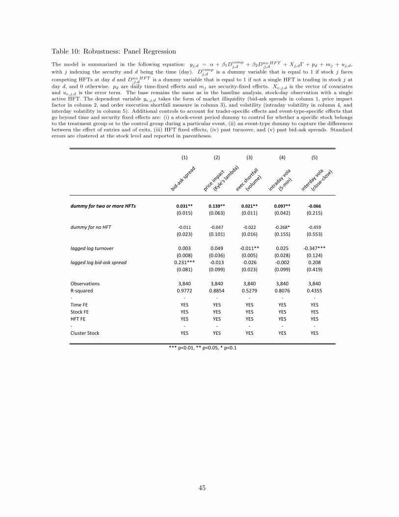
Table 10: Robustness: Panel Regression

The model is summarized in the following equation: yj,d = α + β1Dcomp

j,d+ β2D

no HFT,j,d

+ Xj,dΓ + pd + mj + uj,d,

with j indexing the security and d being the time (day). Dcomp

j,dis a dummy variable that is equal to 1 if stock j faces

competing HFTs at day d and Dno HFT,j,d

is a dummy variable that is equal to 1 if not a single HFT is trading in stock j at

day d, and 0 otherwise. pd are daily time-fixed effects and mj are security-fixed effects. Xe,j,d is the vector of covariatesand ue,j,d is the error term. The base remains the same as in the baseline analysis, stock-day observation with a singleactive HFT. The dependent variable ye,j,d takes the form of market illiquidity (bid-ask spreads in column 1, price impactfactor in column 2, and order execution shortfall measure in column 3), and volatility (intraday volatility in column 4, andinterday volatility in column 5). Additional controls to account for trader-specific effects and event-type-specific effects thatgo beyond time and security fixed effects are: (i) a stock-event period dummy to control for whether a specific stock belongsto the treatment group or to the control group during a particular event, (ii) an event-type dummy to capture the differencesbetween the effect of entries and of exits, (iii) HFT fixed effects, (iv) past turnover, and (v) past bid-ask spreads. Standarderrors are clustered at the stock level and reported in parentheses.

(1) (2) (3) (4) (5)

bid-a

sk spre

ad

price im

pact

(Kyl

e's la

mbda)

exec

short

fall

(volu

me)

intr

aday

vola

(5-m

in)

inte

rday

vola

(clo

se-c

lose

)

dummy for two or more HFTs 0.031** 0.139** 0.021** 0.097** -0.066

(0.015) (0.063) (0.011) (0.042) (0.215)

dummy for no HFT -0.011 -0.047 -0.022 -0.268* -0.459

(0.023) (0.101) (0.016) (0.155) (0.553)

lagged log turnover 0.003 0.049 -0.011** 0.025 -0.347***

(0.008) (0.036) (0.005) (0.028) (0.124)

lagged log bid-ask spread 0.231*** -0.013 -0.026 -0.002 0.208

(0.081) (0.099) (0.023) (0.099) (0.419)

Observations 3,840 3,840 3,840 3,840 3,840

R-squared 0.9772 0.8854 0.5279 0.8076 0.4355

- - - - - -

Time FE YES YES YES YES YES

Stock FE YES YES YES YES YES

HFT FE YES YES YES YES YES

- - - - - -

Cluster Stock YES YES YES YES YES

*** p<0.01, ** p<0.05, * p<0.1

45

Online Appendix

Competition among High-Frequency Traders, and Market Quality

1

A Institutional and Market Background

This section provides institutional details about the Stockholm Stock Exchange for the sample period from June 2009 to

December 2010.

A.A Market Share

Over the sample period, essentially all continuous trading - which is the one relevant for the analysis of high-frequency

trading activity - was taking place on the NASDAQ OMXS. This is one of the key advantages of our dataset for the analysis

of competition as it means we have a comprehensive record of high-frequency trading in a particular security.

Historically, the Stockholm Stock Exchange held all trading in Sweden. By 2009, alternative trading venues BATS Chi-X

Europe, Burgundy and Turquoise held a small share of over-the-counter trading. Today, their shares are significantly higher

and trading is no longer concentrated on one exchange only.

A.B Trading Hours

The limit order book market is open Monday to Friday from 9am to 5:30pm, CET, except on public holidays. Also, trading

closes at 1pm if the following day is a public holiday. Both opening and closing prices are set by call auctions. The priority

rank of an order during the trading day is price, time and visibility.

A.C Account Types

To access the market, financial intermediaries have four different possibilities: (i) Broker accounts are mostly used by

institutional investors or non-automated trader. (ii) An order routing account allows customers of the exchange member

intermediary to route their orders directly to the market. This is mostly used by direct banks such as internet banks. (iii) A

programmed account is used to execute orders through an algorithm such as a big sequential sell or buy order. (iv) Finally,

there is the algorithmic trading account, which is the quickest and the cheapest in terms of transaction costs and thus a

natural choice for HFTs.

A.D Brokers

There are about one hundred financial firms (members) registered at the NASDAQ OMXS.

A.E Hidden Orders

An important detail about the NASDAQ OMXS is that members cannot place small hidden orders. The rule for being able

to hide orders depends on the average daily turnover of a specific stock, but such orders must be at least 50,000EUR. This

figure, however, increases with turnover and reaches, for example, a minimum order size of 250,000EUR for a one million

EUR turnover. As a result, HFTs have no incentive to hide their orders.

B Additional Tables and Figures

Figure A-1 of the Online Appendix provides further details of the tick size changes. Prior to the tick size reform, stocks on

the Stockholm Stock Exchange were exposed to two different tick size tables, Tick Size Table 1 (53% of the stocks) and Tick

Size Table 2 (47% of the stocks). The two different tick size tables were a historical relict and do not reflect any differences

2

in stocks’ liquidity or volatility today. (Historically, stocks traded on the tick size table 1 where younger corporations, while

stocks traded on the tick size table 2 were blue chip stocks.)

The graph on the left-hand-side shows the relevant old and new tick size tables for the Tick Size Table 1 stocks, while the

graph on the right-hand-side shows the table for the Tick Size Table 2 stocks. Nearly all stocks were substantially affected by

the reform, except those stocks that traded on the Tick Size Table 2 and that had stock prices from SEK 100 SEK to SEK

149.99 (level 3 in the right-hand-side graph of Figure A-1). Note that Figure 2 in the main text combines the two graphs,

and depicts the stocks unaffected by the reform using the red dashed line.

3

Figure A-1: Tick Size Tables

This figure depicts tick sizes around the FESE tick size reform on October 26th, 2009 for all relevant price levelsand their corresponding Tick Size Tables on the OMXS30. The graph on the left-hand-side shows the relevant old and newtick size tables for the Tick Size Table 1 stocks, while the graph on the right-hand-side shows the table for the Tick SizeTable 2 stocks. The vertical axis depicts the tick sizes for all relevant price levels.

0.0

5.1

.15

.2.2

5tic

k si

ze (S

EK

)

Oct. 12 Oct. 26 Nov. 6date

level 1 (10 - 49.99 SEK) level 2 (50 - 99.99 SEK)

level 3 (100 - 499.99 SEK)

Tick Size Table 1

0.0

5.1

.15

.2.2

5tic

k si

ze (S

EK

)

Oct. 12 Oct. 26 Nov. 6date

level 1 (40 - 49.99 SEK) level 2 (50 - 99.99 SEK)

level 3 (100 - 149.99 SEK) level 4 (150 - 499.99 SEK)

Tick Size Table 2

Figure A-2: Bid-Ask Spreads

This figure depicts the relative bid-ask spreads around the FESE tick size reform on October 26th, 2009 for allrelevant price levels and their corresponding Tick Size Tables on the OMXS30. The graph on the left-hand-side shows therelative bid-ask spreads for the Tick Size Table 1 stocks, while the graph on the right-hand-side shows the relative bid-askspreads for the Tick Size Table 2 stocks. The vertical axis depicts the relative bid-ask spreads for all relevant price levels.

0.1

.2.3

.4bi

d-as

k sp

read

(%)

Oct. 12 Oct. 26 Nov. 6date

Tick Level 1 (10 - 49.99 SEK) Tick Level 2 (50 - 99.99 SEK)

Tick Level 3 (100 - 499.99 SEK)

Tick Size Table 1

0.1

.2.3

.4bi

d-as

k sp

read

(%)

Oct. 12 Oct. 26 Nov. 6date

Tick Level 1 (40 - 49.99 SEK) Tick Level 2 (50 - 99.99 SEK)

Tick Level 3 (100 - 149.99 SEK) Tick Level 4 (150 - 499.99 SEK)

Tick Size Table 2

4

Table A-1: Summary Statistics of Sample Stocks

This table presents summary statistics for the NASDAQ OMXS30 during the sample period June 2009 throughJanuary 2010. It lists the ISIN code, the company’s name, number of daily trades, daily volume (in 1000 units), dailyturnover (in 1000 SEK) and the relative time-weighted bid-ask spread.

ISIN Code Secuity Name

CH0012221716 ABB Ltd

FI0009000681 Nokia Corporation

GB0009895292 AstraZeneca PLC

SE0000101032 Atlas Copco AB A

SE0000103814 Electrolux, AB B

SE0000106270 Hennes & Mauritz AB, H & M B

SE0000107419 Investor AB B

SE0000108227 SKF, AB B

SE0000108656 Ericsson, Telefonab. L M B

SE0000112724 Svenska Cellulosa AB SCA B

SE0000113250 Skanska AB B

SE0000115446 Volvo, AB B

SE0000122467 Atlas Copco AB B

SE0000148884 Skandinaviska Enskilda Banken A

SE0000163594 Securitas AB B

SE0000171100 SSAB AB A

SE0000193120 Svenska Handelsbanken A

SE0000202624 Getinge AB B

SE0000242455 Swedbank AB A

SE0000255648 ASSA ABLOY AB B

SE0000308280 SCANIA AB B

SE0000310336 Swedish Match AB

SE0000314312 Tele2 AB ser. B

SE0000412371 Modern Times Group MTG AB B

SE0000427361 Nordea Bank AB

SE0000667891 Sandvik AB

SE0000667925 TeliaSonera AB

SE0000695876 Alfa Laval AB

SE0000825820 Lundin Petroleum AB

SE0000869646 Boliden AB

Mean

Trades

Mean SD

2316 1077

1545 570

2455 863

3331 947

3142 1311

4236 1677

1805 516

2798 1016

5986 2019

2266 818

2109 811

4171 943

1250 460

4651 1679

1659 782

2746 917

2255 963

1535 518

5454 2076

2270 897

1351 636

1446 499

2216 854

1485 537

3577 1389

3406 955

2688 1390

2215 674

1790 515

4241 1485

2749 1648

Volume (1000)

Mean SD

2829 1338

1205 502

1321 452

5224 1605

2701 1372

2060 774

1924 702

3082 1432

17108 8753

2154 862

1965 914

6984 2183

1163 510

11070 4734

1940 1063

2820 1049

1786 641

887 473

11386 5355

2070 1009

906 387

1012 386

2001 1111

355 154

9194 3447

5497 1768

9271 5183

2225 962

1436 481

5188 2019

3922 4722

Turnover (1000SEK)

Mean SD

388568 176143

110902 47003

418987 143539

488603 150242

439715 223536

831174 313182

247540 90601

350031 168788

1197412 617496

208511 84315

213179 99676

472870 149712

97269 43480

513746 211720

131865 73863

306488 109205

338677 117238

113873 58061

765288 376062

249035 120835

82726 35999

148239 55642

198433 107238

110940 47783

672128 260518

431676 138283

440023 259887

193898 79892

86773 28329

423193 167698

357223 324766

Bid-Ask Spread

Mean SD

0.173 0.050

0.112 0.013

0.132 0.058

0.140 0.054

0.139 0.051

0.093 0.044

0.177 0.053

0.124 0.036

0.109 0.034

0.118 0.037

0.139 0.045

0.103 0.049

0.186 0.064

0.169 0.094

0.156 0.050

0.198 0.069

0.189 0.101

0.169 0.060

0.226 0.140

0.130 0.043

0.239 0.096

0.143 0.050

0.131 0.016

0.182 0.049

0.145 0.036

0.133 0.054

0.167 0.075

0.114 0.035

0.174 0.038

0.156 0.071

0.153 0.070

5

Table A-2: Correlation Matrix

This table provides correlations between all illiquidity, volatility and high-frequency trading measures we use in the analysis. Illiquidity measures are: bid-askspreads, order execution shortfalls (based on trades and volume), Amihud’s measure of illiquidity, price impact as measured by Kyle’s lambda, and autocorrelation (measureof price efficiency). Volatility measures contain: intraday volatilities (5-minutes and min-max) and interday volatilities (close-close and open-close). High-frequency tradingmeasures are: price pressure measures (based on trades and volume) and three directional trading measures.

bid-a

sk spre

ad

exec

short

fall

(tra

des)

exec

short

fall

(volu

me)

illiq

uidity

(Am

ihud)

price im

pact

(Kyl

e's la

mbda)

price e

ffic

iency

(auto

corr

)

intr

aday

vola

(5-m

in)

intr

aday

vola

(min

-max)

inte

rday

vola

(clo

se-c

lose

)

inte

rday

vola

(open-c

lose

)

price p

ress

ure

(volu

me)

price p

ress

ure

(tra

des)

direct

ional

tradin

g 1

direct

ional

tradin

g 2

bid-ask spread 1

exec shortfall (trades) -0.70 * 1

exec shortfall (volume) -0.43 * 0.46 * 1

illiquidity (Amihud) 0.17 * -0.09 * -0.03 1

price impact (Kyle's ʎ) 0.07 * -0.14 * -0.08 * 0.17 * 1

price efficiency (autocorr) -0.14 * 0.14 * 0.11 * 0.00 0.05 1

intraday vola (5-min) 0.32 * -0.14 * 0.08 * 0.02 0.03 0.05 1

intraday vola (min-max) 0.02 0.00 0.00 -0.02 -0.01 0.01 0.12 * 1

interday vola (close-close) -0.02 -0.02 0.01 -0.01 -0.01 0.02 0.18 * 0.06 * 1

interday vola (open-close) -0.02 0.03 0.05 -0.01 0.11 * 0.03 0.04 0.03 0.00 1

price pressure (volume) -0.30 * 0.35 * 0.20 * -0.06 -0.04 0.04 -0.01 -0.03 -0.05 0.02 1

price pressure (trades) -0.33 * 0.38 * 0.23 * -0.08 * -0.04 0.05 -0.02 -0.03 -0.05 0.05 0.87 * 1

directional trading 1 -0.03 0.13 * 0.03 0.19 * 0.25 * -0.04 0.12 * -0.01 -0.05 0.02 -0.05 0.04 1

directional trading 2 -0.03 0.05 -0.04 0.19 * 0.26 * -0.06 * 0.05 -0.01 -0.06 * 0.02 -0.07 * -0.02 0.82 * 1

directional trading 3 -0.06 * 0.07 * -0.04 0.19 * 0.25 * -0.03 -0.03 0.00 -0.07 * 0.02 -0.05 0.00 0.81 * 0.87 *

* p<0.05

6