First version, November 1, 1999

Current version, November 1, 2000

Competing Against Bundles

Barry NalebuffSchool of Management

Yale UniversityBox 208200

New Haven, CT 06520-8200barry.nalebuff@yale.edu

(203) 432–5968

Abstract: In this paper, we show that a firm that sells a bundle of complementaryproducts will have a substantial advantage over rivals who sell the component productsindividually. Furthermore, this advantage increases with the size of the bundle. Oncethere are four or more items, the bundle seller does better than when it sells eachcomponent individually. This model helps explain one factor in how Microsoft achieveddominance in the Office software suite against pre-existing and well-established rivalsin each component. This paper is a sequel to Bundling as an Entry Barrier [Nalebuff(1999)].

This paper was prepared for ”Incentives, Organization, and Public Economics: Pa-pers in Honour of Sir James Mirrlees,” Oxford University Press. One of the manythings I learned from Professor Mirrlees in the Nuffield College classrooms was thevalue of taking the dual perspective. My heartfelt thanks go Adam Brandenburger,Erik Brynjolfsson, Jeremy Bulow, Avinash Dixit, Jon Levin, Richard Zeckhauser, andseminar participants at Stanford and UCLA, whose perceptive comments led me totackle this problem.

1. Introduction

One of the distinguishing features of our modern economy is the competitive success

achieved by product bundles, Microsoft Office being the case in point. It has achieved

a commanding market share over previously dominant firms selling individual software

applications, such as WordPerfect, Quattro or Lotus, Adobe PageMill, and Harvard

Graphics. While no one single factor explains Microsoft’s success, one part of the

explanation can be found in the writings of Cournot (1838).1 But this is not the

classic Cournot oligopoly model that has become the textbook standard. Instead, it

is Cournot’s dual.

The classic Cournot oligopoly model has a limited number of commodity sellers

each choosing a quantity to put out in the market.2 With linear demand, price is

determined by

p = A− β ∗ (q1 + q2 + . . .+ qn). (1)

As Cournot himself realized, it is entirely possible to flip the ps and qs. Here, the

goods are complements rather than substitutes, and the strategic variable becomes

price, not quantity:

q = A− β ∗ (p1 + p2 + . . .+ pn). (2)

In this interpretation, consumers are interested in buying a collection of n comple-

mentary products, hardware and software, for example. Each of the products is sold

separately at price pi. When determining whether or not to purchase this bundle,

the consumer takes into account the aggregate cost. Thus, a computer user examines

the cost of hardware and software; a student looks at the cost of tuition, room and

board; a skier considers the price of lodging, transportation, lift tickets, equipment,

and lessons.

In Cournot’s own words (Chapter IX “Of the Mutual Relation of Producers”):

We imagine two commodities, (a) and (b), which have no other use beyond

that of being jointly consumed in the production of the composite commodity

1 Other explanations include the delay by Novell and others in updating their products to becompatible with Windows in its migration from DOS.

2 Although the standard textbook model is Cournot quantity competition, there are few real mar-kets — perhaps the Fulton fish market — which satisfy this characterization. It is rare to find a firmthat simply dispenses some quantity of goods on the market and then accepts the market price. In-stead, firms set prices, taking into account the expected prices set by other firms and the anticipateddemand at those prices. Price setting setting can still lead to Cournot-like outcomes as demonstratedby Kreps and Scheinkman (1983). They show that Cournot quantity competition is equivalent toBertrand price competition in a two-stage game where firms first pick capacity levels and then choosequantities in a capacity-constrained second period. This greatly expands the applicability of theCournot model. However, in an economy increasingly dominated by knowledge goods and whereincreasing returns to scale are the order of the day, firms rarely face capacity constraints.

1

(ab). ... Simply for convenience of expression we can take for examples copper,

zinc, and brass under the fictitious hypothesis that copper and zinc have no

other use than that of being jointly used to form brass by their alloy.

In Cournot’s analysis, each component that goes into the bundle is unique — one

type of hardware and one type of software. There is a monopoly in each component.

How, then, will the components will be priced? Cournot shows that if the two monop-

olists get together, they will price the bundle of their goods lower than if they acted

individually.

The two-firm case illustrates the general result. One firm sets the price of good 1

and the other set the price of good 2. With A = 1 and β = 1, the equilibrium has

each firm setting a price of 13 . The bundle price is then 2

3 and total sales are then 13 .

This result should seem familiar. As Sonnenschein (1968) observed, the mathematics

are exactly the same as with the standard Cournot-Nash equilibrium, only here we

have switched prices for quantities and complements for substitutes. Consider what

happens if the two firms get together and coordinate their pricing decision. Now they

would choose p1 + p2 = 0.5, and joint profits would rise from 0.22 to 0.25.

While it is not surprising that coordinated pricing leads to higher profits, what

might be surprising is that coordinated pricing leads to a reduction in prices. Both

consumers and firms are better off.3 The reason is that, in the case of complementors,

when one firm lowers its price, the other firm’s sales increase, an externality that

is not taken into account with uncoordinated pricing. Thus, there is an advantage

to bundling when two firms each have market power, but each is missing one of the

complementary products.4

In this paper, we take the next step in this dual to the Cournot model. We

examine what happens when there is imperfect competition between the component

products that go into the bundle. There are three cases to consider: component

against component, bundle against bundle, and bundle against components.

In the first case, each component is sold separately — hardware against hardware

and software against software. The second scenario considers bundle against bundle

3 The fact that coordination leads to higher profits suggests that a company that sells two comple-mentary products will have a higher incentive to innovate than when the products are sold separately[see Heeb (1998)].

4 It is interesting to note that Posner (1979) looked at the case for bundling pure complements.He concluded that, as consumers care only about the price of the bundle, there would be no point intrying to leverage a monopoly in A to B so as to raise the price of B above its otherwise competitivelevel. Raising the price of A would do just as well. The surprise is that this argument no long holdswhen B is sold by an oligopoly. Because its price lies above the competitive level, the A monopolywants to use its leverage to lower the price of B.

2

— a hardware-software package competes against a rival package.5 The third case

presents bundle against uncoordinated component sellers. Here we have a hardware-

software package competing against independent sellers of hardware and software.

Our interest is in the third case, bundle against components. We use the first two

scenarios to form our basis for comparison. This allows us to better understand what

happens when a player in the market aggregates a collection of complements and sells

them as a bundle, while the competition remains independent or uncoordinated.

Following the intuition of Cournot, it will not be surprising that the bundler does

better than the collection of independent competitors. But the scale of the advantage

is remarkable. Once there are four or more items to the bundle, the bundle aggregator

does better than the sum of its previous parts. And this outcome is stable, as the

disadvantaged independent sellers do not have an incentive to form a rival bundle. This

is because the resulting “ruinous” competition of bundle against bundle would leave

the independent sellers even worse off than they are in their present disadvantaged

position.

Therefore, the results of this paper suggest that a firm that creates or simply

aggregates a bundle of complementary software applications would have a substantial

pricing advantage over its rivals and thereby achieve a leadership position in the

market. This is especially true as the bundle grows in scale. Thus, Microsoft’s taking

the lead in creating a software application bundle — putting together word-processing,

spreadsheet, presentation, HTML editing, and email applications — may help explain

the stunning market success of Microsoft Office suite.

This paper also helps explane how Freeserve gained the lead over AOL as the dom-

inant Internet service provider in the UK. Consumers in this market pay a metered

charge for local telephone service. In this case, the model suggests that Freeserve’s

success was due, in part, to the fact that Freeserve provided a bundle of internet

connectivity and phone service, while AOL customers paid separately for phone con-

nection and internet connection.

2. The Model

Consumers are interested in purchasing a product bundle, which is made up of

several components. We assume that for each component, i, there are two competing

5 The first two scenarios are closely related to the work of Matutes and Regibeau (1989, 1992).Their papers ask the whether or not competing firms would make their products compatible andwhether or not it would be advantageous to sell them in bundles. After we have presented the modeland our results, we return to explain the relationship between our papers.

3

alternatives in the market, Ai and Bi. The Ai and Bi components are imperfect

substitutes. We imagine that the “A” components are all located at 0, while the “B”

components are all located at 1.

We further assume that the consumer gets the value of the products only if all the

components are purchased. Thus, in the case of a two-good bundle, each consumer

will buy one of (A1, A2), (A1, B2), (B1, A2), or (B1, B2). The value of the package is

sufficiently large (relative to the equilibrium prices charged) so that all consumers will

purchase one or the other bundle. Each consumer is interested in exactly one unit of

the bundle.

Consumers assemble the package that best suits their preferences. Each consumer

purchases the bundle with the smallest total cost, where total cost is comprised of

price plus a linear transportation cost. The cost of component i to consumer of type

α is αi + pAi for the Ai product and (1 − αi) + pBi for the Bi product. We assume

that α is uniformly distributed over the unit hypercube.

We further assume that production cost is zero, although with constant marginal

costs, everything perfectly translates into markup over cost.

In a series of models, we will examine the pricing equilibrium that results for

various bundle sizes and market structures. We begin with the simplest case, two

firms, A and B, each selling a one-component product. A one-product bundle is the

limiting case of a bundle.

For firm A, demand and profits are:

DA = 0.5 + 0.5 ∗ (pB − pA). (3)

ΠA = pA ∗DA.

For firm B, the functions are symmetric. This leads to the following first-order con-

ditions

DA − (0.5) ∗ pA = 0; (4)

DB − (0.5) ∗ pB = 0.

In equilibrium, prices equal 1 and the market is evenly split between firms A and

B.

pA = pB ; DA = DB = 1/2; pA = pB = 1. (5)

More generally, this result holds true for any number of components. The only

subtlety is how to interpret the nature of the competition when there are multiple

4

components. For example, assume that there are two A components (A1, A2) and

two B components (B1, B2). In this case, there would be four firms, two A firms

each selling one of the A components and two B firms, each selling one of the B

components.

Each consumer will purchase two components (A1 or B1, A2 or B2). He evaluates

how far he is from each of the items on a component-by-component basis. For example,

a customer located at α = (0.1, 0.5) has a strong preference for A1 and is indifferent

between A2 and B2. Customers are allowed to mix and match in forming their own

bundles. Consequently, consumers optimize their purchase decision component-by-

component. With a uniform distribution of α (on the unit hypercube), this leads us

back to the one-component product case.

PA1 = PA2 = PB1 = PB2 = 1. ΠA1 = ΠA2 = ΠB1 = ΠB2 =12.

This case is the baseline from which we can evaluate the impact of coordinated

pricing decisions. In this baseline case, consumers mix and match their preferred

components and pay a price of n for their n-good customized bundle.

3. Bundle Against Bundle

Next, we consider the case where all the A firms coordinate their pricing and sell

their product as a bundle against the B firms, who have also coordinated their pricing

decisions. We assume that consumers buy only one of the two bundles.6

Let bundle A sell for an amount PA = PA1 + PA2 + . . .+ PAn, and bundle B sell

for PB defined similarly. We assign ∆ to represent the price premium of bundle B

over bundle A, ∆ = PB − PA.

A consumer of type α will prefer to purchase the A bundle over the B bundle if

α · 1 ≤ n+ ∆2

. (6)

Recall that our consumers are uniformly distributed over the unit hypercube. With

n goods in the bundle and a price difference of ∆, the demand for bundle A is thus

D(∆, n) =1n!

n∑k=0

(−1)k(n

k

)max[0, (n+ ∆)/2− k]n. (7)

6 Even if the two technologies are compatible, equilibrium prices are too high to justify buyingboth bundles until n ≥ 4. At n = 4, some consumers would buy both bundles in order to mix andmatch. In the n = 4 equilibrium we calculate below, bundle prices are 1.5; thus, the consumer oftype α = (0, 0, 1, 1) would buy both bundles in order to consume A1, A2, B3, B4. We simplify ouranalysis by assuming that the A and B products are incompatible so that consumers must buy onlyone or the other.

5

For the two-good case, n = 2, and demand simplifies to

D(∆, 2) = (1/2)[(1 + ∆/2)2 − 2 max (0,∆/2)2]. (7′)

As expected at ∆ = 0, demand is 0.5. At ∆ = 2, even the consumer located at (1,1)

is just willing to “travel” the extra distance of 2 to purchase the A bundle at (0,0) in

order to save an extra $2 in price; thus, all of the consumers will go to A, and demand

for bundle A will be 1.

We now calculate the symmetric duopoly equilibrium.7 Firm A maximizes ΠA:

ΠA = PA ∗D(∆, n), ∆ = PB − PA. (8)

The first-order conditions are

D(∆, n) + PAD′(∆, n) = 0. (8′)

At the symmetric equilibrium, ∆ = 0 and D(0, n) = 1/2. Thus, PA = PB =

−1/[2D′(0, n)] where8

D′(0, n) = −(1/2) ∗ [1

(n− 1)!

n∑k=0

(−1)k(n

k

)max[0, n/2− k]n−1] = 0. (9)

For n = 2, this simplifies to

D′(0, 2) = −12

=> PA = 1, ΠA = 1/2. (10)

Profits fall by 50% — we repeat, by 50%. Profits fall by 50% because the aggregate

bundle price has fallen by 50%. The price of the entire bundle is reduced to the

prior price of each of the single components. In hindsight, the intuition is relatively

straightforward. Cutting price brings the same number of incremental customers as

when selling individual components. So the bundle price must equal the individual

price in a symmetric equilibrium.

As the number of elements in the bundle increases, the equilibrium price rises, but

slowly.

7 We would normally call this a Bertrand duopoly. Although Cournot was the first to considera pricing game among complementary products, calling this a Cournot equilibrium would be tooconfusing.

8 When n is even, the calculation of D′(0, n) requires some care since the k = n/2 term in thesummation is not differentiable at ∆ = 0. But because max[0, n/2− k]n−1 = 0 for n ≥ 2 at k = n/2,the left and right hand derivatives with respect to ∆ are equal and so no problem arises.

6

Size of Bundle Bundle Price Market Share Firm Profits

2 1.00 0.50 0.503 1.33 0.50 0.664 1.50 0.50 0.755 1.67 0.50 0.836 1.82 0.50 0.917 1.95 0.50 0.97

Bundle against bundle is ferocious competition. To put this in perspective, in the

seven-good case, if each of the goods were sold separately the price would add up to

7, rather than 1.95, and industry profits would be 3.5 times bigger. From the firms’

perspective, the problem with bundle-versus-bundle competition is that the stakes

are too high. Lowering the price of any one component increases the sale of all n

components. The result is that the component prices fall down to such a low level

that those incremental sales, all combined, are just enough to offset the loss in margin.

We can use the normal approximation to calculate the limiting result as n gets

large. We know that the sum of any number of independent distributions approaches

the normal. In this case, the value of each component has a uniform distribution

over [0,1] with mean 1/2 and variance 1/12. Thus, the density approaches a normal

with mean n/2 and variance n/12. The density at the mean f(µ) = 1/√

2πσ2 =

1/√

2π(n/12) =√

6/πn.

At the symmetric equilibrium, price is simply 1/f(µ), which implies

PA(n) = PB(n) ≈√πn/6. (11)

The equilibrium bundle price rises with the square root of n when competition is over

bundles, while the bundle price rises with n when components are sold individually.

4. Bundle Against Components

We are now ready to consider the case of interest: bundle against components.

The pricing externality suggests that the bundler will have an advantage over the

component sellers. But the results of the previous section suggest that this gain may

be offset by an increase in competition induced by the A firms selling their products

only as bundle. Which effect dominates?

We start with the case where the A and B components are incompatible. This

simplifies the analysis, as consumers must choose between buying the A bundle or

7

buying all the B components and thereby assembling a B-bundle. In the Appendix, we

allow a consumer to buy B components along with the A bundle (since A components

are not sold individually, the reverse case isn’t applicable).

Just as before, a consumer of type α will prefer to purchase the A bundle over the

B bundle if

α · 1 ≤ n+ ∆2

. (12)

With n goods in the bundle and a price difference of ∆, again the demand for

bundle A is

D(∆, n) =1n!

n∑k=0

(−1)k(n

k

)max[0, (n+ ∆)/2− k]n. (13)

The mathematics of bundle against components are very similar to those of bundle

against bundle. The significant difference from the previous section’s analysis is that

there is no one firm B making a coordinated pricing decision. Instead, each of the B

component firms sets its own price. Hence, there is no longer a symmetric equilibrium.

The first-order conditions for firm A and the n firm Bs are:

PAD′ = −D,

PBiD′ = −(1−D), {i = [1, n]}. (14)

This implies:

∆ = [D(∆, n)− n(1−D(∆, n))]/D′(∆, n). (15)

Where D(∆, n) is defined in (13) and

D′(∆, n) = −12

[1

(n− 1)!

n∑k=0

(−1)k(n

k

)max[0, (n+ ∆)/2− k]n−1

](16)

The ∆ that solves (15) is the equilibrium price gap between the A bundle and the

B bundle. Plugging this back into (14) reveals the equilibrium values of PA and PBi .

In general, (15) is best solved via computer. But when n = 2, the solution can be

found directly.9

∆ = [D − 2(1−D)]/D′

= [3D − 2]/D′, (17)

9 Note that in calculating the solution below, we assume that ∆ ≤ 2 and show this assumption isjustified.

8

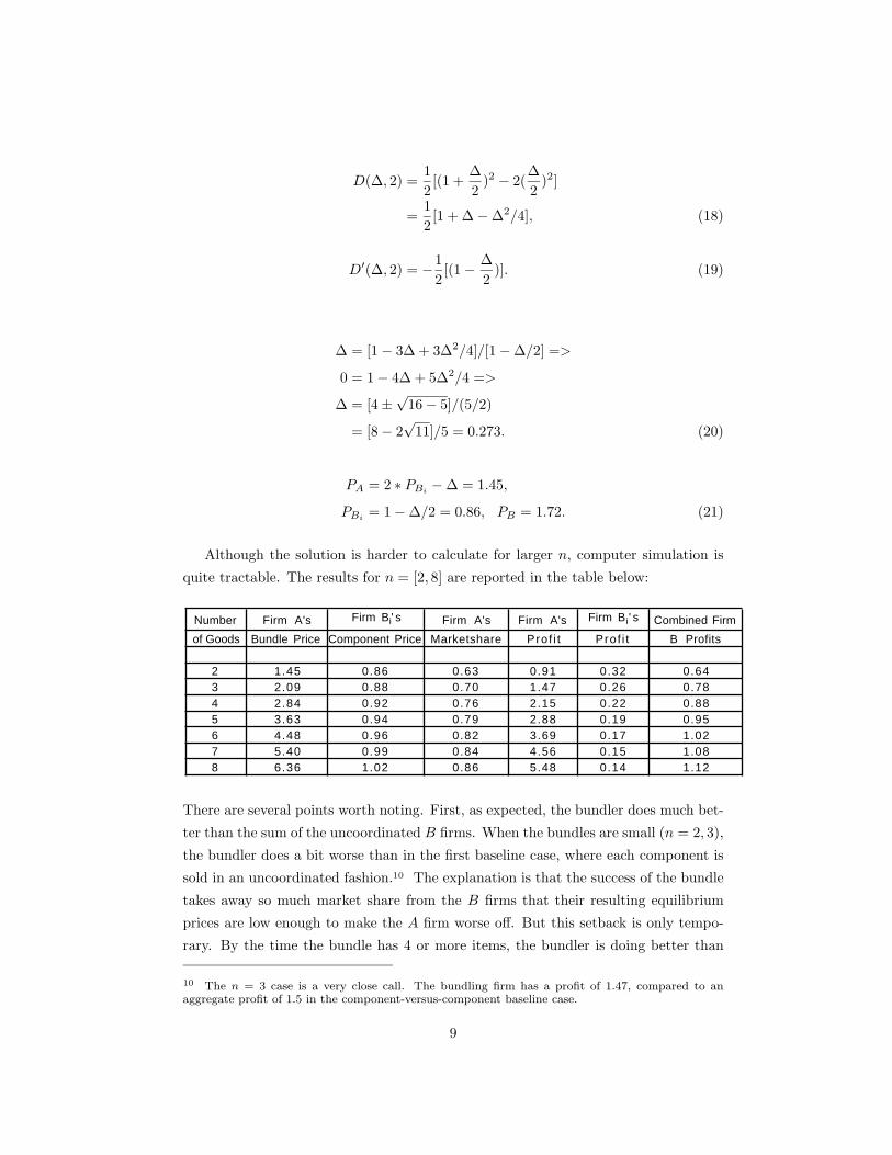
Number Firm A's Firm Bi' s Firm A's Firm A's Firm Bi' s Combined Firm

of Goods Bundle Price Component Price Marketshare Prof i t Prof i t B Profits

2 1.45 0.86 0.63 0.91 0.32 0.643 2.09 0.88 0.70 1.47 0.26 0.784 2.84 0.92 0.76 2.15 0.22 0.885 3.63 0.94 0.79 2.88 0.19 0.956 4.48 0.96 0.82 3.69 0.17 1.027 5.40 0.99 0.84 4.56 0.15 1.088 6.36 1.02 0.86 5.48 0.14 1.12

D(∆, 2) =12[(1 +

∆2

)2 − 2(∆2

)2]

=12[1 + ∆−∆2/4], (18)

D′(∆, 2) = −12[(1− ∆

2)]. (19)

∆ = [1− 3∆ + 3∆2/4]/[1−∆/2] =>

0 = 1− 4∆ + 5∆2/4 =>

∆ = [4±√

16− 5]/(5/2)

= [8− 2√

11]/5 = 0.273. (20)

PA = 2 ∗ PBi −∆ = 1.45,

PBi = 1−∆/2 = 0.86, PB = 1.72. (21)

Although the solution is harder to calculate for larger n, computer simulation is

quite tractable. The results for n = [2, 8] are reported in the table below:

There are several points worth noting. First, as expected, the bundler does much bet-

ter than the sum of the uncoordinated B firms. When the bundles are small (n = 2, 3),

the bundler does a bit worse than in the first baseline case, where each component is

sold in an uncoordinated fashion.10 The explanation is that the success of the bundle

takes away so much market share from the B firms that their resulting equilibrium

prices are low enough to make the A firm worse off. But this setback is only tempo-

rary. By the time the bundle has 4 or more items, the bundler is doing better than

10 The n = 3 case is a very close call. The bundling firm has a profit of 1.47, compared to anaggregate profit of 1.5 in the component-versus-component baseline case.

9

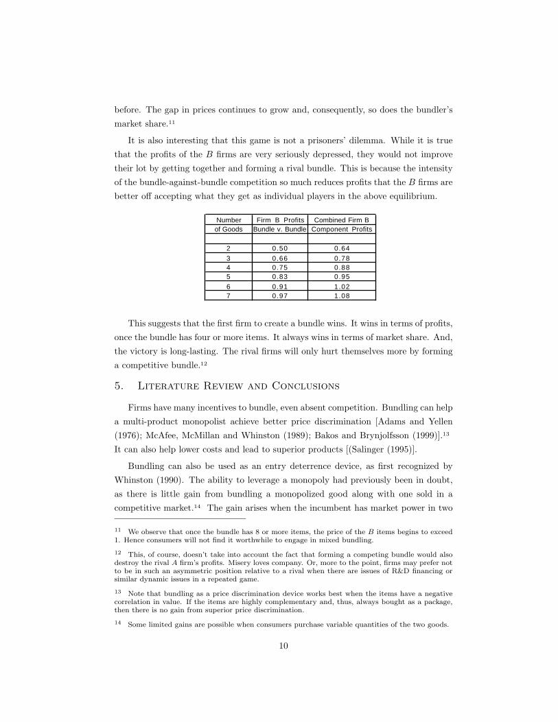
Number Firm B Profits Combined Firm Bof Goods Bundle v. Bundle Component Profits

2 0.50 0.64

3 0.66 0.784 0.75 0.885 0.83 0.95

6 0.91 1.027 0.97 1.08

before. The gap in prices continues to grow and, consequently, so does the bundler’s

market share.11

It is also interesting that this game is not a prisoners’ dilemma. While it is true

that the profits of the B firms are very seriously depressed, they would not improve

their lot by getting together and forming a rival bundle. This is because the intensity

of the bundle-against-bundle competition so much reduces profits that the B firms are

better off accepting what they get as individual players in the above equilibrium.

This suggests that the first firm to create a bundle wins. It wins in terms of profits,

once the bundle has four or more items. It always wins in terms of market share. And,

the victory is long-lasting. The rival firms will only hurt themselves more by forming

a competitive bundle.12

5. Literature Review and Conclusions

Firms have many incentives to bundle, even absent competition. Bundling can help

a multi-product monopolist achieve better price discrimination [Adams and Yellen

(1976); McAfee, McMillan and Whinston (1989); Bakos and Brynjolfsson (1999)].13

It can also help lower costs and lead to superior products [(Salinger (1995)].

Bundling can also be used as an entry deterrence device, as first recognized by

Whinston (1990). The ability to leverage a monopoly had previously been in doubt,

as there is little gain from bundling a monopolized good along with one sold in a

competitive market.14 The gain arises when the incumbent has market power in two

11 We observe that once the bundle has 8 or more items, the price of the B items begins to exceed1. Hence consumers will not find it worthwhile to engage in mixed bundling.

12 This, of course, doesn’t take into account the fact that forming a competing bundle would alsodestroy the rival A firm’s profits. Misery loves company. Or, more to the point, firms may prefer notto be in such an asymmetric position relative to a rival when there are issues of R&D financing orsimilar dynamic issues in a repeated game.

13 Note that bundling as a price discrimination device works best when the items have a negativecorrelation in value. If the items are highly complementary and, thus, always bought as a package,then there is no gain from superior price discrimination.

14 Some limited gains are possible when consumers purchase variable quantities of the two goods.

10

(or more) goods. In Whinston’s model and in related work by Aron and Wildman

(1998), a monopolist’s commitment to bundling makes it a tougher competitor to a

one-good entrant. By committing to a bundle, the firm uses its surplus in good A to

cross-subsidize good B, the one under attack. This denies market share to the entrant,

often enough to deter it from entering. One qualification to these results is that if

entry does occur, bundling ends up hurting the incumbent and, thus, there must be

some way to credibly commit to a bundling strategy.

A companion work to this paper [Nalebuff (1999)] re-examines bundling as an

entry deterrent using a Stackelberg pricing game. Here, too, an incumbent firm with

a monopoly in several components can help protect these multi-monopolies from entry

by bundling them together. This occurs because a one-product entrant faces a very

restricted market compounded by a low incumbent price, all of which makes entry

much less profitable. And now credibility is not an issue, as the incumbent does better

using a bundle against an entrant compared to losing a head-to-head competition on

one of the components.

These models leave open the issue of multi-product entry (or sequential entry by

independent firms). This paper helps us better understand how bundling can change

the nature of competition, post entry. Of course, it is difficult to come up with two or

more products so as to have simultaneous entry. But having done so, there are much

lower profits available to an entrant if the incumbent has a bundle in the market. If

the challenger comes in with a bundle, everyone’s profits are very depressed. If two

firms come in at the same time (or if a latent firm becomes active with the second

firm’s entry), here, too, the entrants’ profits are greatly reduced compared to when

the incumbent sells its product as components or when the incumbent is, in fact, two

separate monopolies, each selling its one component.

The results of this paper are perhaps closest to the work of Matutes and Regibeau

(1989, 1992). They consider a model with two firms, each selling two goods. They

ask whether or not these two firms would choose to make their products compatible

and whether or not the firms would prefer to sell their products as a bundle. In

our initial two baseline cases, the two approaches essentially converge. First, consider

component-versus-component competition. If all the components are compatible, then

there is no externality created by lowering the price of one, and, thus, there is no

gain from getting the two A firms (or the two B firms) to coordinate their pricing.15

15 Matutes and Regibeau do not assume that valuations are all sufficiently high so that everyconsumer makes a purchase. When the market is not all served, there would be a small advantageas lower prices expand the market. Because the whole market may not be served, their paper alsois better designed to examine consumer welfare implications. In our case, component selling is

11

Therefore, our four-firm oligopoly and their two-firm duopoly yield the same outcome.

In the case of bundle-versus-bundle competition, the number of firms falls from four

to two and, thus, is a duopoly model. We, too, observe that bundle-versus-bundle

competition leads to the lowest profits — and the result only gets worse as the bundle

size grows beyond two goods.

Our third scenario, the model of a bundler versus component sellers, is where the

two approaches truly diverge. We are able to focus on the coordination problem of

component sellers against a bundler.16 This is the imperfect competition extension to

Cournot’s multi-product monopoly model. We also see that the results from two-good

bundles may turn around as the bundle grows in scope. The disadvantage of creating a

two-good bundle essentially disappears when there are three goods and even becomes

an advantage once there are four or more items together.

Putting all of these results together leads to a fuller picture of bundling. As

powerful as bundling is to a monopolist, the advantages are even larger in the face

of actual competition or potential competition. Selling products as a bundle can

raise profits absent entry, raise profits even against established but uncoordinated

firms, all the while lowering profits of existing or potential entrants and putting these

rivals in the no-win position of not wanting to form a competing bundle. The only real

disadvantage of bundling is the potential cost of inefficiently including items consumers

don’t desire. This is less important when the items are complementary and when the

marginal cost is essentially zero, as with information goods. Thus, we can expect

bundling to be one of the more powerful and prevalent tools, perhaps we should say

weapons, in our information economy.

unambiguously the best since all consumers, by mixing and matching, will end up with their most-preferred package. The bundle-versus-bundle option restricts choice and, therefore, reduces socialwelfare. The bundle versus components is even worse for social welfare because prices are no longersymmetric. Consequently, consumers who should naturally prefer the B firm products are inducedto travel inefficiently far in order to get the lower price on the A bundle.

16 This coordination problem doesn’t arise in Matutes and Regibeau’s duopoly model as one firmsells both A products and the other sells both B products.

12

6. References

Adams, William J. and Yellen, Janet L. 1976. “Commodity Bundling and the Burden of

Monopoly.” Quarterly Journal of Economics, 90 (Aug.): 475–98.

Aron, Debra and Wildman, Steven. 1998. “Effecting a Price Squeeze Through Bundled

Pricing,” working paper Northwestern University.

Bakos, Yannis and Brynjolfsson, Eric. 1999. “Bundling Information Goods: Pricing,

Profits, and Efficiency,” Management Science, forthcoming

Cournot, Augustin. 1838. Recherches sur les principes mathematiques de la theorie des

richesses, Paris: Hachette. English translation: (N. Bacon, trans.), Research into

the Mathematical Principles of the Theory of Wealth (James and Gordon, Mountain

Center: CA 1995)

Heeb, Randal. 1998. “Innovation and Vertical Integration in Complementary Software

Markets,” University of Chicago Ph.D. thesis.

Kreps, David and Scheinkman, Jose. 1983. “Quantity Precommitment and Bertrand

Competition Yield Cournot Outcomes,” Bell Journal of Economics, 14(2): 326–37.

Matutes, Carmen and Regibeau, Pierre. 1989. “Standardization across Markets and

Entry,” Journal of Industrial Economics, 37: 359–372.

Matutes, Carmen and Regibeau, Pierre. 1992. “Compatibility and Bundling of Comple-

mentary Goods in a Duopoly,” Journal of Industrial Economics, 40(1): 37–54.

McAfee. R. Preston, McMillan, John, and Whinston, Michael D. 1989. “Multiproduct

Monopoly, Commodity Bundling, and Correlation of Values,” Quarterly Journal of

Economics, 104 (May): 371–84.

Nalebuff, Barry. 1999. “Bundling as an Entry Barrier,” working paper available online at

Social Science Research Network http://papers.ssrn.com/paper.taf?abstract id=185193

Salinger, Michael A. 1995. “A Graphical Analysis of Bundling,” Journal of Business, 68

(Jan.): 85–98.

Sonnenschein, Hugo. 1968. “The Dual of Duopoly Is Complementary Monopoly: or, Two

of Cournot’s Theories Are One,” The Journal of Political Economy , 76(2): 316–318.

Whinston, M. D. 1990. “Tying Foreclosure, and Exclusion,” American Economic Review ,

80 (Sept.): 837–59.

Posner, Richard. 1979. “The Chicago School of Antitrust Analysis,”University of Penn-

sylvania Law Review , 127: 925.

13

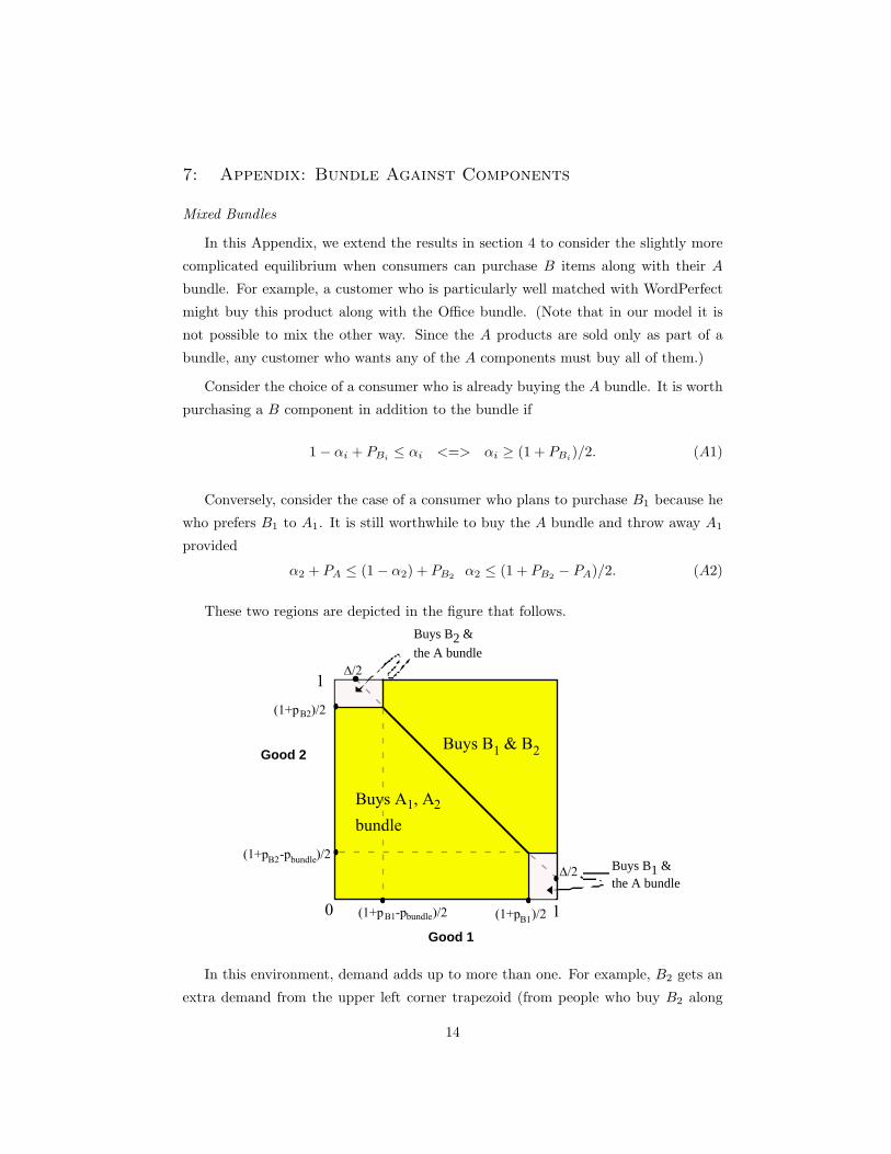
1

1

0 (1+pB1-pbundle)/2

Buys B1 & the A bundle

(1+pB1)/2

(1+pB2)/2

(1+pB2-pbundle)/2

∆/2

∆/2

Buys B2 &

the A bundle

Buys B1 & B2

Buys A1, A2

bundle

Good 2

Good 1

7: Appendix: Bundle Against Components

Mixed Bundles

In this Appendix, we extend the results in section 4 to consider the slightly more

complicated equilibrium when consumers can purchase B items along with their A

bundle. For example, a customer who is particularly well matched with WordPerfect

might buy this product along with the Office bundle. (Note that in our model it is

not possible to mix the other way. Since the A products are sold only as part of a

bundle, any customer who wants any of the A components must buy all of them.)

Consider the choice of a consumer who is already buying the A bundle. It is worth

purchasing a B component in addition to the bundle if

1− αi + PBi ≤ αi <=> αi ≥ (1 + PBi)/2. (A1)

Conversely, consider the case of a consumer who plans to purchase B1 because he

who prefers B1 to A1. It is still worthwhile to buy the A bundle and throw away A1

provided

α2 + PA ≤ (1− α2) + PB2 α2 ≤ (1 + PB2 − PA)/2. (A2)

These two regions are depicted in the figure that follows.

In this environment, demand adds up to more than one. For example, B2 gets an

extra demand from the upper left corner trapezoid (from people who buy B2 along

14

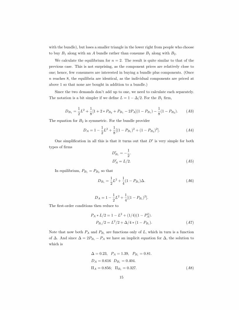
with the bundle), but loses a smaller triangle in the lower right from people who choose

to buy B1 along with an A bundle rather than consume B1 along with B2.

We calculate the equilibrium for n = 2. The result is quite similar to that of the

previous case. This is not surprising, as the component prices are relatively close to

one; hence, few consumers are interested in buying a bundle plus components. (Once

n reaches 8, the equilibria are identical, as the individual components are priced at

above 1 so that none are bought in addition to a bundle.)

Since the two demands don’t add up to one, we need to calculate each separately.

The notation is a bit simpler if we define L = 1−∆/2. For the B1 firm,

DB1 =12L2 +

18[1 + 2 ∗ PB2 + PB1 − 2PA](1− PB1)−

18(1− PB2). (A3)

The equation for B2 is symmetric. For the bundle provider

DA = 1− 12L2 +

18[(1− PB1)

2 + (1− PB2)2]. (A4)

One simplification in all this is that it turns out that D′ is very simple for both

types of firms

D′Bi = −12.

D′A = L/2. (A5)

In equilibrium, PB1 = PB2 so that

DBi =12L2 +

14(1− PBi)∆. (A6)

DA = 1− 12L2 +

14[(1− PBi)2].

The first-order conditions then reduce to

PA ∗ L/2 = 1− L2 + (1/4)(1− P 2A).

PBi/2 = L2/2 + ∆/4 ∗ (1− PBi). (A7)

Note that now both PA and PBi are functions only of L, which in turn is a function

of ∆. And since ∆ = 2PBi − PA we have an implicit equation for ∆, the solution to

which is

∆ = 0.23, PA = 1.39, PBi = 0.81.

DA = 0.616 DBi = 0.404.

ΠA = 0.856; ΠBi = 0.327. (A8)

15

Once again the bundler dominates the individual component sellers. Prices for

both firms are a little lower (1.39 versus 1.45 for firm A and 0.81 versus 0.86 for the

B firms), as each firm can now expand the market with lower prices. The lower prices

are almost exactly offset by the increase in total demand so that profits are almost

unchanged. Thus, although the mathematics are more complicated, the intuition and

the results are very similar to those in Section 4.

16