HAL Id: halshs-01180812https://halshs.archives-ouvertes.fr/halshs-01180812

Preprint submitted on 28 Jul 2015

HAL is a multi-disciplinary open accessarchive for the deposit and dissemination of sci-entific research documents, whether they are pub-lished or not. The documents may come fromteaching and research institutions in France orabroad, or from public or private research centers.

L’archive ouverte pluridisciplinaire HAL, estdestinée au dépôt et à la diffusion de documentsscientifiques de niveau recherche, publiés ou non,émanant des établissements d’enseignement et derecherche français ou étrangers, des laboratoirespublics ou privés.

Competence versus Honesty: What Do Voters CareAbout?

Fabio Galeotti, Daniel John Zizzo

To cite this version:Fabio Galeotti, Daniel John Zizzo. Competence versus Honesty: What Do Voters Care About?. 2015.�halshs-01180812�

WP 1520 – July 2015

Competence versus Honesty:

What Do Voters Care About?

Fabio Galeotti, Daniel John Zizzo

Abstract:

We set up an experiment to measure voter preferences trade-offs between competence and honesty. We measure the competence and honesty of candidates by asking them to work on a real effort task and decide whether to report truthfully or not the value of their work. In the first stage, the earnings are the result of the competence and honesty of one randomly selected participant. In the second stage, subjects can select who will determine their

earnings based on the fi rst stage’s competence and honesty of the alternative candidates.

We find that most voters tend to have a bias towards caring about honesty even when this results in lower payoffs.

Keywords: Voting preferences, competence, honesty, election

JEL codes: C72, C91, D72

1

Competence versus Honesty: What Do Voters Care About?

Fabio Galeotti Université de Lyon, Lyon, F-69007, France ; CNRS, GATE Lyon Saint-Etienne, Ecully, F-

69130, France

Daniel John Zizzo* Newcastle University

Version: July 2015

Abstract

We set up an experiment to measure voter preferences trade-offs between competence and honesty. We measure the competence and honesty of candidates by asking them to work on a real effort task and decide whether to report truthfully or not the value of their work. In the first stage, the earnings are the result of the competence and honesty of one randomly selected participant. In the second stage, subjects can select who will determine their earnings based on the first stage’s competence and honesty of the alternative candidates. We find that most voters tend to have a bias towards caring about honesty even when this results in lower payoffs.

Keywords: voting preferences, competence, honesty, election.

JEL classification numbers: C72, C91, D72.

* Corresponding author. E-mail: daniel.zizzo@ncl.ac.uk. Phone: +44 (0)191 208 5844; address: Newcastle University Business School and BENC, 5 Barrack Road, Newcastle upon Tyne, NE1 4SE, United Kingdom. We received helpful comments from Friedel Bolle, Yves Breitmoser, Enrique Fatas, Sebastian Fehrler, Steffen Huck, Alex Karakostas, Joshua Miller, Antonio Nicolò, Abhijit Ramalingam, Elke Renner, Pieter Serneels, Theodore Turocy, Georg Weizsäcker and seminar participants in Berlin (WZB), Besançon (5th Annual Meeting of ASFEE), Birmingham, East Anglia (CBESS), ESC Dijon, Lyon (GATE-LSE, HEIDI-CORTEX workshop), Maastricht (M-BEES 2014), Montpellier, Newcastle, Erlangen-Nuremberg and Shanghai (5th Annual SEBA-GATE Workshop). We gratefully acknowledge financial support by CBESS and University of East Anglia. We also thank Marie Aguirre, Quentin Thevebet, and Ailko van der Veen for experimental assistance in the laboratory. The usual disclaimer applies.

2

1. Introduction

We present an experiment on the preferences of voters over candidates in public

elections. We are interested in two main characteristics that define the quality of a candidate:

competence and honesty.1 Competence refers to the ability of a potential public official to

properly perform his/her job, identifying and employing the appropriate policies that enable

her to get the job done. Honesty refers to the general attitude of the potential public official to

fulfill the trust that the voters have placed on him or her; it usually implies a general aversion

towards dishonest practices such as bribery, kickbacks, and public embezzlement which

would benefit the public official to the detriment of the public; it can be understood within a

fiduciary model of duty in politics according to which the public official behaves honestly in

order to fulfil the trust of those who voted for him or her (Besley, 2005).2

Why may people have a preference over one of the two characteristics that define the

quality of a public official? From a traditional economic point of view, a rational and purely

self-interested voter should always select the candidate that ensures the highest expected

return for the elector irrespectively of everything else. The underlying idea – well captured by

Bill Clinton’s 1992 presidential campaign strategist James Carville in his slogan “[it’s] the

economy, stupid” – is that people care only about the economy and want candidates who are

able to improve it, and therefore their own financial position, irrespectively of everything else.

The results of this study will tell us whether this is true or not based on the preferences of the

voters over the characteristics of the candidates. In addition, our experiment may help us

understand why democracies may at times suffer from endemic dishonesty and corruption at

the public level. If voters in fact display a rational and profit-maximizing voting behavior or a

preference for competence over honesty, the existence of corruption and dishonesty in

modern democracies might be explained by people's voting preferences.

Voters may however be reluctant to support a dishonest candidate if, for instance,

they display what has been referred as “betrayal aversion”, that is a general dislike to “being

1 There are indubitably other aspects that may affect the quality of a public official. However, as Besley (2005, p. 47) pointed out, “their merits are more difficult to assess”. 2 In a previous study by Caselli and Morelli (2004), the authors used the same two characteristics to define the quality of a public official. Besley (2005) also used the term honesty to identify, along with competence, the principal dimensions of the quality of politician, and he interpreted it as “a duty of rulers to uphold the public trust” (Besley, 2005: pp. 48-49). From a more general perspective, competence and honesty can also be associated to the two universal dimensions of human social cognition: competence or efficiency, on the one side, and perceived warmth or trustworthiness, on the other side (in social psychology, see, e.g., Fiske et al., 2007; Fiske et al., 2002; in economics, see Butler and Miller, 2014).

3

betrayed beyond the mere payoff consequences” (Bohnet et al., 2008, p. 295), or if they care

more about the process by which the payoffs are generated rather than the final payoffs (see,

e.g., Rabin, 1993). Similarly, voters may be sensitive to a social norm that prescribes to

punish a candidate who proves to be dishonest. As a result, voters may vote for a candidate

who is more reliable but overall less worthwhile than the contender in terms of expected

payoffs.

The opposite, also plausible, possibility is that voters may support the more competent

candidate, quite independently of the honesty of the alternative candidates and the expected

returns associated to each of them. This may be the case if, for instance, voters think that the

misuse of public power for personal benefit at the public level is a fact of life and, hence,

justified (Peters and Welch, 1980) or if there is so much distrust in the public system that

voters believe that the election of a honest public official would have no impact whatsoever

on the system or only a marginal one.3

There are other possible explanations of why voters choose a certain candidate which

abstract from the pure preferences of the voters over honesty and competence. Most notably,

voters can be affected by the quality and level of information on the candidates available to

them at the moment of the vote (Peters and Welch, 1980).4 In this study, we do not

investigate the impact of these other factors that may affect the decision making of the voters

in elections, but we focus solely on the voters’ preferences over honesty and competence, in a

context where the candidates differ only over these two characteristics and where the voters

are fully informed about them.

There are many examples of real-world situations which could be used to support

either the primacy of honesty or that of competence for voting behavior. For instance, the

success of the anti-establishment movement of the comedian Beppe Grillo at the general and

local elections in Italy over the 2012 and 2013 might be explained by a greater weight

assigned by a significant proportion of voters to honesty rather than competence. Many voters

might have voted for Grillo’s party because of its choice to propose ordinary voters as

candidates, with no experience on politics and public offices, but, as Grillo emphasized

3 According to the 2014 corruption perception index published by the Transparency Organization (http://www.transparency.org/cpi2014), many countries do indeed present very high perceived levels of corruption in the public sector that could justify a total disinterest of the voters in the honesty of the candidates. 4 Other important aspects that may influence the electoral choices of the voters are, for example, the electors’ partisanship to a certain ideology or party or the sensitivity of certain electors to some attractive characteristics of a candidate such as beauty or charisma.

4

during his political campaign, much more honest than conventional politicians (Bartlett,

2013). A dislike of voters for dishonest candidates may also explain why, in certain cases,

candidates affected by corruption scandals fail to be elected or experience a significant drop

in voters’ support. For instance, in the elections of the US House of Representatives Peters

and Welch (1980) and Welch and Hibbing (1997) found that incumbent candidates touched

by corruption allegations lost more often their seats and received about 10% less than

incumbent candidates with no corruption accusations.

A significant number of other cases seem however to support the opposite conjecture

that voters are motivated by their final expected payoffs or care more about the competence

of candidates rather than the honesty. For instance, many of the parliamentarians who were

involved in the 2009 UK parliamentary expenses scandal5 held their seats in the 2010 general

elections and experienced only a marginal drop in voters’ support (about 1.5% on average;

Eggers and Fischer, 2011). In Brazil, the former Brazilian President Luis Inacio Lula da Silva

won the 2006 general elections regardless of the corruption scandals that plagued his

previous administration and after a mandate characterized by steady economic growth and

decrease in poverty for Brazil (Winters and Weitz-Shapiro, 2013).

Although these examples may provide important insights on how voters vote in public

elections, they cannot be used to infer the preferences of voters over honesty and competence

as many other factors may have played a role in voting decisions. Research is needed to

uncover these preferences and isolate them from other influences. Furthermore, in modern

democratic elections, the vote is secret and anonymous. As a result, real-world data on voters’

preferences is typically collected only in aggregate form after an election or via public

opinion polls or surveys. However, aggregate data are usually difficult to interpret due to the

lack of control over many unobservable variables, in primis the individual characteristics of

the voters. In addition, the answers of voters to surveys and public opinion polls can be

highly affected by social pressure, especially because voters are asked about sensitive topics

such as political preferences, and, therefore, not fully reliable (DeMaio, 1984).

By means of a lab experiment, we are able to bypass these limitations. We can collect

data on individual voting behavior which is usually difficult to analyze with standard

empirical approaches. In our experiment, we ask voters to select a public official, based on

5 In 2009, several members of the UK parliaments misused their permitted allowances and made inappropriate expenses claims for personal benefits.

5

the competence and honesty of which their final payoffs depend. We measure the competence

of the candidates in a real effort task and their honesty by asking them to truthfully or

untruthfully report the value produced in the real effort task. We then provide this

information to the voters and ask them to select the public official. By looking at cases where

there is a competence-honesty trade-off, we can then measure the extent to which competence

and honesty matter in electoral decisions, or whether in the end only the expected financial

bottom line for voters matters. We find that most voters in general tend to have a bias towards

caring about honesty irrespectively of whether this maximizes their earnings or not.

The remaining of the paper is organized as follows. Section 2 reviews the literature

related to this study. Section 3 presents the experimental design. Section 4 describes the

hypotheses to be tested and the theoretical background. Section 5 presents the results. Section

6 briefly presents the design and results of a second experiment. Sections 7 and 8 discuss the

findings and conclude, respectively.

2. Related literature

To the best of our knowledge, there is no study that investigates the extent to which

competence and honesty matter in electoral decisions. That said, one strand of related

literature is about electoral delegation. In our experiment, a subject is chosen by some voters

to be the public official and act for them. Several studies investigate the behavioral

implications of delegating a decision about outcomes to another person (e.g. Otto and Bolle,

2013; Hamman et al., 2011; Bolle and Vogel, 2010; Samuelson and Messick, 1986;

Samuelson et al., 1984; Messick et al., 1983). These studies focus primarily on the delegate’s

behavior and its implications in term of welfare rather than the preferences of the people over

the characteristics of the potential delegates. Similarly, voting preferences on the

characteristics of the potential leaders is not a topic covered in the economic research on

leadership, whereas it is the focus of our paper.6

6 A public official can be in fact seen in many respects as a leader. The literature on leadership mostly focuses on the impact of leading-by-example (e.g. Gäcther et al., 2012; Güth et al., 2007; Potters et al., 2007; Moxnes and van der Hejden, 2003). Some papers compare the implications of having randomly selected leaders with elected leaders (e.g. Levy et al., 2011; Brandts et al., 2012; Kocher et al., 2013), leaders appointed based on their past contribution (e.g. Gäcther and Renner, 2005), leaders appointed based on participant’s performance in a pre-task (e.g. Kumru and Vesterlund, 2010), and self-selected leaders (e.g. Rivas and Sutter, 2011; Arbak and Villeval, 2011). In our experiment, the “leader” is endogenously selected, as in some of this research. However, in contrast to this literature, our study is not about leadership-by-example, and we are not interested on the leader and followers’ behavior but on subjects’ preferences over the characteristics of the potential leaders.

6

Another stream of literature related to our study is about honesty in decision making.

In our experiment, voters are asked to elect a public official who could breach the fiduciary

relationship that he or she holds with his or her constituency, and behave dishonestly by

underreporting the value of a common fund for personal benefits. Economists have

empirically investigated dishonesty mostly using experimental data. Some have studied lying

and dishonesty in cheap talk games where some players can send true or false message

regarding some kind of private information (e.g. future moves) to other players (e.g. Sutter,

2009; Gneezy, 2005; Croson, 2005). In these studies, deception is totally disclosed to the

experimenter. Other scholars – not only in economics – have studied unobserved lying

behavior and lying aversion by tracing its distribution from subjects’ reported results of a dice

roll, coin flip or matrix task (e.g. Fischbacher and Heusi, 2013; Hao and Houser, 2013;

Abeler et al., 2014; Houser et al., 2012; Bucciol and Piovesan, 2011; Mazar and Ariely,

2006).

Our study is also related to some research on corruption. Barr at al. (2009) and Azfar

and Nelson (2007) used a Public Servant’s Game to study corruption in service delivery. In

this game, one subject is assigned the role of service provider (or executive), a second subject

the role of monitor (or attorney general), and the remaining subjects (6 subjects) are

community members. The decision of the service provider, that is how many tiles (from a

random distribution) to allocate to the community, is similar to the one of the public official

in our experiment. A few economists and political scientists have also examined the extent to

which voters may support corrupted incumbents in public elections (e.g. Peters and Welch,

1980; Welch and Hibbing, 1997; Ferraz and Finan, 2008; Winters and Weitz-Shapiro, 2013;

Bågenholm, 2013). These studies are to some extent linked to ours since corruption may be a

sign of dishonesty, particularly if the interests of the voters are aligned with those of the

public. These works primarily used aggregate-level empirical approaches and focus solely on

the impact of corruption on incumbents’ re-election without investigating the trade-off

between honesty and competence.7

There is political science research studying the importance of the quality of the

candidates, defined as a combination of integrity and competence, in electoral choices

(Mondak and Huckfeldt, 2006; Mondak, 1995; Kulisheck and Mondak, 1996; McCurley and

7 An exception is the political study of Winters and Weitz-Shapiro (2013), who employed a non-incentivized survey experiment to investigate the attitude of respondents towards hypothetical incumbent politicians (vignettes) described in the form of qualitative sentences.

7

Mondak, 1995). Mondak (1995) investigated the permanence of incumbents in the US House

of Representatives in relation to the quality of the incumbents, measured as an index of

competence and integrity constructed with content analysis. He found that high-quality US

House members remained in office longer than low-quality members. McCurley and Mondak

(1995) combined the aggregate-level data on the quality of US House of Representatives’

incumbents with individual-level post-election survey data to explore whether the skill and

integrity of the candidates affect the voters’ evaluation of the candidates and their voting

choice. They found that the quality scores do affect the evaluation of the candidates. Similar

findings are provided by Kulisheck and Mondak (1996) who investigated whether the

information concerning the quality of hypothetical candidates influences the voting choice of

subjects in a survey experiment. Mondak and Huckfeldt (2006) collected data from a series of

survey experiments and a national survey to study the accessibility of the competence and

integrity of hypothetical candidates in the evaluation of the contenders, and how people

respond to these characteristics relative to partisanship and ideology. They found that

competence and integrity are slightly more accessible than partisanship and ideology, and are

perceived favorably by subjects. Altogether these studies provide evidence that the quality of

candidates matter in national elections. However, they are inconclusive on which dimension

of the quality matters the most. In addition, they present several features in relation to which

our laboratory experiment approach based on an incentivized environment is able to provide

a significant contribution.8

3. Experimental design

To investigate the preferences of voters over the competence and honesty of

candidates in public elections, we conduct a main experiment in France (Experiment 1) and a

complementary one in UK and France (Experiment 2).9 In the paper, we mainly focus on

Experiment 1, and only briefly discuss the other experiment. More details on Experiment 2

can be found in Galeotti and Zizzo (2014).

8 First, when aggregate-level empirical approaches are used (e.g. Mondak, 1995; McCurley and Mondak, 1995), it is usually difficult to isolate and control for the effects of important unobservable variables, such as, for instance, the information available upon the candidates. In addition, one can question the subjectivity and precision of the measure used to identify the quality of a candidate, and the reliability of post-election surveys to measure the voters’ support for a candidate (see, e.g., DeMaio, 1984; Lodge et al., 1990). Finally, when survey experiments are used (Kulisheck and Mondak, 1996; Mondak and Huckfeldt, 2006), the situations described to the subjects are hypothetical, there are no economic incentives associated with the choices, the focus is more on attitude and perception rather than behavior, and the quality of the candidates is identified only with qualitative statements and phrases. While these comments are not to deny the value of these studies, they suggest that an experimental approach of the kind we use would be especially useful to complement them. 9 Experiment 2 was a preliminary experiment which was ran before Experiment 1.

8

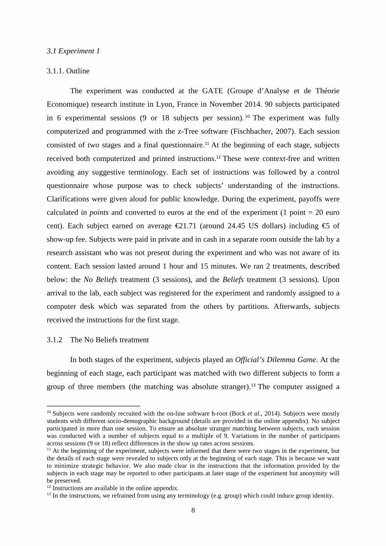
3.1 Experiment 1

3.1.1. Outline

The experiment was conducted at the GATE (Groupe d’Analyse et de Théorie

Economique) research institute in Lyon, France in November 2014. 90 subjects participated

in 6 experimental sessions (9 or 18 subjects per session).10 The experiment was fully

computerized and programmed with the z-Tree software (Fischbacher, 2007). Each session

consisted of two stages and a final questionnaire.11 At the beginning of each stage, subjects

received both computerized and printed instructions.12 These were context-free and written

avoiding any suggestive terminology. Each set of instructions was followed by a control

questionnaire whose purpose was to check subjects’ understanding of the instructions.

Clarifications were given aloud for public knowledge. During the experiment, payoffs were

calculated in points and converted to euros at the end of the experiment (1 point = 20 euro

cent). Each subject earned on average €21.71 (around 24.45 US dollars) including €5 of

show-up fee. Subjects were paid in private and in cash in a separate room outside the lab by a

research assistant who was not present during the experiment and who was not aware of its

content. Each session lasted around 1 hour and 15 minutes. We ran 2 treatments, described

below: the No Beliefs treatment (3 sessions), and the Beliefs treatment (3 sessions). Upon

arrival to the lab, each subject was registered for the experiment and randomly assigned to a

computer desk which was separated from the others by partitions. Afterwards, subjects

received the instructions for the first stage.

3.1.2 The No Beliefs treatment

In both stages of the experiment, subjects played an Official’s Dilemma Game. At the

beginning of each stage, each participant was matched with two different subjects to form a

group of three members (the matching was absolute stranger).13 The computer assigned a

10 Subjects were randomly recruited with the on-line software h-root (Bock et al., 2014). Subjects were mostly students with different socio-demographic background (details are provided in the online appendix). No subject participated in more than one session. To ensure an absolute stranger matching between subjects, each session was conducted with a number of subjects equal to a multiple of 9. Variations in the number of participants across sessions (9 or 18) reflect differences in the show up rates across sessions. 11 At the beginning of the experiment, subjects were informed that there were two stages in the experiment, but the details of each stage were revealed to subjects only at the beginning of each stage. This is because we want to minimize strategic behavior. We also made clear in the instructions that the information provided by the subjects in each stage may be reported to other participants at later stage of the experiment but anonymity will be preserved. 12 Instructions are available in the online appendix. 13 In the instructions, we refrained from using any terminology (e.g. group) which could induce group identity.

9

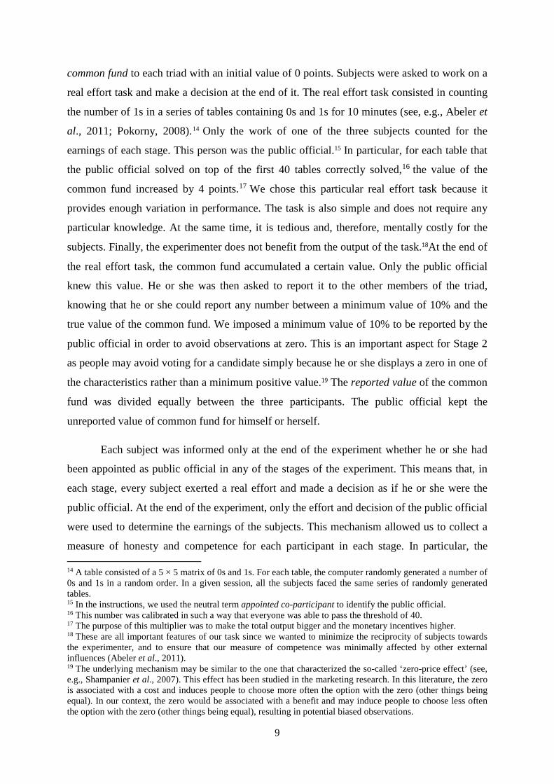
common fund to each triad with an initial value of 0 points. Subjects were asked to work on a

real effort task and make a decision at the end of it. The real effort task consisted in counting

the number of 1s in a series of tables containing 0s and 1s for 10 minutes (see, e.g., Abeler et

al., 2011; Pokorny, 2008).14 Only the work of one of the three subjects counted for the

earnings of each stage. This person was the public official.15 In particular, for each table that

the public official solved on top of the first 40 tables correctly solved,16 the value of the

common fund increased by 4 points.17 We chose this particular real effort task because it

provides enough variation in performance. The task is also simple and does not require any

particular knowledge. At the same time, it is tedious and, therefore, mentally costly for the

subjects. Finally, the experimenter does not benefit from the output of the task.18At the end of

the real effort task, the common fund accumulated a certain value. Only the public official

knew this value. He or she was then asked to report it to the other members of the triad,

knowing that he or she could report any number between a minimum value of 10% and the

true value of the common fund. We imposed a minimum value of 10% to be reported by the

public official in order to avoid observations at zero. This is an important aspect for Stage 2

as people may avoid voting for a candidate simply because he or she displays a zero in one of

the characteristics rather than a minimum positive value.19 The reported value of the common

fund was divided equally between the three participants. The public official kept the

unreported value of common fund for himself or herself.

Each subject was informed only at the end of the experiment whether he or she had

been appointed as public official in any of the stages of the experiment. This means that, in

each stage, every subject exerted a real effort and made a decision as if he or she were the

public official. At the end of the experiment, only the effort and decision of the public official

were used to determine the earnings of the subjects. This mechanism allowed us to collect a

measure of honesty and competence for each participant in each stage. In particular, the 14 A table consisted of a 5 × 5 matrix of 0s and 1s. For each table, the computer randomly generated a number of 0s and 1s in a random order. In a given session, all the subjects faced the same series of randomly generated tables. 15 In the instructions, we used the neutral term appointed co-participant to identify the public official. 16 This number was calibrated in such a way that everyone was able to pass the threshold of 40. 17 The purpose of this multiplier was to make the total output bigger and the monetary incentives higher. 18 These are all important features of our task since we wanted to minimize the reciprocity of subjects towards the experimenter, and to ensure that our measure of competence was minimally affected by other external influences (Abeler et al., 2011). 19 The underlying mechanism may be similar to the one that characterized the so-called ‘zero-price effect’ (see, e.g., Shampanier et al., 2007). This effect has been studied in the marketing research. In this literature, the zero is associated with a cost and induces people to choose more often the option with the zero (other things being equal). In our context, the zero would be associated with a benefit and may induce people to choose less often the option with the zero (other things being equal), resulting in potential biased observations.

10

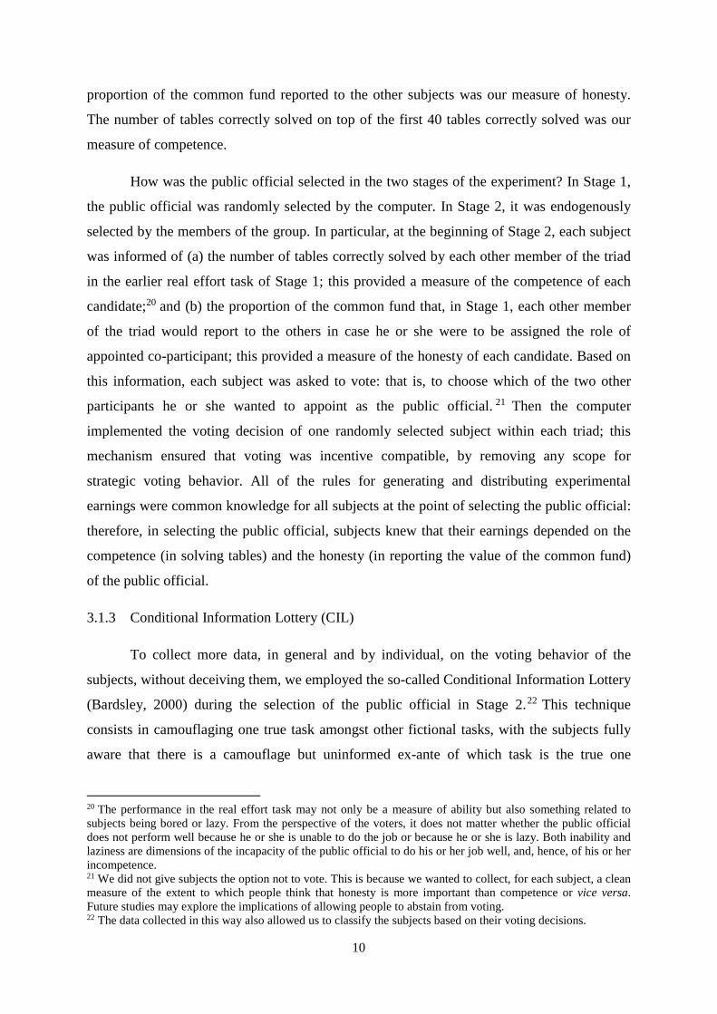
proportion of the common fund reported to the other subjects was our measure of honesty.

The number of tables correctly solved on top of the first 40 tables correctly solved was our

measure of competence.

How was the public official selected in the two stages of the experiment? In Stage 1,

the public official was randomly selected by the computer. In Stage 2, it was endogenously

selected by the members of the group. In particular, at the beginning of Stage 2, each subject

was informed of (a) the number of tables correctly solved by each other member of the triad

in the earlier real effort task of Stage 1; this provided a measure of the competence of each

candidate;20 and (b) the proportion of the common fund that, in Stage 1, each other member

of the triad would report to the others in case he or she were to be assigned the role of

appointed co-participant; this provided a measure of the honesty of each candidate. Based on

this information, each subject was asked to vote: that is, to choose which of the two other

participants he or she wanted to appoint as the public official. 21 Then the computer

implemented the voting decision of one randomly selected subject within each triad; this

mechanism ensured that voting was incentive compatible, by removing any scope for

strategic voting behavior. All of the rules for generating and distributing experimental

earnings were common knowledge for all subjects at the point of selecting the public official:

therefore, in selecting the public official, subjects knew that their earnings depended on the

competence (in solving tables) and the honesty (in reporting the value of the common fund)

of the public official.

3.1.3 Conditional Information Lottery (CIL)

To collect more data, in general and by individual, on the voting behavior of the

subjects, without deceiving them, we employed the so-called Conditional Information Lottery

(Bardsley, 2000) during the selection of the public official in Stage 2.22 This technique

consists in camouflaging one true task amongst other fictional tasks, with the subjects fully

aware that there is a camouflage but uninformed ex-ante of which task is the true one

20 The performance in the real effort task may not only be a measure of ability but also something related to subjects being bored or lazy. From the perspective of the voters, it does not matter whether the public official does not perform well because he or she is unable to do the job or because he or she is lazy. Both inability and laziness are dimensions of the incapacity of the public official to do his or her job well, and, hence, of his or her incompetence. 21 We did not give subjects the option not to vote. This is because we wanted to collect, for each subject, a clean measure of the extent to which people think that honesty is more important than competence or vice versa. Future studies may explore the implications of allowing people to abstain from voting. 22 The data collected in this way also allowed us to classify the subjects based on their voting decisions.

11

(Bardsley, 2000). More specifically, in the selection of the public official, each subject was

presented with ten randomly ordered situations: one real and nine fictional. In the real

situation, each subject was informed about the actual competence and honesty of the other

participants within his or her group. In the fictional situations, each subject was instead

presented with fictitious information about the competence and honesty of the other two

participants. In particular, to make the camouflage credible and realistic, the information used

in the fictional situations came from subjects, chosen at random by the computer, who

participated in Experiment 2 and performed the same task (i.e. Official’s Dilemma Game) of

Experiment 1.23 More specifically, to generate the fictional situations, the computer randomly

combined subjects from past sessions using a stratification procedure which followed

approximately the distribution of the cases observed in the Official’s Dilemma Game of

Experiment 2. In two fictional situations, one candidate strictly or weakly dominated the

other candidate in both characteristics (competence and honesty). All the other seven fictional

situations corresponded to cases where the characteristics of the two candidates were

orthogonal and differed in the extent to which the two candidates were different in terms of

expected payoffs generated for the voter. In particular, in three situations, the difference in

expected payoffs between the two candidates laid in the interval [0, 5] experimental points; in

two other situations, the difference laid in the interval (5, 10] experimental points; in another

situation the difference lay in the interval (10, 20] experimental points; and in another one in

the interval (20, 50] experimental points. This stratified randomization allowed us to provide

to the subjects enough decoys to prevent them from spotting the true situation, and, at the

same time, to collect more information on the electoral choices of subjects for different level

of expected payoffs of the candidates. The order of the ten situations was randomized. For

each situation, each subject was asked to choose which of the two participants he or she

wanted to appoint as the public official, knowing that only the decision of one participant

selected at random in the real situation was implemented.

As Bardsley (2000) pointed out, the CIL procedure might induce “cold” decisions

because of the hypothetical nature of the task. This might actually be desirable in our

experiment as voters do usually make their electoral choices in a “cold” state, since they are

typically asked to vote in polling places, anytime over a span of one or two days and after the

political campaign of the candidates. The CIL procedure may also dilute the incentives of the

23 To generate the fictional situations, we only used subjects who had been appointed as public officials. This is because, in Experiment 2, subjects were informed in advance whether or not they had been appointed as public officials.

12

experiment, and increase the misunderstanding of the experimental procedures. To minimize

these drawbacks, we limited the fictional situations to only ten and made sure that subjects

fully understood the instructions.24 It was also important that subjects did not spot the true

situation. As we have already mentioned earlier, we adopted a procedure of stratified

randomization to select the fictional situations from real situations occurred in past sessions,

making very difficult, if not impossible, for the subjects to identify the true situation. Finally,

in Experiment 2, we ran some sessions without the CIL procedure (i.e. the Baseline treatment)

as a control to check whether any biases were produced from using the CIL procedure. We

find no bias.

3.1.4 The Beliefs treatment

The Beliefs treatment differs from the No Beliefs treatment only in the voting phase

of Stage 2. In particular, for each voting situation, and before choosing one of the two

candidates, subjects were also asked to indicate how many tables they think each candidate

will correctly solve, and what proportion of the common fund they think each candidate will

report. At the end of the experiment, the computer randomly drew, for each participant, one

guess in the real situation. Subjects earned 2 extra euros if their guess was correct. If the

guess was incorrect by � tables (in the case the randomly drawn guess was about the tables

correctly solved) or percentage points (in the case the randomly drawn guess was about the

proportion of the common fund reported), subjects earned max�0, 2 − 0.1�� extra euros. All

the other aspects of the experiment were identical to the No Beliefs treatment.

3.1.5 Final questionnaire

In both the Beliefs and No Beliefs treatments, after Stage 2, subjects had to complete

a 4-parts questionnaire, reproduced in the online appendix.25

3.1.6 Payments

24 As we have already mentioned early, subjects filled in a control questionnaire, followed by clarifications, to check their understanding of the instructions, with key questions regarding, for instance, the meaning of the fictional situations. 25 In part 1, we measured the risk attitude of subjects. We employed the Eckel et al. (2012)’s task in the domain of gains. In this task, subjects had to choose one gamble out of six possible gambles. Each gamble was represented with a circle and involved two payoffs with 50% probability of occurrence each. Moving from gamble 1 to gamble 6, both expected return and risk increased. This part was incentivized. Part 2 was the Stöber (2001)’s 17-item Social Desirability Scale (SDS17 score) which measures how much a person desires to be perceived in a positive light. Part 3 was the Christie and Geis (1970)’s 20-item Machiavellianism scale (MACH score) which measures a person’s tendency to be amoral and opportunist. In the last part of the questionnaire, we collected some demographics and elicited subjects’ belief about the objective of the experiment.

13

At the end of the experiment, the computer randomly drew one of the two stages.

Subjects were paid the earnings of that stage plus the show-up fee of 5 euros and any

additional earnings that they obtained by answering the final questionnaire. In the Beliefs

treatment, they were also paid the earnings of one randomly drawn guess.

4. Theoretical background and hypotheses

In this section, we set the theoretical background and present the hypotheses to be

tested. Let us call �,� the expected earnings of the generic voter n if the candidate j is

appointed. This can be defined as:

�,� = �������

where A is the constant multiplier of voter n’s profit function (equal to 4/3 in our

experiment, where 3 is the group size, and 4 is the value of one table correctly solved by the

candidate on top of the first 40 correct tables and reported to the voter); ��� captures the

honesty of the candidate and is measured as the proportion of the common fund reported by

the candidate to the voters; ��� captures the competence of the candidate and is measured as

the number of tables correctly solved on top of the first 40 tables correctly solved in the real

effort task. The profit function is a Cobb-Douglas with profit elasticities of competence and

honesty equal to 1. Each elasticity measures the responsiveness of the profit to a change in

competence or honesty, ceteris paribus. In particular, a 1% increase in competence would

lead to a 1% increase in profit. Similarly, a 1% increase in honesty would lead to a 1%

increase in profit.

The voter n must choose among two candidates (J =2). The voter obtains a certain

utility if a certain candidate is elected. In particular, the utility that voter n gets if candidate j

is appointed is ��,� , j = 1, 2. Each candidate possesses two attributes (competence and

honesty) which are known by the voter. If the voter is rational and profit maximizing, she

should choose the candidate that gives the highest utility, and her utility should be an

increasing function of the expected earnings. For simplicity, let the utility be a standard

Cobb-Douglas function26 which can be defined as follows:

26 The Cobb-Douglas function has been widely used in economics to identify the production function of a firm or the utility function of an economic agent (see, e.g., Mas-Colell et al., 1995). In our context, it is particularly useful as it allows us to estimate the weights that a voter places on the honesty and competence of the candidates in a directly comparable way. In particular, the weights are expressed in terms of elasticities, that is how much

14

��,� = ���������

�����,�

where �� and �� are the weights (elasticities) of the honesty and the competence

respectively of the candidate j in the utility function of voter n. ���������

�� is the known

component of the utility function, whereas ���,� is the stochastic component (unknown

component).27

If the two attributes have the same weight in the utility (�� = �� = �), the voter cares

only about his or her profit. We can rewrite the utility as a function of the profit:

��,� = �,�����,�

Hypothesis 1. If voters are rational and profit maximizing, �� = �� = �, with � > 0.

If � is equal to 0, the utility does not depend on the profit. If � is less than 0, it

negatively depends on the profit. If �� > �� (�� > ��), it means that the voter weight more

the honesty (competence) of the candidate over the competence (honesty), and over what

would be predicted by profit maximization.

Hypothesis 2. If honesty matters more than competence, �� will be greater than ��.

Hypothesis 3. If competence matters more than honesty, �� will be greater than ��.

To test the Hypotheses 1, 2 and 3, we can take the natural logarithm of the utility to

obtain a linear function in parameters:

ln#��,�$ = %�,� = ln��� + ����� + ����� + '�,�

Knowing that the probability that voter n chooses candidate i over j is:

(�,) = (*+,#%�,) > %�,�$ = (*+,#%�,) − %�,� > 0$

We can derive the logit choice probability assuming that the error term ('�,�) is iid

with a Type-I extreme value distribution. The equation for the logit choice probability is:

the utility varies (in percentage) if honesty or competence increases by 1%. In addition, it is logically consistent with the essential elements of our experiment. In particular, it is directly linked to the profit function used in our experiment. More precisely, it can be reduced to a function of the profit if the weights of honesty and competence are identical. 27 For simplicity, we assume that the stochastic component is non-additive.

15

(�,) = (*+,#%�,) > %�,�$ =exp��� ln#���$ + �� ln#���$�

∑ exp��� ln#���$ + ��ln�������0� �

The estimation of �� and �� is relatively straightforward through maximum

likelihood estimation as we observe the choices of the voters and we have measures of the

honesty and competence of the candidates.

5. Experimental results

In this section, we main focus on the results of Experiment 1. We only briefly

consider some of the findings of Experiment 2 at the end of the section, and report the rest in

the online appendix.

5.1 Experiment 1’s results

5.1.1 Descriptives

Table 1 shows the average measures of competence and honesty from the two stages

of the experiment. In the table, competence is the number of tables correctly solved on top of

the first 40 tables correctly solved in the real effort task; honesty is the proportion of the

common fund that a subject would report if he or she were to be the public official. Both

competence and honesty in Stage 1 were positively correlated with competence and honesty

in Stage 2 (Spearman’s ρ = 0.86 and 0.74, and p < 0.001 for both). This indicates that both

measures were valid proxies of subjects’ behavior in Stage 2. While competence significantly

increased from Stage 1 to 2 (Wilcoxon signed-rank test, p < 0.001), honesty weakly

significantly decreased (p = 0.054). Both trends are probably explained by learning.

[Table 1 about here]

To analyze the electoral choices of subjects, we first consider the number of times

subjects voted for a candidate for each possible electoral situations that occurred in the

experiment (Table 2).28 If we look at the interesting situations where there was a trade-off

between honesty and competence, subjects seemed to vote more often for the honest

candidate as opposed to the more competent one in the No Belief treatment and if we

consider the two treatments pooled together. We can test more formally whether the

proportion of situations where subjects chose the more honest candidate significantly differs

28 Due to a technical problem during the voting stage of one session in the Belief treatment, the information about honesty and competence of some candidates were displayed as 0s in the computer screen of certain voters. This problem affected 12 voting choices which we dropped from the analysis.

16

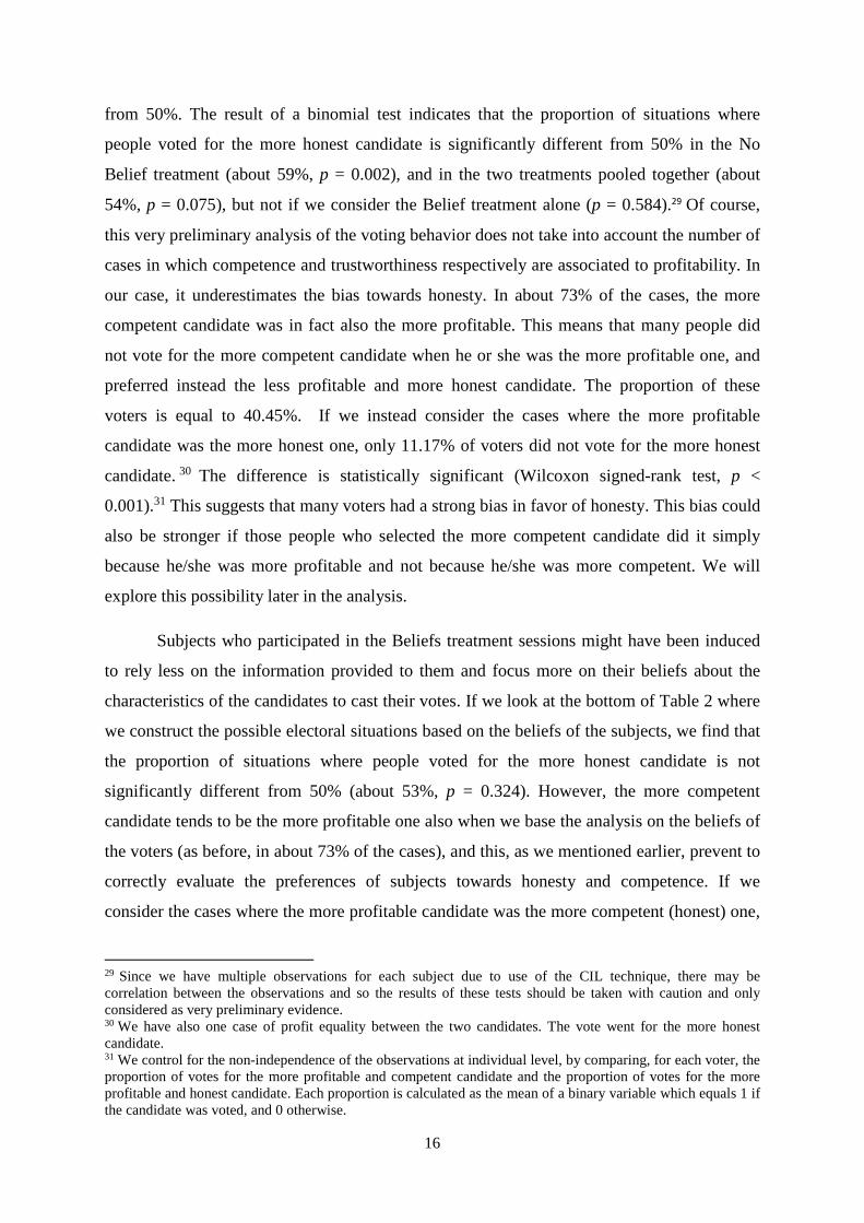
from 50%. The result of a binomial test indicates that the proportion of situations where

people voted for the more honest candidate is significantly different from 50% in the No

Belief treatment (about 59%, p = 0.002), and in the two treatments pooled together (about

54%, p = 0.075), but not if we consider the Belief treatment alone (p = 0.584).29 Of course,

this very preliminary analysis of the voting behavior does not take into account the number of

cases in which competence and trustworthiness respectively are associated to profitability. In

our case, it underestimates the bias towards honesty. In about 73% of the cases, the more

competent candidate was in fact also the more profitable. This means that many people did

not vote for the more competent candidate when he or she was the more profitable one, and

preferred instead the less profitable and more honest candidate. The proportion of these

voters is equal to 40.45%. If we instead consider the cases where the more profitable

candidate was the more honest one, only 11.17% of voters did not vote for the more honest

candidate.30 The difference is statistically significant (Wilcoxon signed-rank test, p <

0.001).31 This suggests that many voters had a strong bias in favor of honesty. This bias could

also be stronger if those people who selected the more competent candidate did it simply

because he/she was more profitable and not because he/she was more competent. We will

explore this possibility later in the analysis.

Subjects who participated in the Beliefs treatment sessions might have been induced

to rely less on the information provided to them and focus more on their beliefs about the

characteristics of the candidates to cast their votes. If we look at the bottom of Table 2 where

we construct the possible electoral situations based on the beliefs of the subjects, we find that

the proportion of situations where people voted for the more honest candidate is not

significantly different from 50% (about 53%, p = 0.324). However, the more competent

candidate tends to be the more profitable one also when we base the analysis on the beliefs of

the voters (as before, in about 73% of the cases), and this, as we mentioned earlier, prevent to

correctly evaluate the preferences of subjects towards honesty and competence. If we

consider the cases where the more profitable candidate was the more competent (honest) one,

29 Since we have multiple observations for each subject due to use of the CIL technique, there may be correlation between the observations and so the results of these tests should be taken with caution and only considered as very preliminary evidence. 30 We have also one case of profit equality between the two candidates. The vote went for the more honest candidate. 31 We control for the non-independence of the observations at individual level, by comparing, for each voter, the proportion of votes for the more profitable and competent candidate and the proportion of votes for the more profitable and honest candidate. Each proportion is calculated as the mean of a binary variable which equals 1 if the candidate was voted, and 0 otherwise.

17

39.57% (11.59%) were willing to sacrifice monetary payoffs to vote for the more honest

(competent) candidate.32 The difference is statistically significant (Wilcoxon signed-rank test,

p < 0.001). This suggests that people had a strong bias toward honesty also when we consider

their beliefs about the competence and honesty of the candidates.

[Table 2 about here]

If we look at the other situations where there is no trade-off between honesty and

competence, in a very small proportion of cases (4.52%),33 subjects displayed what we refer

as an inconsistent voting behavior, that is they voted for the candidate who was strictly

dominated in both characteristics (honesty and competence) by the other candidate. This

proportion is very small in the No Belief treatment (1.72% of cases with inconsistent voting

behavior), and larger in the Belief treatment, both if we consider the actual levels of

competence and trustworthiness (7.62% of cases with inconsistent voting behavior) or the

beliefs (9.36%).34 The behavior of these subjects (from now on, we will label them as

inconsistent subjects) is difficult to characterize and interpret. It is likely that they made

random choices during the experiment or did not take the experiment seriously. Hence, we

will control for their behavior in the remaining of the analysis.

We can also look at how the probability that a candidate i is elected evolves as a

function of the difference in competence and honesty between candidate i and her rival,

candidate j (Figure 1). To make competence and honesty graphically comparable, we

standardized them, that is we subtract the mean from each value and divide the result by the

standard deviation. The graph suggests first that subjects seemed to behave quite rationally as

the probability of being elected was close to 1 when the candidate was superior in both

characteristics compared to the contender (upper corner of the first graph), and was close to 0

when the candidate was inferior in both characteristics (bottom corner of the first graph).

32 We have also 7 cases of profit equality between the two candidates. The vote went for the more honest candidate in 5 cases (71.43%). 33 More precisely, 8 subjects (2 in the No Belief treatment, 6 in Belief treatment) out of 90 displayed this behavior (8.89% of subjects). If we consider the beliefs of subjects, 11 subjects out of 45 (24.44%) displayed inconsistent voting behavior. However, only 4 of them (8.89%) were inconsistent both based on their beliefs and the information provided to them about the competence and honesty of the candidates. The proportion of inconsistent subjects is significantly smaller in the No Belief treatment compared to the Belief treatment only if the inconsistent voting behavior in the Belief treatment is based on the beliefs of the subjects (Fisher’s exact test, p = 0.014). 34 A possible explanation of why there was more inconsistent voting behavior in the Belief treatment compared to the No Belief treatment is that task was more cognitively demanding in the Belief treatment (subjects expressed their beliefs and selected a candidate in ten consecutive voting situations), and, therefore, it was more likely to make a mistake.

18

Second, the subjects seemed to prefer more an honest candidate to a competent one since the

probability of being elected increases more steeply when the difference in honesty between

two candidates increases than when the difference in competence increases. We will

investigate this in more detail in the regression analysis.

[Figure 1 about here]

We now consider the expected payoffs that each candidate provided to the voters. We

begin by assuming that subjects had adaptive expectations, that is they took the measures of

honesty and competence from the earlier stages to estimate what expected payoffs would be

had by each candidate if elected public official. We shall relax this assumption later. First, we

look at the probability of electing the more honest candidate as a function of the difference in

expected payoffs ∆π between the more and less honest candidate (Figure 2), restricting the

analysis to the observations where there was a trade-off between honesty and competence.

The probability is obtained by computing the weighted running means of a dichotomous

variable taking value 1 when the honest candidate is elected and 0 otherwise. For ∆π < 0 (i.e.

the more honest candidate is also the less profitable), profit-maximizing subjects should vote

for the less honest candidate as he or she is associated with higher expected payoffs. Hence,

the area below the smoothed means measures the extent to which subjects voted for the more

honest candidate when this was not the more profitable candidate. For ∆π > 0 (i.e., the more

honest candidate is also the more profitable), profit-maximizing subjects should vote for the

more honest candidate as he or she is associated with higher expected payoffs. Hence, the

area above the smoothed means measures the extent to which subjects voted for the more

competent candidate when this was not the more profitable candidate. Note that the

theoretical predicted probability under rational self-interest would follow a step function

where the voter never chooses the more honest candidate in the region where ∆π < 0, and

always chooses him or her when ∆π > 0.

[Figure 2 about here]

As Figure 2 shows, choices follow fairly a pattern based on the rational self-interested

prediction, in some preliminary support of Hypothesis 1. However, the area below the

weighted running means for ∆π < 0 is bigger than the area above the weighted running means

for ∆π > 0. This preliminary evidence strongly supports Hypothesis 2: subjects seemed more

likely to vote for the less profitable candidate when this was the more honest one. This

19

evidence appears to be stronger in the No Belief treatment, and in the Belief treatment when

we construct the voting situations based on the beliefs of subjects.

To look at this further, we consider how often subjects voted for the more honest

candidate when the latter was the less profitable one, and how often subjects voted for the

more competent candidate when the latter was the less profitable one. Figure 3 reports the

proportion of cases where the voters selected the less profitable candidate for each interval of

absolute deviation in expected payoffs between the two candidates.35 This proportion

identifies the rate of counterintuitive voting behavior and measures the proportion of cases

where subjects are willing to sacrifice their expected monetary payoffs in order to select the

more honest or competent candidate. Both in aggregate and for most of the intervals of

difference in expected payoffs, the proportion of cases where subjects voted for the

unprofitable and more honest candidate was signficaintly larger than the proportion of cases

where subjects voted for the unprofitable and more competenent candidate.36

[Figure 3 about here]

This is preliminary evidence of the fact that voters weighed honesty more than

competence, particularly when the candidates contributed a similar amount to the expected

payoffs of the voters. In terms of the theoretical hypotheses presented earlier, this suggests

that ��is greater than ��, especially when the difference in expected payoffs between the two

candidates is small enough.

5.1.2 Regression analysis

We now make our analysis more rigorous using regression analysis. We identify the

candidate chosen by each voter with a dummy variable ‘Vote’ (= 1 if the candidate is chosen,

0 otherwise). For each situation faced by a generic voter i, we have two observations and for

only one of the two the variable ‘Vote’ is equal to 1. Based on the theoretical background

presented in a previous section, we estimate the probability that a subject votes for a certain

35 These were the same intervals that were used in the design phase of the experiment to generate the fictitious situations. 36 Since the observations are not independent within each subject, a χ2 test would not be valid. To solve this problem, we compute, for each voter and each interval of absolute deviation in expected payoffs between the candidates, the average vote (calculated as the mean of a binary variable which is equal to 1 if the candidate was voted, and 0 otherwise) for the less profitable and more competent candidate, and for the less profitable and more honest candidate respectively. We then compare, for each voter, these two average votes using a Wilcoxon signed-rank test (the p-values are reported in Figure 3). Note that, for certain intervals of absolute deviation, we do not have enough observations. As a result, the statistical power may be very low or the test may not be feasible. The results do not change if we exclude the inconsistent subjects.

20

candidate based on the characteristics of the alternative candidates. In particular, we estimate

an alternative-specific conditional choice model. Since we have multiple observations per

individual, we employ robust standard errors clustered at individual level. The dependent

variable is the dummy ‘Vote’. In Regression 1, the independent variables include the logs of

measured honesty and competence of the candidate, log(honesty) and log(competence). In

Regression 2, we also add interaction terms of these variables with a dummy variable | | > 5,

which takes value 1 when the absolute deviation in expected payoffs between the two

candidates is larger than 5 experimental points. In Regression 3, we also control for the

demographic, psychological and behavioral characteristics of the voters and treatment effects

by interacting them with log(honesty) and log(competence).37 In particular, we control for the

nationality of the subjects (not from France), their gender, their age, whether they study

economics or not, and whether they are undergraduate students or not. In addition, we control

for the risk attitude of the subjects, and their scores in the SDS17 and MACH questionnaires.

We also control for the sessions where we elicited subjects’ beliefs. Additionally, we control

for the behavior of the voters in the first stage of the experiment (own competence and

honesty) by interacting the log of competence and honesty of each voter with the log of the

honesty and competence respectively of the candidates. Finally, we control for the behavior

of the inconsistent subjects by including an interaction of whether a subject was categorized

as inconsistent with log(honesty) and log(competence) respectively. Regressions 4-6 are like

Regressions 1-3 except that we focus only on the Belief sessions, and we measure honesty

and competence with the beliefs of the subjects. Table 3 displays the results of the regressions.

[Table 3 about here]

In Regressions 1 and 4, both the coefficients of the log of honesty (��) and the log of

competence (�� ) are positive and significant. The coefficient of log(honesty) is also

significantly larger than the coefficient of log(competence) (χ2 test, p < 0.001 in both

Regression 1 and 4). We can present the first and second result.

Result 1. Subjects tended to weigh honesty more than competence, as predicted by

Hypothesis 2.

37 Note that since our model is alternative-specific, the characteristics of the voters do not vary over the choices of the voters, and, therefore, they would be dropped out from the model. The only way to get around this problem and account for the individual characteristics of the voter is to add interaction terms between the alternative-specific variables and the voter-specific variables as we do in our regressions.

21

Result 2. The bias towards caring about honesty remains if we assume that subjects

decisions were driven by their beliefs about the honesty and competence of candidates.

Did the bias occur only when the difference in expected payoffs between the

candidates was small enough? Once we control for small and large differences in expected

payoffs between the two candidates (Regressions 2 and 5), the coefficient for log(honesty)

remain significantly larger than the coefficient for log(competence) both for small and large

differences (χ2 test, p = 0.031 for Regression 2, and 0.002 for Regression 5). In other words,

the bias towards caring about honesty seems to caracterize both situations where the

difference in expected payoffs between the candidates is small and large.

Result 3. Subjects tended to weigh honesty more than competence even when the

difference in expected profits between the two candidates was large.

Results 1-3 also hold in Regressions 3 and 6 where we control for the demographic,

psychological and behavioral characteristics of the subjects, and treatment effects from

eliciting the beliefs of the subjects. In particular, the coefficient for log(honesty) is about

twice as large as the coefficient for log(competence) and the difference is statistically

significant (χ2 test, p < 0.001 for Regression 3, and 0.016 for Regression 6).38

So far we have assumed that subjects displayed adaptive expectations, that is they

formed their expectations about how the potential public official will behave in the future

based on the information provided to them regarding the past competence and honesty of the

candidates. It is possible that subjects displayed rational expectations. This means that the

subjects’ expectations about the future honesty and competence of the public official matched

exactly the true expected values of future honesty and competence of the public official. In

the online appendix, we replicate the analysis conducted so far by assuming that subjects

display rational expectations. The results are qualitatively similar to those presented in the

paper, if anything with stronger evidence of an honesty bias. It might also be possible that our

38 Among the controls, in Regression 3, the only coefficients statistically significant are the interaction terms between Inconsistency and log of honesty and competence respectively (negative coefficients, p-values = 0.071 and 0.031), background in economics and log of honesty (negative coefficient, p-value = 0.084), and voter’s honesty and log of honesty and competence respectively (negative coefficients, p-values = 0.081 and 0.049). In Regression 6, the only coefficients statistically significant are the interaction terms between background in economics and log of competence (positive coefficient, p-value = 0.086), and MACH score and log of competence (positive coefficient, p-values = 0.088). To sum up these additional findings, inconsistent subjects, as well as more honest voters, tended to rely less on measured competence and honesty. Subjects with a background in economics put a slightly smaller weight on honesty and a slightly larger weight on their beliefs about competence compared to other subjects. Subjects who scored high in the Machiavellianism scale, tended to weigh more believed competence.

22

results are driven by extreme cases, namely situations where the difference in expected

profits between the two candidates is very large. Hence, we replicate the analysis by dropping

those cases. The results are reported in the online appendix and replicate those presented in

the paper.

5.1.3 Types classification

We now classify subjects based on their pattern of voting behavior. We can do this

since we collected multiple observations of voting behavior for each subject. We identify 7

categories of subjects, and Table 4 summarizes the results of this classification.

[Table 4 about here]

‘Profit-maximizing’ voters. These subjects always selected the more profitable

candidate irrespectively of his or her competence and honesty. In terms of our theoretical

specification, the utility of the ‘profit-maximizing’ voters is characterized by �� = �� > 0. In

a first classification, we only consider those subjects who were profit-maximizing based on

adaptive expectations. In a second classification, we also consider those subjects who were

profit-maximizing based on rational expectations.39 Subjects that do not fall in the ‘Profit-

maximizing’ subjects category are classified as follow.

‘Unconditional competence’ voters. These subjects always selected the more

competent candidate irrespectively of the expected profits. The utility function of these

subjects is characterized by �� > 0 and �� = 0.

‘Unconditional honesty’ voters. These subjects always selected the more honest

candidate irrespectively of the expected profits. Their utility function is represented by �� =

0 and �� > 0.

‘Conditional competence’ voters. These subjects selected more often the competent

candidate than the honest candidate.40 The behavior of these subjects is captured by an utility

function characterized by �� > �� > 0.

39 33.3% of the subjects who are classified as profit-maximizing based on rational expectations, also fit in the category of the subjects who are profit-maximizing based on adaptive expectations. 40 To identify these subjects, we computed, for each subject, the average vote for the honest candidates when these were the least profitable, and compared it with the average vote for the competent candidates when these were the least profitable. If the difference was positive (i.e. the subject more often voted for the less profitable and honest candidate than the less profitable and competent candidate), the subject was categorized as ‘Conditional honesty’ subject. If the difference was negative (i.e. the subject more often voted for the less

23

‘Conditional honesty’ voters. These subjects selected more often the honest candidate

than the competent candidate. The behavior of these subjects is captured by an utility

function characterized by �� > �� > 0.

‘Profit-minimizing and Inconsistent’ voters. These subjects tended to select the less

profitable candidates or displayed a random voting behavior. This category includes the

inconsistent subjects (i.e. subjects who selected the less profitable subjects when the latter

was strictly or weakly dominated in both characteristics by the other candidate) and subjects

who displayed a negative Spearman rank correlation coefficient between their voting decision

and the difference in expected profits between the more and less profitable candidate (in other

words, they display qualitatively the opposite pattern of the theoretical prediction of Figure 2).

In terms of the parameters of the utility functions, the behavior of the profit-minimizing

subjects is captured by ��, �� ≤ 0.

‘Non-classifiable’ voters. These subjects are neither profit maximizing, nor

unconditional, nor profit-minimizing/inconsistent. They sometimes voted for the less

profitable candidate. However, we do not enough observations to establish whether they are

conditional honesty or conditionally competence voters.41 The behavior of these subjects is

captured by an utility function characterized by �� ≠ �� > 0.

Table 4 shows that the majority of voters displayed a conditional honesty behavior.

About two thirds of voters had a preference for the honest candidate (‘Unconditional and

Conditional honesty’ voters), and possibly as little as 10% preferred a competent candidate

(‘Unconditional and Conditional competence’ voters).42 This evidence provides additional

support on what we presented earlier, that is most people tend to have a bias towards caring

about honesty. In terms of our theoretical specification, this means that the majority of the

subjects present a utility function characterized by �� > �� > 0 . Obviously, this

classification should be considered with caution and only as complement of the previous

analysis as it is based on few electoral situations per subject.

profitable and competent candidate than the less profitable and honest candidate), the subject was categorized as ‘Conditional competence’ subject. 41 This is either because we have only observations where more competence (or more honesty) is always associated to more profitability or because the average vote for the honest candidates when these were the least profitable is equal to the average vote for the competent candidates when these were the least profitable. 42 Note that this does not mean that these voters did not care about expected payoffs. As shown by Table 3, sacrifices of payoffs often need to be small enough in order for the bias towards honesty or competence to emerge.

24

6. Experiment 2

6.1 Experimental design

We conducted this experiment at the University of East Anglia (UK) between March

and June 2013, and at the GATE research institute in Lyon (France) in October 2014. In total,

240 subjects participated in the sessions ran in UK and 48 in those ran in France. Experiment

2 acts as a robustness check of Experiment 1 and provides some complementary results.

Specifically, it verifies whether, if we replace an honesty task with a trust game in the early

part of the experiment, the resulting measured trustworthiness of the public official is

weighted more than competence in the choice of the public official when an honesty task is

still played later. This is an acid test of the lower weight placed on competence because,

obviously, the predictive power of a behavioral measure of trustworthiness in one task will be

less good in predicting behavior in a honesty task than if a behavioral measure in the same

type of honesty task is provided.43 Experiment 2 also provides a test of the robustness of

results to the use of a CIL procedure and to the use of a different cultural sample (U.K.

relative to France).

Most of the experimental procedures of Experiment 2 were similar to Experiment 1.

Here we only highlight the main differences. More details about the experimental design of

Experiment 2 can be found in the online appendix and in Galeotti and Zizzo (2014). In

Experiment 2, competence and trustworthiness were measured in two separate tasks, a real

effort task and a trust game, which were then followed by an Official’s Dilemma Game.44

The real effort task was counting 1s in a series of tables (see Experiment 1), and provided, for

each subject, a measure of competence calculated as the number of tables correctly solved on

top of the first 40 tables correctly solved.45 The trust game was a modified version of the

standard one-shot trust game proposed by Berg et al. (1995). The reason we used this game is

because it is the most standard way of measuring trustworthiness. Each subject was randomly

matched with another participant. For each pair of subjects, one participant was randomly 43 A possible reason why the two notions, honesty and trustworthiness, may be connected is provided by Besley’s (2005) fiduciary model of duty in politics. According to this model, the public official behaves honestly in order to fulfil the trust of those who voted for him or her. 44 In half of the sessions we counterbalanced the order of the real effort task and trust game. 45 This number was calibrated based on the results of some pilot sessions so that our measures of competence and trustworthiness displayed a similar degree of dispersion and everyone was able to pass the threshold of 40. Only 2 subjects out of 240 did not solve more than 40 tables in the first stage of the experiment. In particular, one subject solved 36 tables and the other one 40 tables.

25

assigned the role of truster, while the other the role of trustee. The truster received an

endowment of 30 points and decided whether to transfer or not the entire endowment to the

trustee (it was a binary choice: transfer all/do not transfer at all). If the truster decided to

transfer the 30 points to the trustee, these were multiplied by 3 and the trustee received 90

points. The trustee could then decide to give back any amount to the truster between a

minimum of 9 points and a maximum of 90 points. Since the roles were revealed only at the

end of the experiment, each subject made a decision in both roles46 using a strategy method.

In particular, each subject first decided how many points he or she wished to return to the

truster if he or she were to be assigned the role of trustee and the truster were to transfer the

30 points to the trustee. Then, each subject decided whether he or she wanted to transfer the

30 points or not to the trustee if he or she were assigned the role of truster. This mechanism

allowed us to collect a measure of trustworthiness for each participant. In particular, the

proportion of points sent back to the truster by each subject in the role of trustee was our

measure of trustworthiness. Note that, in order to minimize reciprocity in the following stage,

the subjects could not rematch with the same person later in the experiment. In addition, we

imposed a minimum amount of 9 points (10% of the total) to be returned by the trustee in

order to avoid observations at zero like for the Official’s Dilemma Game of Experiment 1.

Finally, we asked people to make a decision first in the role of trustee and, then, in the role of

truster.47

The real effort task and the trust game were then followed by an Official’s Dilemma

Game where the public official was chosen by the members of the triad (like in Stage 2 of

Experiment 1) based on the competence (in solving tables) and the trustworthiness (in the

trust game) of the candidates. Differently from Experiment 1, subjects were immediately

informed after the voting phase whether or not they had been appointed as public official.

We ran 3 treatments: the Baseline treatment in the U.K. (14 sessions), the CIL

(Conditional Information Lottery) treatment in the U.K. (6 sessions) and the CIL treatment in

France (4 sessions). In the CIL treatments we employed the Conditional Information Lottery

like in Experiment 1,48 whereas in the Baseline we did not. The purpose of the Baseline

treatment was to check whether any biases were produced from using the CIL procedure. The

46 Only one of the two decisions counted for the earnings depending on the role assigned. 47 This is because we wanted to minimize the possibility that the decision in the role of truster affected the decision in the role of trustee, as the latter provides our measure of honesty, whereas we are not interested in the truster’s decision as such in this experiment. 48 Except that, in Experiment 2, we had 7 situations (6 fictional and 1 real) instead of 10.

26

comparison between the U.K CIL sessions and the France CIL sessions enables us instead to

verify whether there is any cross-cultural difference between the countries.

6.2 Experiment 2’s results

In this section, we briefly consider the main findings of Experiment 2. First, we can

look at the probability of electing the more trustworthy candidate as a function of the

difference in expected payoffs ∆π between the more and less trustworthy candidate (Figure 4),

restricting the analysis to the observations where there was a trade-off between

trustworthiness and competence. As for Figure 2, the probability is obtained by computing

the weighted running means of a dichotomous variable taking value 1 when the trustworthy

candidate is elected and 0 otherwise. For ∆π < 0 (i.e. the more trustworthy candidate is also

the less profitable), profit-maximizing subjects should vote for the less trustworthy candidate

as he or she is associated with higher expected payoffs. Hence, the area below the smoothed

means measures the extent to which subjects voted for the more trustworthy candidate when

this was not the more profitable candidate. For ∆π > 0 (i.e., the more trustworthy candidate is

also the more profitable), profit-maximizing subjects should vote for the more trustworthy

candidate as he or she is associated with higher expected payoffs. Hence, the area above the

smoothed means measures the extent to which subjects voted for the more competent

candidate when this was not the more profitable candidate.

[Figure 4 about here]

The pattern in Figure 4 is similar to that observed in Figure 2 for Experiment 1. In

particular, the area below the weighted running means for ∆π < 0 is bigger than the area

above the weighted running means for ∆π > 0. This is particularly remarkable for the sessions

conducted in France, while, for the UK sessions, it seems to only charaterize small

differences in expected payoffs (|∆π| ≤ 5).

We now report the results of a regression analysis similar to the one presented earlier

for Experiment 1. In particular, we estimate the probability that a subject votes for a certain

candidate based on the characteristics of the alternative candidates using an alternative-

specific conditional choice model. Since in the CIL sessions we have multiple observations

per individual, we employ robust standard errors clustered at individual level. The dependent

variable is the dummy ‘Vote’. In Regression 1, the independent variables include the logs of

measured trustworthiness and competence of the candidate, log(trustworthiness) and

27

log(competence), and the interaction terms of these variables with the location (1 = France, 0

= UK) where the session was run.49 In Regression 2, we also add the interaction terms with a

dummy variable | | > 5, which takes value 1 when the absolute deviation in expected payoffs

between the two candidates is larger than 5 experimental points. In Figure 4, we identify a

different response to small and large absolute deviations in expected payoffs depending on

the location where a session was conducted. To control for this, we also include two three-

way interactions between each characteristic of the candidates, the dummy variable | | > 5,

and the location of the session. In Regression 3, we also control for the demographic,

psychological and behavioral characteristics of the voters and treatment effects by interacting

them with log(trustworthiness) and log(competence). In particular, we control for the

nationality of the subjects (UK and China),50 their gender, their age, whether they study

economics or not, and whether they are undergraduate students or not. In addition, we control

for the risk attitude of the subjects, and their scores in the SDS17 and MACH questionnaires.

We also control for the sessions where the order of the real effort task and the trust game was

counterbalanced, and the sessions where we employed the CIL. Furthermore, we control for

the behavior of the voters in the real effort task stage and the trust game stage (own

competence and trustworthiness) by interacting the log of competence and trustworthiness of

each voter with the log of the trustworthiness and competence respectively of the

candidates.51 Finally, we control for the behavior of the inconsistent subjects by including an

interaction of whether a subject was categorized as inconsistent with log(trustworthiness) and

log(competence) respectively. Table 3 displays the results of the regressions.

[Table 3 about here]

In Regressions 1, both the coefficients of the log of trustworthiness (��) and the log of

competence (��) are positive and significant. The coefficient of log(trustworthiness) is very

similar to the coefficient of log(competence) and the difference is not statistically significant 49 We cannot compute the log of the competence in 12 electoral situations– where one candidate (real or fictional) did not solve more than 40 tables – out of the 614 situations characterized by a trade-off between trustworthiness and competence. This is equivalent to only the 1.95% of the relevant electoral situations. The value of competence (tables correctly solved above 40 correct tables) for these few situations is in fact zero. We thus drop these few observations from the regression analysis. Note that these 12 electoral situations come from two subjects from the sessions run in UK who did not solve more than 40 tables in the Baseline sessions and that were also randomly selected as fictional candidates by the computer in few other situations of the CIL sessions. 50 We did not include a dummy for French/non-French nationality. In the UK sessions, no subject was French. In the France sessions, all but 2 subjects were French. If we control for the French nationality, the regression does not converge due to the high correlation between French nationality and location of the session. 51 By doing that, we lose two additional observations corresponding to the two voters that did not solve more than 40 tables in the Baseline sessions, and for which we cannot compute the log of competence.

28

(χ2 test, p = 0.975). The interaction term of log(competence) with the dummy for the sessions

run in France is negative and statistically significant. Also, the size of the coefficient is such

as to offset the coefficient for log(competence) by as much as 50% for the subjects from the

UK sessions. If we compare the weight that subjects from the France sessions put on

trustworthiness (4log�Trustworthiness� + 4log�Trustworthiness�×France ) with the weight they put on

competence (4log�Competence� + 4log�Competence�×France), the first is statistically significantly higher

than the second (χ2 test, p = 0.005).

Once we control for small and large differences in expected payoffs between the two

candidates (Regressions 2), the coefficient for log(trustworthiness) becomes significantly

larger than the coefficient for log(competence) for small differences when we consider

subjects from the UK sessions (χ2 test, p = 0.079). In other words, for small differences in

expected payoffs, we observe �� > ��, and, thus, we reject Hypothesis 3 in favor of some

qualified support for Hypothesis 2. Subjects from France put a significantly lower weight on

competence compared to subjects from UK when the difference in expected payoffs is large.

Result 4. Subjects from the UK sessions tended to weigh trustworthiness more than

competence when the difference in expected profits between the two candidates was small

enough, as predicted by Hypothesis 2, but, as the difference increased, people cared only

about their expeted payoffs, as predicted by Hypothesis 1.

Result 5. Subjects from the France displayed a general bias in favor of trustworthy

candidates.

Results 4-5 also holds in Regression 3 where we control for the demographic,

psychological and behavioral characteristics of the subjects, and treatment effects from using

the CIL method. In particular, with respect to subjects from UK, for small differences in

expected payoffs, the coefficient for log(trustworthiness) is almost twice as large as the

coefficient for log(competence) and the difference is statistically significant (χ2 test, p =

0.041). With respect to subjects from France, the coefficient for log(trustworthiness) is

significantly larger both if we consider small and large differences in expected payoffs (χ2

test, p = 0.021 and 0.030). Among the controls, we find that Male subjects weighed less

trustworthiness than female subjects, more competent subjects relied more on both measured

competence and honesty, while inconsistent subjects relied less. The coefficients of the

interaction terms between the CIL treatment and the log of trustworthiness and competence

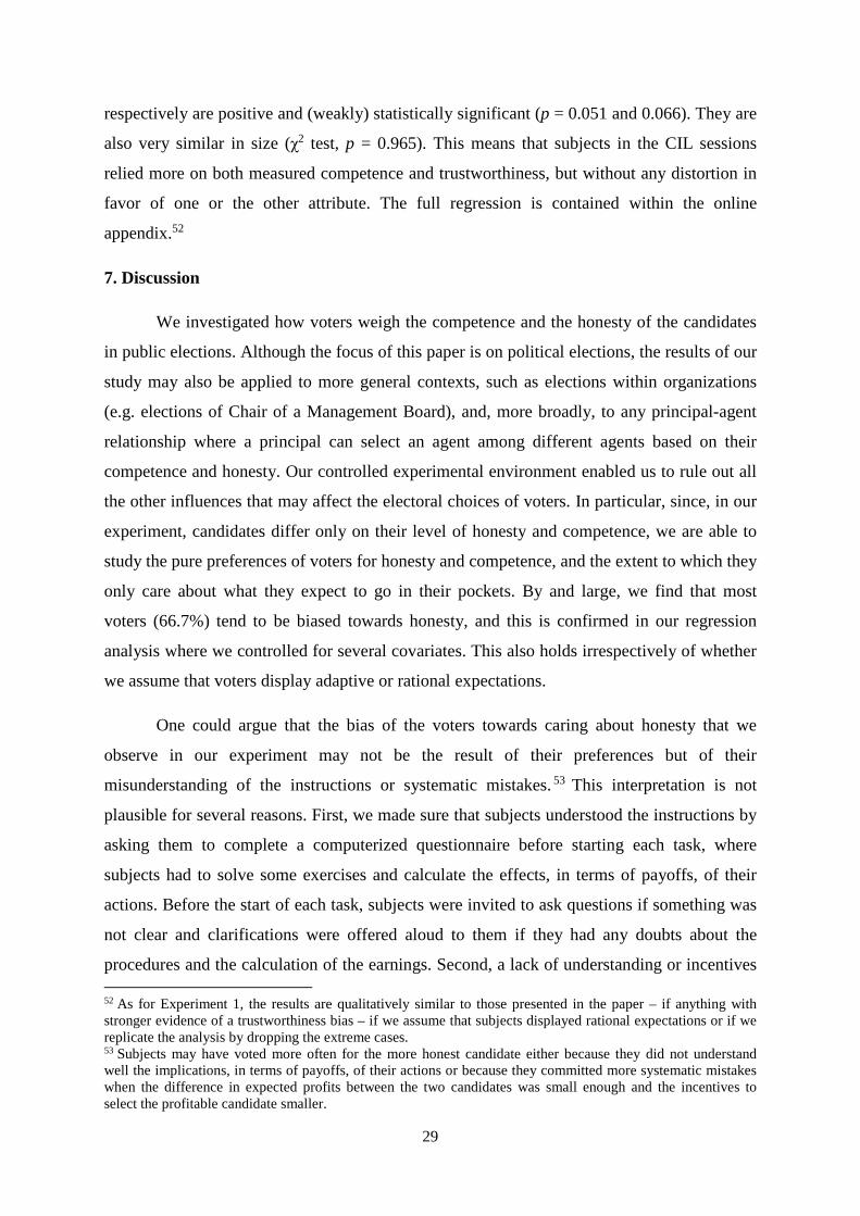
29

respectively are positive and (weakly) statistically significant (p = 0.051 and 0.066). They are

also very similar in size (χ2 test, p = 0.965). This means that subjects in the CIL sessions

relied more on both measured competence and trustworthiness, but without any distortion in

favor of one or the other attribute. The full regression is contained within the online

appendix.52

7. Discussion

We investigated how voters weigh the competence and the honesty of the candidates

in public elections. Although the focus of this paper is on political elections, the results of our

study may also be applied to more general contexts, such as elections within organizations

(e.g. elections of Chair of a Management Board), and, more broadly, to any principal-agent

relationship where a principal can select an agent among different agents based on their

competence and honesty. Our controlled experimental environment enabled us to rule out all

the other influences that may affect the electoral choices of voters. In particular, since, in our

experiment, candidates differ only on their level of honesty and competence, we are able to

study the pure preferences of voters for honesty and competence, and the extent to which they

only care about what they expect to go in their pockets. By and large, we find that most

voters (66.7%) tend to be biased towards honesty, and this is confirmed in our regression

analysis where we controlled for several covariates. This also holds irrespectively of whether

we assume that voters display adaptive or rational expectations.

One could argue that the bias of the voters towards caring about honesty that we

observe in our experiment may not be the result of their preferences but of their

misunderstanding of the instructions or systematic mistakes.53 This interpretation is not

plausible for several reasons. First, we made sure that subjects understood the instructions by

asking them to complete a computerized questionnaire before starting each task, where

subjects had to solve some exercises and calculate the effects, in terms of payoffs, of their

actions. Before the start of each task, subjects were invited to ask questions if something was

not clear and clarifications were offered aloud to them if they had any doubts about the

procedures and the calculation of the earnings. Second, a lack of understanding or incentives 52 As for Experiment 1, the results are qualitatively similar to those presented in the paper – if anything with stronger evidence of a trustworthiness bias – if we assume that subjects displayed rational expectations or if we replicate the analysis by dropping the extreme cases. 53 Subjects may have voted more often for the more honest candidate either because they did not understand well the implications, in terms of payoffs, of their actions or because they committed more systematic mistakes when the difference in expected profits between the two candidates was small enough and the incentives to select the profitable candidate smaller.

30

would have resulted in random mistakes in both directions. This however was not the case as

the bias occurred systematically in one direction. Third, in the data analysis, we controlled for

the behavior of those (few) inconsistent subjects who displayed a more random behavior and

could have failed to understand the instructions or taken the experiment less seriously.

Another possible criticism of our experiment is that subjects were provided only with

ex-ante measures of competence and honesty which, from the standpoint of the subjects, may

not necessarily capture the ex-post behavior of the public official. As a result, people may

have formed certain beliefs about the ex-post competence and honesty of the public official

which could have not reflected the information provided to them during the voting phase. We

are able to control for this possibility in four complementary ways. First, even if subjects

scaled up or down the information about the honesty of the candidates provided to them, this

does not change our results since the voting choice that brings the highest utility is the same

irrespectively of how utility is scaled (or the attributes are scaled).54 Second, we found a

significant correlation between early and later measures of honesty and competence which

would not justify such behavior unless subjects were extremely naïve. Third, we also

analyzed the data assuming that the subjects had correct beliefs and predictions of the future

behavior of the public official (rational expectations). Fourth, in the Belief treatment, we find

a significant and persistent bias towards honesty even when we base our analysis on the

elicited beliefs of the subjects.

Experiment 2 was conducted in France and the United Kingdom with subjects with a

variety of different backgrounds. It provides an acid test of the lower weight on competence

since there is only obviously an indirect link between the trustworthiness measure and the

honesty of the public official. It is therefore the more striking that we find a higher weight on

trustworthiness than competence in the French sample. The findings are more nuanced in the

54 This argument applies more generally every time a subject considers the information he or she receives about honesty and/or competence imprecise, and, as a result, he or she re-scales it. To illustrate this, suppose that a voter n believe that a unit of ex-ante honesty is equivalent to τ units of ex-post honesty. As long as this belief is the same for all the candidates (which is reasonable in our case since voters are only informed about the honesty and competence of the candidates and nothing else), the voting choice of the voter does not change. More formally, the probability that voter n chooses candidate i is the same irrespectively of how the attributes are scaled:

(�,) = (*+,#��,) > ��,�$ = (*+,#��,) − ��,� > 0$ = (*+,��∗�DE�)�����)�� − �∗#DE��������

�� > 0$ =

(*+,#�∗E�)����)

�� − �∗E�������

�� > 0$

In terms of our regression analysis, it means that the beliefs that change the scale of the attributes (honesty and competence), do not change the estimation of the parameters �� and ��.

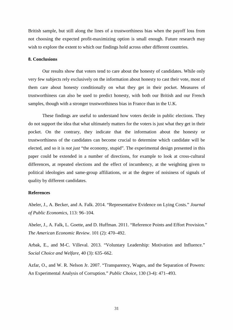
31

British sample, but still along the lines of a trustworthiness bias when the payoff loss from

not choosing the expected profit-maximizing option is small enough. Future research may

wish to explore the extent to which our findings hold across other different countries.

8. Conclusions

Our results show that voters tend to care about the honesty of candidates. While only

very few subjects rely exclusively on the information about honesty to cast their vote, most of

them care about honesty conditionally on what they get in their pocket. Measures of

trustworthiness can also be used to predict honesty, with both our British and our French

samples, though with a stronger trustworthiness bias in France than in the U.K.

These findings are useful to understand how voters decide in public elections. They

do not support the idea that what ultimately matters for the voters is just what they get in their

pocket. On the contrary, they indicate that the information about the honesty or

trustworthiness of the candidates can become crucial to determine which candidate will be

elected, and so it is not just “the economy, stupid”. The experimental design presented in this

paper could be extended in a number of directions, for example to look at cross-cultural

differences, at repeated elections and the effect of incumbency, at the weighting given to

political ideologies and same-group affiliations, or at the degree of noisiness of signals of

quality by different candidates.

References

Abeler, J., A. Becker, and A. Falk. 2014. “Representative Evidence on Lying Costs.” Journal

of Public Economics, 113: 96–104.

Abeler, J., A. Falk, L. Goette, and D. Huffman. 2011. “Reference Points and Effort Provision.”

The American Economic Review. 101 (2): 470–492.

Arbak, E., and M-C. Villeval. 2013. “Voluntary Leadership: Motivation and Influence.”

Social Choice and Welfare, 40 (3): 635–662.

Azfar, O., and W. R. Nelson Jr. 2007. “Transparency, Wages, and the Separation of Powers:

An Experimental Analysis of Corruption.” Public Choice, 130 (3-4): 471–493.

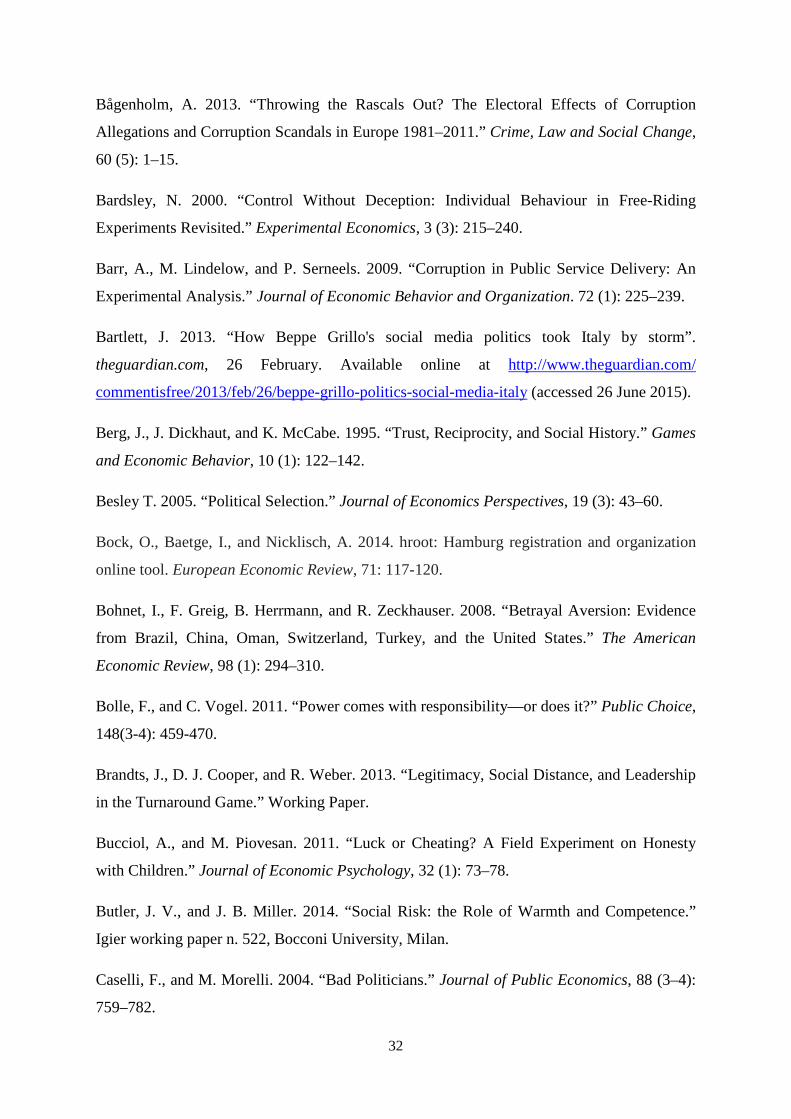
32

Bågenholm, A. 2013. “Throwing the Rascals Out? The Electoral Effects of Corruption

Allegations and Corruption Scandals in Europe 1981–2011.” Crime, Law and Social Change,

60 (5): 1–15.

Bardsley, N. 2000. “Control Without Deception: Individual Behaviour in Free-Riding

Experiments Revisited.” Experimental Economics, 3 (3): 215–240.

Barr, A., M. Lindelow, and P. Serneels. 2009. “Corruption in Public Service Delivery: An

Experimental Analysis.” Journal of Economic Behavior and Organization. 72 (1): 225–239.

Bartlett, J. 2013. “How Beppe Grillo's social media politics took Italy by storm”.

theguardian.com, 26 February. Available online at http://www.theguardian.com/

commentisfree/2013/feb/26/beppe-grillo-politics-social-media-italy (accessed 26 June 2015).

Berg, J., J. Dickhaut, and K. McCabe. 1995. “Trust, Reciprocity, and Social History.” Games

and Economic Behavior, 10 (1): 122–142.

Besley T. 2005. “Political Selection.” Journal of Economics Perspectives, 19 (3): 43–60.

Bock, O., Baetge, I., and Nicklisch, A. 2014. hroot: Hamburg registration and organization

online tool. European Economic Review, 71: 117-120.

Bohnet, I., F. Greig, B. Herrmann, and R. Zeckhauser. 2008. “Betrayal Aversion: Evidence

from Brazil, China, Oman, Switzerland, Turkey, and the United States.” The American

Economic Review, 98 (1): 294–310.

Bolle, F., and C. Vogel. 2011. “Power comes with responsibility—or does it?” Public Choice,

148(3-4): 459-470.

Brandts, J., D. J. Cooper, and R. Weber. 2013. “Legitimacy, Social Distance, and Leadership

in the Turnaround Game.” Working Paper.

Bucciol, A., and M. Piovesan. 2011. “Luck or Cheating? A Field Experiment on Honesty

with Children.” Journal of Economic Psychology, 32 (1): 73–78.

Butler, J. V., and J. B. Miller. 2014. “Social Risk: the Role of Warmth and Competence.”

Igier working paper n. 522, Bocconi University, Milan.

Caselli, F., and M. Morelli. 2004. “Bad Politicians.” Journal of Public Economics, 88 (3–4):

759–782.

33

Christie, R., F. L. Geis, and D. Berger. 1970. Studies in Machiavellianism. New York:

Academic Press.

Croson, R. T. A. 2005. “Deception in Economics Experiments.” In C. Gerschlager (Ed.),

Deception in Markets: An Economic Analysis, Basingstoke: Palgrave Macmillan.

DeMaio, T. J. 1984. Social Desirability and Survey Measurement: A Review. New York:

Russell Sage Foundation.

Eckel, C. C., P. J. Grossman, C. A. Johnson, A. C. M. de Oliveira, C. Rojas, and R. K.

Wilson. 2012. “School Environment and Risk Preferences: Experimental Evidence.” Journal

of Risk and Uncertainty, 45 (3): 265–292.

Eggers, A., and A. C. Fisher. 2011. “Electoral Accountability and the UK Parliamentary

Expenses Scandal: Did Voters Punish Corrupt MPs?” SSRN Scholarly Paper ID 1931868.

Ferraz, C., and F. Finan. 2008. “Exposing Corrupt Politicians: The Effects of Brazil’s

Publicly Released Audits on Electoral Outcomes.” The Quarterly Journal of Economics, 123

(2): 703–745.

Fischbacher, U. 2007. “z-Tree: Zurich Toolbox for Ready-made Economic Experiments.”

Experimental Economics, 10 (2): 171–178.

Fischbacher, U., and F. Föllmi-Heusi. 2013. “Lies in Disguise-an Experimental Study on

Cheating.” Journal of the European Economic Association, 11 (3): 525–547.Fiske, S. T., A. J.

Cuddy, and P. Glick. 2007. “Universal dimensions of social cognition: warmth and

competence.” Trends in Cognitive Sciences, 11, 77-83.

Fiske, S. T., A. J. Cuddy, P. Glick, and J. Xu. 2002. “A Model of (Often Mixed) Stereotype

Content: Competence and Warmth Respectively Follow From Perceived Status and

Competition.” Journal of Personality and Social Psychology, 82, 878-902.

Gächter, S., and E. Renner. 2005. “Leading by Example in the Presence of Free Rider

Incentives.” CeDEx Discussion Paper, University of Nottingham.

Gächter, S., D. Nosenzo, E. Renner, and M. Sefton. 2012. “Who Makes a Good Leader?

Cooperativeness, Optimism, and Leading-by-Example.” Economic Inquiry, 50 (4): 953–967.

34

Galeotti, F., and D. J. Zizzo. 2014. “Competence versus Trustworthiness: What Do Voters

Care About?” University of East Anglia Applied and Financial Economics Working Paper

Series 060, School of Economics, University of East Anglia, Norwich, UK.

Gneezy, U. 2005. “Deception: The Role of Consequences.” The American Economic Review,

95 (1): 384–394.

Güth, W., M. V. Levati, M. Sutter, and E. van der Heijden. 2007. “Leading by Example with

and Without Exclusion Power in Voluntary Contribution Experiments.” Journal of Public

Economics, 91 (5–6): 1023–1042.

Hamman, J. R., R. A. Weber, and J. Woon. 2011. “An Experimental Investigation of

Electoral Delegation and the Provision of Public Goods.” American Journal of Political

Science, 55 (4): 738–752.

Hao, L., and D. Houser. 2013. “Perceptions, Intentions, and Cheating”. Working Paper 1039,

George Mason University, Interdisciplinary Center for Economic Science.

Houser, D., S. Vetter, and J. Winter. 2012. “Fairness and Cheating.” European Economic

Review, 56 (8): 1645–1655.

Kocher, M. G., G. Pogrebna, and M. Sutter. 2013. “Other-regarding Preferences and

Management Styles.” Journal of Economic Behavior and Organization, 88: 109–132.

Kulisheck, M. R, and J. J Mondak. 1996. “Candidate Quality and the Congressional Vote: A

Causal Connection?” Electoral Studies, 15 (2): 237–253.

Kumru, C. S., and L. Vesterlund. 2010. “The Effect of Status on Charitable Giving.” Journal

of Public Economic Theory, 12 (4): 709–735.

Levy, D. M., K. Padgitt, S. J. Peart, D. Houser, and E. Xiao. 2011. “Leadership, Cheap Talk

and Really Cheap Talk.” Journal of Economic Behavior and Organization, 77 (1): 40–52.

Lodge, M., P. Stroh, and J. Wahlke. 1990. “Black-box Models of Candidate Evaluation.”

Political Behavior, 12 (1): 5–18.

Marquardt, D.W., 1980. “You Should Standardize the Predictor Variables in Your Regression

Models.” Journal of the American Statistical Association, 75 (369): 87-91.

35

Mas-Colell, A., M. D. Whinston, and J. R. Green. 1995. Microeconomic theory. Vol. 1. New

York: Oxford university press.

Mazar, N., and D. Ariely. 2006. “Dishonesty in Everyday Life and Its Policy Implications.”

Journal of Public Policy and Marketing, 25 (1): 117–126.

McCurley, C., and J. J. Mondak. 1995. “Inspected by #1184063113: The Influence of

Incumbents’ Competence and Integrity in U.S. House Elections.” American Journal of

Political Science, 39 (4): 864.

Messick, D. M., H. Wilke, M. B. Brewer, R. M. Kramer, P. E. Zemke, and L. Lui. 1983.

“Individual Adaptations and Structural Change as Solutions to Social Dilemmas.” Journal of

Personality and Social Psychology, 44 (2): 294–309.

Mondak, J. J. 1995. “Competence, Integrity, and the Electoral Success of Congressional

Incumbents.” The Journal of Politics, 57 (04): 1043–1069.

Mondak, J. J., and R. Huckfeldt. 2006. “The Accessibility and Utility of Candidate Character

in Electoral Decision Making.” Electoral Studies, 25 (1): 20–34.

Moxnes, E., and E. van der Heijden. 2003. “The Effect of Leadership in a Public Bad

Experiment.” Journal of Conflict Resolution, 47 (6): 773–795.

Otto, P. E., and F. Bolle. 2013. “The Advantage of Hierarchy: Inducing Responsibility and

Selecting Ability?” Available at SSRN 2327491.

Peters, J. G., and S. Welch. 1980. “The Effects of Charges of Corruption on Voting Behavior

in Congressional Elections.” The American Political Science Review, 74 (3): 697.

Pokorny, K. 2008. “Pay—but Do Not Pay Too Much: An Experimental Study on the Impact

of Incentives.” Journal of Economic Behavior and Organization, 66 (2): 251–264.

Potters, J., M. Sefton, and L. Vesterlund. 2007. “Leading-by-example and Signaling in

Voluntary Contribution Games: An Experimental Study.” Economic Theory, 33 (1): 169–182.

Rabin, M. 1993. “Incorporating Fairness into Game Theory and Economics.” The American

Economic Review, 83 (5): 1281–1302.

Rivas, M. F., and M. Sutter. 2011. “The Benefits of Voluntary Leadership in Experimental

Public Goods Games.” Economics Letters, 112 (2): 176–178.

36

Samuelson, C. D, and D. M. Messick. 1986. “Alternative Structural Solutions to Resource

Dilemmas.” Organizational Behavior and Human Decision Processes, 37 (1): 139–155.

Samuelson, C. D., D. M. Messick, C. Rutte, and H. Wilke. 1984. “Individual and Structural

Solutions to Resource Dilemmas in Two Cultures.” Journal of Personality and Social

Psychology, 47 (1): 94–104.

Shampanier, K., N. Mazar, and D. Ariely. 2007. “Zero as a Special Price: The True Value of

Free Products.” Marketing Science, 26 (6): 742–757.

Stöber, J. 2001. “The Social Desirability Scale-17 (SDS-17): Convergent Validity,

Discriminant Validity, and Relationship with Age.” European Journal of Psychological

Assessment, 17 (3): 222–232.

Sutter, M. 2009. “Deception Through Telling the Truth?! Experimental Evidence From

Individuals and Teams.” The Economic Journal, 119 (534): 47–60.

Welch, S., and J. R. Hibbing. 1997. “The Effects of Charges of Corruption on Voting

Behavior in Congressional Elections, 1982–1990.” The Journal of Politics, 59 (01): 226–239.

Winters, M. S., and R. Weitz-Shapiro. 2013. “Lacking Information or Condoning Corruption:

When Do Voters Support Corrupt Politicians?” Comparative Politics, 45 (4): 418–436.

37

Figures and Tables

Figure 1: Probability that a candidate i is elected

Notes: P(i) is the probability of electing a candidate i in election k. This is computed using a locally weighted linear regression on the dichotomous variable taking value 1 when the candidate i is elected and 0 otherwise. “Delta C” is the difference in standardized competence between candidate i and candidate j in the situation (election) k. “Delta H” is the difference in standardized honesty between candidate i and candidate j in the situation (election) k. The standardized values are obtained by subtracting the mean and dividing by the standard deviation. Each smoothed value of the locally weighted surface is computed using neighboring data points defined within the span of 0.6 (60% of the data).

Azimuthal direction: 320° Azimuthal direction: 0°

Azimuthal direction: 90°

38

Figure 2: Probability of electing the more honest candidate

Notes: P(T) is the probability of electing the more honest candidate. ∆π is the difference in expected payoffs between the more and less honest candidate. The running means are weighted to give more importance to near points than far, and computed using a bandwith of 0.6 (60% of the data). The data correspond to cases where there was a trade-off between honesty and competence.

0.1

.2.3

.4.5

.6.7

.8.9

1P

(H)

-50 -45 -40 -35 -30 -25 -20 -15 -10 -5 0 5 10 15 20 25 30 35 40 45 50 ∆π = π(H) - π(C)

No Belief treatment

0.1

.2.3

.4.5

.6.7

.8.9

1P

(H)

-50 -45 -40 -35 -30 -25 -20 -15 -10 -5 0 5 10 15 20 25 30 35 40 45 50 ∆π = π(H) - π(C)

(based on actual information)Belief treatment

0.1

.2.3

.4.5

.6.7

.8.9

1P

(H)

-50 -45 -40 -35 -30 -25 -20 -15 -10 -5 0 5 10 15 20 25 30 35 40 45 50 ∆π = π(H) - π(C)

(based on beliefs)Belief treatment

0.1

.2.3

.4.5

.6.7

.8.9

1P

(H)

-50 -45 -40 -35 -30 -25 -20 -15 -10 -5 0 5 10 15 20 25 30 35 40 45 50 ∆π = π(H) - π(C)

(based on actual information)All treatments

Smoothed means (All subjects) Theoretical prediction

Smoothed means (No inconsistent)

39

Figure 3: Proportion of cases where the less profitable candidate was voted

Notes: The orange bar identifies the proportion of cases where the voters elected the more honest candidate when the latter was the less profitable one. The blue bar identifies the proportion of cases where the voters elected the more competent candidate when the latter was the less profitable one. The intervals in the x-axis are in experimental points. The data correspond to cases where there was a trade-off between honesty and competence. We omit cases of perfect profit equality, one from the No Belief treatment (100% of votes to the more honest candidate), and seven from the Belief treatment based on beliefs (71.43% of votes to the more honest candidate). Stars identify the significance level of Wilcoxon signed-rank tests where the unit of observation is the average vote (calculated as the mean of a binary variable which is equal to 1 if the candidate was voted, and 0 otherwise) casted for the less profitable and more competent candidate, and the less profitable and more honest candidate respectively. * p < 0.1, ** p < 0.05, *** p < 0.01, NA = p-value not available due to small number of independent observations.

40

Figure 4: Probability of electing the more honest candidate (Experiment 2)

Notes: P(T) is the probability of electing the more honest candidate. ∆π is the difference in expected payoffs between the more and less trustworthy candidate. The running means are weighted to give more importance to near points than far, and computed using a bandwith of 0.6 (60% of the data). The data correspond to cases where there was a trade-off between trustworthiness and competence.

0.1

.2.3

.4.5

.6.7

.8.9

1P

(T)

-40 -35 -30 -25 -20 -15 -10 -5 0 5 10 15 20 25 30 35 40 ∆π = π(T) - π(C)

Smoothed means (UK subjects) Theoretical prediction

Smoothed means (France subjects)

41

Table 1: Competence and Honesty

Competence Honesty

Mean St. Dev. Mean St. Dev.

Stage 1 40.17 15.83 0.45 0.30

Stage 2 51.44 17.80 0.39 0.28

Table 2: Voting choices

Treatment Situation Honesty Competence Votes for i Votes for j Tot.

No Belief

Strict or weak dominance

Ti ≥ Tj Ti > Tj

Ci > Cj Ci ≥ Cj

114 (98.28%)

2 (1.72%)

116 (100%)

Trade-off Ti > Tj Ci < Cj 196

(58.68%) 138

(41.32%) 334

(100%) Equality Ti = Tj Ci = Cj . . .

Belief (based on actual

information)

Strict or weak dominance

Ti ≥ Tj Ti > Tj

Ci > Cj Ci ≥ Cj

97 (92.38%)

8 (7.62%)

105 (100%)

Trade-off Ti > Tj Ci < Cj 161

(48.35%) 172

(51.65%) 333

(100%) Equality Ti = Tj Ci = Cj . . .

Total

Strict or weak dominance

Ti ≥ Tj Ti > Tj

Ci > Cj Ci ≥ Cj

211 (95.48%)

10 (4.52%)

221 (100%)

Trade-off Ti > Tj Ci < Cj 357

(53.52%) 310

(46.48%) 667

(100%)

Belief (based on

subjects’ beliefs)

Strict or weak dominance

Ti ≥ Tj Ti > Tj

Ci > Cj Ci ≥ Cj

155 (90.64%)

16 (9.36%)

171 (100%)

Trade-off Ti > Tj Ci < Cj 140

(53.23%) 123

(46.77%) 263

(100%)

Equality Ti = Tj Ci = Cj 4

(100%) 0

(0%) 4

(100%)

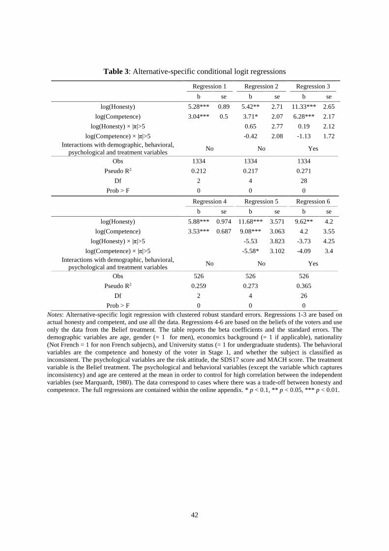
42

Table 3: Alternative-specific conditional logit regressions

Regression 1 Regression 2 Regression 3

b se b se b se

log(Honesty) 5.28*** 0.89 5.42** 2.71 11.33*** 2.65

log(Competence) 3.04*** 0.5 3.71* 2.07 6.28*** 2.17

log(Honesty) × |π|>5

0.65 2.77 0.19 2.12

log(Competence) × |π|>5

-0.42 2.08 -1.13 1.72 Interactions with demographic, behavioral,

psychological and treatment variables No No Yes

Obs 1334

1334

1334

Pseudo R2 0.212

0.217

0.271

Df 2

4

28

Prob > F 0

0

0

Regression 4 Regression 5 Regression 6

b se b se b se

log(Honesty) 5.88*** 0.974 11.68*** 3.571 9.62** 4.2

log(Competence) 3.53*** 0.687 9.08*** 3.063 4.2 3.55

log(Honesty) × |π|>5 -5.53 3.823 -3.73 4.25

log(Competence) × |π|>5 -5.58* 3.102 -4.09 3.4 Interactions with demographic, behavioral,

psychological and treatment variables No No Yes

Obs 526 526 526

Pseudo R2 0.259 0.273 0.365

Df 2 4 26

Prob > F 0 0 0 Notes: Alternative-specific logit regression with clustered robust standard errors. Regressions 1-3 are based on actual honesty and competent, and use all the data. Regressions 4-6 are based on the beliefs of the voters and use only the data from the Belief treatment. The table reports the beta coefficients and the standard errors. The demographic variables are age, gender (= 1 for men), economics background (= 1 if applicable), nationality (Not French = 1 for non French subjects), and University status (= 1 for undergraduate students). The behavioral variables are the competence and honesty of the voter in Stage 1, and whether the subject is classified as inconsistent. The psychological variables are the risk attitude, the SDS17 score and MACH score. The treatment variable is the Belief treatment. The psychological and behavioral variables (except the variable which captures inconsistency) and age are centered at the mean in order to control for high correlation between the independent variables (see Marquardt, 1980). The data correspond to cases where there was a trade-off between honesty and competence. The full regressions are contained within the online appendix. * p < 0.1, ** p < 0.05, *** p < 0.01.

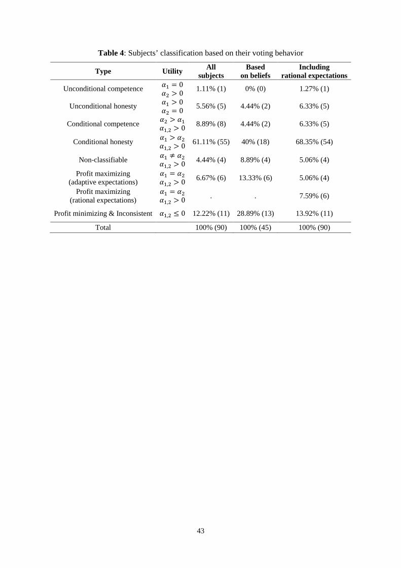
43

Table 4: Subjects’ classification based on their voting behavior

Type Utility All subjects

Based on beliefs

Including rational expectations

Unconditional competence �� = 0 �� > 0

1.11% (1) 0% (0) 1.27% (1)

Unconditional honesty �� > 0 �� = 0

5.56% (5) 4.44% (2) 6.33% (5)

Conditional competence �� > �� ��,� > 0

8.89% (8) 4.44% (2) 6.33% (5)

Conditional honesty �� > �� ��,� > 0

61.11% (55) 40% (18) 68.35% (54)

Non-classifiable �� ≠ �� ��,� > 0

4.44% (4) 8.89% (4) 5.06% (4)

Profit maximizing (adaptive expectations)

�� = �� ��,� > 0

6.67% (6) 13.33% (6) 5.06% (4)

Profit maximizing (rational expectations)

�� = �� ��,� > 0

. . 7.59% (6)

Profit minimizing & Inconsistent ��,� ≤ 0 12.22% (11) 28.89% (13) 13.92% (11)

Total 100% (90) 100% (45) 100% (90)

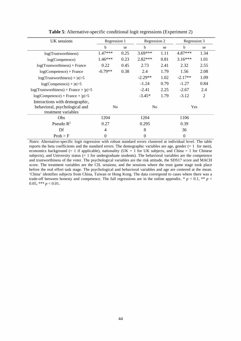
44

Table 5: Alternative-specific conditional logit regressions (Experiment 2)

UK sessions Regression 1 Regression 2 Regression 3

b se b se b se

log(Trustworthiness) 1.47*** 0.25 3.69*** 1.11 4.87*** 1.34

log(Competence) 1.46*** 0.23 2.82*** 0.81 3.16*** 1.01 log(Trustworthiness) × France 0.22 0.45 2.73 2.41 2.32 2.55

log(Competence) × France -0.79** 0.38 2.4 1.79 1.56 2.08

log(Trustworthiness) × |π|>5 -2.29** 1.02 -2.17** 1.09

log(Competence) × |π|>5 -1.24 0.79 -1.27 0.84 log(Trustworthiness) × France × |p|>5 -2.41 2.25 -2.67 2.4

log(Competence) × France × |p|>5 -3.45* 1.79 -3.12 2 Interactions with demographic, behavioral, psychological and

treatment variables No No Yes

Obs 1204

1204

1106 Pseudo R2 0.27

0.295

0.39

Df 4

8

36 Prob > F 0

0

0

Notes: Alternative-specific logit regression with robust standard errors clustered at individual level. The table reports the beta coefficients and the standard errors. The demographic variables are age, gender (= 1 for men), economics background (= 1 if applicable), nationality (UK = 1 for UK subjects, and China = 1 for Chinese subjects), and University status (= 1 for undergraduate students). The behavioral variables are the competence and trustworthiness of the voter. The psychological variables are the risk attitude, the SDS17 score and MACH score. The treatment variables are the CIL sessions, and the sessions where the trust game stage took place before the real effort task stage. The psychological and behavioral variables and age are centered at the mean. ‘China’ identifies subjects from China, Taiwan or Hong Kong. The data correspond to cases where there was a trade-off between honesty and competence. The full regressions are in the online appendix. * p < 0.1, ** p < 0.05, *** p < 0.01.

1

Competence versus Honesty: What Do Voters Care About?

By Fabio Galeotti and Daniel John Zizzo

Online Appendix

A. Experimental instructions

B. Final questionnaire

C. Background information on participants

D. Full regressions of Tables 4 and 5

E. Analysis with rational expectations

F. Analysis without outliers

A. Experimental instructions A.1 Experiment 1 (instructions are translated from French)

Instructions

Introduction

This is an experiment on decision making. The instructions are the same for all participants. During the experiment, you are not allowed to communicate with other participants. Please raise your hand if you have any questions at any point during the experiment. If you have any questions, the experimenter will come to you and answer your questions privately. If the question is relevant to everyone, the experimenter will repeat the answer aloud.

The experiment consists of two stages. In addition to these two stages, you will be asked some individual questions at the end of the experiment. At the beginning of each stage you will receive the corresponding instructions. The information you provide in each stage of the experiment may be reported to other participants at later stages of the experiment. However, all of your decisions and answers will remain anonymous.

During this experiment, your earnings depend on your decisions and the decisions of the other participants. It is therefore important that you read the instructions with care. Your earnings from the experiment will be computed in “points”.

At the end of the experiment one stage will be chosen at random, and you will be paid the points that you earned in that stage. The points that you earn in that stage will be converted into euros at an exchange rate of 1 point = 20 cents. In addition to this, you will also be paid a show-up fee of 5 euros and any additional earnings that you may obtain by answering the questions at the end of the experiment. You will be paid individually and in cash in a separate room by a person who is not present during the experiment and who is not aware of the content of this experiment.

2

First stage

In this stage of the experiment, you will be matched at random with two other participants. You will never interact with these persons again in the remainder of the experiment. You and these two participants will be referred to as co-participants. The three of you will have a common fund. At the beginning of the task, the value of the common fund will be set to 0 points.

Every co-participant will individually work on a task. The task is to count the number of 1s in a series of tables containing 0s and 1s. The figure shows the kind of screen you will see later:

You will have to enter the number of 1s into the box below the table and click the Submit button. After you have submitted your answer, a new table will be generated. You will have 10 minutes to complete this task. Your remaining time will be displayed in the upper right hand corner of the screen.

Only one co-participant’s work will count for the earnings of this stage of the experiment. This co-participant will be referred to as the appointed co-participant. After the appointed co-participant correctly solves 40 tables, each additional correct answer of the appointed co-participant will increase the value of the common fund by 4 points. The greater the number of tables the appointed co-participant solves correctly over and above the first 40 correctly solved tables, the larger the value of the common fund will be.

At the end of the task, the common fund will have accumulated a certain number of points equal to four times the number of tables that the appointed co-participant correctly solved on top of the first 40 correctly solved tables. Only the appointed co-participant will know the number of tables that he or she correctly solved (and so the value of the common fund). He or she will be asked to report the value of the common fund to the other co-participants. He or she can report any number between a minimum value of 10% and the true value of the common

3

fund. This number corresponds to the reported value of the common fund. The reported value of the common fund will be split equally between the co-participants. That is, each co-participant (including the appointed co-participant) will receive 1/3 of the reported value of the common fund. If applicable, the appointed co-participant will also earn the whole of the non-reported value of the common fund, that is the value of the common fund not reported. Note that the appointed co-participant will be free to report or not the true value of the common fund. Moreover, the other co-participants will only be informed of the reported value of the common fund.

Example: Suppose the appointed co-participant solves 52 tables correctly (hence 12 tables over and above 40 correctly solved tables); the value of the common fund is 12 × 4 = 48. The appointed co-participant however reports a value of 33. The non-reported value of the common fund is 48 – 33 = 15. The earnings are therefore:

• 33 / 3 = 11 for each non-appointed co-participant;

• 33 / 3 + 15 = 26 for the appointed co-participant.

How is the appointed co-participant selected? The computer will randomly assign the role of appointed co-participant to one of the three co-participants. Each co-participant will be informed whether he or she is or not the appointed co-participant only at the end of the experiment. Hence, at this stage, every co-participant will have to solve tables and make a decision as if he or she were the appointed co-participant.

The results and earnings for this stage will be communicated to you at the end of the experiment and will depend on whether you have been assigned the role of appointed co-participant or not. If you are not assigned the role of appointed co-participant, your work and decision will be ignored; if you are assigned the role of appointed co-participant, your work and decision will determine your and other co-participants’ earnings for this stage.

In summary

• You will be randomly matched with two other participants you will never interact with in the remainder of the experiment. You and these two participants will be referred to as co-participants. The three of you will have a common fund with an initial value of 0 points.

• The computer will randomly assign to one of you the role of appointed co-participant. Each co-participant will be informed whether he or she is or not the appointed co-participant only at the end of the experiment. Hence, at this stage, everyone will work and make a decision as if he or she were the appointed co-participant.

• Everyone will work for 10 minutes on the task which consists in counting 1s in a series of tables containing 0s and 1s. If a co-participant is assigned the role of appointed co-participant, for each table that he or she correctly solves on top of the first 40 correctly solved tables, the value of the common fund increases by 4 points.

• At the end of the task each co-participant will be asked to report any number between a minimum value of 10% and the total value of the common fund generated by his or

4

her work in case he or she were to be assigned the role of appointed co-participant. If the co-participant is indeed the appointed co-participant, this number constitutes the reported value of the common fund. At the end of the experiment, the other co-participants will be informed only about the reported value of the common fund.

• The reported value of the common fund will be divided in equal parts (each worth 1/3 of the reported value) between the co-participants (including the appointed co-participant). If applicable, the appointed co-participant will also earn the whole of the non-reported value of the common fund, that is the value of common fund not reported.

Second stage

In this stage, you will be randomly matched with two other participants you have never been matched with before. As in the first stage, you and these two participants will be referred to as co-participants. This second stage is identical to the first one except for the selection of the appointed co-participant.

How is the appointed co-participant selected in the second stage? Before starting the task of counting 1s in a series of tables, each co-participant will be placed in 10 situations. Only one of these will be real, the others will be fictional.

In each situation, each co-participant will be informed of:

• the number of tables correctly solved by each other co-participant in the first stage of the experiment;

• the proportion of the common fund that each other co-participant reported in the first stage of the experiment if he or she were to be the appointed co-participant in that stage.

However, only in the real situation, the information provided is about your actual current co-participants. In the fictional situations, the information provided is about people who participated in past sessions of this experiment.

For each situation, each co-participant will be asked to choose which of the two other co-participants he or she would like to select as the appointed co-participant for this second stage. Only the decision of one randomly selected co-participant in the real situation will be implemented and count towards your earnings of this stage. Note that, for all you know, each situation could be the real one, in which case ALL information you are given about it is true, and only the real one may have any effect on who is going to be the appointed co-participant in this second stage. Hence, it is in your best interest to treat each situation as if it is real and to choose, for each situation, the co-participant that you really want as the appointed co-participant in this second stage.

Then the task of counting 1s in a series of tables will start. At the end of the experiment, the computer will inform each co-participant whether or not he or she is the appointed co-participant for this second stage based on the outcome of the real situation.

{In squared parenthesis, part included only in BELIEF treatment}

5

[Guesses. For each situation, before you choose who you want to select as the appointed co-participant for this second stage, you will also be asked to indicate how many tables you think each co-participant will correctly solve, and what proportion of the common fund you think each co-participant will report at the end of the task. At the end of the experiment, the computer will randomly draw one of your two guesses about one of your co-participants in the real situation (i.e. tables correctly solved or proportion of the common fund reported).

You will be paid for this randomly drawn guess as follows:

• If your guess is correct, you will earn an extra 2 euros; • if your guess is incorrect by 1 table (in the case the randomly drawn guess is about the

tables correctly solved) or 1 percentage point (in the case the randomly drawn guess is about the proportion of the common fund reported) respectively, you will earn 1 euro and 90 cents;

• if your guess is incorrect by 2 tables or 2 percentage points respectively, you will earn 1 euro and 80 cents;

• if your guess is incorrect by 3 tables or 3 percentage points respectively, you will earn 1 euros and 70 cents, and so on: you earn 10 cents less for each additional table or percentage point by which you are incorrect;

• if your guess is incorrect by a number of tables or percentage points respectively greater than or equal to 20, you will earn 0 euros.]

In summary

• You will be randomly matched with two other participants you have never been matched with before. You and these two participants will be referred to as co-participants. The three of you will have a common fund with an initial value of 0 points.

• Each co-participant will choose whom he or she wants to select as appointed co-participant for this second stage between the other two co-participants in different situations. Only one of these situations is the real one. The decision of one co-participant selected at random in the real situation will be implemented. Each co-participant will be informed whether he or she is or not the appointed co-participant for this second stage only at the end of the experiment. Hence, at this stage, everyone will work and make a decision as if he or she were the appointed co-participant for this stage.

• Everyone will work for 10 minutes on the task which consists in counting 1s in a series of tables containing 0s and 1s. If a co-participant is assigned the role of appointed co-participant for this second stage, for each table that he or she correctly solves on top of the first 40 correctly solved tables, the value of the common fund increases by 4 points.

• At the end of the task each co-participant will be asked to report any number between a minimum value of 10% and the total value of the common fund generated by his or her work in case he or she were to be assigned the role of appointed co-participant for this second stage. If the co-participant is indeed the appointed co-participant for this second stage, this number constitutes the reported value of the common fund. At the end of the experiment, the other co-participants will be informed only about the reported value of the common fund.

6

• The reported value of the common fund will be divided in equal parts (each worth 1/3 of the reported value) between the co-participants (including the appointed co-participant for this second stage). If applicable, the appointed co-participant for this second stage will also earn the whole of the non-reported value of the common fund, that is the value of common fund not reported.

7

A.2 Experiment 2

• Baseline (in half of the sessions, the order of stage 1 and stage 2 was inverted)

Instructions

Introduction

This is an experiment on decision making. The instructions are the same for all participants. During the experiment, you are not allowed to communicate with other participants. Please raise your hand if you have any questions at any point during the experiment. If you have any questions, the experimenter will come to you and answer your questions privately. If the question is relevant to everyone, the experimenter will repeat the answer aloud.

The experiment consists of three stages. In addition to these three stages, you will be asked some individual questions at the end of the experiment. At the beginning of each stage you will receive the corresponding instructions. The information you provide in each stage of the experiment may be reported to other participants at later stages of the experiment. However, all of your decisions and answers will remain anonymous.

During this experiment, your earnings depend on your decisions and the decisions of the other participants. It is therefore important that you read the instructions with care. Your earnings from the experiment will be computed in “points”.

At the end of the experiment one stage will be chosen at random, and you will be paid the points that you earned in that stage. The points that you earn in that stage will be converted into pounds at an exchange rate of 1 point = 20 pence. In addition to this, you will also be paid a show-up fee of 2 pounds and any additional earnings that you may obtain by answering the questions at the end of the experiment. You will be paid individually and in cash in a separate room by a person who is not present during the experiment and who is not aware of the content of this experiment.

First stage

In this stage of the experiment your task will be to count the number of 1s in a series of tables containing 0s and 1s. The figure shows the kind of screen you will see later:

8

You will have to enter the number of 1s into the box below the table and click the Submit button. After you have submitted your answer, a new table will be generated.

You will only earn money after correctly solving 40 tables. Specifically, you will receive 1 point for each table you correctly solve on top of the first 40 correctly solved tables. The greater the number of tables you solve correctly over and above the first 40 correctly solved tables, the more points you will earn.

You will have 10 minutes to complete the first stage of the experiment. Your remaining time will be displayed in the upper right hand corner of the screen.

Second stage

In this stage of the experiment, you will be matched at random with another participant. You will never interact with this person again in the remainder of the experiment. One of the two will be randomly assigned the role of participant A, and the other the role of participant B.

Participant A will receive an endowment of 30 points. He or she will decide whether or not to transfer all the 30 points to participant B. There are two scenarios:

1. If participant A decides not to transfer the 30 points to participant B, participant A will earn 30 points and participant B 0 points.

2. If participant A decides to transfer the 30 points to participant B, these points get multiplied by 3 before they are received by participant B. Hence, participant B will receive 90 points overall. Participant B then will decide how many points to keep and how many points to return to participant A. Specifically, he/she can return to participant A any amount between a minimum of 9 points to a maximum of 90 points.

9

You will be informed about your role (participant A or B) only at the end of the experiment. Hence, at this stage, you will have to make decisions in the roles of both participant A and participant B:

• As participant A, you will have to decide if you want to transfer the 30 points or not to participant B.

• As participant B, you will make a decision without knowing if participant A has chosen to transfer or not the 30 points to you. Specifically, you will have to decide how many points you would wish to return to participant A if participant A were to transfer his or her 30 points to you.

At the end of this stage, if participant A has chosen not to transfer the 30 points, participant B’s decision will be ignored and earnings will be 30 points for participant A and 0 for participant B. If participant A has chosen to transfer the 30 points, participant B’s decision will determine the earnings of both participants.

The results and earnings for this stage will be communicated to you at the end of the experiment and will depend on the role that you have been assigned to.

Third stage

The task in this stage of the experiment is to count 1s in a series of tables as in the first stage of the experiment. However, new rules are now in effect, which did not apply in the first stage.

Specifically, you will be randomly matched with two other participants you have never been matched with before. You and these two participants will now be referred to as co-participants. The three of you will have a common fund. At the beginning of the task, the value of the common fund will be set to 0 points. Every co-participant will individually work on the task for 10 minutes (the remaining time will be displayed in the upper right hand corner of the work screen). However, only one co-participant’s work will count for the earnings of this stage of the experiment. This co-participant will be referred to as the appointed co-participant. After the appointed co-participant correctly solves 40 tables, each additional correct answer of the appointed co-participant will increase the value of the common fund by 4 points.

At the end of the task, the common fund will have accumulated a certain number of points equal to four times the number of tables that the appointed co-participant correctly solved on top of the first 40 correctly solved tables. Only the appointed co-participant will know the number of tables that he or she correctly solved (and so the value of the common fund). He or she will be asked to report the value of the common fund to the other co-participants. He or she can report any number between 0 and the true value of the common fund. This number corresponds to the reported value of the common fund. The reported value of the common fund will be split equally between the co-participants. That is, each co-participant (including the appointed co-participant) will receive 1/3 of the reported value of the common fund. If applicable, the appointed co-participant will also earn the whole of the non-reported value of the common fund, that is the value of the common fund not reported. Note that the appointed

10

co-participant will be free to report or not the true value of the common fund. Moreover, the other co-participants will only be informed of the reported value of the common fund.

Example: Suppose the appointed co-participant solves 52 tables correctly (hence 12 tables over and above 40 correctly solved tables); the value of the common fund is 12 × 4 = 48. The appointed co-participant however reports a value of 33. The non-reported value of the common fund is 48 – 33 = 15. The earnings are therefore:

• 33 / 3 = 11 for each non-appointed co-participant;

• 33 / 3 + 15 = 26 for the appointed co-participant.

How is the appointed co-participant selected? Before starting the task, each co-participant will be informed of:

• the number of tables correctly solved by each other co-participant in the first stage of the experiment where the task was to count 1s in tables;

• the proportion of points that each other co-participant in the role of participant B returned to participant A in the second stage of the experiment.

Each co-participant will then be asked to choose which of the two other co-participants he or she would like to select as the appointed co-participant. The decision of one randomly selected co-participant will be implemented. Hence, it is in your best interest to choose the co-participant that you really want as the appointed co-participant.

Afterwards, the computer will inform each co-participant whether or not he or she is the appointed co-participant. Then the task of counting 1s in a series of tables will start.

In summary

• You will be randomly matched with two other participants you have never been matched with before. You and these two participants will be referred to as co-participants. The three of you will have a common fund with an initial value of 0 points.

• Each co-participant will choose whom he or she wants to select as appointed co-participant between the other two co-participants. The decision of one co-participant selected at random will be implemented.

• Everyone will work for 10 minutes on the task which consists in counting 1s in a series of tables containing 0s and 1s. However, only the work of the appointed co-participant will count for the earnings. Specifically, for each table that the appointed co-participant correctly solves on top of the first 40 correctly solved tables, the value of the common fund increases by 4 points.

• At the end of the task the appointed co-participant can report any number between 0 and the true value of the common fund to the other co-participants. This number constitutes the reported value of the common fund. The other co-participants will be informed only about the reported value of the common fund.

11

• The reported value of the common fund will be divided in equal parts (each worth 1/3 of the reported value) between the co-participants (including the appointed co-participant). If applicable, the appointed co-participant will also earn the whole of the non-reported value of the common fund, that is the value of common fund not reported.

• Stage 3 of CIL treatment

Third stage

The task in this stage of the experiment is to count 1s in a series of tables as in the first stage of the experiment. However, new rules are now in effect, which did not apply in the first stage.

Specifically, you will be randomly matched with two other participants you have never been matched with before. You and these two participants will now be referred to as co-participants. The three of you will have a common fund. At the beginning of the task, the value of the common fund will be set to 0 points. Every co-participant will individually work on the task for 10 minutes (the remaining time will be displayed in the upper right hand corner of the work screen). However, only one co-participant’s work will count for the earnings of this stage of the experiment. This co-participant will be referred to as the appointed co-participant. After the appointed co-participant correctly solves 40 tables, each additional correct answer of the appointed co-participant will increase the value of the common fund by 4 points.

At the end of the task, the common fund will have accumulated a certain number of points equal to four times the number of tables that the appointed co-participant correctly solved on top of the first 40 correctly solved tables. Only the appointed co-participant will know the number of tables that he or she correctly solved (and so the value of the common fund). He or she will be asked to report the value of the common fund to the other co-participants. He or she can report any number between 0 and the true value of the common fund. This number corresponds to the reported value of the common fund. The reported value of the common fund will be split equally between the co-participants. That is, each co-participant (including the appointed co-participant) will receive 1/3 of the reported value of the common fund. If applicable, the appointed co-participant will also earn the whole of the non-reported value of the common fund, that is the value of the common fund not reported. Note that the appointed co-participant will be free to report or not the true value of the common fund. Moreover, the other co-participants will only be informed of the reported value of the common fund.

Example: Suppose the appointed co-participant solves 52 tables correctly (hence 12 tables over and above 40 correctly solved tables); the value of the common fund is 12 × 4 = 48. The appointed co-participant however reports a value of 33. The non-reported value of the common fund is 48 – 33 = 15. The earnings are therefore:

• 33 / 3 = 11 for each non-appointed co-participant; • 33 / 3 + 15 = 26 for the appointed co-participant.

12

How is the appointed co-participant selected? Before starting the task, each co-participant will be placed in 7 situations. Only one of these will be real, the others will be fictional.

In each situation, each co-participant will be informed of:

• the number of tables correctly solved by each other co-participant in the first stage of the experiment where the task was to count 1s in tables;

• the proportion of points that each other co-participant in the role of participant B returned to participant A in the second stage of the experiment.

However, only in the real situation, the information provided is about your actual current co-participants. In the fictional situations, the information provided is about people who participated in past sessions of this experiment.

For each situation, each co-participant will be asked to choose which of the two other co-participants he or she would like to select as the appointed co-participant. Only the decision of one randomly selected co-participant in the real situation will be implemented and count towards your earnings of this stage. Note that, for all you know, each situation could be the real one, in which case ALL information you are given about it is true, and only the real one may have any effect on who is going to be the appointed co-participant. Hence, it is in your best interest to treat each situation as if it is real and to choose, for each situation, the co-participant that you really want as the appointed co-participant.

Afterwards, the computer will inform each co-participant whether or not he or she is the appointed co-participant based on the outcome of the real situation. Then the task of counting 1s in a series of tables will start.

In summary

• You will be randomly matched with two other participants you have never been matched with before. You and these two participants will be referred to as co-participants. The three of you will have a common fund with an initial value of 0 points.

• Each co-participant will choose whom he or she wants to select as appointed co-participant between the other two co-participants in different situations. Only one of these situations is the real one. The decision of one co-participant selected at random in the real situation will be implemented.

• Everyone will work for 10 minutes on the task which consists in counting 1s in a series of tables containing 0s and 1s. However, only the work of the appointed co-participant will count for the earnings. Specifically, for each table that the appointed co-participant correctly solves on top of the first 40 correctly solved tables, the value of the common fund increases by 4 points.

• At the end of the task the appointed co-participant can report any number between 0 and the true value of the common fund to the other co-participants. This number constitutes the reported value of the common fund. The other co-participants will be informed only about the reported value of the common fund.

13

• The reported value of the common fund will be divided in equal parts (each worth 1/3 of the reported value) between the co-participants (including the appointed co-participant). If applicable, the appointed co-participant will also earn the whole of the non-reported value of the common fund, that is the value of common fund not reported.

B. Final questionnaire

Note: In squared parenthesis, parts of the final questionnaire related to Experiment 2. In Part 1 of Experiment 2, appointed and non-appointed co-participants were asked different questions (see below). [Part 1 (only for non-appointed co-participants) In this part of the questionnaire, we would like you to answer the following questions regarding your predictions about stage 3. You will be paid an extra point for each correct prediction.

1) Do you think the appointed co-participant underreported the value of the common fund?

Yes or No

2) Do you think the other co-participant who was not selected as the appointed co-participant voted for the same co-participant as you?

Yes or No 3) How do you feel the appointed co-participant was ranked among the three co-

participants in terms of number of tables correctly solved in stage 1?

He/she was ranked first (i.e. he/she correctly solved the largest number of tables)

He/she was ranked second

He/she was ranked third (i.e. he/she correctly solved the smallest number of tables)

4) How do you feel the appointed co-participant was ranked among the three co-participants in terms of number of points returned to participant A in stage 2

He/she was ranked first (i.e. he/she returned the largest number of points)

He/she was ranked second

He/she was ranked third (i.e. he/she returned the smallest number of points)

- - - - - - - -

Part 1 (only for appointed co-participants)

1) Do you think both the other two co-participants voted for you as the appointed co-participant?

Yes or No

14

2) Do you think that the co-participant, selected at random, who voted for you thought that you were going to underreport the value of the common fund?

Yes or No 3) How do you feel you were ranked among the three co-participants in terms of

number of tables correctly solved in stage 1?

I was ranked first (i.e. I correctly solved the largest number of tables)

I was ranked second

I was ranked third (i.e. I correctly solved the smallest number of tables)

4) How do you feel you were ranked among the three co-participants in terms of number of points returned to participant A in stage 2?

I was ranked first (i.e. I returned the largest number of points)

I was ranked second

I was ranked third (i.e. I returned the smallest number of points)]

- - - - - - - -

Part 1 [2]

You will now be asked to select from among six different gambles the one gamble you would like to take. The figure shows the kind of screen you will use to select the gamble.

15

Each circle represents a different gamble. Each circle is divided in two parts. Each part is a possible outcome of the gamble. For every gamble, each outcome is equally likely, that is it has a 50% chance of happening. The number of points that the gamble will give for each possible outcome is written inside the circle.

At the end of the experiment, you will roll a six-sided die to determine which outcome of your selected gamble will occur:

• If you roll a 1, 2, or 3, you will receive the points on the left part of the circle.

• If you roll a 4, 5, or 6, you will receive the points on the right side of the circle.

Note that, no matter which gamble you pick, each outcome has a 50% chance of occurring.

To select a gamble you have to click on it with the mouse. You can revise your choice as many times as you want. When you are happy with your choice, click the “Confirm your choice” button to confirm.

Example: Suppose you select gamble 4 and later you roll a 1, 2, or 3, your earnings will be 4 points. If you roll 4, 5, or 6, you will earn 13 points.

- - - - - - - -

Part 2 [3]

A list of statements will be displayed. Please read each statement carefully and decide if that statement describes you or not. If it describes you click the word true if not, choose the word false. After each response a new statement will appear. There are sixteen statements.

1. I sometimes litter.

2. I always admit my mistakes openly and face the potential negative consequences.

3. In traffic I am always polite and considerate of others.

4. I have tried illegal drugs (for example, marijuana, cocaine, etc.).

5. I always accept others' opinions, even when they don't agree with my own.

6. I take out my bad moods on others now and then.

7. There has been an occasion when I took advantage of someone else.

8. In conversations I always listen attentively and let others finish their sentences.

9. I never hesitate to help someone in case of emergency.

10. When I have made a promise, I keep it--no ifs, ands or buts.

11. I occasionally speak badly of others behind their back.

16

12. I would never live off other people.

13. I always stay friendly and courteous with other people, even when I am stressed out.

14. During arguments I always stay objective and matter-of-fact.

15. There has been at least one occasion when I failed to return an item that I borrowed.

16. I always eat a healthy diet.

17. Sometimes I only help because I expect something in return

For each statement, subjects were asked to select True or False.

- - - - - - - -

Part 3 [4]

A list of attitude statements will be displayed. Each represents a commonly held opinion and there are no right or wrong answers. Read each statement carefully. Then indicate the extent to which you agree or disagree. First impressions are usually best in such matters. After each response a new statement will appear. There are twenty statements.

1. Never tell anyone the real reason you did something unless it is useful to do so.

2. The best way to handle people is to tell them what they want to hear.

3. One should take action only when sure it is morally right.

4. Most people are basically good and kind.

5. It is safest to assume that all people have a vicious streak and it will come out when they are given a chance.

6. Honesty is the best policy in all cases.

7. There is no excuse for lying to someone else.

8. Generally speaking, men won't work hard unless they're forced to do so.

9. All in all, it is better to be humble and honest than important and dishonest.

10. When you ask someone to do something for you, it is best to give the real reasons for wanting it rather than giving reasons that carry more weight.

11. Most people who get ahead in the world lead clean, moral lives.

12. Anyone who completely trusts anyone else is asking for trouble.

13. The biggest difference between most criminals and other people is that criminals are stupid enough to get caught.

17

14. Most men are brave.

15. It is wise to flatter important people.

16. It is possible to be good in all respects.

17. Barnum was very wrong when he said that there's a sucker born every minute.

18. It is hard to get ahead without cutting corners here and there.

19. People suffering from incurable diseases should have the choice of being put painlessly to death.

20. Most men forget more easily the death of their father than the loss of their property.

For each statement, subjects were asked to select one of the following options: strongly disagree, somewhat disagree, slightly disagree, no opinion, slightly agree, somewhat agree, strongly agree.

- - - - - - - -

Part 4 [5]

In this part of the questionnaire, we would like you to provide some personal information if so you wish.

What is your gender? (Female or Male)

What is your country of origin?

Are you a native French [English] speaker? (Yes or No)

Your age?

Which course are you registered on?

Did you attend a course in Economics during your studies? (Yes or No)

Level of current degree? (Lincense, Master, Doctorat, Other for the sessions ran in France; INTO, Undergraduate (e.g.BSc, BA, LLB, MBBS), Postgraduate Taught (e.g.MA, MSc), Postgraduate Research (e.g. MPhil, PhD) or Other for the sessions ran in UK)

*If you ticked the "Other" in the question above please specify if you wish

What is your religion or belief? (No Religion, Buddhist, Christian, Sikh, Muslim, Confucian, Hindu, Jewish, Atheist, Other or Prefer not to say)

*If you ticked the "Other" in the question above please specify if you wish

What is your relationship status? (Single, Engaged, In a relationship, Married, Civil Partnership, Widowed, Seperated/ Divorced or Prefer not to say)

18

How many times have you participated in previous experiments? (0, 1, 2, 3 or More than 3)

Have you ever participated before in an experiment where the task was to count 1s in a series of table containing 0s and 1s like in this experiment? (Yes or No)

What do you think this experiment is about?

19

C. Background information on participants C.1 Experiment 1

Characteristics n = 90 Gender Female 49 (54.44%) Male 41 (45.56%) Age

Mean 22.07 St. dev. 5.09

Min. 18 Max. 46

Level of current degree License 49 (54.44%) Master 29 (32.22%)

Doctorat 1 (1.11%) Other 11 (12.22%)

Background in economics1 No 10 (11.11%) Yes 80 (88.89%)

Country of origin Algeria 1 (1.11%)

Cameroun 1 (1.11%) China 1 (1.11%) France 82 (91.11%)

Ivory Coast 1 (1.11%) Morocco 1 (1.11%) Senegal 2 (2.22%) Ukraine 1 (1.11%)

Native French speaker No 5 (5.56%) Yes 85 (94.44%)

Relationship Status Engaged/In a relationship 0 (0%)

Concubinage 9 (10%) Married 2 (2.22%)

Prefer not to say 5 (5.56%) Separated/ Divorced 2 (2.22%)

Single 72 (80%) Religion or belief

Atheist 23 (25.56%) Agnostic 3 (3.33%) Buddhist 0 (0%) Christian 39 (43.33%)

Hedonistic 1 (1.11%) Muslim 6 (6.67%)

1 The question was: “Did you attend a course in Economics during your studies?” Yes or No.

20

No Religion 17 (18.89%) Prefer not to say 1 (1.11%)

Participation in previous experiments (n.) Never 20 (22.22%)

1 17 (18.89%) 2 16 (17.78%) 3 11 (12.22%)

4 or more 26 (28.89%) Participation in a similar real-effort task

No 86 (95.56%) Yes 4 (4.44%)

C.2 Experiment 2

Characteristics UK France n. n = 240 n = 48

Gender Female 150 (62.50%) 22 (45.83%) Male 90 (37.50%) 26 (54.17%) Age

Mean 23.30 24.08 St. dev. 4.43 6.19

Min. 18 19 Max. 65 50

Level of current degree Undergraduate (e.g.BSc, BA, LLB, MBBS) / License 122 (50.83%) 11 (22.92%)

Postgraduate Taught (e.g.MA, MSc) / Master 95 (39.58%) 26 (54.17%) Postgraduate Research (e.g. MPhil, PhD) / Doctorat 19 (7.92%) 1 (2.08%)

Other 4 (1.67%) 10 (20.83%) Background in economics2

No 130 (54.17%) 9 (18.75%) Yes 110 (45.83%) 39 (81.25%)

Country of origin Bahrain 1 (0.42%) .

Bangladesh 1 (0.42%) . Brazil 1 (0.42%) .

Bulgaria 1 (0.42%) . China, Taiwan or Hong Kong 98 (40.83%) .

Egypt 1 (0.42%) . France . 46 (95.83%)

Germany 4 (1.67%) . Greece 2 (0.83%) .

Hungary 1 (0.42%) . India 2 (0.83%) .

Indonesia 1 (0.42%) . Iran 2 (0.83%) .

Ireland 2 (0.83%) . 2 The question was: “Did you attend a course in Economics during your studies?” Yes or No.

21

Italy 1 (0.42%) . Japan 1 (0.42%) . Jordan 1 (0.42%) .

Kazakhstan 2 (0.83%) . Latvia 1 (0.42%) .

Lithuania 3 (1.25%) . Malaysia 4 (1.67%) . Maldives 1 (0.42%) . Mauritius 4 (1.67%) . Morocco . 1 (2.08%)

Netherlands 1 (0.42%) . Nigeria 4 (1.67%) . Norway 1 (0.42%) . Palestine 1 (0.42%) .

Philippines 1 (0.42%) . Poland 5 (2.08%) .

Portugal 1 (0.42%) . Romania 1 (0.42%) . Russia 2 (0.83%) .

Somalia 1 (0.42%) . Sri Lanka 1 (0.42%) . Tanzania 1 (0.42%) . Thailand 2 (0.83%) .

UK 67 (27.92%) . USA 4 (1.67%) .

Vietnam 12 (5%) 1 (2.08%) Native English/French speaker

No 160 (66.67%) 2 (4.17%) Yes 80 (33.33%) 46 (95.83%)

Relationship Status Civil partnership . 1 (2.08%)

Concubin . 7 (14.58%) Engaged 3 (1.25%) .

In a relationship 81 (33.75%) 81 (33.75%) Married 9 (3.75%) .

Prefer not to say 7 (2.92%) . Separated/ Divorced 1 (0.42%) 1 (2.08%)

Single 139 (57.92%) 39 (81.25%) Religion or belief

Atheist 20 (8.33%) 22 (45.83%) Agnostic 1 (0.42%) 3 (6.25%) Buddhist 16 (6.67%) . Christian 43 (17.92%) 10 (20.83%)

Sikh 1 (0.42%) . Daoism 1 (0.42%) . Muslim 18 (7.5%) 1 (2.08%)

No Religion 123 (51.25%) 8 (16.67%) Other 4 (1.67%) .

Prefer not to say 13 (5.42%) 4 (8.33%)

22

Participation in previous experiments (n.) Never 8 (3.33%) 9 (18.75%)

1 25 (10.42%) 5 (10.42%) 2 16 (6.67%) 3 (6.25%) 3 15 (6.25%) 3 (6.25%)

4 or more 176 (73.33%) 28 (58.33%) Participation in a similar real-effort task

No 146 (60.83%) 48 (100%) Yes 94 (39.17%) 0 (0%)

23

D. Full regressions of Tables 4 and 5

Table D1: Conditional Logit Regressions (Experiment 1)

Regression 3 Regression 6

b se b se

log(Honesty) 11.33*** 2.65 9.62** 4.2 log(Competence) 6.28*** 2.17 4.2 3.55

log(Honesty) × |p|>5 0.19 2.12 -3.73 4.25 log(Competence) × |p|>5 -1.13 1.72 -4.09 3.4

log(Honesty)×Belief -0.68 1.49 log(Competence)×Belief 0.09 0.96

log(Honesty)×Inconsistency -4.19* 2.32 -2.93 3.88 log(Competence)×Inconsistency -2.82** 1.31 -0.42 2.13

log(Honesty)×Male -0.7 1.47 0.52 3.6 log(Competence)×Male -0.74 0.98 0.5 2.16

log(Honesty)×Age -0.1 0.1 -0.19 0.28 log(Competence)×Age -0.05 0.08 0.04 0.21

log(Honesty)×Economics -3.70* 2.14 2.09 2.91 log(Competence)×Economics -0.73 1.65 4.27* 2.49 log(Honesty)×Undergraduate 0.21 1.56 0.87 2.13

log(Competence)×Undergraduate -0.2 0.96 1.52 1.14 log(Honesty)×non-French 2.07 2.83 1.1 4.2

log(Competence)×non-French 0.75 1.8 -0.05 2.33 log(Honesty)×MACH score -0.01 0.05 0.2 0.13

log(Competence)×MACH score -0.03 0.04 0.14* 0.08 log(Honesty)×SDS17 score -0.39 0.34 0.21 0.41

log(Competence)×SDS17 score -0.19 0.2 0.43 0.27 log(Honesty)×Risk choice 0.6 0.52 0.23 1

log(Competence)×Risk choice 0.3 0.32 0.34 0.48 log(Honesty)×Voter's competence -2.62 1.77 -2.08 2.98

log(Competence)×Voter's competence -1.07 1.02 -0.07 1.14 log(Honesty)×Voter's honesty -1.90* 1.09 -0.72 1.7

log(Competence)×Voter's honesty -1.22** 0.62 -0.35 1.11 Obs 1334 526

Pseudo R2 0.271 0.365 Df 28 26

Prob > F 0 0 Notes: * p < 0.1, ** p < 0.05, *** p < 0.01.

24

Table D2: Conditional Logit Regressions (Experiment 2)

Regression 3 b se

log(Trustworthiness) 4.87*** 1.34 log(Competence) 3.16*** 1.01

log(Trustworthiness)×France 2.32 2.55 log(Competence)×France 1.56 2.08

log(Trustworthiness)×|p|>5 -2.17** 1.09 log(Competence)×|p|>5 -1.27 0.84

log(Trustworthiness)×France×|p|>5 -2.67 2.4 log(Competence)×France×|p|>5 -3.12 2

log(Trustworthiness)×UK 1.31 1.78 log(Competence)×UK 1.24 2.2

log(Trustworthiness)×Male -1.29** 0.6 log(Competence)×Male 0.52 0.51

log(Trustworthiness)×Economics 0.7 0.53 log(Competence)×Economics 0.25 0.44 log(Trustworthiness)×China -0.73 0.66

log(Competence)×China -0.61 0.53 log(Trustworthiness)×TA -0.3 0.43

log(Competence)×TA -0.03 0.42 log(Trustworthiness)×CIL 1.16* 0.59

log(Competence)×CIL 1.18* 0.64 log(Trustworthiness)×Risk choice -0.19 0.15

log(Competence)×Risk choice -0.17 0.13 log(Trustworthiness)×SDS17 Score 0.04 0.06

log(Competence)×SDS17 Score 0.04 0.07 log(Trustworthiness)×MACH Score 0 0.02

log(Competence)×MACH Score -0.01 0.02 log(Trustworthiness)×Undergraduate -0.36 0.61

log(Competence)×Undergraduate -0.32 0.52 log(Trustworthiness)×Voter's Return rate -0.06 0.33

log(Competence)×Voter's Return rate 0.14 0.39 log(Trustworthiness)×Voter's log(Competence) 0.57* 0.31

log(Competence)×Voter's log(Competence) 0.84** 0.37 log(Trustworthiness)×Inconsistency -2.97*** 0.67

log(Competence)×Inconsistency -1.54** 0.67 log(Trustworthiness)×Age -0.02 0.04

log(Competence)×Age -0.02 0.05 Obs 1106

Pseudo R2 0.39 Df 36

Prob > F 0 Notes: * p < 0.1, ** p < 0.05, *** p < 0.01.

25

Analysis with rational expectations

In this section, we replicate the analysis of Experiment 1 reported in the paper assuming

that subjects have rational expectations (results for Experiment 2 are in the online appendix of

Galeotti and Zizzo, 2014). If subjects display rational expectations, they are on average able to

predict the candidate that ex-post will generate more profit. We can construct a measure of the

expected ex-post payoffs generated to the voters by the candidates by looking at how much ex-

ante honesty and ex-ante competence of the candidates in the real situation explain the ex-post

potential payoffs generated to the voters by the same candidates. In particular, we can estimate

an OLS regression where the dependent variable is the ex-post voter’s potential payoff

generated by each candidate in the real situation,3 while the independent variables are the ex-

ante honesty (measured as the proportion of the common fund reported in Stage 1) and ex-ante

competence (measured as number of tables correctly solved on top of the first 40 tables

correctly solved in Stage 1) of each candidate in the real situation. We can then multiply the

estimated coefficients with the ex-ante honesty and the ex-ante competence respectively of all

the candidates (both real and fictional) to obtain a statistical expected measure of the expected

ex-post payoffs generated to the voters by the candidates. Table E1 presents the result of this

estimation.

Table E1: OLS regression on ex-post voter’s potential payoffs

Ex-post voter’s potential payoffs b se

Ex-ante Honesty 0.126*** 0.026 Ex-ante Competence 6.856*** 2.07

Obs 90 Adj. R2 0.594

Df 2 Prob > F 0

Notes: OLS regression. The table reports the beta coefficients and the standard errors. Observations are from the candidates in the real situation. * p < 0.1, ** p < 0.05, *** p < 0.01. The coefficients are not normalized.

The expected values of the ex-post profits are calculated using the following formula:

3 These payoffs are calculated as: ��,�����

=

���,�����

��,�����, where i identifies the voter, k the triad, ��,�

����

the ex-post rate of honesty of the candidate j, and ��,�����the ex-post competence of the candidate j.

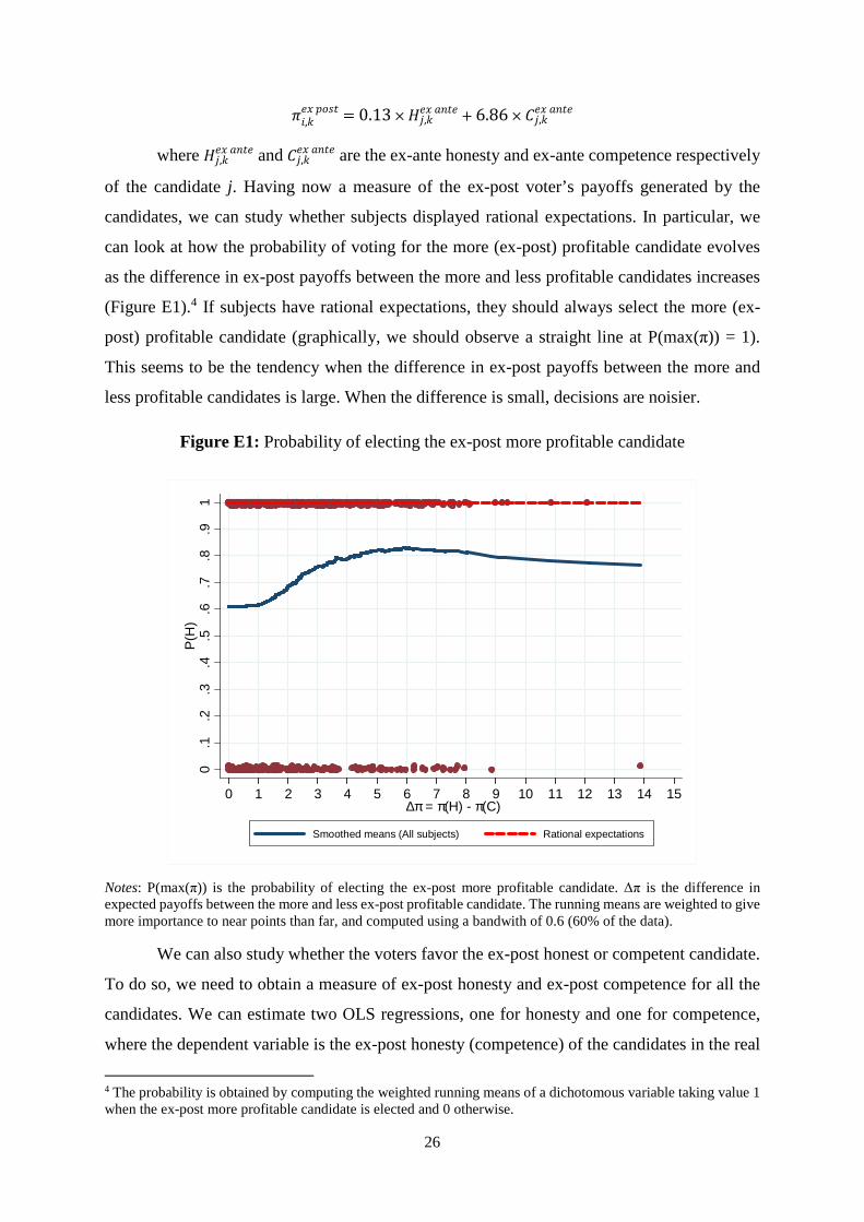
26

��,�������

= 0.13��,��� !��

+ 6.86 × ��,��� !��

where ��,��� !�� and ��,�

�� !�� are the ex-ante honesty and ex-ante competence respectively

of the candidate j. Having now a measure of the ex-post voter’s payoffs generated by the

candidates, we can study whether subjects displayed rational expectations. In particular, we

can look at how the probability of voting for the more (ex-post) profitable candidate evolves

as the difference in ex-post payoffs between the more and less profitable candidates increases

(Figure E1).4 If subjects have rational expectations, they should always select the more (ex-

post) profitable candidate (graphically, we should observe a straight line at P(max(π)) = 1).

This seems to be the tendency when the difference in ex-post payoffs between the more and

less profitable candidates is large. When the difference is small, decisions are noisier.

Figure E1: Probability of electing the ex-post more profitable candidate

Notes: P(max(π)) is the probability of electing the ex-post more profitable candidate. ∆π is the difference in expected payoffs between the more and less ex-post profitable candidate. The running means are weighted to give more importance to near points than far, and computed using a bandwith of 0.6 (60% of the data).

We can also study whether the voters favor the ex-post honest or competent candidate.

To do so, we need to obtain a measure of ex-post honesty and ex-post competence for all the

candidates. We can estimate two OLS regressions, one for honesty and one for competence,

where the dependent variable is the ex-post honesty (competence) of the candidates in the real

4 The probability is obtained by computing the weighted running means of a dichotomous variable taking value 1 when the ex-post more profitable candidate is elected and 0 otherwise.

0.1

.2.3

.4.5

.6.7

.8.9

1P

(H)

0 1 2 3 4 5 6 7 8 9 10 11 12 13 14 15 ∆π = π(H) - π(C)

Smoothed means (All subjects) Rational expectations

27

situation, while the independent variable is the ex-ante honesty (competence) of the candidates

in the real situation. We can then multiply the estimated coefficients with the ex-ante honesty

and the ex-ante competence respectively of all the candidates (both real and fictional) to obtain

a statistical expected measure of the ex-post honesty and ex-post competence respectively.

Table E2 presents the result of these estimations.

Table E2: OLS regressions on ex-post honesty and competence

Ex-post honesty Ex-post competence b se b se

Ex-ante Honesty 0.823*** 0.035 . . Ex-ante Competence . . 1.241*** 0.024

Obs 90 90 Adj. R2 0.862 0.968

Df 1 1 Prob > F 0 0

Notes: OLS regression. The table reports the beta coefficients and the standard errors. Observations are from the candidates in the real situation. * p < 0.1, ** p < 0.05, *** p < 0.01. The coefficients are not normalized.

Focusing on cases where there is a trade-off between ex-post honesty and ex-post

competence, we can look at how the probability of voting for the more ex-post honesty

candidate evolves if the difference in ex-post payoffs ∆π between the more and less honesty

candidates increases (Figure E2). For ∆π < 0 (i.e. the ex-post more honesty candidate is also

the ex-post less profitable), profit-maximizing subjects with rational expectations should vote

for the ex-post less honesty subjects as he or she is associated with higher ex-post payoffs. For

∆π > 0 (i.e. the ex-post more honest candidate is also the ex-post more profitable), profit-

maximizing subjects with rational expectations should vote for the ex-post more honest

subjects as he or she is associated with higher ex-post payoffs. The figure shows that subjects

did not seem to vote for the ex-post more profitable candidate, as rational expectations would

predict, but the candidate who is ex-post more honest. This pattern is similar to the one

observed for adaptive expectations (see main paper), and, perhaps, even more marked.

28

Figure E2: Probability of electing the ex-post more honest candidate

Notes: P(T) is the probability of electing the more ex-post honest candidate. ∆π is the difference in expected payoffs between the more and less ex-post honest candidate. The running means are weighted to give more importance to near points than far, and computed using a bandwith of 0.6 (60% of the data). The data corresponds to cases where there is a trade-off between ex-post honesty and competence.

We can also conduct a regression analysis like the one in the paper but using the ex-

post measures of honesty and competence. The dependent variable is the dummy ‘Vote’. In

regression 1, the independent variables include the log of ex-post honesty and ex-post

competence of the candidate. In regression 2, we also add interaction terms of log(ex-post

honesty) and log(ex-post competence) with a dummy variable |π|>5 which takes value 1 when

the absolute deviation in ex-post expected payoffs between the two candidates is bigger than 5

experimental points. In regression 3, we control as well for the demographic, psychological

and behavioral characteristics of the voters and treatment effects by interacting them with

log(ex-post honesty) and log(ex-post competence).5 Table E3 displays the results of the

regressions.6

5 As we already explained in the paper, since the characteristics of the voters do not vary over the choices of the voters, in the regression we can only have interaction terms between the alternative-specific variables and the voter-specific variables. 6 The full regressions are available upon request.

0.1

.2.3

.4.5

.6.7

.8.9

1P

(T)

-10 -9 -8 -7 -6 -5 -4 -3 -2 -1 0 1 2 3 4 5 6 7 8 9 10 ∆π = π(H) - π(C)

Smoothed means (All subjects) Theoretical prediction

Smoothed means (No inconsistent)

29

Table E3: Alternative-specific conditional logit regressions

Regression 1 Regression 2 Regression 3 b se b se b se

log(Honesty) 5.284*** 0.888 5.424*** 0.949 10.435*** 1.941 log(Competence) 3.037*** 0.5 3.196*** 0.49 4.852*** 1.335

log(Honesty) × |π|>5 -0.669 1.964 -1.35 1.449 log(Competence) × |π|>5 -0.827 1.116 -1.101 0.77

Interactions with demographic, behavioral, psychological and

treatment variables No No Yes

Obs 1334 1334 1334 1334 Pseudo R2 0.212 0.214 0.267 0.212

Df 2 4 28 2 Prob > F 0 0 0 0

Notes: Alternative-specific logit regression with clustered robust standard errors. The table reports the beta coefficients and the standard errors. The demographic variables are age, gender (= 1 for men), economics background (= 1 if applicable), nationality (Not French = 1 for non French subjects), and University status (= 1 for undergraduate students). The behavioral variables are the competence and honesty of the voter in Stage 1, and whether the subject is classified as inconsistent. The psychological variables are the risk attitude, the SDS17 score and MACH score. The treatment variable is the Belief treatment. The psychological and behavioral variables and age are centered at the mean in order to control for high correlation between the independent variables (see Marquardt, 1980). The data correspond to cases where there was a trade-off between ex-post honesty and ex-post competence. The full regressions are available from the authors upon request. * p < 0.1, ** p < 0.05, *** p < 0.01.

In Regressions 1-3, both the coefficients of log(honesty) and log(competence) are

positive and strongly significantly. The coefficient of log(honesty) is also significantly larger

than the coefficient of log(competence) (χ2 tests, p < 0.001). This indicates that, if we assume

that voters have rational expectations, the bias towards caring about honesty carries through. If

we control for the difference in ex-post expected payoffs between the two candidates

(Regressions 2), we find that the bias characterize both small and large differences. Alltogher

these results support the key finding of the paper that people care about the honesty of the

candidates.

Finally, we can compare how many electoral choices were consistent with rational

expectations and how many electoral choices were consistent with adaptive expectations. This

information is summarized in Tables E4 and E5. Both tables show that a significant proportion

of choices were consistent with either adaptive or rational expectations. In addition, they

suggest that more choices display adaptive (84.38% for all the subjects, 88.08% if we exclude

the inconsistent subjects) rather than rational (75.30% for all the subjects, 78.31% if we exclude

the inconsistent subjects) expectations (χ2 test, p < 0.001).

30

Table E4: Electoral choices consistent with adaptive or rational expectations

All subjects No inconsistent subjects Adaptive

expectations No Belief Belief Total No Belief Belief Total

NO 116 (25.78%)

111 (25.34%)

227 (25.56%)

106 (24.65%)

93 (24.6%) 199

(24.63%)

YES 334 (74.22%)

327 (74.66%)

661 (74.44%)

324 (75.35%)

285 (75.4%)

609 (75.37%)

Total 450 (100%)

438 (100%)

888 (100%)

430 (100%)

378 (100%)

808 (100%)

Rational expectations

No Belief Belief Total No Belief Belief Total

NO 125 (27.78%)

130 (29.68%)

255 (28.72%)

115 (26.74%)

109 (28.84%)

224 (27.72%)

YES 325 (72.22%)

308 (70.32%)

633 (71.28%)

315 (73.26%)

269 (71.16%)

584 (72.28%)

Total 450 (100%)

438 (100%)

888 (100%)

430 (100%)

378 (100%)

808 (100%)

Table E5: Electoral choices consistent with adaptive and/or rational expectations

No Belief Rational expectations Adaptive expectations NO YES Total

NO 102 (22.67%) 14 (3.11%) 116 (25.78%) YES 23 (5.11%) 311 (69.11%) 334 (74.22%) Total 125 (27.78%) 325 (72.22%) 450 (100%) Belief Rational expectations

Adaptive expectations NO YES Total NO 101 (23.06%) 10 (2.28%) 111 (25.34%) YES 29 (6.62%) 298 (68.04%) 327 (74.66%) Total 130 (29.68%) 308 (70.32%) 438 (100%)

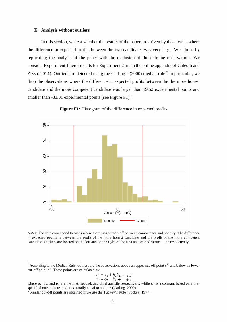
31

E. Analysis without outliers

In this section, we test whether the results of the paper are driven by those cases where

the difference in expected profits between the two candidates was very large. We do so by

replicating the analysis of the paper with the exclusion of the extreme observations. We

consider Experiment 1 here (results for Experiment 2 are in the online appendix of Galeotti and

Zizzo, 2014). Outliers are detected using the Carling’s (2000) median rule.7 In particular, we

drop the observations where the difference in expected profits between the the more honest

candidate and the more competent candidate was larger than 19.52 experimental points and

smaller than -33.01 experimental points (see Figure F1).8

Figure F1: Histogram of the difference in expected profits

Notes: The data correspond to cases where there was a trade-off between competence and honesty. The difference in expected profits is between the profit of the more honest candidate and the profit of the more competent candidate. Outliers are located on the left and on the right of the first and second vertical line respectively.

7 According to the Median Rule, outliers are the observations above an upper cut-off point %& and below an lower cut-off point %'. These points are calculated as:

%& = () + �)((� − (,) %' = () − �)((� − (,)

where (,, (), and (� are the first, second, and third quartile respectively, while �) is a constant based on a pre-specified outside rate, and it is usually equal to about 2 (Carling, 2000). 8 Similar cut-off points are obtained if we use the Tuckey’s Rule (Tuckey, 1977).

0.0

1.0

2.0

3.0

4.0

5

-50 0 50 ∆π = π(H) - π(C)

Density Cutoffs

32

Figure F2 shows the probability of electing the more honest candidate as a function of

the difference in expected payoffs between the more and less honest candidate (as in Figure 2

of the paper). Even once we exclude the extreme cases, the area below the weighted running

means for ∆π < 0 is bigger than the area above the weighted running means for ∆π > 0. We

also replicate the regression analysis of the paper (Table F1). With the removal of the outliers,

the results do not change. In particular, the coefficient of log(honesty) is significantly larger

than the coefficient of log(competence) in all the regressions (χ2 tests, p < 0.05).

Figure F2: Probability of electing the more honest candidate

Notes: P(T) is the probability of electing the more honest candidate. ∆π is the difference in expected payoffs between the more and less honest candidate. The running means are weighted to give more importance to near points than far, and computed using a bandwith of 0.6 (60% of the data).

0.1

.2.3

.4.5

.6.7

.8.9

1P

(H)

-35 -30 -25 -20 -15 -10 -5 0 5 10 15 20 25 ∆π = π(H) - π(C)

No Belief treatment

0.1

.2.3

.4.5

.6.7

.8.9

1P

(H)

-35 -30 -25 -20 -15 -10 -5 0 5 10 15 20 25 ∆π = π(H) - π(C)

(based on actual information)Belief treatment

0.1

.2.3

.4.5

.6.7

.8.9

1P

(H)

-35 -30 -25 -20 -15 -10 -5 0 5 10 15 20 25 ∆π = π(H) - π(C)

(based on beliefs)Belief treatment

0.1

.2.3

.4.5

.6.7

.8.9

1P

(H)

-35 -30 -25 -20 -15 -10 -5 0 5 10 15 20 25 ∆π = π(H) - π(C)

(based on actual information)All treatments

Smoothed means (All subjects) Theoretical prediction

Smoothed means (No inconsistent)

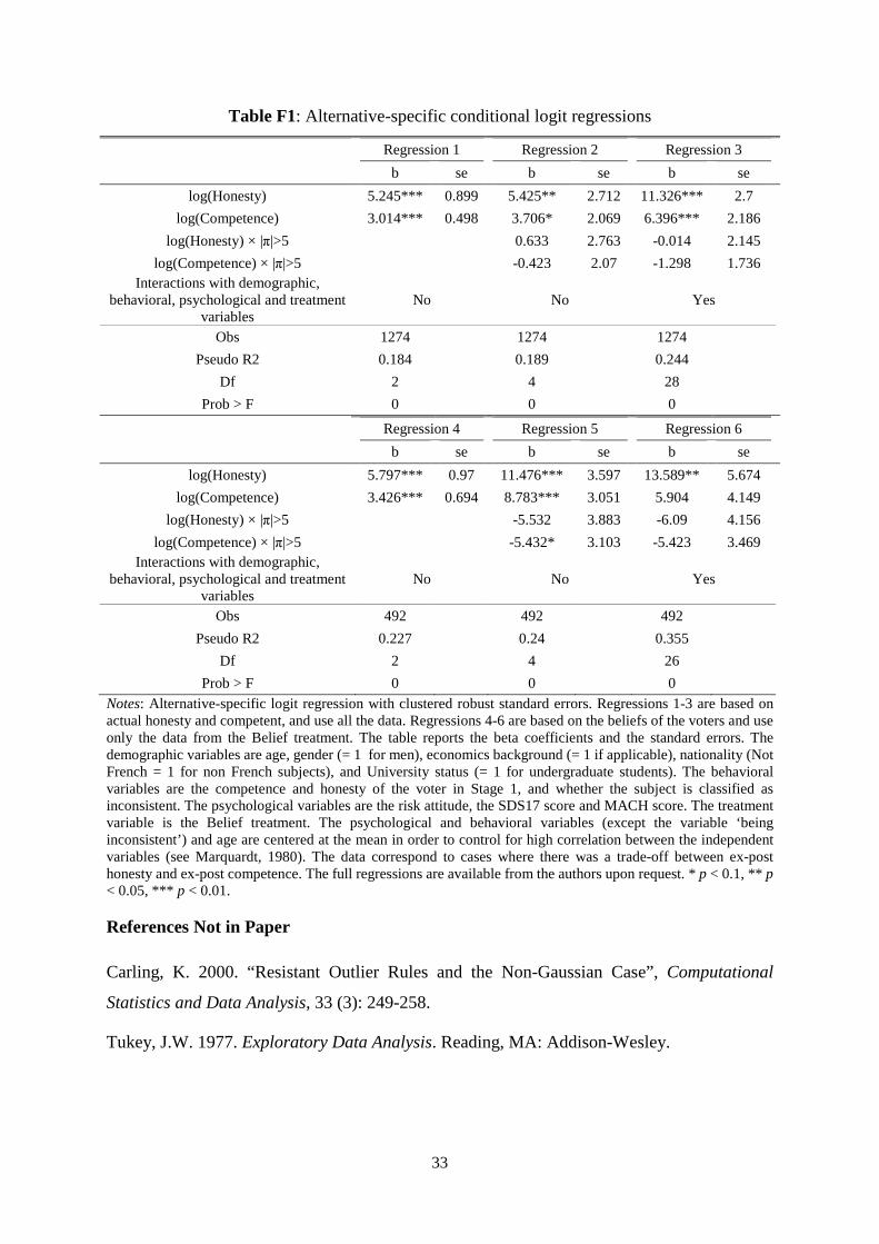
33

Table F1: Alternative-specific conditional logit regressions

Regression 1 Regression 2 Regression 3

b se b se b se

log(Honesty) 5.245*** 0.899 5.425** 2.712 11.326*** 2.7

log(Competence) 3.014*** 0.498 3.706* 2.069 6.396*** 2.186

log(Honesty) × |π|>5 0.633 2.763 -0.014 2.145

log(Competence) × |π|>5 -0.423 2.07 -1.298 1.736 Interactions with demographic,

behavioral, psychological and treatment variables

No No Yes

Obs 1274 1274 1274

Pseudo R2 0.184 0.189 0.244

Df 2 4 28

Prob > F 0 0 0

Regression 4 Regression 5 Regression 6

b se b se b se

log(Honesty) 5.797*** 0.97 11.476*** 3.597 13.589** 5.674

log(Competence) 3.426*** 0.694 8.783*** 3.051 5.904 4.149

log(Honesty) × |π|>5 -5.532 3.883 -6.09 4.156

log(Competence) × |π|>5 -5.432* 3.103 -5.423 3.469 Interactions with demographic,

behavioral, psychological and treatment variables

No No Yes

Obs 492 492 492

Pseudo R2 0.227 0.24 0.355

Df 2 4 26

Prob > F 0 0 0 Notes: Alternative-specific logit regression with clustered robust standard errors. Regressions 1-3 are based on actual honesty and competent, and use all the data. Regressions 4-6 are based on the beliefs of the voters and use only the data from the Belief treatment. The table reports the beta coefficients and the standard errors. The demographic variables are age, gender (= 1 for men), economics background (= 1 if applicable), nationality (Not French = 1 for non French subjects), and University status (= 1 for undergraduate students). The behavioral variables are the competence and honesty of the voter in Stage 1, and whether the subject is classified as inconsistent. The psychological variables are the risk attitude, the SDS17 score and MACH score. The treatment variable is the Belief treatment. The psychological and behavioral variables (except the variable ‘being inconsistent’) and age are centered at the mean in order to control for high correlation between the independent variables (see Marquardt, 1980). The data correspond to cases where there was a trade-off between ex-post honesty and ex-post competence. The full regressions are available from the authors upon request. * p < 0.1, ** p < 0.05, *** p < 0.01. References Not in Paper

Carling, K. 2000. “Resistant Outlier Rules and the Non-Gaussian Case”, Computational

Statistics and Data Analysis, 33 (3): 249-258.

Tukey, J.W. 1977. Exploratory Data Analysis. Reading, MA: Addison-Wesley.