Embed Size (px)
Citation preview
COMPENDIUM ON GREENHOUSE GAS BASELINES AND MONITORINGPASSENGER AND FREIGHT TRANSPORT
Handbook on
MEASUREMENT, REPORTING AND VERIFICATIONFOR DEVELOPING COUNTRY PARTIES
On behalf of:
of the Federal Republic of Germany Empowered lives. Resilient nations.


COMPENDIUM ON GREENHOUSE GAS BASELINES AND MONITORINGPASSENGER AND FREIGHT TRANSPORT

Compendium on GHG Baselines and MonitoringPassenger and freight transport
4
Coordinating lead authors:
Urda Eichhorst (GIZ)
Daniel Bongardt (GIZ)
Victoria Novikova (UNFCCC)
Lead authors:
Charles Kooshian (CCAP)
Contributing authors:
Francisco Posada (ICCT)
Zifei Yang (ICCT)
Kate Blumberg (ICCT)
Steve Winkelman (CCAP)
Expert reviewers:
Bert Fabian (UNEP)
Jürg Füssler (Infras)
Andrea Henkel (GIZ)
Cornie Huizinga (SLoCaT)
Alan McKinnon (Kühne Logistics University)
Marion Vieweg-Mersmann (Current Future)
Amr Osama Abdel-Aziz (INTEGRAL Consult)
Francisco Posada Sanchez (ICCT)
Ernst-Benedikt Riehle (GIZ)
Alexandra Soezer (UNDP)
James Vener (UNDP)
Noak Westerberg (Swedish EA)
Disclamer: The views expressed herein are those of the authors and do not necessarily reflect the views of the organizations
they represent, in particular, the United Nations and UNFCCC and GIZ. This is the first edition of the Passenger and Freight
Transport Volume. The volume will be updated once more in the second half of 2017, adding Chapter 8 on Pricing Policies, the
methodology for which is currently under development by the Initiative for Climate Action Transparency (ICAT). If you have
any feedback to the current volume or would like to add additional methodologies, please do not hesitate to contact

Compendium on GHG Baselines and MonitoringPassenger and freight transport
5
TABLE OF CONTENTS
1 GLOSSARY
1 ABBREVIATIONS
1 INTRODUCTION
4 OVERVIEW OF THE SECTOR
Approaches to estimating transport emissions
Top-down approach
Bottom-up approach
The ASIF model
Life cycle emissions
Leakage
Rebound effects
Determining the baseline and calculating emissions
Purpose of analysis
Baseline setting
Approaches to determining the emissions reduction
4 READER GUIDE TO THE MITIGATION ACTION SECTIONS OF THE TRANSPORT VOLUME
Description and characteristics of action type
Structure of mitigation effects
Determining the baseline and calculating emission reductions
Guidance on the selection of analysis tools for the mitigation action type
Monitoring
Example
1 CHAPTER 1: MASS TRANSIT INVESTMENTS
1.1. Description and characteristics of mass transit investments
1.2. Structure of mitigation effects
1.3. Determining the baseline and calculating emission reductions
1.4. Guidance on the selection of analysis tools for mass transit investments
1.5. Monitoring
1.6. Example – Colombia Transmilenio
2 CHAPTER 2: COMPREHENSIVE URBAN TRANSPORT PROGRAMMES AND PLANS
2.1. Description and characteristics of urban transport programmes and plans
2.2. Structure of mitigation effects
2.3. Determining the baseline and calculating emission reductions
2.4. Guidance on the selection of analysis tools for comprehensive urban mobility programmes or plans
2.5. Monitoring
2.6. Example – Jakarta travel demand management
3 CHAPTER 3: VEHICLE EFFICIENCY IMPROVEMENT PROGRAMMES
3.1. Description and characteristics of vehicle efficiency improvement programmes
3.2. Structure of mitigation effects
3.3. Determining the baseline and calculating emission reductions
9
12
13
15
16
16
18
18
18
19
19
19
20
21
24
24
25
25
25
25
29
29
32
34
40
40
43
43
47
48
54
54
57
57
60

Compendium on GHG Baselines and MonitoringPassenger and freight transport
6
3.4. Guidance on the selection of analysis tools for vehicle efficiency improvement programmes
3.5. Monitoring
3.6. Example – Mexican freight NAMA
4 CHAPTER 4: ALTERNATIVE FUELS INCENTIVES, REGULATION AND PRODUCTION
4.1. Description and characteristics of alternative fuels incentives, regulation and production mitigation actions
4.2. Structure of mitigation effects
4.3. Determining the baseline and calculating emission reductions
4.4. Guidance on the selection of analysis tools for alternative fuels mitigation actions
4.5. Monitoring
4.6. Example – Paraguay plant oil production
5 CHAPTER 5: INTER-URBAN RAIL INFRASTRUCTURE
5.1. Description and characteristics of inter-urban rail investments
5.2. Structure of mitigation effects
5.3. Determining the baseline and calculating emission reductions
5.4. Guidance on the selection of analysis tools for inter-urban rail infrastructure mitigation actions
5.5. Monitoring
5.6. Example – India railway NAMA
6 CHAPTER 6: SHIFT MODE OF FREIGHT TRANSPORT FROM ROAD TO RAIL OR WATER
6.1. Description and characteristics of freight modal shift mitigation actions
6.2. Structure of mitigation effects
6.3. Determining the baseline and calculating emission reductions
6.4. Guidance on the selection of analysis tools for freight modal shift projects
6.5. Monitoring
6.6. Example – Switching freight to short sea shipping (Brazil)
7 CHAPTER 7: NATIONAL FUEL ECONOMY STANDARD
7.1. Description and characteristics of GHG/FE standards for light-duty vehicles
7.2. Structure of mitigation effects
7.3. Determining the baseline and calculating emission reductions
7.4. Guidance on the selection of analysis tools for new vehicle GHG and fuel economy standards for light-duty vehicles
7.5. Monitoring
7.6. Example – Impact of new vehicle CO2 standards in Mexico
8 CHAPTER 8: PRICING POLICIES
BIBLIOGRAPHY
63
68
69
71
71
74
76
78
79
81
81
85
86
90
90
93
93
97
98
102
103
105
106
112
115
119
120
122
123

Compendium on GHG Baselines and MonitoringPassenger and freight transport
7
Figures
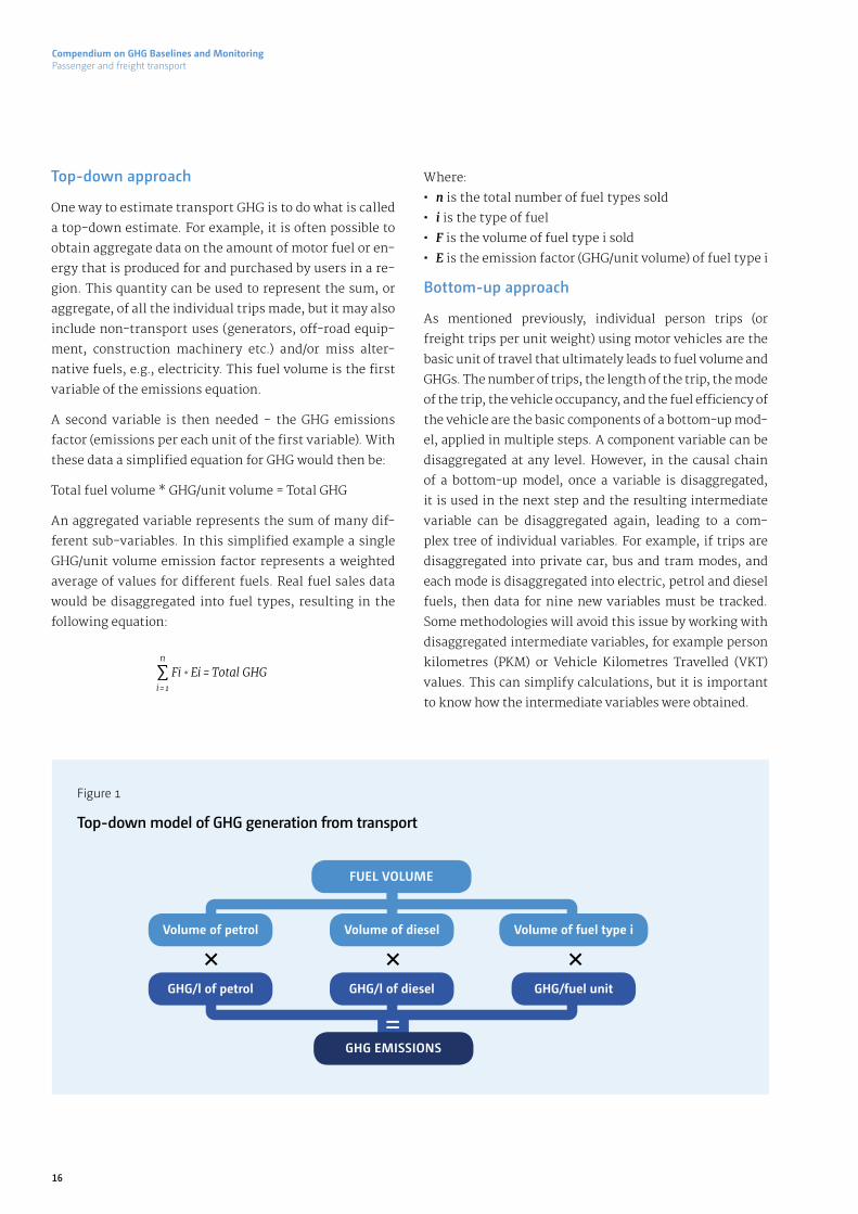
Figure 1 Top-down model of GHG generation from transport
Figure 2 Bottom-up mode of GHG generation from transport
Figure 3 Mapping life cycle GHG emissions in the transport sector
Figure 4 Mitigation outcome of an action
Figure 5 Guide to causal chain graphics
Figure 6 Navigating classes of available methods and associated tools
Figure 7 Mass transit investments Causal Chain
Figure 8 Navigating classes of available methods and associated tools for mass transit investment mitigation actions
Figure 9 Comprehensive urban transport programmes and plans Causal Chain
Figure 10 Navigating classes of available methods and associated tools for comprehensive urban transport programmes and plans
Figure 11 Vehicle fuel efficiency improvement programmes Causal Chain
Figure 12 Causal Chain of emissions from RAC
Figure 13 Navigating classes of available methods and associated tools for vehicle fuel efficiency improvement programmes
Figure 14 Alternative fuels incentives Causal Chain
Figure 15 Navigating classes of available methods and associated tools for alternative fuels mitigation actions
Figure 16 Inter-urban rail infrastructure (passenger) mitigation actions Causal Chain
Figure 17 Inter-urban rail infrastructure (freight) mitigation actions Causal Chain
Figure 18 Navigating classes of available methods and associated tools for inter urban rail mitigation actions
Figure 19 Freight modal shift
Figure 20 Navigating classes of available methods and associated tools of freight modal shift mitigation actions
Figure 21 Passenger car sales CO2 emission targets and sales weighted averaged actual fleet historical performance
Figure 22 Causal chain for new vehicle fuel economy and greenhouse gas emission standards
Figure 23 Historic progression of passenger car fleet average CO2 emission standards and fleet performance
Figure 24 Navigating classes of available methods and associated tools for new vehicle fuel economy standards
Tables
Table 1 Characteristics of mitigation actions
Table 2 Dimensions of boundary setting for mass transit investment mitigation actions
Table 3 Actions with potential for double counting for mass transit investment mitigation actions
Table 4 Level of disaggregation of key variables for mass transit investment mitigation actions
Table 5 Travel demand models for mass transit investment mitigation actions
16
17
19
21
25
27
30
35
44
50
58
62
64
72
76
82
83
87
94
99
105
107
113
117
14
31
32
34
36

Compendium on GHG Baselines and MonitoringPassenger and freight transport
8
Table 6 Disaggregated bottom-up ex-post guidance for mass transit investment mitigation actions
Table 7 Partially aggregated bottom-up spreadsheet tools with defaults for mass transit investment mitigation actions
Table 8 Simple bottom-up tools with mostly default data for mass transit investment mitigation actions
Table 9 Historical trends or expert judgment tools for mass transit investment mitigation actions
Table 10 Minimum indicator set for mass transit mitigation action
Table 11 Dimensions of boundary setting for comprehensive urban transport programmes and plans
Table 12 Actions with potential for double counting for comprehensive urban transport programmes and plans
Table 13 Level of disaggregation of key variables for comprehensive urban transport programmes and plans
Table 14 Travel demand models for comprehensive urban transport programmes and plans
Table 15 Disaggregated bottom-up ex-post guidance for comprehensive urban transport programmes and plans
Table 16 Partially aggregated bottom-up spreadsheet tools with defaults for comprehensive urban transport programmes and plans
Table 17 Simple bottom-up tools with mostly default data for comprehensive urban transport programmes and plans
Table 18 Minimum indicator set for comprehensive urban transport programme or plan mitigation actions (passenger transport)
Table 19 Dimensions of boundary setting for vehicle fuel efficiency improvement programmes
Table 20 Actions with potential for double counting for vehicle fuel efficiency improvement programmes
Table 21 Additional variables for higher accuracy for vehicle fuel efficiency improvement programmes
Table 22 Disaggregate emissions models for vehicle fuel efficiency improvement programmes
Table 23 Disaggregated bottom-up ex-post guidance for vehicle fuel efficiency improvement programmes
Table 24 Simple bottom-up tools with mostly default data for vehicle fuel efficiency improvement programmes
Table 25 Minimum indicator set for vehicle fuel efficiency improvement programmes
Table 26 Dimensions of boundary setting for alternative fuels mitigation actions
Table 27 Actions with potential for double counting for alternative fuels mitigation actions
Table 28 Level of disaggregation of key variables for alternative fuels mitigation actions
Table 29 Disaggregate emissions models for alternative fuels mitigation actions
Table 30 Disaggregated bottom-up ex-post guidance for alternative fuels mitigation actions
Table 31 Simple bottom-up tools with mostly default data for alternative fuels mitigation actions
Table 32 Minimum indicator set for alternative fuel mitigation action
Table 33 Dimensions of boundary setting for inter urban rail mitigation actions
Table 34 Actions with potential for double counting for inter urban rail mitigation actions
Table 35 Level of disaggregation of key variables for inter urban rail mitigation actions
Table 36 Travel demand models for inter urban rail mitigation actions
37
38
39
39
40
46
47
49
51
52
53
54
55
59
59
63
65
66
68
68
73
74
75
77
78
79
79
84
85
86
88

Compendium on GHG Baselines and MonitoringPassenger and freight transport
9
Table 37 Disaggregated bottom-up ex-post guidance for inter urban rail mitigation actions
Table 38 Partially aggregated bottom-up spreadsheet tools with defaults for inter urban rail mitigation actions
Table 39 Simple bottom-up tools with mostly default data for inter urban rail mitigation actions
Table 40 Minimum indicator set for Inter urban rail mitigation action
Table 41 Dimensions of boundary setting of freight modal shift mitigation actions
Table 42 Actions with potential for double counting of freight modal shift mitigation actions
Table 43 Level of disaggregation of key variables of freight modal shift mitigation actions
Table 44 Travel demand models for freight modal shift mitigation actions
Table 45 Disaggregated bottom-up ex-post guidance for freight modal shift mitigation actions
Table 46 Partially aggregated bottom-up spreadsheet tools with defaults for freight modal shift mitigation actions
Table 47 Simple bottom-up tools with mostly default data for freight modal shift mitigation actions
Table 48 Minimum indicator set for freight mode shift mitigation actions
Table 49 Factors that affect key GHG/FE standards variables
Table 50 Dimensions of boundary setting for new-vehicle GHG/FE standards
Table 51 Main GHG/FE modeling uncertainties
Table 52 Level of disaggregation of key variables
Table 53 GHG/ FE Inventory models
Table 54 Minimum indicator set for new vehicle GHG/FE standards mitigation actions
Boxes
Box 1 Example of variation in trips
Box 2 Reference document on measurement, reporting and verification in the transport sector
Box 3 MRV of mobile air conditioning and transport refrigeration mitigation actions
Box 4 Vehicle energy measurement units
89
89
90
91
95
96
98
100
101
101
102
103
109
110
115
116
118
119
15
20
61
106
GLOSSARY
Activity data
Additionality
Base year
A quantitative measure of a level of economic activity that results in GHG emissions. Activity data
is multiplied by an emission factor to estimate the GHG emissions associated with a process or
an operation.
A criterion of CDM that asks if the projects or programme might occur without the financial input
from emission credits.
A specific year of historical data against which emissions are compared over time.

Compendium on GHG Baselines and MonitoringPassenger and freight transport
10
Baseline scenario
Baseline scenario
assumption
Business- as-usual (BAU)
scenario
CO2 equivalent (CO2e)
Cumulative emissions
Double counting
Dynamic baseline scenario
Emissions driver
Emission factor
Emission reduction
Ex-ante
Ex-post
Greenhouse gas (GHG)
Inventory
Leakage
Mitigation action
Mitigation scenario
Mode
Model
Baseline scenarios are projections of GHG emissions and their key drivers as they might evolve in
a future in which no explicit actions are taken to reduce GHG emissions.
A quantitative value that defines how an emissions driver in a baseline scenario is most likely to
change over a defined future time period.
A reference case that represents future events or conditions most likely to occur as a result of
implemented and adopted policies and actions.
Sometimes used as an alternative term instead of “baseline scenario”. (See Volume 1)
The universal unit of measurement to indicate the global warming potential (GWP) of each
greenhouse gas, expressed in terms of the GWP of 1 unit of carbon dioxide. It is used to evaluate
releasing (or avoiding releasing) different greenhouse gases against a common basis.
Sum of annual emissions over a defined time period.
Occurs when the same transferable emissions unit is counted toward the mitigation goal of more
than one jurisdiction or action. Double counting includes double claiming, double selling, and
double issuance of units.
Baseline scenario that is recalculated based on changes in emissions drivers.
Socioeconomic or other conditions or other policies/actions that influence the level of emissions
or removals. For example, economic growth is a driver of increased energy consumption. Drivers
that affect emissions activities are divided into two types: policies or actions and non-policy
drivers.
A carbon intensity factor that converts activity data into GHG emissions data, usually given in
gram carbon dioxide equivalents per kilometre (gCO2eq/km).
Reduction in greenhouse emissions relative to a base year or baseline scenario
Analysis that is done before an intervention is taken
Analysis that is done after an intervention is taken
Gases that trap heat in the atmosphere, including Carbon dioxide (CO2), Methane (CH4), Nitrous
oxide (N2O), and Fluorinated gases.
An analysis of the quantity of emissions that occurred over a given period of time in the past,
broken down by sources.
Increase in emissions outside of the boundary of a mitigation action that result as a consequence
of mitigation actions, such as policies, actions, and projects, implemented to meet the goal.
A policy, programme, project or measure that is expected to reduce GHG emissions if it is
implemented. A mitigation action is an intervention.
A mitigation scenario presents future emissions with the assumption of the introduction of
certain policies and measures targeting GHG emissions reductions.
The method of travel, usually the type of transport system that is used.
A framework used to represent the operation and/or the characteristics and/or the reactions of a
more complex (natural, engineering or socioeconomic) process.

Compendium on GHG Baselines and MonitoringPassenger and freight transport
11
Transport modes that require no energy source other than human effort. Usually walking or
human powered vehicles.
A variable that is part of an equation (here) used to estimate emissions. For example, “emissions
per litre of petrol” and “litres of petrol” are both parameters in the equation “2.34 kg CO2e/l of
petrol × 100 litres = 234 kg CO2e.”
Distance travelled by a person or passenger multiplied by the number of persons or passengers.
A set of formally described, adopted or planned legal actions, rules, guidelines to be followed and/
or enforced by a government or authority. A policy typically includes its area and date of validity,
its implementing organisations, and its objectives.
An estimation of the evolution of certain parameters, indicators, variables (e.g., fuel cost,
population, etc.) based on a set of assumptions and optionally a model (depending on the
approach chosen).
A year against which commitments are made and measured, typically in the form of emission
abatement. Most frequently it is a year in the past, for example 1990 for the Annex I Parties
commitments under the Kyoto Protocol, but in some cases it is a future year. Occasionally it can
be set as an average of a period of years (as is the case of the base year for some countries with
economies in transition under the Kyoto Protocol).
The description of several key variables in a possible state of the future. Scenarios are used when
the total number of possible combinations of variable states is too great to analyse efficiently.
A scenario has to be plausible in the sense that under certain assumptions it can occur and
should contain consistent and coherent outcomes. A scenario is not a probabilistic forecast but a
deterministic description of a situation whose actual probability is not completely known.
A method to understand differences resulting from changes in methodological choices and
assumptions and to explore model sensitivities to inputs. The method involves varying the
parameters to understand the sensitivity of the overall results to changes in those parameters.
Static baselines use a given year or the average of several years as a reference value. A static
baseline can also be defined as a reference level using an estimation which is not based on a
reference year or the average of years, but which remains fixed throughout all monitoring years
and is not recalculated
Mixed use residential and commercial urban development centred around access to public transport.
A general term that refers to the lack of certainty in data and methodology choices, such as the
application of non- representative factors or methods, incomplete data on sources and sinks, or
lack of transparency. It can also be measurement that characterizes the dispersion of values that
could reasonably be attributed to a parameter.
Distance travelled by a vehicle multiplied by number of vehicles
Distance travelled by a tonne of freight multiplied by number of tonnes
Non-motorized transport
(NMT)
Parameter
Person kilometres (or
passenger kilometres) (PKM)
Policy
Projection
Reference year
Scenario
Sensitivity analysis
Static baseline
Transit Oriented
Development (TOD)
Uncertainty
Vehicle kilometres travelled
(VKT)
Tonne kilometres (TKM)

Compendium on GHG Baselines and MonitoringPassenger and freight transport
12
ABBREVIATIONS
ASIF
BAU
BRT
CDM
FE
GIZ
GHG
MRV
MYC
NAMA
NMT
OECD
PKM
SLoCaT
SUMP
TKM
TOD
UNFCCC
VKT
Activity, Share, Intensity, Fuel
Business as usual
Bus Rapid Transit
Clean Development Mechanism
Fuel economy
Deutsche Gesellschaft für Internationale Zusammenarbeit GmbH
Greenhouse gas
Measurement, Reporting and Verification
MobiliseYourCity
Nationally Appropriate Mitigation Action
Non-motorized transport
Organisation for Economic Co-operation and Development
Person kilometres (or passenger kilometres)
Partnership for Sustainable Low-carbon Transport
Sustainable Urban Mobility Plan
Tonne kilometres
Transit Oriented Development
United Nations Framework Convention on Climate Change
Vehicle kilometres travelled

Compendium on GHG Baselines and MonitoringPassenger and freight transport
13
Transport related emissions are growing worldwide.
Transport currently accounts for about 28% of total end-
use energy. Greenhouse gas (GHG) emissions from the
transport sector have more than doubled since 1970, and
have increased at a faster rate than any other energy end-
use sector to reach 7.0 Gt CO2 eq in 2010. The IPCC has
found that without mitigation actions, transport emis-
sions could increase at a faster rate than emissions from
the other energy end-use sectors and reach around 12 Gt
CO2eq/yr by 2050 (IPPC, 2014).
Much of this growth will come from transport demand
per capita in developing and emerging economies, which
is expected to increase at a much faster rate in the next
decades due to rising incomes and development of infra-
structure. Two thirds of the growth in light duty vehicle
ownership, which is expected to double in the next few
decades, will be in non-OECD countries. In OECD coun-
tries VKT per capita has tended to stabilize, but freight and
air passenger transport has continued to increase. Also for
freight transport, economic globalization has increased
the volume and distance of movement of goods and ma-
terials worldwide. If no additional measures are taken,
CO2 emissions from global freight alone could increase by
160%, as international freight volumes grow threefold by
2050, largely due to increased use of road transport, espe-
cially for short distances and in regions that lack rail links,
such as South-East Asia (OECD/ITF, 2017).
However, decoupling of transport GHG emissions from
economic growth may be possible. GHG emissions from
passenger and freight transport can be reduced by a range
of both technological and behavioral mitigation actions.
Since rebound effects can reduce the CO2 benefits of purely
technological efficiency improvements, a balanced pack-
age of actions has the best chance of achieving maximum
mitigation effects. Broadly, mitigation actions fall into
three categories:
· Avoiding journeys where possible — achieved by actions
such as changing urban form, improving freight logis-
tics systems, substituting information and communica-
tion technologies (ICT) for travel, etc.;
· Modal shift to lower-carbon transport systems —
achieved mainly by increasing investment in public
transport, walking and cycling infrastructure;
· Improving the energy intensity of travel per passen-
ger km or tonne km — by improving vehicle and engine
performance, or overall transport system performance;
· Reducing carbon intensity of fuels by replacing oil
based fossil fuels with natural gas, bio-methane, or
biofuels, or electricity or hydrogen produced from re-
newable energy sources.
INTRODUCTION

Compendium on GHG Baselines and MonitoringPassenger and freight transport
14
Scale ASIF lever Mode
• Project level• City-regional level• National
• Travel activity
• Mode shift
• Energy intensity
• Fuel type
• Non-motorized
• Transit/ bus/ trolley/etc.
• Private vehicle
• Freight
The development of effective transport climate strate-
gies to implement appropriate and cost effective mitiga-
tion actions rests upon the availability of comprehensive
data and the application of sound assessment methods
for emission reduction potentials. Unfortunately, many
countries lack comprehensive transport emission inven-
tories and mitigation scenario analysis to inform sound
climate action planning. One effort to build capacity in
this area is the development of a Compendium on GHG
Baselines and Monitoring (hereinafter referred to as the
compendium).
The passenger and freight transport volume was coor-
dinated by the Deutsche Gesellschaft für Internationale
Zusammenarbeit (GIZ) in cooperation with the UNFCCC
Secretariat with funding from the German Federal Min-
istry for the Environment, Nature Conservation, Building
and Nuclear Safety (BMUB) and written with the assis-
tance of the Center for Clean Air Policy (CCAP).
The methodologies presented in the Transport Volume
were chosen with a view to cover a broad range of dif-
ferent mitigation action types in terms of scale, type of
intervention and affected modes. In addition, focus was
put on interventions with significant mitigation poten-
tial. The selection was based on SLoCaT’s review of trans-
port methodologies and tools1 and categorised by type of
mitigation action.
The mitigation actions are loosely grouped based on their
geographic scale, mechanism within an ASIF model, and
the affected modes as outlined below.
The remainder of this volume starts with an overview of ap-
proaches on GHG quantification in the transportation sector,
followed by a reader guide to the mitigation action sections.
The main content are eight mitigation action chapters:
· Chapter 1: Mass transit investments: This chapter co-
vers regional or local projects and programs of invest-
ment aimed at shifting travel to public transit modes.
· Chapter 2: Comprehensive urban transport pro-
grammes and plans: This chapter covers regional or
local programmes of planning/investment/policy to
reduce motorized VKT (activity or mode change).
· Chapter 3: Vehicle efficiency improvement pro-
grammes: This chapter covers national/regional level
economic/regulatory tools to affect intensity/fuel type
of passenger transport and freight modes.
· Chapter 4: Alternative fuels incentives, regulation
and production: This chapter covers national or regio-
nal economic or regulatory policies to affect fuel type
for road transport modes.
· Chapter 5: Inter-urban rail infrastructure: This chap-
ter covers national or regional investments aimed at
mode shifting passenger and/or freight trips to rail.
· Chapter 6: Shift mode of freight transport from road
to rail or water: This chapter covers national or regio-
nal investment projects or programmes to shift freight
movement from truck to rail/water.
· Chapter 7: National fuel economy standard: This
chapter covers national regulations to reduce carbon
intensity of passenger and/or freight vehicles.
· Chapter 8: Pricing policies: This chapter covers natio-
nal, regional or local, economic/regulatory/fiscal policy
affecting cost to change activity, mode, and carbon in-
tensity of road transport.
1 <http://slocat.net/sites/default/files/u10/transport_ghg_methodologies_and_tools_-_2017-05-05.xlsx>
Table 1
Characteristics of mitigation actions

Compendium on GHG Baselines and MonitoringPassenger and freight transport
15
APPROACHES TO ESTIMATING TRANSPORT EMISSIONS
Each human decision that causes a person or piece of
freight to travel from an origin to a destination creates
a trip. While many trips are made by walking or other
non-motorized means, millions of trips are made every
day using vehicles powered by combusting hydrocarbons.
Each of these trips produces an amount of GHG emissions,
depending upon the type of vehicle and other characteris-
tics of the trip and energy source or fuel type used.
It is not practical to collect data on the specific charac-
teristics of every trip made every day, in order to add up
the GHG emissions produced. Instead, there are different
methods to simplify to be able to estimate actual or future
emissions:
· Top-down approach
· Bottom-up approach
The following sections will provide the general approach
for both methods, irrespective of the individual mitiga-
tion action.
Box 1
Example of variation in trips
A person in Delhi who rides a motorcycle with a 50cc engine for five kilometres traveling an average of 30 km/hr might
produce 280 grams of CO2e for that trip. Another person, in Dallas, who drives 20 miles in a pickup truck with a 6.4 litre
engine going 120 km/hr might produce 7,800 grams of CO2e during that trip. The next day the person in Delhi could make
the same trip, but he races another motorcycle for two minutes then stops to contemplate an advertisement for new cars
while revving the engine. That same day the Dallas truck driver makes the same trip but she patronizes a drive-through coffee
shop, and then gets stuck in traffic congestion. In both cases the GHG emissions for that person’s second trip will be different.
Finally, imagine that the Dallas pickup truck driver takes three passengers on the same route. The emissions for the vehicle
trip could be still be 7,800 grams but the emissions for each person trip will be 1,950 grams. This suggests that actions for
reducing the emissions of an individual’s trip can be targeted at different levels.
OVERVIEW OF THE SECTOR
Compendium on GHG Baselines and MonitoringPassenger and freight transport
16
Top-down approach
One way to estimate transport GHG is to do what is called
a top-down estimate. For example, it is often possible to
obtain aggregate data on the amount of motor fuel or en-
ergy that is produced for and purchased by users in a re-
gion. This quantity can be used to represent the sum, or
aggregate, of all the individual trips made, but it may also
include non-transport uses (generators, off-road equip-
ment, construction machinery etc.) and/or miss alter-
native fuels, e.g., electricity. This fuel volume is the first
variable of the emissions equation.
A second variable is then needed - the GHG emissions
factor (emissions per each unit of the first variable). With
these data a simplified equation for GHG would then be:
Total fuel volume * GHG/unit volume = Total GHG
An aggregated variable represents the sum of many dif-
ferent sub-variables. In this simplified example a single
GHG/unit volume emission factor represents a weighted
average of values for different fuels. Real fuel sales data
would be disaggregated into fuel types, resulting in the
following equation:
Where:
· n is the total number of fuel types sold
· i is the type of fuel
· F is the volume of fuel type i sold
· E is the emission factor (GHG/unit volume) of fuel type i
Bottom-up approach
As mentioned previously, individual person trips (or
freight trips per unit weight) using motor vehicles are the
basic unit of travel that ultimately leads to fuel volume and
GHGs. The number of trips, the length of the trip, the mode
of the trip, the vehicle occupancy, and the fuel efficiency of
the vehicle are the basic components of a bottom-up mod-
el, applied in multiple steps. A component variable can be
disaggregated at any level. However, in the causal chain
of a bottom-up model, once a variable is disaggregated,
it is used in the next step and the resulting intermediate
variable can be disaggregated again, leading to a com-
plex tree of individual variables. For example, if trips are
disaggregated into private car, bus and tram modes, and
each mode is disaggregated into electric, petrol and diesel
fuels, then data for nine new variables must be tracked.
Some methodologies will avoid this issue by working with
disaggregated intermediate variables, for example person
kilometres (PKM) or Vehicle Kilometres Travelled (VKT)
values. This can simplify calculations, but it is important
to know how the intermediate variables were obtained.
Fi * Ei = Total GHG∑i=1
n
Figure 1
Top-down model of GHG generation from transport
Volume of petrol
GHG/l of petrol
Volume of diesel
GHG/l of diesel
Volume of fuel type i
GHG/fuel unit
FUEL VOLUME
×× ×
=GHG EMISSIONS

Compendium on GHG Baselines and MonitoringPassenger and freight transport
17
Because every trip is a human decision, the intermediate
steps through which a trip results in GHG emissions may
vary. This primarily occurs in the choice of destination
and choice of mode2. Sophisticated travel demand models,
discussed later, attempt to sort out these possibilities in
the trip making process. For purposes of this document,
a typical model of trip making, shown in Figure 2, will be
considered. The figure shows a schematic representation
of a bottom-up model in which persons generate trips,
trips generate PKM leading to vehicle kilometres travelled
(VKT) and finally to fuel consumed. The model for freight
is slightly different, and discussed in Figure 19.
2 For example a person may decide to ride a bicycle to get a cup of coffee before deciding which coffee shop to patronize. Someone with a choice of car, non-motorized transport (NMT) and public transport may choose a coffee shop based on preference for its.
Figure 2
Bottom-up model of GHG generation from transport
DEM
AN
DSU
PPLY
Trips
Vehicles
Emission factors
Fuel
Impr
ove
Shift
Avo
id
PKM
Load factor/Occupancy
Number of veh./Type
Persons
Trips/Person
Km/Trip
Trips/Mode
Km/Vehicle typeVKT
Fuel use
Fuel/Km
GHG/fuel
Upstream GHG/fuel
GHG emissions
Historic and/or default values Intermediate resultsParameters to be monitored
Not considered or only for validation

Compendium on GHG Baselines and MonitoringPassenger and freight transport
18
The ASIF model
This bottom-up model, which as its final step again includes
converting the quantity of fuel consumed into the amount
of GHG, can be designated using the short acronym “ASIF”
(OECD/IEA, 2000). This is based upon the following scheme:
· Variables that lead to PKM/TKM are grouped and called
Activity;
· The variables that lead to VKT by mode are called mode
Share (sometimes structure);
· Fuel efficiency variables that lead to fuel use are called
Intensity;
· Emission factor variables leading to GHG are called Fuel mix.
This leads to the following equation:
Where:
· A is total Transport Activity (in PKM)
· S is share of PKM by mode (i)
· I is fuel efficiency by mode (i)
· F is emissions per unit of fuel by mode and type of fuel (i,j)
· i is mode
· j is type of fuel
The potential for disaggregation of variables, and the re-
sulting complexity, is greater in the bottom-up model
than in the top-down model. Multiple modes with differ-
ent fuel intensities and fuel types can lead to a profusion
of disaggregated variables that are difficult to track and
for which data may be unreliable, however this is balanced
by the potential for a much more accurate basis for effec-
tive decision making. Travel demand models actually dis-
aggregate first at the activity level (A above), by geogra-
phy of origin and destination and trip purpose, leading to
multiple values for trip length and a level of complexity
that requires specialized computer software to track the
variables through the equation.
Interventions (mitigation actions) aimed at reducing GHG
emissions from transport can also take a wide variety of
forms, ranging from improving the technology of vehicles
and fuels to economic policies that make it more costly to
drive a car. An easy way to organize this universe of miti-
gation actions is to put them into the categories of “Avoid,
Shift, Improve and Fuel(switch).” These categories roughly
map to the ASIF variables as follows. Interventions that are
expected to reduce the amount of person or tonne kilo-
metres, by affecting the trips/person rate or the km/trip
rate are classified as actions that Avoid trip kilometres.
Interventions that are expected to affect the trips/mode
(mode share) or the persons or tonnes/vehicle (occupancy)
are said to Shift trips to more efficient modes or loading.
Interventions that affect fuel/km (fuel efficiency) are said
to Improve vehicle technology. Interventions that have an
effect on the carbon content of the energy carrier are said
to switch the Fuel.
Life cycle emissions
Even the bottom-up model outlined above does not fully
represent the complexity of emissions in the transport
sector. There is a large industrial enterprise devoted to
the manufacture and operation of transport fuels, vehi-
cles and infrastructure systems and upstream emissions
have been estimated at between 18 and 43% of direct GHG
emissions (ICF Consulting, 2006, p.7). Figure 3 shows the
relationship of the upstream and downstream emissions
of these aspects. Generally transport mitigation efforts
focus on the column labelled activity/operations, since
these generate the bulk of total emissions. Various aspects
of upstream emissions must be incorporated into both the
baseline and mitigation scenarios when circumstances
require it. The upstream emissions of fuel production of-
ten need to be considered, especially when substitution of
electricity or biofuels for fossil fuels are being considered
as part of mitigation measures. Up- and down-stream ve-
hicle emissions from production and scrapping may play a
role if mitigation measures reduce the lifetime of vehicles.
As the graphic also shows, maintenance and operations
of infrastructure can also have an impact on emissions.
Roads and highways require large vehicle fleets to police,
clear and maintain them, transit stations require heating
and cooling and maintenance facilities to keep buses and
trains working. Depending on the mitigation action be-
ing analysed and the level and purpose of analysis, these
emissions may need to be estimated and included as well.
Leakage
Leakage occurs when mitigation actions have an effect
outside the system boundary in such a way that it under-
mines the intended positive effect of the mitigation action.
A * Si * Ii * Fi,j = Total GHG

Compendium on GHG Baselines and MonitoringPassenger and freight transport
19
Some examples might be if ‘fuel tourism’ increases across
borders when one country increases fuel prices, or if old,
inefficient cars are sold to another country after import is
restricted. Another example of leakage could be a shift to
an unregulated mode in order to evade the effects of a mit-
igation action. The possible magnitude of leakage should
be considered when determining whether to include it in
an analysis.
Rebound effects
Rebound effects are mechanisms that result in increases
in emissions caused by a mitigation action. An example for
transportation is growth in total trips induced by the in-
creased capacity, reduced costs e.g. due to higher vehicle
efficiency leading to lower fuel consumption or other sup-
ply-side changes such as a new transit line.
DETERMINING THE BASELINE AND CALCULATING EMISSIONS
Purpose of analysis
Estimating the GHG emissions of the transport sector is
done at varying stages of planning or policy analysis and
for a variety of purposes, and each imposes different re-
quirements and constraints. Before implementing any
actions, transport planners and climate change policy
makers need to prioritize available policies and strate-
gies; to understand the potential effectiveness of options
and decide on appropriate measures. They face a multitude
of challenges to deliver the right kind of transport at the
right place and time, at affordable prices and with mini-
mum damage to the population’s health, safety and the
Figure 3
Mapping life cycle GHG emissions in the transport sector
Infr
astr
uctu
re
Upstream
Fuel
Activity/Operation
Vehi
cle
Downstream
Emissions from vehicle production
e.g. materials, energy use
Emissions from fuel production
e.g. refineries, power plants
Emissions from infrastructure construction
e.g. materials, energy use
Emissions from infrastructure usage
e.g. maintenance and operation of stations/terminals
Activity/Structure (AS)travel distance (VKT)
fleet compositionmode split
Intensity (I)energy efficiency
load, speed and traffic conditions
Emissions from fuel combustion (F)
by fuel type (and carbon content)
Emissions from vehicle scrapping and disposal
e.g. energy use, leaked refrigerants
Emissions from infrastructure dismantling
e.g. energy use
Main impact (usually to be monitored) Additional impact (usually defaults or only rough assessment)

Compendium on GHG Baselines and MonitoringPassenger and freight transport
20
environment. As they proceed with slected options, the
mitigation planning stage requires them to realistically
balance environmental and development goals and objec-
tives with funding and implementation capacity. Reliable
methodologies for projecting future results will give them
confidence that they can provide high-quality sustainable
transport and meet national and international low carbon
development objectives.
After implementing mitigation actions transport plan-
ners and climate change policy makers want to know how
well they accomplished their goals. They need to under-
stand the results of actions taken and reliably report this
to other interested parties. While simply demonstrating
reductions may be sufficient for some reporting purposes,
methodologies should give confidence that the reductions
are a result of the actions taken. This is most important in
emissions trading or crediting schemes, such as the Clean
Development Mechanism (CDM). Under trading or credit-
ing money is exchanged for each tonne of GHG that is re-
duced, usually the buyer and seller are in different coun-
tries. A methodology for CDM types of schemes needs to
not only rigorously measure the amount of emissions re-
ductions after an action, but clearly document a causal link
between the reduction and the action.
Thus we can list four general purposes for which GHG re-
ductions analyses are done:
1. Prioritizing policies
2. Mitigation planning
3. Reporting results
4. Emission trading
These are used as the framework throughout this Volume
for navigating the range of available methodologies and
selecting appropriate tools for analysis.
Baseline setting
Analysis can be done to determine current or past emis-
sions based on real measured data. Analysis can also be
used to project future emissions under circumstances that
may happen with the intervention, or without interven-
tion, which is often called baseline or business-as-usual
(BAU)3. Analysis can also project past emissions under cir-
cumstances that would have happened without the inter-
vention (called counterfactual baseline). When an analysis
is done to support a particular action it can be done before
the intervention takes place (ex-ante). It should also be
done after the intervention has taken place or during an
extended intervention (ex-post).
The Latin terms ex-post (short for ex postfacto or ‘after the
fact’) and ex-ante (‘before the fact’) are often used in eco-
nomics or law to describe whether a result is showing ac-
tual past data or is a prediction of the future. In the case of
GHG policy analysis we often bend that definition slightly
to say ex-ante means before the intervention being im-
plemented and ex-post means after the intervention (this
can also include analysis done during the implementation
phase). Baseline or BAU means a projection of a future year
Box 2
Reference Document on Measurement, Reporting and Verification in the Transport Sector
The Reference Document provides guidance on how to develop comprehensive and consistent national systems for
monitoring transport related emissions, including monitoring or MRV of transport NAMAs. The document builds on existing
knowledge and lessons learned in on-going NAMA activities and experiences in GHG emissions quantification in the
transport sector in developed and developing countries. By summarising the existing state of the art in one publication, the
Reference Document presents decision makers in charge of building up national monitoring systems with a concise source
of information.
Available at:
<http://transport-namas.org/wp-content/uploads/2014/10/Reference-Document_Transport-MRV_final.pdf>
3 The terms baseline and business-as-usual (BAU) scenario can be used as synonyms.

Compendium on GHG Baselines and MonitoringPassenger and freight transport
21
assuming no intervention is implemented and Counter-
factual baseline means a projection of what would have
happened in the past without the intervention, but based
on historical drivers other than the mitigation action.
A dynamic baseline is a counterfactual projection of one
or more variables that looks for any changes that might
have occurred over time in the absence of the mitigation
action and accounts for changes in emissions drivers that
have occurred since the ex-ante baseline was calculated,
e.g. different GDP growth rates than were assumed ex-an-
te. It can be difficult to untangle these changes from those
that occurred after the mitigation action but the result is a
more accurate form of baseline.
Approaches to determining the emissions reduction
Determining the reduction expected or caused by a mit-
igation action usually requires comparing the mitigation
action scenario to an estimation of a either future BAU
emissions or present emissions under a counterfactual
BAU scenario. The reduction (mitigation) is the difference
between the emissions of the with-mitigation scenario
and the emissions of the no-mitigation (BAU) scenario
(see Figure 4). In the ex-ante situation both of these are
future projections starting from the current emissions.
In the ex-post situation the with-mitigation scenario be-
comes the new current emissions and the no-mitigation
scenario is a BAU projection. A previous ex-ante BAU pro-
jection could be used or, preferably, a new counterfactual
projection that takes into account actual changes not due
to the mitigation action, e.g., real values of economic and
population growth.
Calculating actual emissions is a challenge of data collec-
tion and estimation, i.e., having reliable locally collected
data to feel confident in making an estimate and/or us-
ing appropriate defaults based on comparable situations.
There are many established protocols for collecting and
estimating data included in guidance documents such as
CDM methodologies. The perhaps greater challenge is to
get reliable values of variables when data cannot be col-
lected, because they are in the future or because they are
based on an imaginary counterfactual scenario. Various
techniques have been developed to obtain values for var-
iables under these circumstances.
Travel demand modelling
Travel demand models estimate important future activity
variables such as trip length, mode choice, transit occu-
pancy and road speeds using information about spatial
Figure 4
Mitigation outcome of an action
Mitigation EmissionsReference scenario Actual emissions
Year
Emis
sion
s

Compendium on GHG Baselines and MonitoringPassenger and freight transport
22
interaction, i.e., the relationship between origins, desti-
nation and transport infrastructure (road and transit sys-
tems). They differ from non-spatial models or techniques
in that they are based on geographic mapping of land uses,
population, employment and transport infrastructure.
Models are calibrated by entering local data from detailed
travel surveys and comparing the model output to known
results in the past. Then future scenario input data is add-
ed -- usually future demographic and transport network
information at the level of geographic zones.
The strength of this approach is that the same model
is used for the with-mitigation and the BAU scenarios.
Complex second and third level interactions such as re-
bound effects can be simulated that are difficult to take
into account using other methodologies. High levels of
disaggregation are possible because the sophisticated
travel demand model software automatically passes dis-
aggregated variables through to the next step of analy-
sis so all cascading effects are accounted for. Although
well-calibrated models are capable of good accuracy, the
input data requirements are high and the basic uncer-
tainty of projecting the future is pushed into the realm
of the demographic and transport network information.
While being powerful tools with respect to travel activity
related variables in baselines/scenarios, it is important to
note that travel demand models cannot predict any vehi-
cle technology related future developments.
Historical trends
Analysing the historical record of the trends in local var-
iables is a common way to project future or counterfactu-
al values. This can be as simple as drawing a line through
data points, or it can involve elaborate regression analysis
on multiple parameters. The main weakness of this meth-
od is that circumstances can change in the future, causing
the trend to shift.
Control group methods
Another way of estimating variables for a counterfactual
BAU scenario is to use a control group. In this method an-
other local area similar to that in which the intervention
took place is selected as control. Similar boundary condi-
tions are imposed and then the key variables are meas-
ured in both the control area and the intervention area
at the same time. If the contextual characteristics of the
control area are close to those of the intervention area,
except for the intervention itself, this method can yield
good results. The challenge is to find a suitable control
group. The larger the geographic boundary (and therefore
the more complex and unique), the harder it will be to use
a control group approach.
Default or proxy data
Using data from another non-local area or another time
period as a substitute for locally measured data is often
possible. Sometimes default data can be very accurate, for
example the default emissions factors are based on meas-
urement of a sample of motor vehicles that at the proper
level of disaggregation is probably representative of the
local fleet. Using default data to estimate the change in
other variables such as trip length or mode share may not
be as reliable. The place where they were measured may
not have the same spatial and demographic characteris-
tics as the local area, so the effect of the intervention is
not necessarily comparable.
Survey questions
Another method for determining the travel behaviour
of people is to ask them. Survey questions such as “How
would you go to work if there were no train?” or “If there
were a train would you use it to go to work?” can provide
values for future or counterfactual variables. CDM guid-
ance may recommend survey methods as a way to de-
termine BAU. While surveys can be useful, there can be
problems similar to those arising from using historical
trends, because survey methods don’t capture changes in
circumstances that the respondent cannot predict or fails
to consider, and because answers may not reflect what
people will actually do.
Expert opinion
The judgment of knowledgeable experts can be consid-
ered a blend of historical trends and survey methods. This
technique usually involves consulting and discussing with
a range of experts and synthesizing their opinions. Expert

Compendium on GHG Baselines and MonitoringPassenger and freight transport
23
opinion can be quite useful for questions involving future
policy changes, such as fuel efficiency rules or freight in-
vestment strategies, but may be less reliable when applied
to projections of human behaviour such as transit rider-
ship or non-motorized mode choices.
As discussed above, each type of method has strengths
and weaknesses that lend it to being best used for certain
classes of interventions. In general, travel demand models
were designed to predict the effects of investments in new
infrastructure and are the best choice for that type of inter-
vention. Some models are also able to simulate the effect of
changes in travel price and can be used for taxes, subsidies
and other such mitigation actions. Survey instruments are
the second best option for these types of actions.
Mitigation actions that promote or require technological
changes, such as new fuels or vehicle types, present a chal-
lenge in ex-ante estimating the penetration or uptake of the
new technology. For these interventions default data from
other areas, surveys or expert opinion are often useful.
It is most difficult to estimate the influence of education,
incentives and regulatory actions. Historical trends from
other areas may be used as a benchmark, but there is no
guarantee that the subject area will behave the same way.

Compendium on GHG Baselines and MonitoringPassenger and freight transport
24
READER GUIDE TO THE MITIGATION ACTION SECTIONS OF THE TRANSPORT VOLUME
Each mitigation action type in this Volume follows the
same structure, labelled with the name of the action type.
Mitigation actions are grouped into types that have simi-
lar profiles in terms of mechanisms, scope and indicator
variables.
Description and characteristics of action type
First, the mitigation action type is briefly described along
with key characteristics such as implementation scale,
focus within the ASIF framework, and travel modes are
affected. The expected outcomes of successful implemen-
tation are described. The description lays out the general
mechanisms through which the mitigation actions reduce
GHG emissions and briefly mentions some of the non-GHG
effects that could occur from those mechanisms.
Structure of mitigation effects
Cause-impact chain graphic
This section shows the possible specific activities with-
in the mitigation action that are intended to cause GHG
emissions to decrease. Each activity points to the changes
it is intended to cause to one or more indicator variables.
Unintended rebound effects may be shown as well. These
changes flow through the transportation emissions caus-
al chain, which leads to changes in the intermediate vari-
ables and the final result of lower GHG emissions. In this
way the graphic summarises the basic approach of each
mitigation action type and the monitoring requirements
that go with it. Figure 5 shows an example of the graphic.
Key variables to be monitored
The key variables that could change due to the mitigation
action are shown in list form, followed by a brief expla-
nation of the expected mechanism that causes them to
change. This list includes variables that need to be mon-
itored for either intended or unintended effects (e.g., re-
bound). It is of course possible, that a specific mitigation
action may not affect every variable. The variables are
highly dependent on the specific characteristics of the
mitigation action and the related mechanism of change.
Interaction factors
This section describes both specific design characteristics
and external contextual factors that might affect the mag-
nitude of GHG reductions from the mitigation action. For
example, the land use density in a transit corridor affects
the ridership, and land use density is in turn affected by
land use planning documents. Thus, the transit line rid-
ership forecasts are affected by interaction with land use
planning documents.
Boundary setting
This section describes the options within the various pa-
rameters that are typically used when setting the bounda-
ries of the analysis for the mitigation action being discussed.
Key methodological issues
Each mitigation action type has different methodological
issues based on the causal mechanism and data availability
of key variables. These issues are described in this section.
Double counting concerns
Other mitigation policies and actions outside the analysis
boundaries may have synergistic or interaction effects that
lead to difficulty in attributing the reduction to any par-
ticular action or to counting the same tonnes more than
once for different actions. In some cases other mitigation
actions may affect interaction factors described above that
should be evaluated to assess the potential for the action
to contribute to a broader program of GHG mitigation in
the transport sector. Examples include consistency with
a low-carbon transport plan, national policies supporting
appropriate pricing of carbon, or efficiency standards, etc.
This section lists the most important issues.
Compendium on GHG Baselines and MonitoringPassenger and freight transport
25
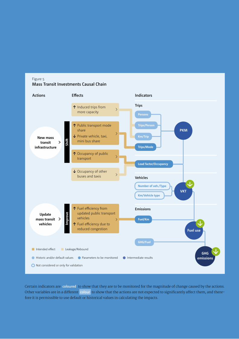
Figure 5
Mass Transit Investments Causal Chain
Actions Effects Indicators
New mass transit
infrastructure
Update mass transit
vehicles
↑ Induced trips from more capacity
↑ Occupancy of public transport
↑ Public transport mode share
↓ Private vehicle, taxi, mini bus share
↑ Fuel efficiency from updated public transport vehicles
↑ Fuel efficiency due to reduced congestion
↓ Occupancy of other buses and taxis
Trips
Vehicles
Emissions
Shift
Impr
ove
PKM
Load factor/Occupancy
Number of veh./Type
Persons
Trips/Person
Km/Trip
Trips/Mode
Km/Vehicle typeVKT
GHG emissions
Fuel use
Intended effect Leakage/Rebound
Historic and/or default values Intermediate resultsParameters to be monitored
Fuel/Km
GHG/Fuel
Not considered or only for validation
Certain indicators are coloured to show that they are to be monitored for the magnitude of change caused by the actions.
Other variables are in a different colour to show that the actions are not expected to significantly affect them, and there-
fore it is permissible to use default or historical values in calculating the impacts.

Compendium on GHG Baselines and MonitoringPassenger and freight transport
26
Determining the baseline and calculating emission reductions
Analysis approach
There are often multiple options for determining the
baseline and mitigation scenarios which are needed for
analysing the effects of a selected mitigation action type.
Some mitigation action types will require a specific anal-
ysis approach while others may be more flexible. Ex-ante
and ex-post analysis usually have different needs for pro-
jections and forecasts versus collection of existing data.
This section discusses the typical approaches.
Uncertainties and sensitivity analysis
This section gives an overview of which variables are
least certain and discusses the level of sensitivity the fi-
nal results may show due to that uncertainty.
Guidance on the selection of analysis tools for the mitigation action type
Depending upon the mitigation action type, certain key
variables may need to be highly disaggregated to achieve
good accuracy in estimation while others may not. The
section contains a table listing the variables specific to the
mitigation action type by level of accuracy. e.g.,
· Lower accuracy: lists aggregated variables
· Medium accuracy: lists partially disaggregated variables
· Higher accuracy: lists highly disaggregated variables
The navigation map is a graphic representation of the
range of tools that are currently available for analysing
the mitigation action type. The names of specific software
tools, CDM methodology documents and other works that
address GHG reduction analysis for the mitigation action
type is superimposed upon the map of analysis purposes
and accuracy levels. The navigation map should be used as
a basic guide for selecting available analysis methodolo-
gies and tools based on the availability of accurate data and
the objective of the analysis. The underlying categories are
shown in Figure 6.
The last part of the navigation section presents a fuller de-
scription of the various tools shown in the map, including
a qualitative estimation of the level of effort and technical
capacity required to use various types of tools, and a table
summarizing further details of specific tools in each type,
grouped into general categories based on the methodolog-
ical approach and the navigation map.
Monitoring
Monitoring involves the collection of indicator data per-
taining to the mitigation action. It is the first step in the
Monitoring, Reporting and Verification (MRV) process.
Specifics of monitoring will depend on many factors, in-
cluding data availability, policy commitments, donor
agreements, etc. A basic three level method of monitoring
is suggested as a starting point for developing individual
monitoring schemes, using Implementation, Performance
and Impact level variables. A table will present a minimum
list of key variables and recommended intervals for meas-
urement if no other requirements are present, (e.g., more
frequent interval may be required for CDM).
Although monitoring is only the first step of MRV, this
volume does not focus on reporting or verification. Re-
porting structures are often agreed to with a donor or fi-
nance provider, such as a bank or NAMA funder. National
programmes may contain monitoring arrangements in-
cluded in the legislation or directive. Other circumstanc-
es may require reporting to be aligned with national re-
porting structures for international commitments. For
verification, cross checking with fuel sales data and other
national or international values and historical results can
be done to provide confidence. CDM and NAMA verifica-
tion may require independent third party review. Rigorous
verification can also include spot checks of data sources.
In all cases, good documentation is key to verification, in-
cluding transparency about assumptions used in the BAU
or baseline scenario, references to sources of default data
and documentation that proper statistical procedures were
followed (e.g. survey guidelines).
Example
A brief synopsis and a link to further materials for a case
study of an analysis of a mitigation action within the mit-
igation action type that is ongoing or has been completed.

Compendium on GHG Baselines and MonitoringPassenger and freight transport
27
Figure 6
Navigating classes of available methods and associated tools actions
Prioritize policies
Objective
Report results
Mitigation planning
Emissions trading
Ex-a
nte
Lower accuracy Medium accuracy Higher accuracy
Expert judgment
Spreadsheet tools with defaults
Travel demand models
CDM methodologies
Other bottom-up methodologies/
guidance
Spreadsheet tools with local
data
Historic local trends
Ex-p
ost

Compendium on GHG Baselines and MonitoringPassenger and freight transport
28
Chapter 1
MASS TRANSIT INVESTMENTS

Compendium on GHG Baselines and MonitoringPassenger and freight transport
29
1.1 DESCRIPTION AND CHARACTERISTICS OF MASS TRANSIT INVESTMENTS
This mitigation action covers project level investments
that create or extend specific mass transit passenger
transport infrastructure in a region. This includes bus
rapid transit (BRT), tram, metro, cable cars etc. These
actions expand the capacity, frequency, speed and/or
coverage of public transport with the goal to increase its
mode share while decreasing the mode share of less effi-
cient modes, especially private vehicles. Secondary goals
are to increase per vehicle occupancy of public transport,
update the vehicles and improve traffic flow.
The outcomes of successful implementation of this miti-
gation action are expected to increase the mode share of
public transport to reduce the VKT of private vehicles, and
increase the overall efficiency of public transport, lead-
ing to reduced GHG emissions through lower overall VKT
and transport energy use in the region. Mass transit in-
vestments are known to generate a number of sustainable
development co-benefits, which may include access to af-
fordable mobility, shorter travel times and reduced acci-
dents. It can also encourage more compact urban develop-
ments with increased non-motorized travel, reduced auto
ownership and improved health outcomes due to more
opportunities to exercise and lower pollution levels.
1.2 STRUCTURE OF MITIGATION EFFECTS
1.2.1 Cause-impact chain
Mass transit investment actions should result in meas-
urable effects that are reflected in certain indicators in
bottom-up models (ASIF approach). The expected chang-
es in those variables will cause the desired outcomes. See
Figure 7.
1.2.2 Key variables to be monitored
The key variables that are expected to change by mass
transit investment are listed below, followed by the ex-
pected mechanism that causes them to change. A given
project may not affect every variable if the appropriate
mechanism of change is not present. For example if up-
dating to more modern transit vehicles is not part of the
project, then the portion of change in vehicle occupancy
and fuel consumption due to modern vehicle technology is
not present. If no change from any other factor is expected
(e.g., speed), then historic/default values can be used.
1.2.3 Monitor for intended effects
· Mode shares - new, improved transit system will at-
tract travellers from other modes
· Vehicle occupancy of modes – new transit vehicles will
have more capacity than old vehicles and will be more
utilized
· Fuel efficiency of new vehicles – new transit vehicles
will employ more efficient technology and have diffe-
rent fuel consumption and/or different drive technolo-
gies, including self-driving vehicles
· Traffic speeds – congestion will decrease leading to hi-
gher average travel speeds which can affect fuel con-
sumption of all modes
1.2.4 May be monitored for leakage or rebound effects
· Trips - induced trips can be created by the increased
total transport capacity (negative rebound effect), this
could include NMT trips shifting to create new vehicle
transport trips
· Trip length – increased capacity can sometimes lead to
longer trip lengths because the induced trips have more
distant origins or destinations
· Reduced occupancy of other modes – competing modes
such as taxis may see reduced numbers of passengers
resulting in lower occupancy
Chapter 1Mass Transit Investments

Compendium on GHG Baselines and MonitoringPassenger and freight transport
30
Figure 7
Mass transit investments Causal Chain
Actions Effects Indicators
New mass transit
infrastructure
Update mass transit
vehicles
↑ Induced trips from more capacity
↑ Occupancy of public transport
↑ Public transport mode share
↓ Private vehicle, taxi, mini bus share
↑ Fuel efficiency from updated public transport vehicles
↑ Fuel efficiency due to reduced congestion
↓ Occupancy of other buses and taxis
Trips
Vehicles
Emissions
Shift
Impr
ove
PKM
Load factor/Occupancy
Number of veh./Type
Persons
Trips/Person
Km/Trip
Trips/Mode
Km/Vehicle typeVKT
GHG emissions
Fuel use
Intended effect Leakage/Rebound
Historic and/or default values Intermediate resultsParameters to be monitored
Fuel/Km
GHG/Fuel
Not considered or only for validation
1.2.5 Interaction factors
The magnitude of change in the key variables will be
affected by the specific characteristics of the mass tran-
sit investment and also by other contextual factors. To
achieve the best effects, the mitigation action must be
tailored to the specific context in each city. Some metho-
dologies, travel demand models for example, may be able
to quantitatively account for certain contextual factors.
For other methods a qualitative assessment using expert
judgment may be needed. When performing ex-ante es-
timation of the mitigation potential of a mass transit ac-
tion, the following factors can have a substantial impact
Chapter 1Mass Transit Investments

Compendium on GHG Baselines and MonitoringPassenger and freight transport
31
on magnitude and should be taken into account:
· Quality (travel time, comfort, convenience, etc.) and
fare structure of the new public transport lines
· Potential for improved overall travel conditions in co-
rridor (e.g., level of congestion)
· Land use density and diversity in corridor
· Parking availability in corridor
· Pedestrian and bicycle infrastructure
· Transit-supportive land use plans (TOD, parking, pe-
destrian access)
1.2.6 Boundary setting
New transit lines can draw riders from within walking
distance of the corridor, but also via other modes such as
bicycle or park and ride from within a larger ride shed. In
the longer term, new transit can affect the urban form
of an entire city, so the boundary could be as large as
the urban area. Boundary will depend upon the size of
the project and on data availability; larger geographical
boundaries for analysis can capture more interaction and
temporal effects but will require greater data collection
costs. Methodologies for urban programmatic actions
may become useful if the scope of the project is quite lar-
ge or includes multiple transit lines. (See action type 2)
Upstream emissions from electricity generation should
be included if the transit system is powered electrically.
However if the mitigation action of the project aims so-
lely at the switch to electric energy, that is if the mass
transit line is part of the baseline and the only difference
is energy source, then the analysis should consider me-
thodologies under Fuel switching (action type 4).
Large projects such as new subways may have substan-
tial construction emissions, which should be considered
as part of the lifecycle emissions and factored into calcu-
lations. In this case it may be necessary to also calculate
baseline construction emissions if the BAU scenario in-
cludes large roadway or other construction projects.
1.2.7 Key methodological issues
The GHG impact depends on the specific characteristics
of the transit line and surrounding land uses, so collec-
tion of local variables becomes important. Variables per-
taining to the operational characteristics of the old and
the new line such as length, current ridership and fuel
use of transit vehicles, are usually known or can be ob-
tained without too much difficulty. Future land uses can
be forecast based on trends and planning documents.
The main difficulty is in developing a calibrated model of
the effect of these variables on ridership to estimate how
much the project will attract new riders, change the mode
share and reduce private vehicle VKT. Many existing tools
Table 2
Dimensions of boundary setting for mass transit investment mitigation actions
Dimension Options for boundary setting
Geographical
Temporal
Upstream/downstream
Transport sub-sector
Emissions gasses
Corridor, ride shed, urban area Temporal
10 – 50 years Upstream/downstream
Energy sector (electricity, biofuels), may also consider
infrastructure construction Transport sub-sector
Passenger transport, public transit Emissions gasses
CO2eq (may include CH4, N2O)
Chapter 1Mass Transit Investments

Compendium on GHG Baselines and MonitoringPassenger and freight transport
32
contain models that range in complexity and their use of
default values versus user supplied values. Specific issues
to consider when selecting a methodology include:
· Establishing a clear causal chain between new transit
line and measurable effects: Determine if the effects
could have occurred without the new investment.
· Estimating mode shares and potential new riders, es-
pecially ex-ante: Account for the influence of new land
uses, costs of travel and other factors.
· Determining if new transit ridership (PKM) will increa-
se transit VKT or increased occupancy will reduce tran-
sit VKT.
· Data availability on trip length by mode: Are recent lo-
cal data available?
· Estimating rebound effects – induced trips for public
transport and private modes if project increases total
capacity: Is this effect expected to influence results?
· Availability of disaggregated emissions factors for old
and new vehicle types and at BAU and mitigation sce-
nario speeds
1.2.8 Double counting concerns
Other policies and actions taken to mitigate GHG may
have synergistic or interaction effects on a mass transit
mitigation action. This can lead to difficulty in attribu-
ting the reduction to a particular action or to counting the
same tonnes more than once for different actions. Care
should be taken in this regard if any of the following po-
licies or actions is being implemented concurrently with
mass transit lines. In some cases a dynamic baseline
could account for the effect; in other cases it may be be-
tter to analyse the combined effect of the actions rather
than trying to disaggregate the reductions. (See action
type 2 urban programmatic actions.)
1.3 DETERMINING THE BASELINE AND CALCULATING EMISSION REDUCTIONS
1.3.1 Analysis approach
The baseline scenario for mass transit investments can
be described as “Passengers are transported using a di-
verse transport system involving buses, trains, cars,
non-motorized transport modes, etc. operating under
mixed traffic conditions and possibly using older, less-ef-
ficient vehicles.” Baseline emissions are estimated by de-
termining the passenger kilometres (PKM) of each mode,
Table 3
Actions with potential for double counting for mass transit investment mitigation actions
Mitigation action May affect this variable
Fuel switching (e.g., subsidies for specific fuel types)
Fuel cost (taxes or subsidy removal)
Vehicle fuel efficiency improvements (e.g., emission standards)
Parking pricing
TOD policies (promote additional mode shift)
GHG emission factor per unit fuel
Mode share
Fuel efficiency, mode share
Mode share
Induced trips, mode share
Chapter 1Mass Transit Investments
Compendium on GHG Baselines and MonitoringPassenger and freight transport
33
converting them into vehicle kilometres travelled (VKT)
by the vehicle type each mode uses and applying an ap-
propriate emission factor.
Current travel data serves as the basis for this baseline
calculation, which must then be projected into the future
for ex-ante analysis and “counterfactually projected” for
ex-post analysis. Any mass transit investment project
should be considered to create a new mode within the
study area that alters the distribution and amount of VKT
among modes. Ex-ante analysis requires a future projec-
tion of this scenario to compare to the baseline scenario.
The most rigorous method for ex-ante analysis, travel
demand models, makes future estimates of trips, PKM
and VKT for all modes based on spatial interactions be-
tween origin and destination locations from local land
use. Travel models provide this travel activity input to
separate emission factor models to calculate the final
GHG impacts. Other methodologies estimate some or all
travel activity variables using one of the three methods
described below, and apply default values for remaining
variables. Some older methodologies focus on the pro-
jection of passenger trip shares and use defaults for the
calculation of PKM and conversion to VKT.4
There are three general approaches for projecting or
counterfactually projecting travel activity for baselines
or mass transit investment scenarios:
· Travel demand models – generally used for ex-ante
analysis of BAU or mitigation scenarios.
· Travel activity survey – ex-post is usually done with
MRT project passengers, comparing alternative modes
to the real situation of using the MRT. Ex-ante can do
a stated preference survey to estimate future ridership
· Expert judgment based on historical trends, using time
series data gathered ideally for at least 10 years – can be
used for ex-ante projection or ex-post counterfactually
projecting situations.
Ex-post analysis also requires estimates of current emis-
sions, which are calculated based on the current tran-
sit ridership and traffic counts and respective emission
factors within the defined boundaries. Most methodolo-
gies focus on the new riders of the mass transit project.
Emission reductions, as always, are the difference be-
tween the project emissions (real or estimated ex-ante)
and the baseline. Methodologies may vary as to whether
upstream emissions from fuel production are considered.
These emissions can be a factor if the new transit project
uses different fuels or substantially greater fuel than the
baseline.
1.3.2 Uncertainties and sensitivity analysis
The most uncertain variable in the emission reduction
analysis of a mass transit system is usually the ex-ante
estimate of mode split and new ridership. Because it de-
pends on the relative attractiveness of the mass transit
system versus the previously available modes for each in-
dividual rider, it can be hard to estimate. Travel demand
models offer the most sophisticated option, but even then
there can be a range of error due to input uncertainty.
Ex-post methodologies all have characteristic uncertain-
ties. Survey methods can introduce the subject’s personal
biases as they ask users to state future preference or im-
agine a counterfactual scenario. Historical methods start
with past data but must assume that no critical changes
will be introduced. As mentioned, travel models require
projections of future growth as inputs to the model,
which is a source of uncertainty for that methodology.
The potential for rebound effects such as induced trips or
changes in trip lengths in some modes can be significant.
The associated uncertainty can be high if there are no
previous experiences in the city/country to draw analysis
from, as this effect is very culturally and locally specific.
4 See <http://www.apta.com/resources/hottopics/sustainability/Documents/Quantifying-Greenhouse-Gas-Emissions-APTA-Recommended-Practices.pdf>
Chapter 1Mass Transit Investments

Compendium on GHG Baselines and MonitoringPassenger and freight transport
34
1.4 DETERMINING THE BASELINE AND CALCULATING EMISSION REDUCTIONS
Higher degrees tof accuracy can be obtained with more
disaggregated data, if some or all data is locally derived.
While combining local data with defaults can yield bene-
fits, using disaggregated default data alone is seldom more
accurate than aggregated default data. For example, highly
disaggregated emissions factors for various types of vehi-
cles at different speeds are available. Using these factors
without accurate values for trip length, mode share and
Table 4
Level of disaggregation of key variables for mass transit investment mitigation actions
Lower accuracy Medium accuracy
Degree of local data disaggregation
Higher accuracy
Travel activity data
Emission factors
• Total vehicle trips
• Forecast change in transit
ridership
• Average occupancy of
Privately Owned Vehicles
and transit vehicles*
• Average trip length*
• Average emission rates *
• Vehicle trips in boundary area by
vehicle type
• Vehicle trip length by vehicle type
• Proposed change in transit VKT from
operations (by vehicle type)
• Traffic speeds in corridor by vehicle
type (and time of day)
• Forecast travel speeds by vehicle
type after strategy implementation
• Forecast change in transit ridership
• Trip lengths of new transit trips*
• Prior mode shares of new transit
riders*
• Emission factors by vehicle type
• Emission rates by speed*
• Emission rates for new transit
vehicles (by speed)*
• Person trips in boundary area by
vehicle type
• Person trip length by vehicle type
• Occupancy by vehicle type
• Proposed change in transit VKT from
operations (by vehicle type)
• Traffic speeds in corridor by vehicle
type (and time of day)
• Forecast travel speeds by vehicle type
after strategy implementation
• Forecast change in transit ridership
• Trip lengths of new transit trips
• Prior mode shares of new transit riders
• Adjustment for induced traffic due to
lower congestion*
• Forecast change in private vehicle VKT
by vehicle type (modelled)**
• All data items by time of day**
• Emission factors for new transit
vehicles (by speed)
• Current and future (or improvement
factor) emission rates by vehicle type
and speed
• Factors by emission gas or particle
type*
• Construction emission of new transit
vehicles and infrastructure**
*=default OK, **= optional item
Chapter 1Mass Transit Investments

Compendium on GHG Baselines and MonitoringPassenger and freight transport
35
fleet composition yields little improvement in accuracy
over using average, aggregated factors. Table 4 shows the
disaggregated data that is desirable for each general level
of accuracy.
Mass transit actions have a long history of in-depth anal-
ysis, such as ex-ante investment grade demand forecast
studies using travel demand models and the detailed
methodologies developed for ex-post emissions credit-
ing (e.g., CDM). More recently a number of sketch plan-
ning tools have also been developed for rapid assessment
of the potential GHG reductions that might be obtained
from new transit projects and other similar programs
that expand public transport capacity.
Figure 8 maps existing methodologies and tools for mass
transit investments according to their purpose (y axis)
and level of accuracy (x axis).
4 See <http://www.apta.com/resources/hottopics/sustainability/Documents/Quantifying-Greenhouse-Gas-Emissions-APTA-Recommended-Practices.pdf>
Chapter 1Mass Transit Investments
Figure 8
Navigating classes of available methods and associated tools for mass transit investment mitigation actions
Prioritize policies
Objective
Report results
Mitigation planning
Emissions trading
Ex-a
nte
Lower accuracy Medium accuracy Higher accuracy
Ex-p
ost
Spreadsheet or software tool Guidance document
Spreadsheet tools with defaults
BRT – TEEMP
Metro – TEEMP (sketch)
CCAP Emissions Guidebook
Emission Reduction Volume Calculator for BRT Project
Spreadsheet tools with local data
BRT – TEEMP (full)
Metro – TEEMP (full)
CDM methodologiesACM0016: Mass Rapid Transit Projects
AM0031: Bus rapid transit projects
AMS-III.U.: Cable Cars for MRTS
Tool 18: Baseline emissions for modal shift measures in urban passenger
transport
Other bottom-up methodologies/
guidanceWRI GHG Protocol Policy
and Action Standard: Road transport: BRT example
Travel modelsCube, TransCad, Visum,
Tranus, + Local emissions models, e.g., HBEFA,
MOVES
Modeshift from BRT

Compendium on GHG Baselines and MonitoringPassenger and freight transport
36
1.4.1 Description of tool types
The following sections describe a number of tools that
are available for estimating GHG reduction from transit
projects. They are classified according to similarities in
methodology.
1.4.2 Travel demand models
These are spatial interaction models that calculate VKT
disaggregated by mode, time of day and speed. Trip
lengths are based on location of origins and destina-
tions. Mode choice can be modelled based on interaction
of origins, destinations and transport systems. Induced
trips can be modelled using capacity restraint formula
(activity models may have more sophisticated methods).
With appropriate sub modules some models can include
freight, transit, NMT. Some models can include land use
simulations as well. Important disaggregated variables
cascade through analysis. Some defaults may be includ-
ed and models include the ability to change any variable.
Models are calibrated by entering local data from detailed
travel surveys and comparing the model output to known
results. This option is the most accurate choice for fore-
casting future travel activity parameters.
Typically, highly disaggregated activity data from travel
demand models is input to a separate emissions mod-
el calibrated to national or supra-national fleets. Some
software packages incorporate emissions factors from
various sources for an extra cost. External standard
emissions models that accept highly disaggregated in-
puts include MOVES, HBEFA, etc. (Highly disaggregated,
e.g., speed sensitive, emissions models are discussed un-
der Mitigation Action type 8.) Emissions models also have
to be adapted to local or at least country-specific circum-
stances regarding e.g., the underlying fleet composition
and emission factors to deliver meaningful results. Trav-
el model outputs can, however, also be aggregated and
emissions calculated with simpler emissions factors.
Table 5
Travel demand models for mass transit investment mitigation actionsEase of use/data collection: Highly resource and data intensive
Name Application /summary
Scope Computer based
Methodology documentation
Defaults Provided
Data collection guidance
Cost of tool
Cube
TransCad
VISUM
EMME
Tranus
Land use
module available
Emissions
module available
Emissions
module available
No other
modules
No other
modules
Excellent
Excellent
Excellent
Excellent
Very good
Internal
parameters*
Internal
parameters*
Internal
parameters*
Internal
parameters*
Internal
parameters*
Travel activity
Travel activity
Travel activity
Travel activity
Travel activity
and land use
Yes
Yes
Yes
Yes
Yes
Paid training
offered
Paid training
offered
Paid training
offered
Paid training
offered
Fair
High
High
High
High
Free
*For example friction factors, mode choice curves, and other coefficients for internal sub-models
Chapter 1Mass Transit Investments

Compendium on GHG Baselines and MonitoringPassenger and freight transport
37
Table 6
Disaggregated bottom-up ex-post guidance for mass transit investment mitigation actionsEase of use/data collection: Moderately resource and data intensive
Name Application /summary
Scope Computer based
Methodology documentation
Defaults Provided
Data collection guidance
Cost of tool
ACM0016: Mass Rapid Transit Projects
AM0031: Bus rapid transit projects
AMS-III.U.: Cable Cars for MRTS
WRI GHG Protocol Policy and Action Standard: Transport sector guidance 2
Modeshift from BRT
CDM 18:Baseline emissions for modal shift measures in urban passenger transport
Ex-post focus;
Leakage: bus and taxi
occupancy change,
congestion effect on
fuel efficiency and in-
duced trips, upstream
emissions of gaseous
fuels
Ex-post focus;
Leakage: bus and taxi
occupancy change,
congestion effect on
fuel efficiency and in-
duced trips, upstream
emissions of gaseous
fuels
Ex-post focus;
Leakage: general
guidance to consider,
occupancy guidance
for upstream emis-
sions of electricity
Ex-ante or ex-post;
Guidance on setting
boundaries and
selecting level of detail,
identifying first, second
and third order effects
General PKM method-
ology; refers to the first
three CDM methodolo-
gies above
Ex-post focus;
General PKM meth-
odology
Leakage: general
guidance only
Excellent
Excellent
Excellent
Very good
Good
Excellent
Technology
improvement
factor
Capacity restraint
factor
IPCC upstream
fuel emissions
factors
Technology
improvement
factor
Capacity restraint
factor
IPCC upstream
fuel emissions
factors
Technology
improvement
factor
IPCC upstream
fuel emissions
factors
Examples of
baseline vehicle
emissions factors
None
Technology
improvement
factor
Global defaults
for vehicle occu-
pancy, fuel effi-
ciency, electricity
consumption
Project activities
that establish
and operate an
MRTS without
feeder lines
Construction
and operation
of a new BRT
or replacement
or expansions
of existing BRT
(adding new
routes and lines)
New cable
car passenger
transport
Uses BRT as
example of how
to apply protocol
New BRT
projects
Activities in
urban passenger
transport that
implement
a measure
or a group of
measures aimed
at a modal shift
to urban public
transit such as
metro, bus rapid
transit (BRT), light
rail and trams
No
No
No
No
No
No
Excellent
Includes
survey
template and
guidance
Excellent
Includes
survey
template and
guidance
Excellent
Includes
survey
template and
guidance
Good;
guidance on
develop-ing
monitor-ing
plans
Poor
Fair, general
guidance on
paramet-ers to
collect
Free
Free
Free
Free
Free
Free
Chapter 1Mass Transit Investments
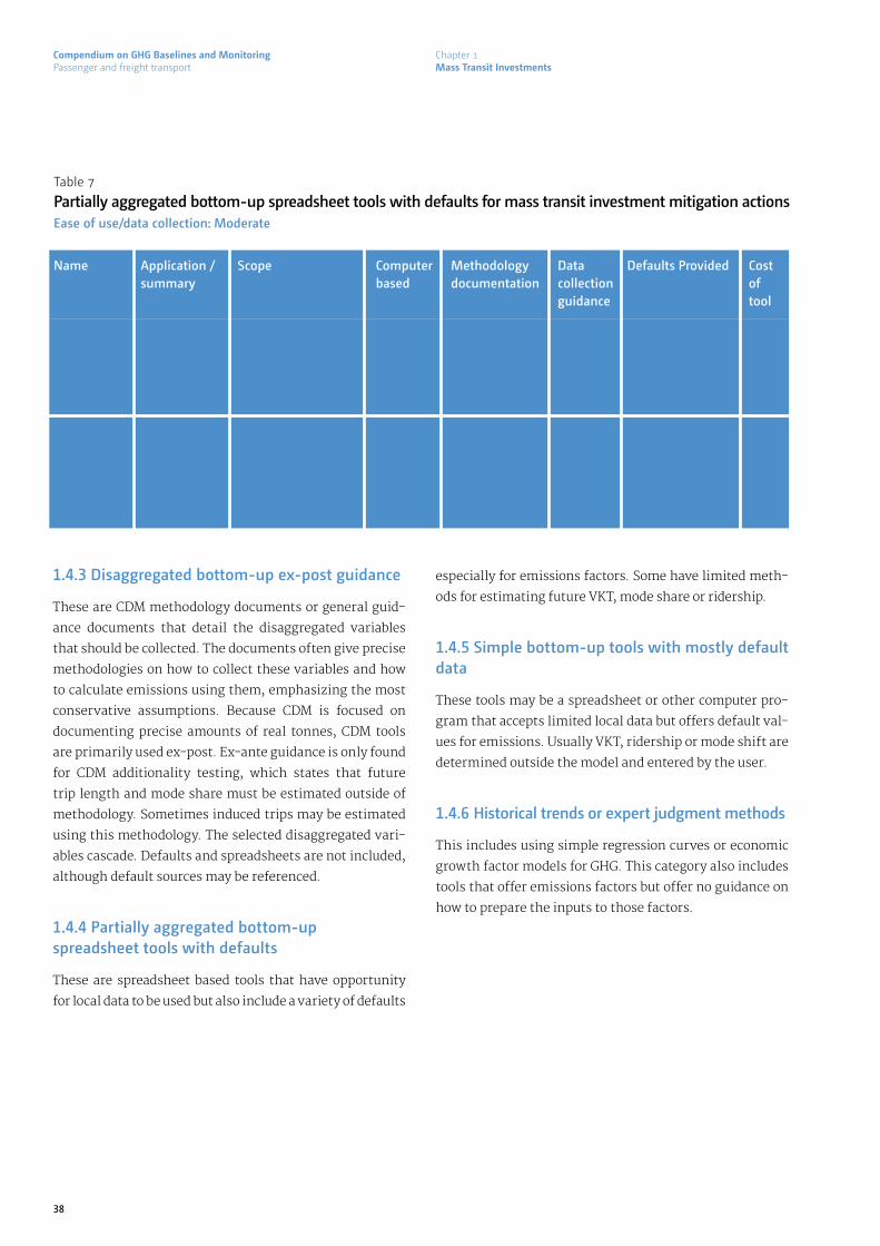
Compendium on GHG Baselines and MonitoringPassenger and freight transport
38
Table 7
Partially aggregated bottom-up spreadsheet tools with defaults for mass transit investment mitigation actionsEase of use/data collection: Moderate
Name Application /summary
Scope Computer based
Methodology documentation
Defaults ProvidedData collection guidance
Cost of tool
BRT-TEEMP (full)
Metro-TEEMP (local data)
Ex-ante focus; includes
BRT mode shift estimation
if local data available;
includes co-benefits
estimation
Ex-ante city-wide; requires
local data on mode shift
for best accuracy; includes
land use effect factor;
includes construc-tion life
cycle emissions estimator
Good
Good
Fuel efficiency by speed
Occupancy
Trip length
Fuel emission factors
Construction factors
Fuel efficiency by speed
Occupancy
Trip length
Fuel emission factors
Construction factors
New or
expanded BRT
system
New or expanded
Metro system
(fixed rail)
Yes
Yes
Fair
Fair
Free
Free
1.4.3 Disaggregated bottom-up ex-post guidance
These are CDM methodology documents or general guid-
ance documents that detail the disaggregated variables
that should be collected. The documents often give precise
methodologies on how to collect these variables and how
to calculate emissions using them, emphasizing the most
conservative assumptions. Because CDM is focused on
documenting precise amounts of real tonnes, CDM tools
are primarily used ex-post. Ex-ante guidance is only found
for CDM additionality testing, which states that future
trip length and mode share must be estimated outside of
methodology. Sometimes induced trips may be estimated
using this methodology. The selected disaggregated vari-
ables cascade. Defaults and spreadsheets are not included,
although default sources may be referenced.
1.4.4 Partially aggregated bottom-up spreadsheet tools with defaults
These are spreadsheet based tools that have opportunity
for local data to be used but also include a variety of defaults
especially for emissions factors. Some have limited meth-
ods for estimating future VKT, mode share or ridership.
1.4.5 Simple bottom-up tools with mostly default data
These tools may be a spreadsheet or other computer pro-
gram that accepts limited local data but offers default val-
ues for emissions. Usually VKT, ridership or mode shift are
determined outside the model and entered by the user.
1.4.6 Historical trends or expert judgment methods
This includes using simple regression curves or economic
growth factor models for GHG. This category also includes
tools that offer emissions factors but offer no guidance on
how to prepare the inputs to those factors.
Chapter 1Mass Transit Investments

Compendium on GHG Baselines and MonitoringPassenger and freight transport
39
Table 8
Simple bottom-up tools with mostly default data for mass transit investment mitigation actionsEase of use/data collection: Moderate to low
Name Application /summary
Scope Computer based
Methodology documentation
Defaults ProvidedData collection guidance
Cost of tool
BRT-TEEMP (sketch)
Metro-TEEMP (default data)
CCAP Emissions Guidebook
Ex-ante focus; includes
BRT mode shift estima-
tion based on defaults;
includes co-benefits
estimation
Ex-ante city-wide focus;
offers default mode shift
choices; includes land
use effect factor; includes
construction life cycle
emissions estimator
Ex-ante tool; sketch plan-
ning estimates based on
combining local data and
defaults; Includes fuel cost
savings calculator
Good
Good
Good
Fuel efficiency by speed
Occupancy
Trip length
Fuel emission factors
Construction factors
Fuel efficiency by speed
Occupancy
Trip length
Fuel emission factors
Construction factors
Rules of thumb based
on case studies
New or expanded
BRT system
New or expanded
Metro system
(fixed rail)
New or expanded
BRT/ Metro
system
Yes
Yes
Yes
Fair
Fair
Fair
Free
Free
Free
Chapter 1Mass Transit Investments
Table 9
Historical trends or expert judgment tools for mass transit investment mitigation actionsEase of use/data collection: Low
Name Application /summary
Scope Computer based
Methodology documentation
Defaults ProvidedData collection guidance
Cost of tool
Emission Reduction Volume Calculator for BRT Project
Requires user to input all
travel data except default
emission factors; calcu-
lates total emissions and
reductions
Fair Bus emission factors
by vehicle type;
construction emission
factors
New or expanded
BRT system
Yes Poor Free

Compendium on GHG Baselines and MonitoringPassenger and freight transport
40
1.5 MONITORING
Performance of the mitigation action can be monitored
by tracking key variables over time. The monitoring fre-
quency will vary, depending on the monitoring regimen
and the budget available for data collection. CDM meth-
odologies generally require annual monitoring. National
level biennial update reports (BUR) are submitted every
two years to the UNFCCC but may not need the most pre-
cise project level data. Key mode share and trip length
data can require transport surveys that may not be possi-
ble on an annual or biannual basis. Although new meth-
ods such as mobile phone tracking can substitute for sur-
veys in some instances, many organizations cannot be
assumed to have reliable data for all variables annually.
However different variables can be updated at different
intervals. Transit ridership data is usually collected reg-
ularly so that annual monitoring is possible, even if trip
length, etc. are only updated every few years.
It is also suggested that information on implementation
and performance be included in the monitoring plan to
show progress before the full effects of the action may be
apparent. Table 10 presents a minimum list of key var-
iables and recommended maximum intervals for meas-
urement if no other requirements are present, (e.g., more
rigorous requirements are often in place for CDM).
1.6 EXAMPLE − COLOMBIA TRANSMILENIO
The Colombia Transmilenio CDM project was registered in
2006 for a seven year crediting period. During this time
the procedures of “Baseline Methodology for Bus Rapid
Table 10
Minimum indicator set for mass transit mitigation action
Category Indicator Normal monitoring frequency
Implementation indicator
Performance indicators
Impact indicators
Construction and operation of new transit line
Ridership on new line
Traffic in corridor
Calculated passenger transport VKT by mode
Latest emission rates by mode
Calculated emissions in study area
One time or by construction phase
Annual
Annual
5 years
5 years
5 years
Chapter 1Mass Transit Investments

Compendium on GHG Baselines and MonitoringPassenger and freight transport
41
Transit Projects” AM0031 were used to monitor the effects.
There were a total of seven monitoring reports issued.
The Methodology was refined slightly during the seven
years but generally consisted of collecting fuel consump-
tion data, VKT data and passengers carried data from the
TransMilenio system operators to calculate the mitigation
scenario. The counterfactual baseline scenario was calcu-
lated each year by a series of surveys of passengers which
queried them about the mode, number and length of trips
they would have taken “in the absence of TransMilenio”.
Leakage and life cycle parameters were also measured.
This included construction emissions for periods of ex-
pansion, emissions from bus manufacturing as well as
the possible effects of reduced congestion on induced
travel. For years 3 and 7 emissions due to reduced load
factors of other buses and taxis were also included. Gen-
erally the load factor leakage was found to be negligible.
At the last reporting period the actual GHG emission reduc-
tions for that year were found to be 80, 128 tCO2e as com-
pared to the ex-ante estimate of 307,300 tCO2e. According
to the original CDM Project Design Document all Phase III
trunk routes as well as two routes of Phase IV should have
been operational by 2012. However these suffered delays
due to various reasons including re-planning of routes
based on experience with Phase II as well as on-going dis-
cussions about BRT versus a rail-based Mass Rapid Transit
System. Due to the low demand for carbon credits and the
less than expected amount of reductions, the project was
voluntarily withdrawn from the CDM in 2014.
Further details are available at:
https://cdm.unfccc.int/Projects/DB/DNV-CUK1159192623.07/
view?cp=1
Chapter 1Mass Transit Investments

Compendium on GHG Baselines and MonitoringPassenger and freight transport
42
Chapter 2
COMPREHENSIVE URBAN TRANSPORT PROGRAMMES AND PLANS
Compendium on GHG Baselines and MonitoringPassenger and freight transport
43
2.1 DESCRIPTION AND CHARACTERISTICS OF URBAN TRANSPORT PROGRAMMES AND PLANS
This mitigation action covers programmes and plans
that coordinate planning, investment and policy to re-
duce motorized VKT through activity reduction and/
or mode change in urban transport. Some programmes
also include measures to improve vehicle efficiency or
promote alternative fuels; if they are a major part of the
programme, their individual effects are better addressed
through methodologies in chapter 6 or 7. Comprehen-
sive urban transport mitigation actions can range from
national level programmes to support sustainable urban
transport across the country to regional or local plans
that implement a range of strategies. National level pro-
grammes can be more centralised or more decentralised
depending upon the degree of autonomy given to the re-
gional or local authorities as they choose strategies and
projects (cf. Diaz and Bongardt, 2013).
The key characteristic that differentiates these pro-
grammes and plans from other mitigation actions is that
they support a range of potential measures that are inte-
grated and coordinated in order to achieve a synergistic
effect, so that, in the long term, travel is pushed away from
private vehicles and pulled toward sustainable modes such
as public transport and/or NMT. Some programmes also
address urban freight and city logistics. The specific ac-
tions within a given urban transport programme or plan
will vary between nations or regions depending upon the
particular emphasis. Although programmes and plans can
conceivably include any type of strategy, in general, these
mitigation actions improve accessibility of cities through
land planning and regulation promoting increased den-
sity and mixed uses, expand investment for non-motor-
ized and public transport, and may create disincentives for
private and commercial vehicle use by restricting parking
and road capacity or regulating access rights for freight
and delivery transport. Secondary goals may include mod-
ernizing transit vehicles and improving traffic flow.
The outcomes of successful implementation of these pro-
grammes and plans are expected to reduce the number of
motorized trips (passenger and freight), reduce the length
of trips and increase the mode share of non-motorized
and public transport to reduce the VKT of private vehicles,
and increase the overall efficiency of public transport,
leading to reduced GHG emissions through lower overall
VKT and transport energy use in the area of implemen-
tation. Comprehensive urban transport programmes and
plans are known to generate a number of sustainable de-
velopment co-benefits, which may include access to af-
fordable mobility, shorter travel times and reduced acci-
dents. They can also improve quality of life and sense of
place, increase economic returns on investments in mass
transit, reduce car ownership and improve health out-
comes due to more opportunities for physical activity and
lower pollution levels.
2.2 STRUCTURE OF MITIGATION EFFECTS
2.2.1 Cause-impact chain of urban transport pro-grammes and plans
The causal chain of comprehensive urban transport pro-
gramme and plan actions can encompass many interven-
tion points in a bottom-up model. The combined effects of a
package of avoid, shift and improve measures will result in
measurable changes in the indicators in bottom-up models
(ASIF approach) manifested at the level of the urban area.
The expected changes in those variables will cause the de-
sired outcomes in intermediate variables. Rather than focus
on the individual effects of single measures, methodolo-
gies for these types of action look at changes in indicators
or intermediate variables holistically. The advantage of this
method is that interactions and synergies are included in
the results; the disadvantage is that the effect of the indi-
vidual measures is not known, so it is difficult to learn which
measures within the package are most effective. See Figure
9 (illustrated for urban transport).
Chapter 2Comprehensive urban transport programmes and plans

Compendium on GHG Baselines and MonitoringPassenger and freight transport
44
2.2.2 Key variables to be monitored
Comprehensive urban transport programmes and plans
have the potential to change nearly any of the key varia-
bles in a bottom-up model. The variables are listed below,
followed by the expected mechanism that causes them to
change. Some methodologies focus on intermediate varia-
bles, especially VKT, in order to capture the overall effects
of a programme. A given project may not affect every var-
iable if the appropriate mechanism of change is not pres-
ent. Although a comprehensive programme or plan should
affect all the variables listed below, if no change from any
other factor is expected (e.g. speed), then historic/default
values can be used. For example if NMT or compact city
measures are not included, the number of motorized trips
per person might not be expected to change.
Figure 9
Comprehensive urban transport programmes and plans causal chain (passenger transport)
Actions Effects Indicators
Compact city design
Parking management
More cycling and walking investment
Update mass transit
vehicles
More Transit investment
Less Road investment
↓ (Motorized) trips/person
↓ Trip length
↑ Public transport mode share
↑ Occupancy of vehicles
↓ Share of other motorized modes
↑ Fuel efficiency of updated public transport vehicles
↑ Fuel efficiency of all modes due to reduced congestion
↑ Share of alternative fuel vehicles in public transport fleet
Trips
Vehicles
Emissions
Avo
idSh
iftIm
prov
eFu
el
PKM
Persons
Trips/Person
Km/Trip
Trips/Mode
Km/Vehicle typeVKT
GHG emissions
Fuel use
Intended effect
Historic and/or default values Intermediate resultsParameters to be monitored
Fuel/Km
GHG/Fuel
Load factor/Occupancy
Number of veh./Type
Chapter 2Comprehensive urban transport programmes and plans

Compendium on GHG Baselines and MonitoringPassenger and freight transport
45
2.2.3 Monitor for intended effects
· Trips/person – land use changes and NMT investment
may shift some trips to non-vehicle trips which can be
considered to reduce the (motorized) trips/person that
produce GHG emissions
· Km/trip – compact cities with increased density and
mixed use bring origins and destinations closer toge-
ther, reducing the length of necessary trips
· Mode shares - new, improved transit system may at-
tract travellers from other modes
· Vehicle occupancy of modes – new transit vehicles will
have more capacity than old vehicles and improved rou-
tes will be more fully utilized, ride sharing may increase
· Fuel efficiency of new vehicles – new transit vehicles
will employ more efficient technology and have different
fuel consumption and/or different drive technologies
· Traffic speeds – congestion may decrease leading to hi-
gher average travel speeds which can affect fuel con-
sumption of all modes
· Use of alternative fuels – some programmes may lead
to an increase in the fleet of vehicles using fuels with
lower carbon intensities
· Passenger kilometres – some methodologies may use
data at the PKM level, which would change based on in-
terventions affecting the variables above
· Vehicle kilometres travelled – some methodologies use
data at the VKT level, which would change due to inter-
ventions affecting the variables above
2.2.4 May be monitored for leakage or rebound effects [not shown in figure 9]
· Km/trip – there is some evidence that improving ove-
rall accessibility can lead to more long distance trips as
a rebound effect
· Construction emissions may need to be included for
major projects such as metro systems or new separated
bus lanes.
2.2.5 Interaction factors
Comprehensive mobility plans are by their nature inte-
grated strategies. Nevertheless, the magnitude of chan-
ges in the key variables will be affected by the specific
projects and characteristics of the urban transport pro-
gramme or plan used as mitigation action. To achieve the
best effects, the specific actions should be locally desig-
ned to best align with the political, economic, geographic
and cultural context of the urban area. National level
programmes are implemented through local or regional
plans to a greater or lesser extent depending upon the
degree of decentralization. Some methodologies may be
able to quantitatively account for certain contextual fac-
tors, while others may use default assumptions that are
applied to all cities under a programme. A qualitative as-
sessment using expert judgment may be needed to adjust
default factors. Especially when performing ex-ante es-
timation of the mitigation potential of a comprehensive
urban mobility programme or plan, the following ques-
tions should be considered:
· What are the expected GHG impacts of individual stra-
tegies included in the plan?
· What are the synergistic or antagonistic effects of the
combination of strategies included in the plan?
· Are legal authority, institutional arrangements, fun-
ding, etc. in place to implement the plan?
· Are there unique cultural, climatic, economic, geogra-
phic or other factors that may affect performance and
uptake of the strategies?
2.2.6 Boundary setting
Because these methodologies can be used for national
programmes or for regional or local plans, boundaries
will depend on the size of the project, i.e., the geographic
scope of the programme or plan. The expected changes
will be manifested at the level of the city or urban area,
so national scale programmes will use the methodologies
on a city by city basis and sum the expected results. When
analysing larger programmes it may be easier to use ave-
Chapter 2Comprehensive urban transport programmes and plans

Compendium on GHG Baselines and MonitoringPassenger and freight transport
46
rage data applied across all relevant cities, while for sma-
ller regional or local scale plans one should be sure that
local circumstances are properly reflected in the data,
although this may actually entail higher collection costs.
Upstream emissions from electric power generation mi-
ght need to be considered if the grid factor (emissions per
kilowatt) is substantial or if fuel switching measures are
included in the mitigation action.
Extensive programmes may have substantial construc-
tion emissions, which should be considered as part of the
lifecycle emissions and incorporated into ex-ante cal-
culations. In this case the mitigation scenario should be
compared to the baseline construction emissions of an
equivalent BAU mobility implementation.
2.2.7 Key methodological issues
The GHG impact depends not only the on scope of the
programme but also on how the design maximizes sy-
nergies among components. For this reason the key issue
is the level of detail of the analysis. Individual strategies
can be evaluated using specialized methodologies but a
simple summation of results from these methods can-
not be assumed because measures will interact in many
different ways to suppress, amplify or duplicate effects.
Broader sketch planning methods can provide order of
magnitude estimates that can be refined with individual
methodologies. Other specific issues to consider when
selecting a methodology include:
· What set of strategies will be considered the BAU sce-
nario? How will the new programme’s interactions and
synergies with current implementation pipeline be
considered?
· Is it clear how the programme or plan will be imple-
mented in the form of specific measures and regula-
tions?
· Data availability – What size statistically valid sample
is required to capture the entire effect of the mitigation
action?
· What level of accuracy is needed for ex-ante estima-
tion and for ex-post? Some simple inexpensive strategy
mixes can be assumed to produce directionally correct
results, while other, expensive packages of actions may
need to be evaluated more carefully for rebound effects
or other factors.
· How will land use changes affect travel activity?
2.2.8 Double counting concerns
Other policies and actions being implemented to mitiga-
te GHG may have synergistic or interaction effects with
the strategies within the urban mobility programme. Al-
though a comprehensive programme should include all
the actions within the boundary, national level actions
or local actions which are not in the programme need to
be considered. In addition, actions may have been taken
before the adoption of the programme that might change
Table 11
Dimensions of boundary setting for comprehensive urban transport programmes and plans
Dimension Options for boundary setting
Geographical
Temporal
Upstream/downstream
Transport sub-sector
Emissions gasses
National (sum of cities), regional, local
10 – 20 years, beyond 20 years
Energy sector (electricity, biofuels), infrastructure construction
Entire sector or applicable sub-sectors
CO2e (may include CH4, N2O )
Chapter 2Comprehensive urban transport programmes and plans

Compendium on GHG Baselines and MonitoringPassenger and freight transport
47
their expected results now that a programme is in pla-
ce. All these issues need to be carefully considered in the
establishment of the BAU scenario. For example, a new
subway line may be planned for construction before the
mitigation action is begun but it is also included as part of
the comprehensive urban mobility programme.
This can lead to difficulty in attributing the reduction the
comprehensive urban mobility programme or to counting
the same tonnes more than once or, conversely, not at-
tributing important reductions to the mitigation action.
Caution should be taken in this regard if any of the fo-
llowing policies or actions is being implemented concu-
rrently. Usually the expected effects of these policies can
be incorporated into a dynamic baseline.
2.3 DETERMINING THE BASELINE AND CALCULATING EMISSION REDUCTIONS
1.3.1 Analysis approach
Setting the baseline for evaluating a comprehensive ur-
ban mobility programme mitigation action is more chal-
lenging than for other types of actions. Because an ex-
isting mobility plan may already be in place, and parts of
it could be carried over to the new plan, it is necessary to
decide what aspects of the new plan are not in the BAU
and how they will interact with the rest of the plan. This
can be especially difficult if land use changes are contem-
plated. Travel demand models are the tools specifically
designed for evaluating comprehensive urban mobility
plans and remain the method of choice. However, the
cost, capacity and data requirements can be overwhelm-
ing, especially in less developed countries. For this rea-
son sketch models have been developed that allow easier
estimation of the ex-ante or ex-post effects. Also, since
comprehensive urban mobility programmes have not
been submitted under the CDM there are no UNFCCC ap-
proved methodologies to consider.
The baseline scenario for a given city level comprehen-
sive urban mobility plan can be described as the most
plausible continuation of current transportation invest-
ment and regulation plans and policies. As mentioned
above, there may be an existing plan that can be used, or
the current infrastructure can be “frozen” and a no-build
scenario considered.
Because there are so many potential interactions be-
tween strategies, baseline emissions are usually estima-
ted by determining the total overall vehicle kilometres
travelled (VKT) by the vehicle type within each mode
Table 12
Actions with potential for double counting for comprehensive urban transport programmes and plans
Mitigation action May affect this variable
National level fuel economy standards or fuel taxes
Previously planned transit infrastructure and service improvements
Previously planned non-motorized improvement
Pricing policies and strategies
TDM policies and strategies
Land use coordination with transport
No. of vehicles/type, fuel/km
Mode split, vehicle occupancy
(motorized) Trips per person
Mode split, vehicle occupancy, (motorized) trips per person
Mode split, vehicle occupancy, (motorized) trips per person
Mode split, vehicle occupancy, (motorized) trips per person
Chapter 2Comprehensive urban transport programmes and plans

Compendium on GHG Baselines and MonitoringPassenger and freight transport
48
and applying appropriate emission factors. Current tra-
vel data from counts and surveys serves as the basis for
this baseline calculation, which must then be projected
into the future for ex-ante analysis and counterfactually
projected for ex-post analysis. Ex-ante analysis requires
a future projection of the mobility plan scenario to com-
pare to the baseline scenario.
There are two general approaches that can be used for pro-
jecting or counterfactually projecting travel activity for
baselines or comprehensive urban mobility plan scenarios:
· Travel demand models –used for ex-ante analysis of
BAU or mitigation scenarios.
· Expert judgment based on historical trends, using time
series data gathered ideally for at least 10 years – can be
used for ex-ante projection or ex-post counterfactual
projection situations
Travel activity surveys are less useful in forecasting fu-
ture or counterfactual use of a comprehensive network
of transport infrastructure. While stated preference sur-
veys can be useful for a single proposed project, most
respondents cannot accurately describe how they would
choose among a variety of competing modes and routes
that do not yet exist.
Emission reductions, as always, are the difference be-
tween the project emissions (real or estimated ex-ante)
and the baseline. Consideration of upstream emissions
from fuel production or electricity may vary between me-
thodologies. These emissions can be a factor if any of the
included strategies uses different fuels or substantially
greater fuel than the baseline.
1.3.2 Uncertainties and sensitivity analysis
The most uncertain variable in the emissions reduction
analysis of a comprehensive urban mobility programme
mitigation action is usually the ex-ante estimate of mode
split and trip lengths. Sensitivity depends on the magni-
tude and relationship between the two variables, e.g., if
private vehicles have a smaller mode share but a long trip
length resulting in substantial VKT it may offset a transit
mode that is widely used but produces low VKT.
Ex-post methodologies also face uncertainty in estimat-
ing the counterfactual scenario, but historical data can
often be sufficient for this purpose, albeit with lower ac-
curacy. It is easier to compare the existing results of the
programme with known trends of historic BAU than to
accurately forecast the future results of a fundamentally
different programme.
2.4 GUIDANCE ON THE SELECTION OF ANALYSIS TOOLS FOR COMPREHENSIVE URBAN MOBILITY PROGRAMMES OR PLANS
Higher degrees of accuracy can be obtained with more
disaggregated data, if some or all of the data is locally de-
rived. While combining local data with defaults can yield
benefits, using disaggregated default data alone is seldom
more accurate than aggregated default data. For example,
highly disaggregated emissions factors for various types
of vehicles at different speeds are available. Using these
factors without accurate values for trip length, mode
share and fleet composition yields little improvement in
accuracy over using average, aggregated factors. The ta-
ble below shows the disaggregated data that is desirable
for each general level of accuracy.
In developed countries transportation planners have been
using a variety of tools to evaluate their plans and pro-
grams for decades. Travel models to estimate VKT, mode
choice and trip assignment have reached a very high level
of sophistication and reliability. They are the best way to
evaluate the interaction between several strategies im-
plemented at the same time. However, these models re-
quire a substantial investment in capacity development,
data collection and software purchase. For this reason
they are not always practical when the goal is to evaluate
a range of scenarios or when resources are limited.
Chapter 2Comprehensive urban transport programmes and plans

Compendium on GHG Baselines and MonitoringPassenger and freight transport
49
Table 13
Level of disaggregation of key variables for comprehensive urban transport programmes and plans
Lower accuracy Medium accuracy
Degree of local data disaggregation
Higher accuracy
Travel activity data
Emission factors
• VKT estimate for private
vehicles
• tVKT estimate for public
transport
• Emission factor for private
vehicles
• Emission factor for public
transport
VKT estimate by vehicle type
• 2-3 wheeler
• Light duty private vehicle
• Light truck
• Heavy truck
• Small bus
• Large bus
• Rail transit
• Emission factors for all above by
type of fuel
Number of trips, occupancy and trip length
• 2-3 wheeler
• Light duty private vehicle
• Light truck
• Heavy truck
• Small bus
• Large bus
• Rail transit
• Emission factors for all above by type
of fuel
So called “sketch planning” tools and methodologies
have been used to fill the gap in analysis needs. Two broad
categories exist. Comprehensive sketch tools try to assess
the overall effect of a package of measures, often in terms
of mode split and total VKT. Trip based methods estimate
VKT from changes in mode share and average trip length,
while other methods suggest additional ways to measure
VKT using traffic counts, models or surveys, such as that
recommended by MobiliseYourCity (MYC, forthcoming). A
VKT based approach – rather than calculating VKT based
on trips – may use traffic counts collected on a road and
then multiplied by the length of the road to estimate VKT.
This method can be scaled up using samples of different
types of roadways to generate overall urban VKT esti-
mates (cf. Bongardt et al., 2016)5. In addition to compre-
hensive methods, a range of specialized spreadsheet tools
and methods have been developed for specific strategies,
and they can also be useful for estimating the portion of
the overall result that might be due to a certain strategy.
5 The Step-by-Step Guide to Data Collection (Bongardt et al., 2016) provides guidance on data collection methods at different levels of disaggregation for monitoring urban transport emissions. Although targeted at Chinese cities, the data collection approaches are universal.
Chapter 2Comprehensive urban transport programmes and plans

Compendium on GHG Baselines and MonitoringPassenger and freight transport
50
Figure 10 maps some existing methodologies and tools for
evaluating comprehensive urban mobility programmes
and plans according to their purpose (y axis) and level of
accuracy (x axis).
2.4.1 Description of tool types
The following sections describe a number of tools that
are available for estimating GHG reduction from urban
transport programmes or plans. They are classified ac-
cording to similarities in methodology.
2.4.2 Travel demand models
These are spatial interaction models that calculate VKT
disaggregated by mode, time of day and speed. Trip lengths
are based on location of origins and destinations. Mode
choice can be modelled based on interaction of origins,
destinations and transport systems. Induced trips can be
modelled using capacity restraint formula (activity models
may have more sophisticated methods). With appropri-
ate sub modules some models can include freight, transit,
NMT. Some models can include land use simulations as
Figure 10
Navigating classes of available methods and associated tools for comprehensive urban transport programmes and plans
Prioritize policies
Objective
Report results
Mitigation planning
Emissions trading
Ex-a
nte
Lower accuracy Medium accuracy Higher accuracy
Ex-p
ost
Spreadsheet or software tool Guidance document
Spreadsheet tools with defaults
TEEMP City SketchAnalysis
CCAP EmissionsGuidebook
Spreadsheet tools with local data
Bikesharing-TEEMP
Bikeways-TEEMP
Walkability-TEEMP
Travel modelsCube
TransCadVisumTranus
+ local emissionsmodels, e.g.,
HBEFA, MOVES
EERPAT Tool
Chapter 2Comprehensive urban transport programmes and plans
Other bottom-up methodologies/guidance
Colombia TOD NAMA Methodology
MYC - Monitoring Greenhouse Gas Emissions of Transport Activities in Chinese Cities
MRV Blueprint - Sustainable Urban Transport Programmes
San José Urban Transport NAMA
The Tool for the Rapid Assessment of Urban Mobility in Cities with Data
Scarcity (TRAM)

Compendium on GHG Baselines and MonitoringPassenger and freight transport
51
well. Important disaggregated variables cascade through
analysis. Some defaults may be included and models in-
clude the ability to change any variable. Models are cali-
brated by entering local data from detailed travel surveys
and comparing the model output to known results. This
option is the most accurate choice for ex-ante forecasting
of future travel activity parameters. It is more difficult to
use for ex-post monitoring since a calibrated model is usu-
ally not prepared more often than every five years
Typically, highly disaggregated activity data from trav-
el demand models is input to a separate emissions model
calibrated to national or supra-national fleets. Some mod-
elling software packages offer add-ons that include emis-
sions factors. External standard emissions models that
accept highly disaggregated inputs such as speeds or cold
starts include MOVES, HBEFA, IVE, etc. Emissions models
also have to be adapted to local or at least country-specific
circumstances regarding e.g., the underlying fleet compo-
sition and emission factors to deliver meaningful results.
Travel model outputs can, however, also be aggregated and
emissions calculated with simpler emissions factors.
The Energy and Emissions Reduction Policy Analysis Tool
(EERPAT) is a non-spatial policy analysis tool, designed to
provide rapid analysis of many scenarios that combine ef-
fects of various policy and transportation system chang-
es. In order to provide quick response comparing many
scenarios, it makes a number of simplifying assumptions
(consistent with emissions and advanced regional travel
demand modelling practice) that somewhat limit the de-
tail and precision of its outputs compared to a spatial trav-
el demand model.
Chapter 2Comprehensive urban transport programmes and plans
Table 14
Travel demand models for comprehensive urban transport programmes and plansEase of use/data collection: Highly resource and data intensive
Name Application /summary
Scope Computer based
Methodology documentation
Defaults Provided
Data collection guidance
Cost of tool
Cube
TransCad
VISUM
EMME
Tranus
EERPAT
Land use
module available
Emissions
module available
Emissions
module available
No other
modules
No other
modules
Includes emis-
sions module
Excellent
Excellent
Excellent
Excellent
Very good
Very good
Internal
parameters*
Internal
parameters*
Internal
parameters*
Internal
parameters*
Internal
parameters*
Defaults for USA –
allows user input
for other areas
Travel activity
Travel activity
Travel activity
Travel activity
Travel activity
and land use
Non-spatial dis-
aggregate model
Yes
Yes
Yes
Yes
Yes
Yes
Paid training
offered
Paid training
offered
Paid training
offered
Paid training
offered
Fair
Good
High
High
High
High
Free
Free
*For example friction factors, mode choice curves, and other coefficients for internal sub-models

Compendium on GHG Baselines and MonitoringPassenger and freight transport
52
2.4.3 Disaggregated bottom-up ex-post guidance
These are general guidance documents that detail the dis-
aggregated variables that should be collected. The docu-
ments may offer methodologies on how to collect these
variables and how to calculate emissions using them.
These tools are primarily used ex-post and offer less rig-
orous guidance on how to estimate counterfactual baseline
emissions. The selected disaggregated variables cascade.
Defaults and spreadsheets are not included, although de-
fault sources may be referenced.
6 The MRV Blueprint essentially describes the same methodology as the MobiliseYourCity (MYC) MRV Approach – an urban transport GHG inventory using a territorial approach. The MRV Bluperint is more illustrative using China
Table 15
Disaggregated bottom-up ex-post guidance for comprehensive urban transport programmes and plansEase of use/data collection: Moderately resource and data intensive
Name Application /summary
Scope Computer based
Methodology documentation
Defaults Provided
Data collection guidance
Cost of tool
TRAM
Mobilise-YourCity MRV Approach (forthcoming)
MRV Blueprint: Sustainable Urban Transport Programmes6
Colombia TOD NAMA method
Step-by-step guide to data collection
San José Urban Transport NAMA
Trip based
City scale travel
activity data
VKT based
territorial approach
to urban transport
emission inventory
VKT based
territorial approach
to urban transport
emission inventory
Trip based
Uses neighbour- hood
control groups
VKT based
territorial approach
to urban transport
emission inventory
Trip-based inven-
tory approach for
the whole city using
surveys /GPS/mobile
data
Excellent
Excellent
Excellent
Good
Excellent
Excellent
(Spanish
language only)
None
None
None
None
None
Technology
improvement
factor
Global defaults
for vehicle occu-
pancy, fuel effi-
ciency, electricity
consumption
Survey focused
data collection
guidance
Sustainable
Urban Mobility
Plans (SUMPs)
Comprehensive
urban transport
plans/
programmes
Specific to TOD
program
Data collection
for urban
transport GHG
monitoring
Sustainable
urban transport
programme/plan
for San Jose
No
No
No
No
No
No
Excellent
Excellent
Excellent
Fair, under
development
Excellent
Excellent
Free
Free
Free
Free
Free
Free
Chapter 2Comprehensive urban transport programmes and plans

Compendium on GHG Baselines and MonitoringPassenger and freight transport
53
The tools evaluated here fall into trip-based and VKT-based
approaches. Trip based approaches attempt to determine
the trip length and mode of trips through surveys and/or
GPS/phone tracking means and calculate the VKT from
that, e.g. the methodology applied for the San José Urban
Transport NAMA (by Grütter Consult). VKT approaches, for
example in the MobiliseYourCity MRV guidance, focus on
the vehicle level data obtained from traffic counts, travel
models or other sources. These ex-post methods for urban
transport GHG inventories monitor emissions over time to
see what the overall effect of the programme or plan is.
Another methodology uses control groups to determine
the BAU compared to areas that have not been subject to
an intervention to estimate reductions versus a baseline,
e.g. in the Colombia TOD NAMA.
The methodology being developed for the Colombia TOD
NAMA plans to track implementation, performance and
impacts at multiple levels: neighbourhood level, city/re-
gional and national. Local measurement includes com-
paring changes in land use characteristics and travel
patterns in intervention and control neighbourhoods to
calculate GHG reductions. Long-term, city-wide GHG re-
ductions would be calculated based on aggregate travel
data and national GHG mitigation by monitoring fuel use.
2.4.4 Single strategy partially aggregated bottom-up spreadsheet tools with defaults
These are spreadsheet based tools that have opportunity
for local data to be used but also include a variety of de-
faults especially for emissions factors. Some have limited
methods for estimating future VKT, mode share or rider-
ship. These methods can supplement the comprehensive
analysis methodologies by estimating the magnitude of
the overall reduction that may be due to NMT.
2.4.5 Simple bottom-up ex-ante tools with mostly default data
These may be spreadsheets or other computer programs
that accept limited local data but offer default values for
emissions. Usually VKT, ridership or mode shift are de-
termined outside the model and entered by the user. They
are most useful for ex-ante comparison of various pack-
ages of strategies when developing a comprehensive pro-
gramme or plan.
Chapter 2Comprehensive urban transport programmes and plans
Table 16
Partially aggregated bottom-up spreadsheet tools with defaults for mass transit investment mitigation actionsEase of use/data collection: Moderate
Name Application /summary
Scope Computer based
Methodology documentation
Defaults ProvidedData collection guidance
Cost of tool
Bikesharing-TEEMP
Walkability-TEEMP
Bikeways-TEEMP
Estimates avoided VKT
(user inputs shift to
bikeshare)
Estimates mode share
change from project
Estimates avoided VKT
Estimates mode shift based
on biking environment
Good
Good
Good
Vehicle emission factors
Trip lengths
Vehicle emission factors
Vehicle emission factors
– also allows user input
Trip lengths
Bikesharing
projects
Pedestrian
projects
Bicycle facilities
Yes
Yes
Yes
Fair
Fair
Fair
Free
Free
Free

Compendium on GHG Baselines and MonitoringPassenger and freight transport
54
2.5 MONITORING
Performance of the mitigation action can be monitored
by tracking key variables over time. The monitoring fre-
quency will vary, depending on the monitoring regimen
and the budget available for data collection. National
level biennial update reports (BUR) are submitted every
two years to the UNFCCC but may not need the most pre-
cise project level data. Key VKT data by mode can require
transport surveys that may not be possible on an annu-
al or biannual basis. Here, traffic counts can be used as
a less expensive approach to collect VKT data for private
vehicles. Although new methods such as mobile phone
tracking can substitute for surveys in some instances,
many organizations cannot be assumed to have reliable
data for all variables annually. However different varia-
bles can be updated at different intervals. Road traffic and
transit ridership data is usually collected regularly so that
annual monitoring is possible, even if trip length, etc. are
only updated every few years. VKT of formal public trans-
port vehicles is usually available from operators.
It is also suggested that information on implementation
and performance be included in the monitoring plan to
show progress before the full effects of the action may be
apparent (cf. Colombia TOD NAMA or MYC MRV approach).
The table below presents a minimum list of key variables
and recommended maximum intervals for measurement
if no other requirements are present.
2.6 EXAMPLE − JAKARTA TRAVEL DEMAND MANAGEMENT
Jakarta, Indonesia was considering a NAMA based on a
comprehensive package of travel demand management
(TDM) strategies. In conjunction with the UK Transpor-
tation Research Laboratory, the Asian Development Bank
and the Inter-American Development Bank an MRV meth-
odology was developed to determine the GHG reduction
that might be obtained. Reflecting existing local priorities,
three specific elements of TDM were examined, namely
Table 17
Partially aggregated bottom-up spreadsheet tools with defaults for mass transit investment mitigation actionsEase of use/data collection: Moderate to low
Name Application /summary
Scope Computer based
Methodology documentation
Defaults ProvidedData collection guidance
Cost of tool
TEEMP City sketch analysis
CCAP Emissions Guidebook
Roads, bikeways, metro,
brt, train
Ex-ante tool; sketch plan-
ning estimates based on
combining local data and
defaults; Includes fuel cost
savings calculator based
on VKT reduction and fuel
efficiency
Good
Good
Default GHG savings
per lane km/year of
various strategies
Rules of thumb based
on case studies, can
be adapted to local
circumstances
Investment in
various modes
A range
of specific
strategies can
be aggregated
Yes
Yes
Fair
Fair
Free
Free
As an example for a national urban transport programme, whereas the MYC guidance is a more concise document, describing only the methodological approach.
Chapter 2Comprehensive urban transport programmes and plans

Compendium on GHG Baselines and MonitoringPassenger and freight transport
55
Electronic Road Pricing (ERP), parking restraint and Bus
Rapid Transit (BRT).
According to the published study:
“The project used a travel demand model developed by the
University of Bandung. The model provided ‘business as usual’
projections, against which the impacts of the implementation
of a range of different mitigation measures, both individually,
and combined into suites of measures (i.e., scenarios), could
be calculated. In modelling the impacts of the three TDM
measures, the model was run firstly assuming no changes to
policy (business as usual), and then using scenarios which in-
cluded different levels of applications of the TDM measures,
represented in the model as changes to;
· The origin/destination metrics,
· The road/rail network, or
· Vehicle fleet parameters.
Changes to the origin/destination metrics are associated with
scenarios which affect the demand for travel (either in a spa-
tial sense, or absolute levels). In the case of the three TDM
elements, this applies to ERP and parking restraint, whereby
their implementation would essentially increase the price of
travel.” (Dalkmann, 2010, p. 35)
The TDM model demonstrated that a typical combination
of the three TDM policies leads to a sustained reduction of
total transport demand (in vehicle kilometres, below the
baseline by approximately 4-5% in the entire urban area,
all other policies being equal. This study did not calculate
actual emission reductions; however, estimations of fuel
consumption - a direct proxy for carbon emissions - were
made. Because the travel model was able to isolate differ-
ent areas of the city it showed that in the downtown CBD
a reduction of between 20 and 30% compared to BAU was
projected.
Further details are available at:
http://www.slocat.net/wp-content/uploads/2009/11/
TRL-Jakarta-final-report.pdf
Table 18
Minimum indicator set for comprehensive urban transport programme or plan mitigation actions (passenger transport)
Category Indicator Normal monitoring frequency
Implementation indicator
Performance indicators
Impact indicators
Completion of projects or phases of projects from
within the programme
Mode shares for NMT
Transit ridership
Calculated passenger transport VKT by mode
Latest emission rates by mode
Calculated emissions in study area
Annually or by construction phasing schedule
Annual
Annual
5 years
5 years
5 years
Chapter 2Comprehensive urban transport programmes and plans

Compendium on GHG Baselines and MonitoringPassenger and freight transport
56
Chapter 3
VEHICLE EFFICIENCYIMPROVEMENTPROGRAMES

Compendium on GHG Baselines and MonitoringPassenger and freight transport
57
3.1 DESCRIPTION AND CHARACTERISTICS OF VEHICLE EFFICIENCY IMPROVEMENT PROGRAMMES
This mitigation action covers national, regional or local
programmes to improve the fuel efficiency of some or
all road vehicles in the passenger and/or freight fleets.
This covers a broad range of strategies promoting tech-
nological or behavioural changes that result in less fuel
being used to achieve the same amount of travel activi-
ty. This mitigation action type does not include national
fuel economy standards (addressed as mitigation action
type 7), or general fiscal policies (addressed as mitigation
action type 8.) This section looks at subsidies and incen-
tives targeting specific technologies that improve fuel
efficiency (e.g., low rolling resistance tyres, anti-idle de-
vices, etc.), scrapping programs to replace older vehicles
and education programs promoting negative cost tech-
nologies or simply more efficient driving techniques.
The outcomes of successful implementation of this miti-
gation action type are expected to allow existing vehicles
to achieve better fuel economy and/or replace less effi-
cient vehicles in a fleet with more efficient vehicles.
Vehicle fuel efficiency improvement programmes are
known to generate a number of sustainable development
co-benefits mainly structured around lessening of over-
all transportation costs and reducing pollution. In addi-
tion there could be new jobs generated by installing tech-
nologies or offering education or training.
3.2 STRUCTURE OF MITIGATION EFFECTS
1.2.1 Cause-impact chain
Vehicle fuel efficiency improvement programme mitiga-
tion actions should result in measurable effects that are
reflected in certain indicators in bottom-up models (ASIF
approach). The expected changes in those variables will
cause the desired outcomes. See Figure 11.
1.2.2 Key variables to be monitored
The key variables that are expected to change by vehicle
fuel efficiency improvement programmes are listed below,
followed by the expected mechanism that causes them to
change.
1.2.3 Monitor for intended effects
· Fuel/km – Technologies or behaviours promoted by the
mitigation action will improve the fuel efficiency of
certain classes of vehicles
1.2.4 May be monitored for leakage or rebound effects
· Trips/person (or tonnes/economic unit) – decreased
fuel costs may result in induced trips
· Km/trip - decreased fuel costs may result in longer trips
· VKT - can be measured in lieu of above variables
Chapter 3Vehicle Efficiency Improvement Programes
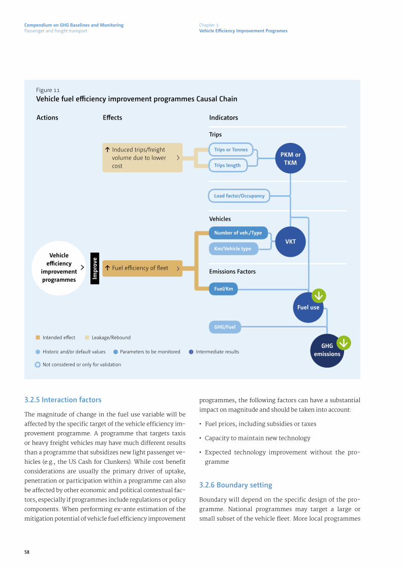
Compendium on GHG Baselines and MonitoringPassenger and freight transport
58
3.2.5 Interaction factors
The magnitude of change in the fuel use variable will be
affected by the specific target of the vehicle efficiency im-
provement programme. A programme that targets taxis
or heavy freight vehicles may have much different results
than a programme that subsidizes new light passenger ve-
hicles (e.g., the US Cash for Clunkers). While cost benefit
considerations are usually the primary driver of uptake,
penetration or participation within a programme can also
be affected by other economic and political contextual fac-
tors, especially if programmes include regulations or policy
components. When performing ex-ante estimation of the
mitigation potential of vehicle fuel efficiency improvement
programmes, the following factors can have a substantial
impact on magnitude and should be taken into account:
· Fuel prices, including subsidies or taxes
· Capacity to maintain new technology
· Expected technology improvement without the pro-
gramme
3.2.6 Boundary setting
Boundary will depend on the specific design of the pro-
gramme. National programmes may target a large or
small subset of the vehicle fleet. More local programmes
Figure 11
Vehicle fuel efficiency improvement programmes Causal Chain
Actions Effects Indicators
↑ Induced trips/freight volume due to lower cost
↑ Fuel efficiency of fleet
Trips
Vehicles
Emissions Factors
Impr
ove
PKM or TKM
Trips or Tonnes
Km/Vehicle typeVKT
GHG emissions
Fuel use
Intended effect Leakage/Rebound
Historic and/or default values Intermediate resultsParameters to be monitored
Fuel/Km
GHG/Fuel
Vehicle efficiency
improvement programmes
Number of veh./Type
Trips length
Load factor/Occupancy
Not considered or only for validation
Chapter 3Vehicle Efficiency Improvement Programes

Compendium on GHG Baselines and MonitoringPassenger and freight transport
59
may target a local subset. Upstream emissions should be
included for electric vehicles.
3.2.7 Key methodological issues
The GHG impact depends upon the number of vehicles
that adopt the new, fuel efficient changes and the amount
of fuel each vehicle can save thereby. Disaggregated data
for variables pertaining to VKT and fuel economy for di-
fferent types of vehicles may be needed if direct measu-
rement of fuel use is not possible. Specific methodologies
focus on variables that are key to the measure, for exam-
ple scrapping measures require knowledge of the age of
scrapped vehicles and tire replacement measures require
the range the range of specific rolling resistance of tires
within the fleet. A list of general issues to consider when
selecting a methodology includes:
· How much will new technology improve vehicle fuel
economy compared to existing fleet? Compared to Bu-
siness-As-Usual future projections?
· Allowing for fleet turnover, how will the benefits of these
improvements be realized over time in the on-road fleet?
· What unintended consequences (i.e., rebound effects)
might the policy have that could reduce its benefits,
e.g., people keep older vehicles longer, import more
used vehicles, or drive more because vehicle operating
costs are less?
1.2.8 Double counting concerns
Other policies and actions taken to mitigate GHG may
have synergistic or interaction effects on fuel efficiency
of vehicle fleets. Mitigation actions that affect the cost of
Table 19
Dimensions of boundary setting for vehicle fuel efficiency improvement programmes
Dimension Options for boundary setting
Geographical
Temporal
Upstream/downstream
Transport sub-sector
Emissions gasses
National, regional
Average life of vehicle, ~10-15 years
Upstream emissions for electric vehicles or other alternative fuels and upstream emissions of
baseline vehicles. Emissions from production of new vehicles.
Passenger, freight, specific type or use of vehicle (e.g., taxi, privately or publicly owned fleets)
CO2, CH4
Table 20
Actions with potential for double counting for mass transit investment mitigation actions
Mitigation action May affect this variable
National fuel economy standard
Fuel subsidies or tariffs
Vehicle import fees or rebates
Logistics measures
Fuel/km
Fuel/km
Fuel/km
Fuel/tonne-km
Chapter 3Vehicle Efficiency Improvement Programes

Compendium on GHG Baselines and MonitoringPassenger and freight transport
60
fuel or of certain classes of vehicles can distort the vehi-
cle market. This can lead to difficulty in attributing the
reduction to a particular action or to counting the same
tonnes more than once for different actions. In some
cases a dynamic baseline (or a technology improvement
factor) could account for the additional effects on fuel ef-
ficiency. Care should be taken in this regard if any of the
following policies or actions is being implemented con-
currently with fuel efficiency improvement programmes:
3.3 DETERMINING THE BASELINE AND CALCULATING EMISSION REDUCTIONS
3.3.1 Analysis approach
The baseline scenario for fuel efficiency improvement
programmes can be described as the overall fuel use by
the targeted vehicles in the existing fleet. Baseline emis-
sions are estimated by determining the total fuel use of
each type of vehicle within the boundary or by determin-
ing the vehicle kilometres travelled (VKT) by each vehicle
type and applying an appropriate emission factor.
Current fuel use or travel and fuel economy data serves
as the basis for this baseline calculation, which must be
projected into the future for ex-ante analysis and “coun-
terfactually projected” to create a BAU for ex-post anal-
ysis. Ex-ante analysis also requires a future projection of
the mitigation action scenario to compare to the baseline
scenario.
There are three general approaches for projecting or
counterfactually projecting fuel use and travel activity for
the baseline or fuel efficiency improvement programme
scenarios. In some cases one approach may be used for
baseline and another for mitigation scenario.
· Expert judgment based on historical trends, using time
series data gathered ideally for at least 10 years – can be
used for ex-ante projection or ex-post counterfactual
projection situations. Should be combined with a model
of fleet fuel economy characteristics.
· Fleet turnover models that estimate the number of
each type of vehicle by year.
· Economic projections and elasticity models that project
technology uptake based on costs and benefits. No me-
thodologies of this type were evaluated for this report.
Ex-post analysis also requires estimates of current miti-
gation scenario emissions, which are calculated, based on
the measured fuel use, or an activity measure such as VKT
or tonne/km is multiplied by the respective emission fac-
tors, within the defined boundaries of the project. (One
CDM methodology, for anti-idle devices, directly tracks
the amount of time the device is in use, leading to a direct
estimate of fuel saved.) Emission reductions, as always,
are the difference between the project emissions (real
or estimated ex-ante) and the baseline. Consideration of
upstream emissions from electricity production is usua-
lly included in methodologies involving electric power.
3.3.2 Uncertainties and sensitivity analysis
The most uncertain variable in the emission reduction
analysis of vehicle fuel efficiency improvement projects
is usually the ex-ante estimate of the uptake of the new
technology. There are also often uncertainties in the cur-
rent makeup of the fleet; leading to the use of average
values. Generally VKT or tonne/kilometres is assumed to
follow historic trends under baseline and mitigation sce-
narios, although some methodologies address rebound
effects or directly track VKT.
Ex-post methodologies also have characteristic uncer-
tainties related to the amount of change attributable to
the project itself. For example driver training or digital
efficiency monitoring devices can have uneven effects
depending on the driver. Also new technologies can result
in the driver more closely monitoring fuel efficiency in
the beginning until becoming accustomed to the change.
Chapter 3Vehicle Efficiency Improvement Programes

Compendium on GHG Baselines and MonitoringPassenger and freight transport
61
Box 3
MRV of mobile air conditioning and transport refrigeration mitigation actions
Many light and heavy duty vehicles have Refrigeration and/or Air Conditioning (RAC) systems. GHG emissions attributed
to these systems can be considered as direct or indirect. Direct emissions result from the release of high Global Warming
Potential (GWP) gas refrigerants such as hydro fluorocarbons (HFC) from these cooling systems. For example, HFC-134a,
one of the most common refrigerants (used i.a. in mobile air conditioning), has a GWP of 1,430 and HFC-404A, commonly
used in large refrigerated trucks, has a GWP of 3,922. Under the 2016 Kigali agreement, 197 countries committed to cut the
production and consumption of HFCs by more than 80 percent over the next 30 years1. Indirect emissions from vehicle RAC
mainly result from the energy consumption needed to power these systems, which increases the overall energy consumption
of the vehicle. While motor vehicle systems make up a small percentage of RAC emissions, it is important to be able to
estimate the GHG contribution and the potential reductions from transport sector mitigation actions.
Initial emissions occur during the production and charging process as HFC are produced and individual vehicle RAC systems
are charged with refrigerant (initial charge). After charging the vehicle system holds the HFC. The total amount of refrigerant
in the vehicle fleet at any given time is called the stock. Annual leakage rates of refrigerant in transport refrigeration are
high compared to other cooling applications because of the constant strain on system parts on the roads. Furthermore the
remaining refrigerant charge might be released during equipment or vehicle scrapping, etc., leading to additional emissions.
Structure of mitigation effects:
Direct emission reduction mitigation actions promote technologies that replace the conventional refrigerant, which will
typically have high GWP, with low-GWP or zero-GWP refrigerants, such as natural refrigerants like carbon dioxide (CO2)
or propane (HC-290) or unsaturated HFCs (e.g. HFO-1234yf). Indirect emission reduction mitigation actions, on the other
hand, focus on improving the energy efficiency of the refrigeration systems. This includes promoting adequately insulated
refrigerated vehicles as determined by the k-factor values of the international ATP agreement2. During operation, proper
servicing and refrigerant re-charging practices help to reduce leakages and thereby further reduce the climate impact. At the
end-of-life of the mobile AC or the car itself, the refrigerant can be evacuated and stored for recycling or destruction.
Determining the baseline and calculating reductions:
A top-down bulk based methodology can be developed by recording imported, produced and exported bulk HFC and
applying an emission factor. This can serve as a first step to indicate the potential for direct emissions or emission reductions.
However, indirect emission reductions cannot be estimated this way.
GIZ has developed a generalized bottom-up methodology based on a unit-stock model for the RAC sector that can be
applied to mobile systems. First the total stock of the RAC systems being considered is estimated. In the case of mobile or
transport cooling this would be held in the fleet of vehicles (or refrigerated trucks) that use air conditioning or refrigerating
systems. Then the direct and indirect emissions (BAU scenario) and potential emission reductions (mitigation scenario) of a
standardized unit of stock are estimated using the key variables below, which should be disaggregated, e.g. by technology,
refrigerant and other characteristics as needed to capture differences between scenarios:
· Initial charge (kg) and the dominant refrigerant that is used in the system
· Manufacture emission factor (%)
· In-use emission factor (%)
Continues on the next page
Chapter 3Vehicle Efficiency Improvement Programes

Compendium on GHG Baselines and MonitoringPassenger and freight transport
62
· Disposal emission factor (%)
· Product lifetime
· Average cooling capacity (kW)
· Average coefficient of performance (COP) – the amount of cooling provided per energy used
· Cost per unit
· Expected future annual growth rates – uptake of new technology
· Runtime ratios of the systems (similar to average annual runtime hours)
· Emission factor for electricity and fuels to run system
Mitigated emissions are then calculated as the difference between the BAU scenario and the mitigation scenario as in other
methodologies.
For more information please consult the following modules of the technical handbook NAMAs in the refrigeration, air
conditioning and foam sectors (sub sectors mobile air conditioning and transport refrigeration):
Module 1 Inventory: https://www.giz.de/expertise/downloads/giz2014-en-NAMA-Handbook-Module-1_WEB.pdf
Module 5 Mitigation Scenarios: https://www.giz.de/expertise/downloads/giz2014-en-NAMA-Handbook-Module-5_WEB.pdf
Module 7 Measurement, Reporting, Verification: https://www.giz.de/expertise/downloads/giz2014-en-NAMA-Handbook-
Module-7_WEB.pdf
1 <https://www.epa.gov/ozone-layer-protection/recent-international-developments-under-montreal-protocol>2 The Agreement on the international carriage of Perishable Foodstuffs and on the Special Equipment to be used for such Carriage (French and
international abbreviation: ATP), see <http://www.unece.org/trans/main/wp11/atp.html>3 Go to <https://www.giz.de/expertise/html/4809.html> and find “NAMAs in the refrigeration, air conditioning and foam sectors”, then click on
“more” to see all volumes of the technical handbook.
Chapter 3Vehicle Efficiency Improvement Programes
Figure 12
Causal Chain of emissions from RAC
Stock (=vehicles in use) → Bank
Disposal Emissions Energy Consumption
Production of vehicles (first fill)
Manufacture Emissions
Refill Indirect EmissionsDirect Emissions
Total EmissionsDemand
Fill
Service Emissions (Refill)
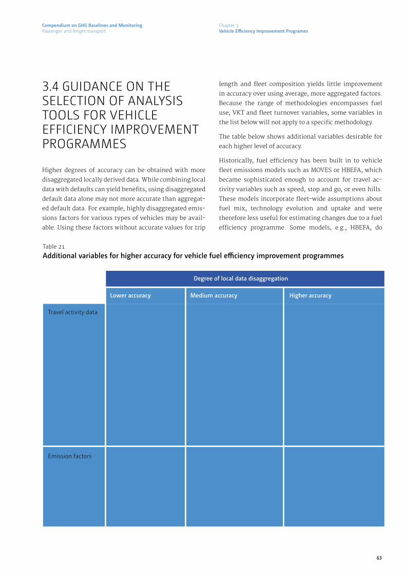
Compendium on GHG Baselines and MonitoringPassenger and freight transport
63
3.4 GUIDANCE ON THE SELECTION OF ANALYSIS TOOLS FOR VEHICLE EFFICIENCY IMPROVEMENT PROGRAMMES
Higher degrees of accuracy can be obtained with more
disaggregated locally derived data. While combining local
data with defaults can yield benefits, using disaggregated
default data alone may not more accurate than aggregat-
ed default data. For example, highly disaggregated emis-
sions factors for various types of vehicles may be avail-
able. Using these factors without accurate values for trip
length and fleet composition yields little improvement
in accuracy over using average, more aggregated factors.
Because the range of methodologies encompasses fuel
use, VKT and fleet turnover variables, some variables in
the list below will not apply to a specific methodology.
The table below shows additional variables desirable for
each higher level of accuracy.
Historically, fuel efficiency has been built in to vehicle
fleet emissions models such as MOVES or HBEFA, which
became sophisticated enough to account for travel ac-
tivity variables such as speed, stop and go, or even hills.
These models incorporate fleet-wide assumptions about
fuel mix, technology evolution and uptake and were
therefore less useful for estimating changes due to a fuel
efficiency programme. Some models, e.g., HBEFA, do
Table 21
Additional variables for higher accuracy for vehicle fuel efficiency improvement programmes
Lower accuracy Medium accuracy
Degree of local data disaggregation
Higher accuracy
Travel activity data
Emission factors
• Overall fuel use by vehicle
type
• Or:
• Total vehicle stock (by type)
• Total VKT by vehicle type
(base year)
• Total VKT by vehicle type
(future-year projections)
• Expected incremental
change in cost of new
vehicle (by type)
• Average fuel economy of
on-road vehicle fleet (by
vehicle type)
• Future-year projections of
new vehicle efficiency by
vehicle type
• Future-year projections of new
vehicle sales (by vehicle type)
• Scrappage/turnover rates or age
distribution by vehicle type
• Observed, sales-weighted new
vehicle efficiency by vehicle type
• Observed increase in cost of new
vehicle (by type)
• Observed increase in volume of
imported used vehicles
• Current and recent historical
efficiency (test cycle) of new vehicles,
by vehicle type to be regulated
• Adjustment for actual on-road
efficiency/emissions versus test
cycle/certification efficiency
• Future-year projections of new
vehicle efficiency (baseline)
• Mileage accumulation rates by vehicle
type
• “Rebound effect” – Percent increase in
VKT due to decreased cost/km
• Price of fuel (for rebound effect)
• “Purchase effect” – Expected shift
in consumer purchases by vehicle
efficiency or type in response to price
differential
• “Turnover effect” – Expected slower
rate of fleet turnover due to higher
new vehicle cost
• “Import effect” – Expected increase in
used imported vehicles due to higher
new vehicle cost
• Observed, sales-weighted new vehicle
efficiency by vehicle type
Chapter 3Vehicle Efficiency Improvement Programes

Compendium on GHG Baselines and MonitoringPassenger and freight transport
64
have a version which allows different fleets to be simu-
lated. The sketch planning tool EERPAT allows modifica-
tion to its fuel efficiency defaults while maintaining the
link with VKT inputs.
Some methodologies that were developed for CDM or
NAMAs focus guidance to measure the changes from a
programme or project promoting a single technology.
Other methodologies offer a wider scope of application.
Figure 13
Navigating classes of available methods and associated tools for vehicle fuel efficiency improvement programmes
Prioritize policies
Objective
Report results
Mitigation planning
Emissions trading
Ex-a
nte
Lower accuracy Medium accuracy Higher accuracy
Ex-p
ost
Spreadsheet or software tool Guidance document
Spreadsheet tools with defaults CCAP Emissions
Guidebook EERPAT
Spreadsheet tools with local data
CDM methodologies
Other bottom-up methodologies/
guidance
MRV-Blueprint Road Freight Transport NAMA in Mexico
Travel models
MRV-Blueprint: Low rolling resistance tyre labelling and phase out schemes
UNDP E-BRT – Sri Lanka: NAMA on eBRT Systems of Colombo
AMS-III.AP.*
AMS-III.AA.*
AMS-III.AT.*
AMS-III.BC.*
AMS-III.C.*
AMS-III.S.*
(*) AMS-III.AP.: Transport energy efficiency activities using post-fit idling stop device, AMS-III.AA.: Transportation energy efficiency activities using retrofit technologies, AMS-III.AT.: Transportation energy efficiency activities installing digital tachograph systems to commercial freight transport fleets, AMS-III.BC.: Emission reductions through improved efficiency of vehicle fleets, AMS-III.C.: Emission reductions by electric and hybrid vehicles, AMS-III.S.: Introduction of low-emission vehicles/technologies to commercial vehicle fleets
Chapter 3Vehicle Efficiency Improvement Programes

Compendium on GHG Baselines and MonitoringPassenger and freight transport
65
As NAMAs and broader transport programmes spread,
some spreadsheet methodologies were developed that
incorporated assumptions about uptake of technologies,
or allowed user inputs. Sri-Lanka developed a simplified
CDM-style methodology for GHG as part of an overall
project which also used the UNDP Sustainable Develop-
ment Evaluation Tool.
Figure 13 maps existing methodologies and tools for mass
transit investments according to their purpose (y axis)
and level of accuracy (x axis).
3.4.1 Description of tool types
The following sections describe a number of tools that
are available for estimating GHG reduction from fuel effi-
ciency improvement mitigation actions. They are classi-
fied according to similarities in methodology.
3.4.2 Disaggregate emissions models
The EERPAT tool is a non-spatial policy analysis tool, de-
signed to provide rapid analysis of scenarios that com-
bine effects of various policy and transportation system
changes. In order to provide quick response comparing
many scenarios, it makes a number of simplifying as-
sumptions (consistent with emissions and advanced re-
gional travel demand modelling practice) that somewhat
limit the detail and precision of its outputs compared to a
properly set up MOVES or similar implementation. It can
be modified to accept alternative fuel usage or efficiency
inputs if uptake levels are known and apply them to VKT
data specific to a region.
3.4.3 Disaggregated bottom-up ex-post guidance
These are CDM methodology documents or other MRV
guidance documents that detail the disaggregated var-
iables that should be collected. The documents focus on
delineating a specific type of mitigation actions and often
give precise methodologies on how to collect the appropri-
ate variables to calculate emissions reductions for them.
CDM tools are primarily used ex-post; ex-ante guidance is
only found for additionality testing, which states that fu-
ture trip length and mode share must be estimated outside
of the methodology. Defaults are not usually included al-
though default sources may be referenced. Some guidance
documents associated with specific projects may have
spreadsheets prepared for the case study.
Because there are many approaches to improving fuel
economy of vehicles that lend themselves to CDM or
NAMA designs, a number of methodologies have been de-
veloped. They differ mainly in the boundaries, e.g., transit
or truck, public or commercial fleets, etc., and in the spe-
cific measure being monitored. The general framework
Chapter 3Vehicle Efficiency Improvement Programes
Table 22
Disaggregate emissions models for vehicle fuel efficiency improvement programmesEase of use/data collection: Highly resource and data intensive
Name Application /summary
Scope Computer based
Methodology documentation
Defaults Provided
Data collection guidance
Cost of tool
EERPAT Includes
emissions
module
Very good Complete
defaults for USA
– allows user
input for other
areas
Non-spatial
disaggregate
model
Yes Good Free

Compendium on GHG Baselines and MonitoringPassenger and freight transport
66
has even been extended to a methodology for improving
fuel efficiency of large ships. Generally methodologies
try to track the number of vehicles affected (or the VKT of
affected vehicles) and the fuel efficiency gain per vehicle
from the change, some also offer guidance on measuring
fuel use directly if the fleet size or ownership allows.
3.4.5 Simple Bottom-up tools with mostly default data
This spreadsheet program accepts limited local data but
offers default values for emissions. VKT estimates or actu-
al fuel use must be entered by the user.
Name Application /summary
Scope Computer based
Methodology documentation
Defaults Provided
Data collection guidance
Cost of tool
MRV-Blueprint Road Freight Transport NAMA in Mexico
Improvement of Fuel Efficiency for Taxies in Vietnam”
Reducing vessel emissions through use of advanced hull coatings
AMS-III.AP.: Transport energy efficiency activities using post-fit idling stop device
Modernization of
heavy duty truck
fleet (national
level)
Vehicle fuel effi-
ciency measures
Transit efficiency
measures (higher
occupancy rate/
lower non-pas-
senger mileage)
Retrofitting
large freight or
passenger ships
Public transit fleets
Very Good
Very Good
Excellent
Very Good
Yes, for Mexican
fleet
None
None
None
Modernization
program
(scrapping and
finance)
Improving fuel
efficiency for taxis
Ship fuel efficiency
improvement
Devices to stop
idling when
vehicle not
moving
Spreadsheet
available
No
No
No
Very Good
Very Good
Very Good
Very Good
Free
Free
Free
Free
Continues on the next page
Chapter 3Vehicle Efficiency Improvement Programes
Table 23
Disaggregated bottom-up ex-post guidance for vehicle fuel efficiency improvement programmesEase of use/data collection – moderately resource and data intensive
MRV-Blueprint: Low rolling resistance tyre labelling and phase out schemes
Tire-labelling
and phase- out
for heavy-duty
trucks w/ GVW
>3.5 tonnes
(national level)
Very Good Yes, for EU fleetFitting trucks
with lower
rolling resistance
tires
No Fair Free

Compendium on GHG Baselines and MonitoringPassenger and freight transport
67
AMS-III.AA.: Transportation energy efficien-cy activities using retrofit technologies
AMS-III.AT.: Transportation energy efficien-cy activities installing digi-tal tachograph systems to commercial freight trans-port fleets
Commercial
passenger
transport
Centrally owned
freight or
passenger fleets
Very Good
Very Good
None
None
Engine retrofit
(replacement) with
more efficient engine
Installing vehicle or
engine tracking and
recording systems
No
No
Very Good
Excellent
Free
Free
Name Application /summary
Scope Computer based
Methodology documentation
Defaults Provided
Data collection guidance
Cost of tool
AMS-III.C.: Emission reduc-tions by electric and hybrid vehicles
AMS-III.S.: Introduction of low-emission vehicles/technologies to commercial vehicle fleets
UNDP E-BRT – Sri Lanka: NAMA on eBRT Systems of Colombo
Passenger
and freight
transportation
Includes lower
emissions by
means of electric
or hybrid
Developed
specifically for
Sri Lanka project,
could be adapted
for other measures
changing fuel
efficiency
Very Good
Good
Very Good
None
None
Yes, values based
on local study/
manufacturer
data/ national
or international
averages
New electric and/or
hybrid vehicles that
displace the use of fossil
fuel vehicles
Introduce vehicles with
lower emissions per
kilometre
Substitution of electric
buses for diesel in BRT
system
No
No
No
Very Good
Fair
Very Good
Free
Free
Free
AMS-III.BC.: Emission reduc-tions through improved efficiency of vehicle fleets
Centrally owned
freight or
passenger fleets
Very Good NoneInstalling one or more:
(a) Idling stop device;
(b) Eco-drive systems;
(c) Tire-rolling resistance
improvements;
(d) Air-conditioning sys-
tem improvements;
(e) Use of low viscosity oils
(f) Aerodynamic drag
reduction measures
(g) Transmission improve-
ments
(h) Retrofits that improve
engine efficiency
No Fair Free
Chapter 3Vehicle Efficiency Improvement Programes

Compendium on GHG Baselines and MonitoringPassenger and freight transport
68
Table 24
Simple bottom-up tools with mostly default data for vehicle fuel efficiency improvement programmesEase of use/data collection: Moderate to low
Name Application /summary
Scope Computer based
Methodology documentation
Defaults Provided
Data collection guidance
Cost of tool
CCAP Emissions Guidebook
Ex-ante tool;
sketch planning
estimates based
on combining
local data and
defaults;
Good Emission factors
for US fleet,
other factors can
be entered
Uptake rates
Fuel efficiency
incentives
Anti-idling
campaigns
Vehicle
scrappage
feebates
Yes Fair Free
Table 25
Minimum indicator set for mass transit mitigation action
Category Indicator Normal monitoring frequency
Implementation indicator
Performance indicators
Impact indicators
Construction and operation of new transit line
Ridership on new line
Traffic in corridor
Calculated passenger transport VKT by mode
Latest emission rates by mode
Calculated emissions in study area
One time or by construction phase
Annual
Annual
5 years
5 years
5 years
Chapter 3Vehicle Efficiency Improvement Programes
3.5 MONITORING
Performance of the mitigation action can be monitored
by tracking key variables over time. CDM methodologies
generally require annual monitoring. Fuel efficiency ef-
fectiveness of technologies should be measured at imple-
mentation and should in most cases remain unchanged.
Uptake of technologies should be monitored annually to
determine the penetration into the fleet. Measures that
apply technology to individual privately owned commer-
cial fleets can monitor penetration with cooperation from
the owners. Broader government programs will keep re-
cords of scrapped vehicles or subsidies that are issued.
Table 25 presents a minimum list of key variables and
recommended intervals for measurement if no other re-
quirements are present, (e.g., CDM).

Compendium on GHG Baselines and MonitoringPassenger and freight transport
69
3.6 EXAMPLE − MEXICAN FREIGHT NAMA
The Mexican Freight NAMA is a fuel efficiency mitigation
action which has as its centrepiece continuation of a pro-
gramme of scrapping of trucks older than 10 years and re-
placing them with trucks less than 6 years old. When this
is done it allows the owner to receive a subsidy of up to 25%
of the value of the new truck by the Mexican Fleet Modern-
ization Program. There are also credits for users to finance
newer fuel efficient trucks without scrapping an older one.
Under the existing programme an ex-post evaluation is
used by Secretaría de Comunicaciones y Transportes and
Instituto Nacional de Ecología y Cambio Climático to esti-
mate the real GHG-emission mitigation. Essentially, the
calculation compares emissions of the scrapped truck,
which represents the baseline, to the emissions of the
replacement truck (based on the fuel efficiency and total
kilometres travelled with the truck).
For ex-ante analysis the NAMA developed an MRV system
that refines the old method to include a direct effect and
an indirect effect (due to new trucks being used more than
old). They also incorporated a fleet survival rate tool. Using
these tools they calculated that combining scrapping and
credits for newer trucks would give a higher reduction po-
tential than either program alone.
Further details are available at:
http://transport-namas.org/wp-content/uploads/2014/10/
TRANSfer_MRV-Blueprint_Truck_Scrapping_MX_draft.pdf
Chapter 3Vehicle Efficiency Improvement Programes

Compendium on GHG Baselines and MonitoringPassenger and freight transport
70
Chapter 4
ALTERNATIVE FUELS INCENTIVES, REGULATION AND PRODUCTION

Compendium on GHG Baselines and MonitoringPassenger and freight transport
71
4.1 DESCRIPTION AND CHARACTERISTICS OF ALTERNATIVE FUELS INCENTIVES, REGULATION AND PRODUCTION MITIGATION ACTIONS
This mitigation action type covers a range of projects and
policies that displace liquid fossil fuels with liquid motor
fuels from renewable sources or with gaseous fossil fuels.
Measures that promote electric powered vehicles are in-
cluded in section 3, vehicle energy efficiency, because liq-
uid or gaseous fuels are used directly in vehicles and have
specific methodologies associated with their production.
This includes technologies, infrastructure, and regula-
tory strategies for promoting bio-diesel, other plant oils,
bio-CNG, as well as fossil CNG and LNG. These actions are
intended to reduce overall GHG emissions by increasing
use of less carbon intensive fuels and decreasing the use
of more carbon intensive fuels to provide the energy re-
quired for travel activity. The reduced carbon intensity of
the new fuels can be from reduced upstream emissions or
from lower inherent carbon intensity, or both.
The outcomes of successful implementation of this mit-
igation action are expected to reduce the overall GHG
emissions from a given amount of travel activity, when
taking into account upstream and direct emissions.
Alternative fuels mitigation actions can create economic
benefits in areas of production. There is also the poten-
tial for reduction of various toxic pollutants. However, if
not properly designed alternative fuel mitigation projects
could result in negative impacts on land use, food produc-
tion or even displacement of persons. In fact, first gener-
ation biofuels have been found in some cases to actual-
ly be more emission intensive than conventional fuels if
properly accounted. As a result, In the European Union the
GHG-savings from biofuels have to be at least 50 % to be
eligible for support schemes (according to the Renewable
Energy Directive).
4.2 STRUCTURE OF MITIGATION EFFECTS
4.2.1 Cause-impact chain
Alternative fuels mitigation actions should result in
measurable effects that are reflected in three key indica-
tors in bottom-up models (ASIF approach). The expected
changes in those variables will cause the desired out-
comes. See Figure 14.
4.2.2 Key variables to be monitored
The key variables that are expected to change by alterna-
tive fuels mitigation actions are listed below, followed by
the expected mechanism that causes them to change.
4.2.3 Monitor for intended effects
· Number of vehicles by fuel type
· Fuel use – amount of fuel used, disaggregated by type of
fuel, is the key indicator for this type of action because
the amounts of the various types of fuels that are used
will change. In some cases this will be measured di-
rectly and in other cases based on VKT of vehicles that
use alternative fuels and relative fuel consumption of
vehicle types.
· GHG/fuel – the GHG intensity per caloric output of each
type of fuel must be determined.
· GHG/fuel – upstream emission from the production of
fuel, charging infrastructure, etc., can vary greatly de-
pending upon the process and type of fuel. This must be
included in the overall GHG intensity.
Chapter 4Alternative fuels incentives, regulation and production

Compendium on GHG Baselines and MonitoringPassenger and freight transport
72
4.2.4 Interaction factors
The magnitude of change in the key variable of fuel use
will be affected by the specific characteristics of the al-
ternative fuels mitigation action. The economic and po-
litical context into which the alternative fuels are intro-
duced is very important for actions in which uptake is
determined mainly by the market as affected by incenti-
ves or taxes. In addition some strategies impose quotas or
portfolio standards for renewable or alternative fuels. For
this reason the following factors need to be considered
when performing ex-ante estimation of the mitigation
potential of alternative fuels mitigation actions, if they
are not part of the action itself.
· Incentive is designed to account for full fuel-cycle GHG
emissions
Figure 14
Alternative fuels incentives Causal Chain
Actions Effects Indicators
Promote alternative fuels (e.g.
biofuel quota, electrification)
↑ Vehicles using alternative fuels
↓ Carbon content of fuel / GHG intensity
↑ Quantity of alternative fuel
↓ Quantity of liquid fossil fuel
↑ Upstream emissions from fuel production
Trips
Vehicles
Emissions
Fuel
PKM
Load factor/Occupancy
Number of veh./Type
Persons
Trips/Person
Km/Trip
Trips/Mode
Km/Vehicle type
GHG emissionsHistoric and/or default values Intermediate resultsParameters to be monitored
Fuel/Km
GHG/Fuel
Not considered or only for validation
Intended effect Life cycle effect
VKT
Fuel use
Chapter 4Alternative fuels incentives, regulation and production

Compendium on GHG Baselines and MonitoringPassenger and freight transport
73
· Similar low-carbon standards/ incentives adopted or
proposed in neighbouring countries
· Expected ability of fuel suppliers to produce and distri-
bute low-carbon/GHG fuels
· Expected ability of vehicle manufacturers to produce
dedicated or bi-fuel vehicles
4.2.5 Boundary setting
The boundary will depend on the type of mitigation action.
Fuel production projects usually include the production
area and the transportation use area. Vehicle conversion
projects are more often limited to the use area, with ups-
tream emissions incorporated into the emissions factor.
Upstream balance of emissions/sinks are important to in-
clude for the production of bio-fuels, as sinks contribute
to the mitigation effect, other emissions such as metha-
ne leakage of LNG production may or may not be included
depending upon the methodology. If this is done upstream
emissions also have to be considered for the baseline fuels.
In the CDM methodologies the temporal boundary of a
vehicle conversion projects is limited to the lifetime of
the original fleet. Bio-fuel production can extend to the
life of the project.
4.2.6 Key methodological issues
The GHG impact depends upon the reduced GHG inten-
sity of the alternative fuels vs conventional fuels as well
as the total amount of each fuel that is used to support
transportation activity. Ex-ante prediction of the amount
of fuels used is a difficulty for all methodologies. Calcula-
ting the upstream emissions can also be complicated and
data intensive. Tracking the current fuel use is a straigh-
tforward challenge.
A list of specific issues to consider when selecting a me-
thodology include:
· Is fuel use measured at the distribution point or the end
user?
· What level of ex-ante estimation is needed?
· How effective will the action be at encouraging consu-
mers to switch to different types of fuels?
· What are the full life-cycle GHG impacts of the alterna-
tive fuels for which incentives are provided?
4.2.7 Double counting concerns
Other policies and actions taken to mitigate GHG may
have synergistic or interaction effects on the amount and
type of fuel used or the makeup of the vehicle fleet.
This can lead to difficulty in attributing the reduction to
a particular action or to counting the same tonnes more
than once for different actions. Care should be taken in
this regard if any of the following policies or actions is
being implemented concurrently. In some cases a dy-
Table 26
Dimensions of boundary setting for alternative fuels mitigation actions
Dimension Options for boundary setting
Geographical
Temporal
Upstream/downstream
Transport sub-sector
Emissions gasses
National, regional, local
5 – 10, over 20 years for production projects
Production process emissions for harvesting, refining, etc.; methane leakage
Specific commercial or transit fleets, all vehicles capable of conversion or replacement
CO2, CH4, N2O (from production)
Chapter 4Alternative fuels incentives, regulation and production

Compendium on GHG Baselines and MonitoringPassenger and freight transport
74
Table 27
Actions with potential for double counting for alternative fuels mitigation actions
Mitigation action May affect this variable
Fuel economy standards
Fuel subsidy removal
Fuel efficiency incentives
Vehicle scrapping schemes
Taxes and tariffs on fossil fuels
Amount of fuel used by type
Amount of fuel used by typeFuel/km
Amount of fuel used by type
Number of conventional vehicles
Amount of fuel used by type
namic baseline can account for the effect without the al-
ternative fuel incentive; in other cases it may be better
to analyse the combined effect of the actions rather than
trying to allocate the reductions among the various mit-
igation actions.
4.3 DETERMINING THE BASELINE AND CALCULATING EMISSION REDUCTIONS
4.3.1 Analysis approach
Alternative fuel mitigation actions are analysed by de-
termining the amount of conventional fuel that is or will
be displaced by the alternative fuel. The respective emis-
sions of the amount of conventional fuel and the amount
of alternative fuels are calculated and the difference is
the reduction attributed to the action. Two general ap-
proaches are used
1. Top-down, mostly ex-post, based on directly measu-
ring the amount of alternative fuel that is used (typically
from fuel sales data), and assuming it displaced the same
calorific equivalent of fossil fuel and corrected for vehi-
cle efficiency changes due to fuel change, if applicable.
2. Bottom-up, mostly ex-ante, based on the distance tra-
velled (used mainly for new vehicles projects or vehicle
replacement projects). Bottom-up methods usually as-
sume the same distance under baseline and mitigation
scenarios and correct for variation in caloric content
of fuels and for vehicle efficiency changes due to fuel
change, if applicable. Also used for ex-post for vehicle
replacement projects that only cover a specific subset
of vehicles, e.g., a taxi fleet, but don’t have a large effect
on fuel sales overall.
The baseline scenario for alternative fuel mitigation ac-
tions can be described as the mix of fuels that is currently
in place or expected to occur under baseline policies. Cur-
rent fuel sales data serves as the basis for this baseline
calculation, which must then be projected into the future
for ex-ante analysis and “back cast” for ex-post analysis.
There are two general approaches for projecting or coun-
terfactually projecting travel activity for baselines or al-
ternative fuel mitigation action scenarios:
· Expert judgment based on historical trends, using time
series data gathered ideally for at least 10 years – can
be used for ex-ante projection or ex-post counterfac-
tual projection situations. Should be combined with
knowledge of fleet characteristics.
· Economic projections and elasticity models. No metho-
dologies of this type were evaluated for this report.
Consideration of upstream emissions from fuel produc-
tion varies between methodologies, depending on the
type of fuel project that is being considered.
Chapter 4Alternative fuels incentives, regulation and production

Compendium on GHG Baselines and MonitoringPassenger and freight transport
75
4.3.2 Uncertainties and sensitivity analysis
The first uncertainty in the emission reduction analysis
of alternative fuel mitigation actions is usually the ex-an-
te estimate of the amount of fossil fuels that will be dis-
placed by new supplies of alternative fuel from a mitiga-
tion action. In mitigation actions where a known number
of vehicles are replaced, or new vehicles are introduced
this problem is less critical. It is also important to have
a clear understanding of the availability, annual volume
outputs, of alternative fuels for these types of actions.
The other important uncertainty is estimating the
life-cycle emissions for alternative fuels. Bio-fuels can be
cultivated and produced by different methods that result
in a range of life-cycle emissions. Proper analysis of feed-
stock production and transport as well as fuel production
and distribution are crucial to determining the actual re-
ductions of an action. Some widely accepted methods are
available. Sustainability criteria according to Renewable
Energy Directive (2009/28) and International standard on
sustainability criteria for bio energy (ISO13065) are two
examples. There are also a number of voluntary schemes
that certify sustainability criteria on biofuels7.
For conversion to CNG it is important to look at well-to-
wheel emissions as a minimum. CNG conversions may
come with CNG leakage and reduced catalytic activity for
already old fleets. A 2% CNG leakage, which is within the
range of potential performance of CNG conversions, can
immediately negate the GHG benefits compared to gaso-
line. On the other hand, brand new vehicles with properly
calibrated engines and systems designed to reduce leak-
age may produce the expected GHG reductions.
6 See https://ec.europa.eu/energy/en/topics/renewable-energy/biofuels/voluntary-schemes
Table 28
Additional variables for higher accuracy for vehicle fuel efficiency improvement programmes
Lower accuracy Medium accuracy
Degree of local data disaggregation and context variables
Higher accuracy
Fuel sales data
Emission factors
Vehicle and
infrastructure data
• Current volume of
transportation fuels
sold in country, by
fuel type
• Forecast-year
volume of
transportation fuels
sold in country, by
fuel type
• Default emission
factors for fuel types
• Current volume
• Forecast- year volume
• Projected fuel cost differential versus
conventional fuel after incentive,
and net change in vehicle operating
cost for consumer
• Life-cycle emissions associated with
unit of fuel, by type
• Fraction of existing vehicle fleet
capable of using alternative fuel(s)
targeted by policy
• Extent to which renewable/low-GHG
fuel infrastructure is deployed and
fuel available
• Current volume
• Forecast- year volume
• Total volume of fuels sold within broader re-
gion, by fuel type (to examine diversion effects)
• Analysis of whether alternative fuel demand
would be new, or diverted from other
existing uses
• Maximum value of available alternative fuels
• Actual life-cycle emissions considering
production pathways used
• Projected change in vehicle purchase price
(for dedicated-fuel vehicles) and payback
period given projected fuel prices
• Differences in key performance attributes
for alternative fuel versus conventional fuel
vehicles (e.g., range, cargo capacity, safety)
Chapter 4Alternative fuels incentives, regulation and production

Compendium on GHG Baselines and MonitoringPassenger and freight transport
76
4.4 DETERMINING THE BASELINE AND CALCULATING EMISSION REDUCTIONS
Higher degrees of accuracy can be obtained with more
disaggregated data, if some or all of the data is locally de-
rived. While combining local data with defaults can yield
benefits, using disaggregated default data alone is seldom
more accurate than aggregated default data. Estimating
the penetration of alternative fuels can also require con-
textual data about the fleet and fuel infrastructure.
Evaluation methodologies for mitigation actions promot-
ing alternative fuels have been developed under the CDM
for several types of actions. Each methodology is fairly
specific and limited in scope of application. Aside from
Figure 15
Navigating classes of available methods and associated tools for alternative fuels mitigation actions
Prioritize policies
Objective
Report results
Mitigation planning
Emissions trading
Ex-a
nte
Lower accuracy Medium accuracy Higher accuracy
Ex-p
ost
Spreadsheet or software tool Guidance document
Spreadsheet tools with defaults CCAP Emissions
Guidebook EERPAT
MOVES
Spreadsheet tools with local data
AFLEET
CDM methodologies
Travel models
AMS-III.T.*
AMS-III.AK.*
AMS-III.AQ.*
AMS-III.AY.*
AMS-III.S.*
ACM0017*
Chapter 4Alternative fuels incentives, regulation and production
(*) AMS-III.T.: Plant oil production and use for transport applications, AMS-III.AK.: Biodiesel production and use for transport applications, AMS-III.AQ.: Introduction of Bio-CNG in transportation applications, AMS-III.AY.: Introduction of LNG buses to existing and new bus routes, AMS-III.S.: Introduction of low-emission vehicles/technologies to commercial vehicle fleets, ACM0017: Production of biodiesel for use as fuel

Compendium on GHG Baselines and MonitoringPassenger and freight transport
77
CDM methodologies there exist some general tools that
can be used for evaluating the emissions of different fuel
mixes, given inputs of fuel use.
Figure 15 maps existing methodologies and tools for mass
transit investments according to their purpose (y axis)
and level of accuracy (x axis).
4.4.1 Description of tool types
The following sections describe a number of tools that are
available for estimating GHG reduction from alternative
fuels projects. They are classified according to similarities
in methodology.
4.4.2 Disaggregate emissions models
The US EPA supports the MOtor Vehicle Emission Simulator
(MOVES). This is a state-of-the-science emission modelling
system that estimates emissions for mobile sources at the
national, county, and project level for criteria air pollutants,
greenhouse gases, and air toxics. Although the defaults
included are for the United States fleet, given appropriate
data on VKT, fuel types and fleet makeup it can be modi-
fied to predict emissions in other regions. The 2015 version
will automatically adjust fuel property changes based on
user-made fuel property changes (e.g., ethanol), although
this requires the user to have reliable life cycle data.
The EERPAT tool is a non-spatial policy analysis tool, de-
signed to provide rapid analysis of many scenarios that
combine effects of various policy and transportation sys-
tem changes. In order to provide quick response comparing
many scenarios, it makes a number of simplifying assump-
tions (consistent with emissions and advanced regional
travel demand modelling practice) that somewhat limit the
detail and precision of its outputs compared to a properly
set up MOVES implementation. It can be modified to accept
input data specific to a region, including alternative fuel
usage estimates, and will calculate emissions.
The Alternative Fuel Life-Cycle Environmental and Eco-
nomic Transportation (AFLEET) Tool allows users to ex-
amine both the environmental and economic costs and
benefits of alternative fuel and advanced vehicles. It was
developed for stakeholders to estimate petroleum use,
greenhouse gas emissions, air pollutant emissions, and
cost of ownership of light-duty and heavy-duty vehicles
using simple spreadsheet inputs.
4.4.3 Disaggregated bottom-up ex-post guidance
These are CDM methodology documents that detail the
specific variables that should be collected. The docu-
Chapter 4Alternative fuels incentives, regulation and production
Table 29
Disaggregate emissions models for alternative fuels mitigation actionsEase of use/data collection: Highly resource and data intensive
Name Application /summary
Scope Computer based
Methodology documentation
Defaults Provided
Data collection guidance
Cost of tool
MOVES
EERPAT
AFLEET
Requires VKT
and speed
inputs
Includes
emissions
module
Fleeet data and
fuel costs
Very good
Very good
Good
Defaults for USA
– allows user
input for other
areas
Defaults for USA
– allows user
input for other
areas
Defaults for
USA including
WTW upstream
emissions
Emissions model
Non-spatial
disaggregate
model
Emissions and
costs model for
fleets
Yes
Yes
Yes
Fair
Good
Good
Free
Free
Free

Compendium on GHG Baselines and MonitoringPassenger and freight transport
78
ments give methodologies on how to collect these var-
iables and how to calculate emissions using them. Each
methodology is tailored to the specific type of fuel or
the specific type of fleet the fuel will be used in. Because
CDM is focused on documenting precise amounts of real
tonnes, CDM tools are primarily used ex-post. Method-
ologies that focus on production offer careful definitions
for conservatively estimating the actual amount of fuel
produced and incorporating upstream emissions. Meth-
odologies for vehicle-centred actions focus on calculating
emissions per passenger or tonne kilometre.
4.4.4 Simple bottom-up tools with mostly default data
This is a spreadsheet program that accepts limited local
data but offers default values for emissions based on US
experience. VKT estimates or actual fuel use must be en-
tered by the user.
4.5 MONITORING
Performance of the mitigation action is monitored by
tracking key variables over time. The monitoring frequen-
cy will vary, depending on the monitoring regimen and the
budget available for data collection. Measures that focus on
fuel production will have different monitoring challenges
from measures that focus on introducing alternative fuel
vehicles to the fleet. Production of alternative fuels will be
Table 30
Disaggregated bottom-up ex-post guidance for alternative fuels mitigation actionsEase of use/data collection: Moderately resource and data intensive (may require agricultural production data)
Name Application /summary
Scope Computer based
Methodology documentation
Defaults Provided
Data collection guidance
Cost of tool
AMS-III.T.: Plant oil production and use for transport applications
AMS-III.AK.: Bio-diesel production and use for trans-port applications
AMS-III.AQ.: Intro-duction of Bio-CNG in transportation applications
AMS-III.AY.: In-troduction of LNG buses to existing and new bus routes
ACM0017: Produc-tion of biodiesel for use as fuel
AMS-III.S.: Introduc-tion of low-emission vehicles/technolo-gies to commercial vehicle fleets
Cultivation, pro-
duction and use
for transport
Cultivation, pro-
duction and use
for transport
Cultivation, pro-
duction and use
Must replace
gasoline or
diesel existing or
planned vehicles
Cultivation, produc-
tion and use
Includes lower
emissions by
means of alter-
native fuels
Good
Good
Good
Very Good
Very Good
Good
None
None
None
None
None
None
Displacement of die-
sel with plant oils
Displacement of die-
sel with bio-diesel
Use of CNG from
biomass in transport
Introduction of new
LNG busses to exist-
ing or new routes
Production, sale
and consumption of
blended biodiesel
used as fuel
Introduce vehicles
with lower emis-
sions per kilometre
No
No
No
No
No
No
Fair
Fair
Fair
Very Good
Very Good
Fair
Free
Free
Free
Free
Free
Free
Chapter 4Alternative fuels incentives, regulation and production

Compendium on GHG Baselines and MonitoringPassenger and freight transport
79
Chapter 4Alternative fuels incentives, regulation and production
Table 31
Simple bottom-up tools with mostly default data for alternative fuels mitigation actionsEase of use/data collection: Moderate to low
Name Application /summary
Scope Computer based
Methodology documentation
Defaults Provided
Data collection guidance
Cost of tool
CCAP Emissions Guidebook
Ex-ante tool; sketch
planning estimates
based on combining
local data and defaults;
Good US emission
factors for
bio-diesel and
ethanol
Bio-diesel
Ethanol in fleets
Yes Fair Free
Table 32
Minimum indicator set for alternative fuel mitigation action
Category Indicator Normal monitoring frequency
Implementation indicator
Performance indicators
Impact indicators
Construction of plant
Beginning new production
Introduction of new vehicles
VKT of new vehicles
Sales of alternative fuel
Total fossil fuel displaced
Total GHG reduction
One time
Annual
Annual
5 years
5 years
monitored at the sites, which may be far from the areas that
consume the fuel. Upstream emissions may require spe-
cialized agricultural or industrial knowledge to achieve re-
liable results, but there tools associated with CDM method-
ologies (e.g. ACM0017) which help in estimating upstream
emissions. The number of vehicles using alternative fuels
can be monitored at the private or commercial fleet level, or
by government agencies managing a specific programme.
It is also suggested that information on implementation
and performance be included in the monitoring plan to
show progress before the full effects of the action may be
apparent. The table below presents a minimum list of key
variables and recommended maximum intervals for meas-
urement if no other requirements are present, (e.g., CDM).
4.6 EXAMPLE − PARAGUAY PLANT OIL PRODUCTION
The United States and Brazil have large national level al-
ternative fuel programs in place that are monitored by
the national government. The US Department of Energy
maintains the Alternative Fuels Data Centre that tracks sta-
tistics at a detailed level.
However, at the CDM project level there has been only one
alternative fuels CDM project registered, Plant-Oil Produc-
tion for Usage in Vehicles, Paraguay. This project was initi-
ated in 2010 but no results have been reported on the UN-
FCCC CDM re gistry.

Compendium on GHG Baselines and MonitoringPassenger and freight transport
80
Chapter 5
INTER-URBAN RAIL INFRASTRUCTURE

Compendium on GHG Baselines and MonitoringPassenger and freight transport
81
5.1 DESCRIPTION AND CHARACTERISTICS OF INTER-URBAN RAIL INVESTMENTS
This mitigation action covers national or regional invest-
ments in long distance inter-urban rail infrastructure for
passenger and/or freight. This includes programmes and
projects for construction of new or additional lines and
tracks, electrification of tracks, purchase of rolling stock,
new stations or terminals, etc.
The outcomes of successful implementation of this miti-
gation action are expected to decrease the mode share of
on road passenger and freight modes, including trucks,
private automobiles and busses, depending upon the fo-
cus and route. This leads to decreased car, bus and/or truck
VKT and subsequent reduced fuel use and GHG emissions.
Inter-urban rail infrastructure mitigation actions are
known to generate a number of sustainable development
co-benefits such as decreased congestion, air pollution
and noise due to fewer trucks and busses on the road in
rural communities. It may lead to faster travel between
urban areas. It can also lead to increased road safety by
reducing traffic on rural highways.
5.2 STRUCTURE OF MITIGATION EFFECTS
5.2.1 Cause-impact chain
Inter-urban rail infrastructure mitigation actions should
result in measurable effects that are reflected in indicator
variables in bottom-up models (ASIF approach). Inter-urban
rail can affect passenger and/or freight travel. Depending
upon whether passenger transport or freight transport is
being considered, the causal chain is shown below in Figure
16 and Figure 17. The expected changes in those variables
will cause the desired outcomes.
5.2.2 Key variables to be monitored
The key variables that are expected to change by inter-ur-
ban rail infrastructure mitigation actions are listed below,
followed by the expected mechanism that causes them to
change. A given project may not affect every variable if the
appropriate mechanism of change is not present. For ex-
ample if the technology of locomotives does not change,
then fuel efficiency would not change. The variables listed
below should be monitored as appropriate depending on
whether freight or passengers are expected to be affected.
5.2.3 Monitor for intended effects
· Trips/mode – new improved rail infrastructure will at-
tract trips previously made by car or bus.
· Tonnes/mode - new improved rail infrastructure will
attract cargo previously transported by truck.
· Occupancy – rail passenger travel has higher capacity
per vehicle than private auto or bus.
· Load factor - the capacity of the rail mode vehicles
could expand due to better infrastructure, this will lead
to lower overall GHG per tonne.
· Fuel/km – investment in newer train technology could
improve fuel efficiency.
· GHG/fuel – electrification changes the fuel source and
thus GHG/fuel, thus the overall decarbonisation trajec-
tory of the electricity sector will have a great effect on
this variable.
5.2.4 May be monitored for leakage or rebound ef-fects: [not highlighted by colour in figure 16 and 17]
· Trips/person – induced trips could be created due to
faster travel times or lower costs
· Tonnes - induced freight tonnes could be created due to
lower transport costs
Chapter 5Inter-urban Rail Infrastructure

Compendium on GHG Baselines and MonitoringPassenger and freight transport
82
Figure 16
Inter-urban rail infrastructure (passenger) mitigation actions Causal Chain
Actions Effects Indicators
New rail passenger vehicles
Electrification of rail tracks
↑ Induced trips from reduced travel time
↑ Total seat capacity of railways
↑ Fuel efficiency of passenger trains
↑ Switch to rolling stock running on renewable electricity or other low carbon fuels
↑ Rail mode share
↓ Road mode share
Trips
Vehicles
Emissions
Shift
Impr
ove
Fuel
PKM
Occupancy
Number of veh./Type
Persons
Trips/Person
Km/Trip
Trips/Mode
Km/Vehicle typeVKT
GHG emissions
Fuel use
Intended effect Leakage/Rebound
Historic and/or default values Intermediate resultsParameters to be monitored
Fuel/Km
GHG/Fuel
Not considered or only for validation
New passenger rail infrastructure
Better access to train stations
Chapter 5Inter-urban Rail Infrastructure

Compendium on GHG Baselines and MonitoringPassenger and freight transport
83
Figure 17
Inter-urban rail infrastructure (freight) mitigation actions Causal Chain
Intended effect Leakage/Rebound
Historic and/or default values Intermediate resultsParameters to be monitored
Not considered or only for validation
Chapter 5Inter-urban Rail Infrastructure
New rail freight
locomotives
Electrification of rail tracks
↑ Induced freight volume (due to lower cost)
↑ Total carrying capacity of railways
↑ Fuel efficiency of freight trains
↑ Switch to rolling stock running on renewable electricity or other low carbon fuels
↑ Rail mode share
↓ Road mode share
Shift
Impr
ove
Fuel
New freight rail
infrastructure and rolling
stock
New intermodal terminals
Actions Effects Indicators
Trips
Vehicles
Emissions
TKM
Load factor/Occupancy
Tonnes
Trip length
Tonnes/Mode
VKT
GHG emissions
Fuel use
Fuel/Km
GHG/Fuel
Number of veh./Type
Km/Vehicle type

Compendium on GHG Baselines and MonitoringPassenger and freight transport
84
5.2.5 Boundary setting
The boundary will depend on the type of mitigation action.
Fuel production projects usually include the production
area and the transportation use area. Vehicle conversion
projects are more often limited to the use area, with ups-
tream emissions incorporated into the emissions factor.
Upstream balance of emissions/sinks are important to in-
clude for the production of bio-fuels, as sinks contribute
to the mitigation effect, other emissions such as metha-
ne leakage of LNG production may or may not be included
depending upon the methodology. If this is done upstream
emissions also have to be considered for the baseline fuels.
In the CDM methodologies the temporal boundary of a
vehicle conversion projects is limited to the lifetime of
the original fleet. Bio-fuel production can extend to the
life of the project.
5.2.6 Key methodological issues
The GHG impact depends upon the change in mode sha-
res from road to rail travel. A list of specific issues to con-
sider when selecting a methodology include:
· Collecting accurate travel activity data by mode – rail data
may be centralized but road data may require surveys
· Estimating the ex-ante future and BAU mode shares of
passengers or freight
· Establishing accurate emission factors for truck versus
rail travel on a tonne/km or passenger/km basis, inclu-
ding effects of new technology
· Determining any induced travel
· Attributing shift to particular investments versus ex-
ternal factors such as fuel prices
5.2.7 Double counting concerns
Other policies and actions taken to mitigate GHG may
have synergistic or interaction effects on the modal share
and efficiency of travel activity.
This can lead to difficulty in attributing the reduction to
a particular action or to counting the same tonnes more
than once for different actions. Care should be taken in
this regard if any of the following policies or actions is
being implemented concurrently. In some cases the ef-
fects can be incorporated in a dynamic baseline (BAU); in
other cases it may be better to analyse the combined ef-
fect of the actions rather than trying to disaggregate the
reductions.
Table 33
Dimensions of boundary setting for inter urban rail mitigation actions
Dimension Options for boundary setting
Geographical
Temporal
Upstream/downstream
Transport sub-sector
Emissions gasses
National, regional, specific rail corridor
10-20 years
Energy sector (electricity), may also consider infrastructure construction
Passenger and /or freight transport
CO2e (may include CH4, N2O)
Chapter 5Inter-urban Rail Infrastructure
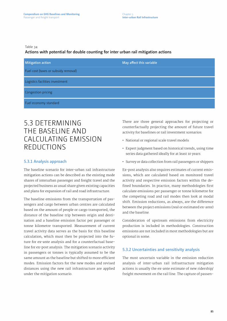
Compendium on GHG Baselines and MonitoringPassenger and freight transport
85
5.3 DETERMINING THE BASELINE AND CALCULATING EMISSION REDUCTIONS
5.3.1 Analysis approach
The baseline scenario for inter-urban rail infrastructure
mitigation actions can be described as the existing mode
shares of interurban passenger and freight travel and the
projected business as usual share given existing capacities
and plans for expansion of rail and road infrastructure.
The baseline emissions from the transportation of pas-
sengers and cargo between urban centres are calculated
based on the amount of people or cargo transported, the
distance of the baseline trip between origin and desti-
nation and a baseline emission factor per passenger or
tonne kilometre transported. Measurement of current
travel activity data serves as the basis for this baseline
calculation, which must then be projected into the fu-
ture for ex-ante analysis and for a counterfactual base-
line for ex-post analysis. The mitigation scenario activity
in passengers or tonnes is typically assumed to be the
same amount as the baseline but shifted to more efficient
modes. Emission factors for the new modes and revised
distances using the new rail infrastructure are applied
under the mitigation scenario.
There are three general approaches for projecting or
counterfactually projecting the amount of future travel
activity for baselines or rail investment scenarios:
· National or regional scale travel models
· Expert judgment based on historical trends, using time
series data gathered ideally for at least 10 years
· Survey or data collection from rail passengers or shippers
Ex-post analysis also requires estimates of current emis-
sions, which are calculated based on monitored travel
activity and respective emission factors within the de-
fined boundaries. In practice, many methodologies first
calculate emissions per passenger or tonne kilometre for
the competing road and rail modes then look at modal
shift. Emission reductions, as always, are the difference
between the project emissions (real or estimated ex-ante)
and the baseline.
Consideration of upstream emissions from electricity
production is included in methodologies. Construction
emissions are not included in most methodologies but are
optional in some.
5.3.2 Uncertainties and sensitivity analysis
The most uncertain variable in the emission reduction
analysis of inter-urban rail infrastructure mitigation
actions is usually the ex-ante estimate of new ridership/
freight movement on the rail line. The capture of passen-
Table 34
Actions with potential for double counting for inter urban rail mitigation actions
Mitigation action May affect this variable
Fuel cost (taxes or subsidy removal)
Logistics facilities investment
Congestion pricing
Fuel economy standard
Mode share of passengers or freight
Induced trips, mode share
Mode share of passengers or freight
Emission factor for road modes compared to rail
Chapter 5Inter-urban Rail Infrastructure

Compendium on GHG Baselines and MonitoringPassenger and freight transport
86
ger trips by rail mode can come from cars or from busses,
so accurate mode split data is important. For freight the
vehicle fleet (and age) of trucks is important. Predicting
mode split depends on the relative attractiveness of the
rail line to alternative modes, which is highly context de-
pendent and differs for freight and passenger situations.
In contrast, ex-post methodologies are fairly simple,
based on monitoring and assuming that the change in
mode share is due to the project.
The potential for rebound effects is also difficult to esti-
mate ex-ante, although economic models may offer some
guidance as to the elasticity of travel versus cost.
5.4 GUIDANCE ON THE SELECTION OF ANALYSIS TOOLS FOR INTER-URBAN
RAIL INFRASTRUCTURE MITIGATION ACTIONS
Higher degrees of accuracy can be obtained with more
disaggregated data, if some or all of the data is locally
derived. While combining local data with defaults can
yield benefits, using disaggregated default data alone is
seldom more accurate than aggregated default data. Table
35 shows the disaggregated data that is desirable for each
general level of accuracy.
There are a two rail specific transport analysis method-
ologies for GHG analysis under the CDM and JICA devel-
oped three more simplified methods based on CDM. The
TEEMP project has developed a rail mode shift sketch
planning module that accommodates freight or passen-
gers. In addition a methodology for monitoring a nation-
al rail programme in India was developed for the Asian
Development Bank and India Railways. Travel demand
Table 35
Level of disaggregation of key variables
Lower accuracy Medium accuracy
Degree of local data disaggregation and context variables
Higher accuracy
Travel activity data
Emission factors
• Total vehicle trips
• Forecast change
in passengers or
tonnes to rail
• Average passengers
or tonnes per road
vehicle and rail
vehicles*
• Average trip length*
• Average emission
factors *
• Vehicle trips in analysis corridor or
area by vehicle type
• Vehicle trip length by vehicle type
• Proposed change in car/bus/truck
VKT from feeder operations
• Forecast change in rail tonnage
• Emission factors by vehicle type and
speed*
• Total passenger trips or tonnes shipped in
analysis area
• PKM or TKM in analysis area by vehicle type
• Passengers or tonnes/vehicle by vehicle type
• Proposed change in VKT from feeder
operations (by vehicle type)
• Forecast change in passengers or tonnes/mode
• Trip lengths of new shifted trips by mode (incl
feeder)
• Prior mode of cargo
• Forecast change in VKT by vehicle type
(modelled)**
• Emission factors for rail vehicles
• Construction emission of new
infrastructure**
*=default OK, **= optional item) for inter urban rail mitigation actions
Chapter 5Inter-urban Rail Infrastructure

Compendium on GHG Baselines and MonitoringPassenger and freight transport
87
modelling can also be used in areas where regional or na-
tional models are available, although models for freight
are not as common as for passenger travel. Commercial
software packages have passenger and freight modelling
capabilities that include rail modes.
Figure 18 maps existing methodologies and tools for
freight modal shift projects according to their purpose (y
axis) and level of accuracy (x axis).
5.4.1 Description of tool types
The following sections describe a number of tools that
are available for estimating GHG reduction from transit
projects. They are classified according to similarities in
methodology.
Figure 18
Navigating classes of available methods and associated tools for inter-urban rail infrastructure mitigation actions
Prioritize policies
Objective
Report results
Mitigation planning
Emissions trading
Ex-a
nte
Lower accuracy Medium accuracy Higher accuracy
Ex-p
ost
Spreadsheet or software tool Guidance document
Spreadsheet tools with defaults
Cube
TransCad
Visum
EMME
TRANUS
+ local emissions models, e.g., HBEFA,
MOVES
Spreadsheet tools with local data
TEEMP Railway alternatives
CDM methodologies
Travel models
AM0090: Modal shift in transportation of cargo from road transportation to water or rail transportation
AM0101: High speed passenger rail systems
Other bottom-up methodologies/
guidanceJICA-Railway Freight Electrification
JICA-Railway Freight Mode shift
MRV Blueprint based on India Railways NAMA
Chapter 5Inter-urban Rail Infrastructure

Compendium on GHG Baselines and MonitoringPassenger and freight transport
88
5.4.2 Travel demand models
These are spatial interaction models that calculate VKT
disaggregated by mode, time of day and speed. Trip
lengths are based on location of origins and destina-
tions. Mode choice can be modelled based on interaction
of origins, destinations and transport systems. Induced
trips can be modelled using capacity restraint formula
(activity models may have more sophisticated methods).
With appropriate sub modules some models can include
freight, transit, NMT. Some models can include land use
simulations as well. Important disaggregated variables
cascade through analysis. Some defaults may be includ-
ed and models include the ability to change any variable.
Models are calibrated by entering local data from detailed
travel surveys and comparing the model output to known
results. This option is the most accurate choice for fore-
casting future travel activity parameters.
Typically, highly disaggregated activity data from travel
demand models is input to a separate emissions mod-
el calibrated to national or supra-national fleets. Some
software packages incorporate emissions factors from
various sources for an extra cost. External standard
emissions models that accept highly disaggregated in-
puts include MOVES, HBEFA, IVE, etc. Emissions models
also have to be adapted to local or at least country-spe-
cific circumstances regarding e.g., the underlying fleet
composition and emission factors to deliver meaningful
results. Travel model outputs can, however, also be ag-
gregated and emissions calculated with simpler emis-
sions factors.
5.4.3 Disaggregated bottom-up ex-post guidance
These are CDM methodology documents or other MRV
guidance documents that detail the disaggregated vari-
ables that should be collected. The documents often give
precise methodologies on how to collect these variables
and how to calculate emissions using them. Because
CDM is focused on documenting precise amounts of real
Table 36
Travel demand models for inter urban rail mitigation actionsEase of use/data collection: Highly resource and data intensive
Name Application /summary
Scope Computer based
Methodology documentation
Defaults Provided
Data collection guidance
Cost of tool
Cube
TransCad
VISUM
EMME
TRANUS
Multimodal
passenger and
truck freight
Multimodal
passenger truck
and rail freight
Multimodal
Unknown
Multimodal
passenger only
Excellent
Excellent
Excellent
Excellent
Very good
Internal
parameters*
Internal
parameters*
Internal
parameters*
Internal
parameters*
Internal
parameters*
Passengers and
commodity flow
Commodity flow
Passenger trips
and “tour based”
freight model
Travel activity
Travel activity
Yes
Yes
Yes
Yes
Yes
Paid training
offered
Paid training
offered
Paid training
offered
Paid training
offered
Fair
High
High
High
High
Free
*for example friction factors, mode choice curves, and other coefficients for internal sub-models
Chapter 5Inter-urban Rail Infrastructure

Compendium on GHG Baselines and MonitoringPassenger and freight transport
89
tonnes, CDM tools are primarily used ex-post. Ex-ante
BAU is estimated following the same general approach
but not described in detail in CDM methodologies. Some-
times induced trips may be estimated using this meth-
odology. Defaults and spreadsheets are not included, al-
though default sources may be referenced.
5.4.4 Partially aggregated bottom-up spreadsheet tools with defaults
This is a spreadsheet based tool that has the opportuni-
ty for local data to be used but also include a variety of
defaults especially for emissions factors. It offers some
Table 37
Disaggregated bottom-up ex-post guidance for inter urban rail mitigation actionsEase of use/data collection: Moderately resource and data intensive
Name Application /summary
Scope Computer based
Methodology documentation
Defaults Provided
Data collection guidance
Cost of tool
MRV-Blueprint: India Railways NAMA
AM00090 Proposed Version 03.1
AM0101 High speed passenger rail systems
Passenger and
freight mode
shift from road
or air modes
Ex-post,
upstream
including
construction,
electric grid
factor
Ex-post,
upstream electric
grid factor,
includes shift
from air travel
Very good
Good
Very good
No
Defaults emis-
sion factors for
diesel for trucks,
barges and ship
fuel oils
Default emission
factors for air
travel
National rail
infrastructure
programme
NAMA
Shift cargo
among trucks
barges, ships
and trains
Passenger rail
system >200kph
No
No
No
Good, brief
recommen-
dations for
data sources at
national level
Brief
“measurement
procedures”
for all variables
Very good
Free
Free
Free
Table 38
Partially aggregated bottom-up spreadsheet tools with defaults for inter urban rail mitigation actionsEase of use/data collection: Moderate
Name Application /summary
Scope Computer based
Methodology documentation
Defaults Provided
Data collection guidance
Cost of tool
TEEMP Railway alternatives
Manual entry of
expected mode
shift by percent
General guide for
all spreadsheets
Emission factors
for passenger
and tonne
kilometre for
highway and rail
Defaults for trip
lengths
Rough ex-ante
assessment
based on shift
of passengers
and/or freight
between road
and rail
Yes Some
guidance with
defaults
Free
Chapter 5Inter-urban Rail Infrastructure

Compendium on GHG Baselines and MonitoringPassenger and freight transport
90
limited methods for estimating future VKT, mode share
or ridership.
5.4.4 Simple Aggregated bottom-up guidance tools
These are guidance documents that offer a framework of
equations for calculating GHG reduction from mode shift.
5.5 MONITORING
Performance of the mitigation action should be monitored
by tracking key variables over time. The monitoring fre-
quency will vary, depending on the monitoring regimen
and the budget available for data collection. Official pas-
senger and freight data should be obtained from railway
operators, which may or may not be government owned
depending on the national circumstances. Key mode share
and trip length data can require transport surveys that
may not be possible on an annual or biannual basis. Al-
though new methods such as mobile phone tracking can
substitute for surveys in some instances, many organiza-
tions cannot be assumed to have reliable data for all varia-
bles annually. However different variables can be updated
at different intervals.
Implementation and performance data can show progress
before the full effects of the action may be apparent. The
table below presents a minimum list of key variables and
recommended maximum intervals for measurement if no
other requirements are present, (e.g., CDM).
5.6 EXAMPLE - INDIA RAILWAY NAMA
A methodology was developed for MRV of a national lev-
el railway NAMA. The NAMA includes six dedicated freight
Table 39
Simple bottom-up tools with mostly default data for inter urban rail mitigation actionsEase of use/data collection: Moderate to low
Name Application /summary
Scope Computer based
Methodology documentation
Defaults Provided
Data collection guidance
Cost of tool
JICA Rail-way electri-fication
JICA Railway (Freight) mode shift
JICA Railway passenger mode shift
Includes mode
shift effects
Includes
upstream grid
factor
Includes
upstream grid
factor
Includes mode
shift effects
Includes up-
stream grid factor
Limited
Limited
Limited
Refers to
appendix
Refers to
appendix
Refers to
appendix
GHG reduction
from
electrification
of rail
Mode shift of
freight from
truck to rail
Aimed more at
within urban ar-
eas but works for
inter urban rail
No
No
No
Fair
Fair
Fair
Free
Free
Free
Chapter 5Inter-urban Rail Infrastructure

Compendium on GHG Baselines and MonitoringPassenger and freight transport
91
corridors, double, triple or four tracking of various saturat-
ed corridors and technology upgrades and new rolling stock.
Total investment of nearly $800 billion USD is contemplated.
The MRV methodology looks at the entire rail sector cover-
ing all inter urban rail operations in India. Urban services
are not included. It looks at direct and indirect effects in-
cluding construction and upstream fuel production. Two
baselines are examined, a frozen baseline and a dynamic
BAU with some rail growth. The ex-ante estimate for the
entire NAMA using the “frozen” baseline is a reduction of
152 MtCO2 per annum between 2012 and 2030.
Further details are available at:
http://transport-namas.org/wp-content/uploads/2014/10/
TRANSfer_MRV-Blueprint_Railway-NAMA_India_draft.pdf
Table 40
Minimum indicator set for Inter urban rail mitigation action
Category Indicator Normal monitoring frequency
Implementation indicator
Performance indicators
Impact indicators
Completion of new rail line or facility
Mode shift in percent
Annual passengers or tonnes of cargo by mode
Calculated passenger or cargo tonne kilometres by mode
Latest emission rates by mode
Calculated emissions in study area
Onetime or by construction phase
Annual
Annual
5 years
5 years
5 years
Chapter 5Inter-urban Rail Infrastructure

Compendium on GHG Baselines and MonitoringPassenger and freight transport
92
Chapter 6
SHIFT MODE OF FREIGHT TRANSPORT FROM ROAD TO RAIL OR WATER

Compendium on GHG Baselines and MonitoringPassenger and freight transport
93
6.1 DESCRIPTION AND CHARACTERISTICS OF FREIGHT MODAL SHIFT MITIGATION ACTIONS
This mitigation action includes activities that result in
modal shift in transportation of a specific cargo (exclud-
ing passengers) from road transportation using trucks to
water transportation using barges or ships or rail trans-
portation.
This mitigation action covers investments that increase
the capacity and/or decrease the cost of rail or water
transport modes. This typically includes infrastructure
such as rail lines, station or yards and rolling stock as well
as intermodal rail hubs and port facilities, river channel
projects, ship or barge fleets, etc. The investments may
include new vehicles that are more efficient than the old
fleet, which increases the emission reduction effect of the
modal shift.
The outcomes of successful implementation of this mit-
igation action are expected to decrease mode share of
truck cargo and increase rail or water borne cargo share,
in some cases for a specific type of cargo as freight shift
is highly dependent upon the type of good. This leads to
decreased tonne/kilometres moved by truck, decreased
truck VKT and a shift of those tonne kilometres to more
efficient rail or water modes, resulting in decreased fuel
use and GHG emissions
Shifting freight from truck modes to rail or water can
generate sustainable development co-benefits such as
decreased congestion and noise due to fewer trucks on the
road. It can also lead to increased road safety by reducing
traffic. Reduced toxic air pollution can also be a benefit,
especially if freight is moved to electric rail.
6.2 STRUCTURE OF MITIGATION EFFECTS
6.2.1 Cause-impact chain
Freight mode-shift actions result in measurable effects
reflected in ASIF indicators, but the causal chain model is
slightly different from passenger transport. Mitigation ac-
tions in the form of investments in new infrastructure in
essence reduce the cost per unit of transporting freight us-
ing the target modes. However many factors go into the cost
calculation. The actual choice of mode is based on a com-
bination of four categories of cost factors described below:
1. Goods Characteristics – These include physical charac-
teristics of goods such as the type of commodity, the
size of the shipments, weight, density and the value of
the goods;
2. Modal Characteristics – Speed of the mode, mode relia-
bility, network accessibility and the capacity;
3. Total Logistics Cost – Inventory costs, loss and damage
costs, and service reliability costs; and
4. Overall Logistics Characteristics – Length of haul and
the shipment frequency, intermodal transfers and fee-
der trips, empty return trips or repositioning of empty
containers
Trip length depends on the origin and destination of the
specific type of freight that is transported. Similarly the load
factor will vary with the type of freight and the mode chosen.
If the elasticity of demand is sufficient the decreased “cost”
can result in increased total freight and more economic ac-
tivity as a rebound effect, eroding some of the GHG benefits.
The expected changes in those variables will cause the de-
sired outcomes. See Figure 19.
Chapter 6Shift mode of freight transport from road to rail or water
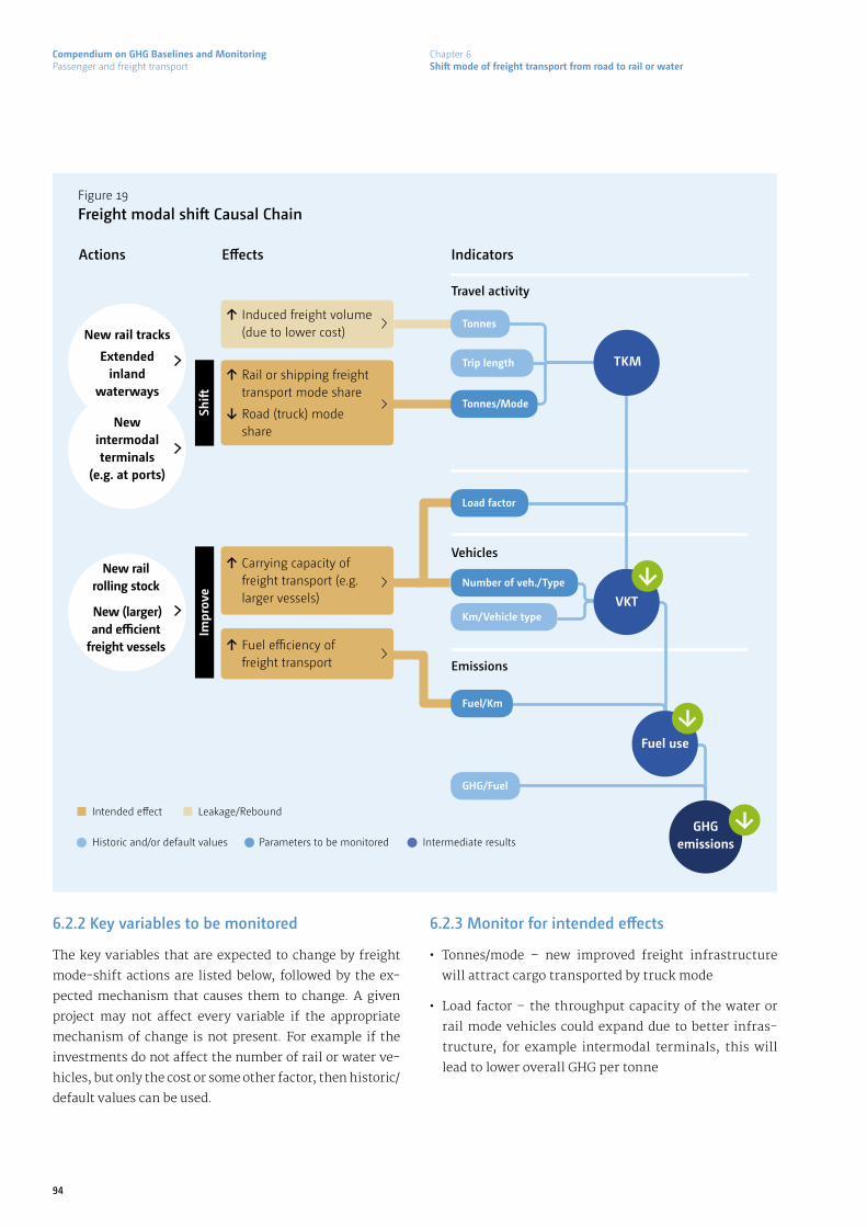
Compendium on GHG Baselines and MonitoringPassenger and freight transport
94
Figure 19
Freight modal shift Causal Chain
Actions Effects Indicators
New rail rolling stock
New (larger) and efficient
freight vessels
↑ Induced freight volume (due to lower cost)
↑ Rail or shipping freight transport mode share
↓ Road (truck) mode share
↑ Carrying capacity of freight transport (e.g. larger vessels)
↑ Fuel efficiency of freight transport
Travel activity
Vehicles
Emissions
Shift
Impr
ove
TKM
Load factor
Tonnes
Trip length
Tonnes/Mode
Km/Vehicle type
GHG emissions
Intended effect Leakage/Rebound
Historic and/or default values Intermediate resultsParameters to be monitored
Fuel/Km
GHG/Fuel
New intermodal terminals
(e.g. at ports)
New rail tracks
Extended inland
waterways
Number of veh./Type
VKT
Fuel use
6.2.2 Key variables to be monitored
The key variables that are expected to change by freight
mode-shift actions are listed below, followed by the ex-
pected mechanism that causes them to change. A given
project may not affect every variable if the appropriate
mechanism of change is not present. For example if the
investments do not affect the number of rail or water ve-
hicles, but only the cost or some other factor, then historic/
default values can be used.
6.2.3 Monitor for intended effects
· Tonnes/mode – new improved freight infrastructure
will attract cargo transported by truck mode
· Load factor – the throughput capacity of the water or
rail mode vehicles could expand due to better infras-
tructure, for example intermodal terminals, this will
lead to lower overall GHG per tonne
Chapter 6Shift mode of freight transport from road to rail or water
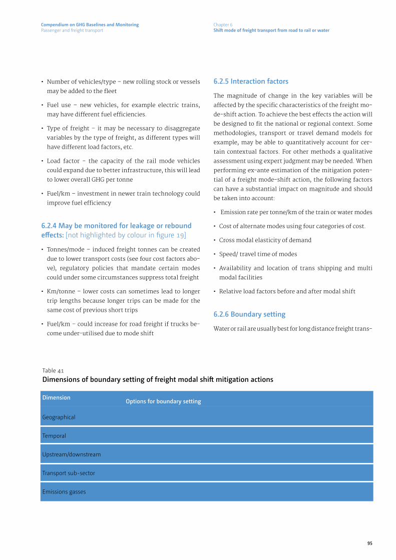
Compendium on GHG Baselines and MonitoringPassenger and freight transport
95
· Number of vehicles/type – new rolling stock or vessels
may be added to the fleet
· Fuel use – new vehicles, for example electric trains,
may have different fuel efficiencies.
· Type of freight – it may be necessary to disaggregate
variables by the type of freight, as different types will
have different load factors, etc.
· Load factor - the capacity of the rail mode vehicles
could expand due to better infrastructure, this will lead
to lower overall GHG per tonne
· Fuel/km – investment in newer train technology could
improve fuel efficiency
6.2.4 May be monitored for leakage or rebound effects: [not highlighted by colour in figure 19]
· Tonnes/mode – induced freight tonnes can be created
due to lower transport costs (see four cost factors abo-
ve), regulatory policies that mandate certain modes
could under some circumstances suppress total freight
· Km/tonne – lower costs can sometimes lead to longer
trip lengths because longer trips can be made for the
same cost of previous short trips
· Fuel/km – could increase for road freight if trucks be-
come under-utilised due to mode shift
6.2.5 Interaction factors
The magnitude of change in the key variables will be
affected by the specific characteristics of the freight mo-
de-shift action. To achieve the best effects the action will
be designed to fit the national or regional context. Some
methodologies, transport or travel demand models for
example, may be able to quantitatively account for cer-
tain contextual factors. For other methods a qualitative
assessment using expert judgment may be needed. When
performing ex-ante estimation of the mitigation poten-
tial of a freight mode-shift action, the following factors
can have a substantial impact on magnitude and should
be taken into account:
· Emission rate per tonne/km of the train or water modes
· Cost of alternate modes using four categories of cost.
· Cross modal elasticity of demand
· Speed/ travel time of modes
· Availability and location of trans shipping and multi
modal facilities
· Relative load factors before and after modal shift
6.2.6 Boundary setting
Water or rail are usually best for long distance freight trans-
Table 41
Dimensions of boundary setting of freight modal shift mitigation actions
DimensionOptions for boundary setting
Geographical
Temporal
Upstream/downstream
Transport sub-sector
Emissions gasses
National, regional, specific freight corridor
10-20 years
Energy sector (conventional fuels, electricity, biofuels), may also consider infrastructure construction
Freight transport
CO2e (may include CH4, N2O )
Chapter 6Shift mode of freight transport from road to rail or water

Compendium on GHG Baselines and MonitoringPassenger and freight transport
96
issues to consider when selecting a methodology include:
· Attributing shift to particular policy or investment –
how much does that policy affect the mode choice com-
pared to other factors.
· Determining if the cargo would have gone by truck wi-
thout project – some cargo will naturally go by water or
rail due to bulk, non-time-sensitivity, etc.
· Using correct emissions factors for rail or ship – are de-
fault factors appropriate or are local emission factors
per kilometre or per tonne different than typical values
due to unique vehicles or geography, feeder require-
ments, etc.? If electric rail is used CO2 emission factors
of grid electricity specific to the national or regional
grid have to be used.
· Accounting for truck feeder transport to and from rail
or ship. If there is a substantial cost savings for water or
rail, cargo may be attracted from more distant areas via
feeder trucks.
· Specific characteristics of the non-road modes including
empty return factors, size of vessels (larger vessels may
have adverse environmental impacts such as river dre-
dging, pollution from dirty bunker fuels, etc., leading to
political opposition).
6.2.8 Double counting concerns
Other policies and actions taken to mitigate GHG may
have synergistic or interaction effects on freight mode
Table 42
Actions with potential for double counting of freight modal shift mitigation actions
Mitigation action May affect this variable
Fuel cost (taxes or subsidy removal)
Logistics facilities investment
Fuel economy standards or measures for trucks
Improved logistics practices (e.g., alliances of small truckers)
Mode share
Induced trips, mode share
Mode share, truck transport costs
Mode share, truck transport costs
port, thus the project will be best analysed at the national
or regional level. Often a specific corridor such as a river is
singled out for investment, which can be used as the boun-
dary while considering the feeder routes leading into it.
Upstream emissions from electricity generation should be
included if the rail is powered electrically. However if the
mitigation action of the project aims solely at the switch to
electric energy, that is if rail freight is part of the baseline
and the only difference is energy source, then the analysis
should consider methodologies under Fuel switching (ac-
tion type 4).
Large projects such as a port or new rail lines and yards
may have substantial construction emissions, which
should be considered as part of the lifecycle emissions and
factored into calculations. In this case it may be necessary
to compare to baseline construction emissions if the BAU
scenario includes new highways or similar investments.
6.2.7 Key methodological issues
The GHG impact depends on the specifics of the project
that make water or rail a more viable choice for freight
transport compared to truck. These need to be considered
carefully in any ex-ante analysis. Variables pertaining to
the value of the freight, the time sensitivity and the loca-
tion of origins and destinations become important when
estimating the potential for mode shifting. Consideration
of the end distribution characteristics of the cargo, for
example whether it is delivered to a single factory or to
multiple small stores, also affects the mode choice. Other
Chapter 6Shift mode of freight transport from road to rail or water

Compendium on GHG Baselines and MonitoringPassenger and freight transport
97
shift actions. This can lead to difficulty in attributing the
reduction to a particular action or to counting the same
tonnes more than once for different actions. Care should
be taken in this regard if any of the following policies
or actions is being implemented concurrently with the
freight mode-shift action.
6.3 DETERMINING THE BASELINE AND CALCULATING EMISSION REDUCTIONS
6.3.1 Analysis approach
The baseline scenario for freight mode shift actions is
that the freight is transported by trucks over roadways.
The baseline emissions from the transportation of the
cargo are calculated based on the amount of cargo trans-
ported, the distance of the baseline trip between origin
and destination for transportation of cargo by trucks and
a baseline emission factor per tonne-km of cargo trans-
ported. Measurement of current freight movement data
serves as the basis for this baseline calculation, which
must then be projected into the future for ex-ante anal-
ysis and counterfactually projected for ex-post analysis.
The mitigation scenario freight activity in tonne-kms is
typically assumed to be the same amount as the baseline
but shifted to more efficient modes. Emission factors for
the new modes and revised distances are applied under
the mitigation scenario.
There are four general approaches for projecting or coun-
terfactually projecting the amount of future freight ac-
tivity for baselines or mode shift scenarios:
· National or regional freight models – based on commo-
dity flow and/or spatial inputs
· Growth factor methods based on direct economic
projections
· Expert judgment based on historical trends, using time
series data gathered ideally for at least 10 years
· Survey or data collection from shippers including sta-
ted preference surveys.
Ex-post analysis also requires estimates of current emis-
sions, which are calculated based on the measured freight
movements and respective emission factors within the
defined boundaries. In practice, many methodologies de-
termine emissions per tonne kilometre of freight (includ-
ing return factors) for various modes then look at modal
shift. Emission reductions, as always, are the difference
between the project emissions (real or estimated ex-ante)
and the baseline.
Consideration of upstream emissions from electricity
production is included in methodologies. Construction
emissions are not included in some methodologies but
are optional in others.
6.3.2 Uncertainties and sensitivity analysis
The most uncertain variable in the emission reduc-
tion analysis of freight mode shift projects is usually
the ex-ante estimate of mode split and demand for new
freight activity. Mode split depends on the relative at-
tractiveness to shippers of the various modes and can
vary depending on the type of cargo. Demand can be
projected by commodity production models in developed
countries, but such data is often very uncertain in dy-
namically developing countries. Different methodologies
address baseline setting in various ways to accommodate
this uncertainty.
In contrast, ex-post methodologies are fairly simple, as-
suming that the change in mode share is due to the project.
The potential for rebound effects is also difficult to esti-
mate ex-ante, although economic models may offer some
guidance as to the elasticity of freight transport versus
generalised cost.
Chapter 6Shift mode of freight transport from road to rail or water

Compendium on GHG Baselines and MonitoringPassenger and freight transport
98
6.4 GUIDANCE ON THE SELECTION OF ANALYSIS TOOLS FOR FREIGHT MODAL SHIFT PROJECTS
Higher degrees of accuracy can be obtained with more
disaggregated data, if some or all of the data is locally de-
rived. While combining local data with defaults can yield
benefits, using disaggregated default data alone is seldom
more accurate than aggregated default data. The table
above shows the disaggregated data that is desirable for
each general level of accuracy.
There are a few freight transport analysis methodologies
for GHG analysis under the CDM. The TEEMP project has
also developed a rail mode shift sketch planning module
that accommodates freight. Transport demand modelling
practice for freight is not as widespread as for passen-
ger travel, although commercial software packages have
freight capabilities that include rail.
Figure 20 maps existing methodologies and tools for
freight modal shift projects according to their purpose (y
axis) and level of accuracy (x axis).
6.4.1 Description of tool types
The following sections describe a number of tools that
are available for estimating GHG reduction from freight
mode shift mitigation actions. They are classified accord-
ing to similarities in methodology.
6.4.2 Freight demand models
Freight demand is mostly found as a component of a larg-
er travel demand forecasting model. The freight com-
Table 43
Level of disaggregation of key variables of freight modal shift mitigation actions
Lower accuracy Medium accuracy
Degree of local data disaggregation and context variables
Higher accuracy
Transport activity
data
Emission factors
• Total freight vehicle trips
• Forecast change in truck
tonne-kms to rail or
ship
• Average tonnes per truck
and rail/ship vehicles*
• Average trip length*
• Average emission factors
per tonne-km *
• Freight vehicle trips in analysis
area by vehicle type
• Freight vehicle trip length by
vehicle type
• Proposed change in truck VKT
from feeder operations
• Forecast change in rail or ship
tonnage
• Emission factors by vehicle type
and speed*
• Total tonnes shipped in analysis area
• TKM in analysis area by vehicle type
• Tonnes/vehicle by vehicle type
• Proposed change in freight VKT from operations
(by vehicle type)
• Forecast change in tonnes/mode
• Trip lengths of new freight trips by mode (incl feeder)
• Prior mode of cargo
• Forecast change in truck VKT by vehicle type
(modeled)**
• Emission factors for rail or ship vehicles
• Construction emission of new
infrastructure**
*=default OK, **= optional item)
Chapter 6Shift mode of freight transport from road to rail or water

Compendium on GHG Baselines and MonitoringPassenger and freight transport
99
ponents typically focus on truck flows to forecast the
demand for intercity corridors or for regional systems
planning. Some national or state level government agen-
cies will prepare a commodity-based freight model. This
methodology uses flows of commodities between various
industries to be reflected through a series of freight deci-
sion-making models resulting in flows of trucks, trains,
etc. Commercial travel modelling software such as Cube
or TransCad can be used to develop commodity genera-
tion and distribution models based on employment fac-
tors or other industry data. Such models may also have
multi-modal capabilities to allocate freight to the various
cargo transport modes.
Chapter 6Shift mode of freight transport from road to rail or water
Figure 20
Navigating classes of available methods and associated tools of freight modal shift mitigation actions
Prioritize policies
Objective
Report results
Mitigation planning
Emissions trading
Ex-a
nte
Lower accuracy Medium accuracy Higher accuracy
Ex-p
ost
Spreadsheet or software tool Guidance document
Spreadsheet tools with defaults
Cube
TransCad
Visum
EMME
+ local emissions models, e.g., HBEFA,
MOVESSpreadsheet tools with local data
CCAP Emissions Guidebook
CDM methodologies
Travel models
AM00090: Proposed Version 03.1
CDM Tool 17*
AM0110*
Other bottom-up methodologies/
guidanceJICA Railway electrification
JICA Railway (Freight) mode shift
TEEMP Railway alternatives
(*) CDM Tool 17: Baseline emissions for modal shift measures in inter urban cargo transport; AM0090: Modal shift of cargo from road to water or rail transportation; AM0110: Large-scale Methodology: Modal shift in transportation of liquid fuels Version 01.0.0

Compendium on GHG Baselines and MonitoringPassenger and freight transport
100
As with passenger models, disaggregated activity data from
freight demand models is input to a separate emissions
model calibrated to national or supra-national fleets. In
this case the emissions model should be adapted to specific
circumstances regarding the underlying fleet composition.
Travel model outputs can, however, also be aggregated and
emissions calculated with simpler emissions factors..
6.4.3 Disaggregated bottom-up ex-post guidance
These are CDM methodology documents or general guid-
ance documents that provide formulas for GHG emissions
calculations and detail the disaggregated variables that
should be collected. The documents often also supply
methodologies on how to collect these variables, empha-
sizing the most conservative assumptions. Because CDM
is focused on documenting precise amounts of real tonnes,
CDM tools are primarily used ex-post. Users are referred
to the Combined tool to identify the baseline scenario and
demonstrate additionality for general ex-ante guidance.
Some defaults are included. No spreadsheet is provided.
6.4.4 Partially aggregated bottom-up spreadsheet tools with defaults
This is a spreadsheet based tool developed for ex-ante
estimation that has the opportunity for local data to be
used but also includes a variety of defaults especially for
emissions factors.
6.4.5 Aggregated bottom-up guidance tools
These are guidance documents that offer a framework of
equations for calculating GHG reduction from mode shift.
One is specific to electrification of rail lines including
new or existing electric rail, the other is more general
and offers guidance for monitoring any action designed
to increase rail mode of freight.
Table 44
Travel demand models for freight modal shift mitigation actionsEase of use/data collection: Highly resource and data intensive
Name Application /summary
Scope Computer based
Methodology documentation
Defaults Provided
Data collection guidance
Cost of tool
Cube
TransCad
VISUM
EMME
Truck
Truck and rail
Multimodal
Unknown
Excellent
Excellent
Excellent
Excellent
Internal
parameters*
Internal
parameters*
Internal
parameters*
Internal
parameters*
Commodity flow
Commodity flow
“Tour based”
freight model
Travel activity
Yes
Yes
Yes
Yes
Paid training
offered
Paid training
offered
Paid training
offered
Paid training
offered
High
High
High
High
*for example friction factors, mode choice curves, and other coefficients for internal sub-models
Chapter 6Shift mode of freight transport from road to rail or water

Compendium on GHG Baselines and MonitoringPassenger and freight transport
101
Table 45
Travel demand models for freight modal shift mitigation actionsEase of use/data collection: Highly resource and data intensive
Name Application /summary
Scope Computer based
Methodology documenta-tion
Defaults Provided
Data collection guidance
Cost of tool
AM00090 Proposed Version 03.1
CDM Tool 17: Baseline emis-sions for modal shift measures in inter urban cargo transport
MRV-Blueprint: India Railways NAMA
AM0110Large-scale Methodology: Modal shift in transportation of liquid fuelsVersion 01.0.0
Ex-post, upstream
including construction,
electric grid factor
Ex-post, no upstream
emissions except elec-
tric grid factor
Passenger and freight
mode shift from road
or air modes
Ex-post, includes
upstream electric emis-
sions, trucks to trans-
port fuel for pipeline
and land use changes
from pipeline
Good
Good
Very Good
Good
Defaults emission
factors for diesel
for trucks, barges
and ship fuel oils
Default emission
factors for rail,
water and road
disaggregated by
some cargo types
No
Includes a single
default value for
truck fuels
Shift cargo among
trucks barges, ships
and trains
modal shift from
road to water-borne
(using barges or
domestic ships) or
rail transportation
National rail
infrastructure
programme NAMA
Shift in mode of
transportation of liq-
uid fuels from road
transportation using
trucks to pipeline
transportation.
No
No
No
No
Brief “Measure-
ment proce-
dures” for all
variables
Brief “Measure-
ment proce-
dures” for only
some variables
Good, brief rec-
ommendations
for data sources
at national level
Brief “Measure-
ment proce-
dures” for only
some variables
Free
High
High
High
Chapter 6Shift mode of freight transport from road to rail or water
Table 46
Partially aggregated bottom-up spreadsheet tools with defaults for freight modal shift mitigation actionsEase of use/data collection – moderate
Name Application /summary
Scope Computer based
Methodology documentation
Defaults Pro-vided
Data collection guidance
Cost of tool
TEEMP Railway alternatives
Manual entry of
expected mode
shift by percent
General guide for
all spreadsheets
Emission factors
for passenger and
tonne kilometre for
highway and rail
Defaults for trip
lengths
Shift of
passengers
and/or freight
between road
and rail
Yes Some guid-
ance with
defaults
Free

Compendium on GHG Baselines and MonitoringPassenger and freight transport
102
Chapter 6Shift mode of freight transport from road to rail or water
Table 47
Simple bottom-up tools with mostly default data for freight modal shift mitigation actionsEase of use/data collection: Moderate to low
Name Application /summary
Scope Computer based
Methodology documentation
Defaults Provided
Data collection guidance
Cost of tool
JICA Rail-way electri-fication
JICA Railway (Freight) mode shift
CCAP Emissions Guidebook
Includes mode
shift effects
Includes up-
stream grid factor
Includes
upstream grid
factor
Ex-ante tool;
sketch planning
estimates based
on reduction in
number of trucks
(and/or change
in loading)
Limited
Limited
Good
Refers to
appendix
Refers to
appendix
US energy and
emission factors
for trucks
GHG reduction
from electrifica-
tion of rail
Mode shift of
freight from
truck to rail
Mode shift from
truck to rail or
barge
No
No
No
Fair
Fair
Fair
Free
Free
Free
6.5 MONITORING
Performance of the mitigation action can be monitored by
tracking key variables over time. The monitoring frequen-
cy will vary, depending on the monitoring regime and the
budget available for data collection.
Implementation and performance metrics should be in-
cluded in the monitoring plan to show progress before the
full effects of the action may be apparent. Freight move-
ment is generally done by private companies so proprie-
tary data may need to be requested for monitoring pur-
poses. If this is not available default data will have to be
found. Official government statistics can be used if they
are deemed transparent and reliable and offer the degree
of disaggregation required. Incentives for carriers to re-
port data should be considered, as proprietary data for to-
tal tonnes moved by mode, and fuel use by mode will pro-
vide the most accurate estimates.
The table below presents a minimum list of key variables
and recommended maximum intervals for measurement
if no other requirements are present, (e.g., CDM).

Compendium on GHG Baselines and MonitoringPassenger and freight transport
103
6.6 EXAMPLE – SWITCHING FREIGHT TO SHORT SEA SHIPPING (BRAZIL)
An example of a freight mode shift project was the develop-
ment of waterway infrastructure to shift freight transport
from road to waterways. This project had been developed
and implemented in Brazil by ArcelorMittal Tubarão, a com-
pany specializing in the production of slabs and hot rolled
steel coils. CDM methodology AM0090 was chosen as the
method to estimate mitigation outcomes from the Arce-
lorMittal Tubarão project. According to this methodology,
annual tonne-kilometres of cargo transported by the newly
developed infrastructure were monitored and used to esti-
mate baseline and project emissions.
Baseline emissions were estimated using the following var-
iables: transportation distance (from origin to destination
point) by road using trucks, baseline emissions factor and
cargo volume (assuming the same amount of cargo trans-
ported by the newly developed infrastructure). Baseline
emissions factor was a default emissions factor in gCO2/
tonne-kilometre available in the AM0090 methodology
Data on the consumption of fuel by ocean barges was mon-
itored along with the amount of cargo transported by the
barges. The two amounts are multiplied to estimate base-
line emissions, as described above. The difference between
project emissions and baseline emissions equals the emis-
sions reductions that the implementation of the project
brings about.
The project shifts the transportation of around 1.100.000
tonnes of coils per year from road transportation by trucks
to ocean shipping by barges, leading to estimated emissions
reductions of around 120.000 tonnes of CO2/year.
Further details are available at:
http://cdm.unfccc.int/methodologies/PAmethodologies/pnm/
byref/NM0320
Table 48
Minimum indicator set for freight modal shift mitigation actions
Category Indicator Normal monitoring frequency
Implementation indicator
Performance indicators
Impact indicators
Construction of new rail or water infrastructure
Mode shift in percent
Annual tonnes of cargo by mode
Calculated passenger or cargo tonne kilometres by mode
Latest emission rates by mode
Calculated emissions in study area
Onetime or by construction phase
Annual
Annual
5 years
5 years
5 years
Chapter 6Shift mode of freight transport from road to rail or water

Compendium on GHG Baselines and MonitoringPassenger and freight transport
104
Chapter 7
NATIONAL FUEL ECONOMY STANDARD

Compendium on GHG Baselines and MonitoringPassenger and freight transport
105
7.1 DESCRIPTION AND CHARACTERISTICS OF GHG/FE STANDARDS FOR LIGHT-DUTY VEHICLES
One of the main instruments available to policymakers to
achieve significant improvements in fuel economy from
light-duty vehicles (LDVs) is through implementation of
fuel economy (FE) or greenhouse gas (GHG) emissions
standards regulations. These standards require new LDVs
to achieve lower fuel consumption and emissions over
time through continued development and application of
efficiency technologies. Adoption of such standards re-
sults in a market shift towards vehicles that are increas-
ingly fuel-efficient, consuming less fuel per kilometre
driven and thus emitting less GHG.
GHG and FE standards are set based on a vehicle attrib-
ute—typically either the size or the weight. Each auto-
motive manufacturer should meet a target value based on
the LDV fleet that it sells; compliance with the target by
each manufacturer ensures that the entire national fleet
of new vehicles achieves the desired reductions in GHG
emissions and fuel use. Because targets are designed with
increased stringency over time, the fleet becomes more
efficient every year. In addition, because the standards
mandate no specific technology, fuel, or vehicle type/size,
Figure 21
Passenger car sales CO2 emission targets and sales weighted averaged actual fleet historical performance (ICCT, 2016)
Historical performance Enacted targets Proposed targets or targets under study
Year
180
180
180
Gra
ms
CO2p
er k
ilom
eter
, nor
mal
ized
to
NED
C
Lite
rs p
er 1
00 k
ilom
eter
s (g
asol
ine
equ
ival
ent)
120
140
160
100
80
60
40
20
0 0
2025
2000
2020
2010
2005
2015
Japan 2020: 122*
S. Korea 2020: 97
Brazil 2017: 138
Mexico 2016: 145
KSA 2020: 142
China 2020: 117
US 2025: 97Canada 2025: 97
EU 2021: 95
India 2022: 113
9
8
7
5
4
3
2
1
6
(*) Note that Japan has already exceed its 2020 statutory target, as of 2013
Chapter 7National Fuel Economy Standard

Compendium on GHG Baselines and MonitoringPassenger and freight transport
106
manufacturers can choose the technology pathway that is
most suitable to their business plan while respecting local
consumer preferences.
New LDV GHG emission and FE standards regulations are
policies typically set at the national level. The regulated
entities are vehicle manufacturers and importers of all
new vehicles intended for sale within the country. These
regulations typically span 3 to 8 years, and additional reg-
ulatory phases are commonly applied to continue the pol-
icies. Figure 21 shows the evolution of sales weighted car-
bon dioxide (CO2) emissions from the passenger car fleets
of ten countries with GHG or FE standards in place today.
Successful implementation of new vehicle GHG/FE stand-
ards means that more efficient vehicles are incorporat-
ed into the fleet, thereby reducing the fleet average fuel
consumption. Globally, the application of stringent GHG/
FE standards in key regions is expected to attenuate and
even offset growth in vehicle activity and vehicle numbers
to reduce overall GHG emissions from the transportation
sector. The methodology presented in this section for
the monitoring, reporting and verification of such stand-
ards considers both the ex-ante definition of new vehicle
standards and the ex-post assessment of how standards
are impacting actual GHG emissions.
7.2 STRUCTURE OF MITIGATION EFFECTS
7.2.1 Cause-impact chain
Adoption of new vehicle GHG/FE standards brings measur-
able reductions on GHG emissions and fuel consumption for
the average light-duty vehicle via increased adoption of fuel
efficient technologies. This improvement, coupled with new
vehicle sales –which has been showing significant growth
in most emerging economies, and activity, have the poten-
tial to significantly reduce fleetwide GHG emission com-
pared to business-as-usual (BAU) conditions; those reduc-
tions can be assessed applying bottom-up models based on
CO2 emission factors, number of vehicles, and vehicle activ-
ity. This measurable fuel consumption and GHG reduction
found in regulated average new vehicles would reduce the
overall vehicle fleet GHG impact as described in Figure 22.
Adopting new vehicle GHG/FE standards regulations would
provide the following direct and indirect benefits with re-
spect to the baseline scenario:
Box 4
Vehicle energy measurement units
Many metrics can be used to describe the amount of fuel, energy and GHG emissions generated by unit of distance traveled by
a vehicle. Selection of the metric is driven by the intention of the policy to either reduce fuel use or GHG emissions (e.g., as part
of NAMAs).
Fuel economy measures distance traveled per unit of fuel consumed. The most common metrics are kilometers per liter (km/L)
and miles per gallon (mpg) in the U.S.
Fuel consumption is the reciprocal of fuel economy, and measures fuel consumed per distance traveled. It is usually expressed
in liters per 100 kilometers (L/100 km), and it is used in Europe, for example.
GHG/CO2 emissions measures GHG or CO2 emissions per distance traveled, expressed as grams of pollutant per kilometer or
mile. The metric can be expressed in grams of CO2 or CO2-equivalent per unit distance (gCO2/km or gCO2e/km). A CO2-equivalent
(CO2e) metric incorporates emissions of non-CO2 pollutants, using the global warming potential (GWP) to translate their impact
to CO2 equivalency. Primary GHGs besides CO2 are methane (CH4), nitrous oxide (N2O), and fluorinated gases (F-gases).
Energy consumption (EC) measures the energy consumed per distance traveled, for example in megajoules per kilometer
(MJ/km). Despite being a less common metric, it is relevant as a fuel-neutral metric across different fuel types and vehicle
technologies. Vehicle energy consumption is the metric used in Brazil’s vehicle efficiency standards policy.
Chapter 7National Fuel Economy Standard

Compendium on GHG Baselines and MonitoringPassenger and freight transport
107
· Reduce the fleet average emission of CO2 and fuel con-
sumed per kilometer driven for the fleet covered.
· Reduce the total annual contribution of GHG emissions
from the transport sector.
· Reduce fuel consumption from the transportation sector
and potentially fuel imports.
· Reduce emissions of GHG and pollutants generated by oil
extraction, fuel production, and distribution.
· Accelerate adoption of advanced efficiency technologies
and potentially incentivize transition to electric mobil-
ity and zero emissions. As the standards become more
stringent over time, the most advanced fuel-efficient
technologies are required. Estimates by EPA in the US
show that the most stringent GHG/FE standards in 2025
would require increased adoption of hybrid and bat-
tery electric vehicles to meet future standards (US EPA,
2016). Other complementary policy instruments can be
deployed to increase the rate of adoption via direct tax-
ation incentives or indirect incentives such as easier ac-
cess to high occupancy lanes or parking spots.
Figure 22
New vehicle fuel economy and greenhouse gas emission standards Causal Chain
Actions Effects Indicators
New light-duty vehicle
GHG/FE standards
↑ Fuel efficiency from new light-duty vehicles
Trips
Vehicles
Emissions
Impr
ove
PKM
Number of veh./Type
Persons
Trips/Person
Km/Trip
Trips/Mode
Km/Vehicle typeVKT
GHG emissions
Fuel use
Intended effect Leakage/Rebound
Fuel/Km
GHG/Fuel
Historic and/or default values Intermediate resultsParameters to be monitored
↑ Induced activity from lower fuel operating costs
Load factor/Occupancy
Chapter 7National Fuel Economy Standard

Compendium on GHG Baselines and MonitoringPassenger and freight transport
108
7.2.2 Key variables to be monitored
GHG/FE standards refer to a GHG or fuel efficiency target
level to be achieved by vehicle manufacturers in a given
year. Manufacturers and importers are the regulated en-
tities. Applying the regulations to a reduced set of stake-
holders rather than individual consumers both ensures
compliance and simplifies enforcement of the standards.
Thus, the key variable to be monitored when designing and
implementing a new vehicle GHG/FE standard is the per-
formance of each manufacturer with respect to its target.
As GHG/FE standard targets are more stringent over time,
monitoring is required on an annual basis. Other variables
that affect the actual GHG emissions of the sector are new
vehicle sales volume and vehicle activity.
7.2.3 Monitor for intended effects
New Vehicle GHG or FE Standards
Under a new vehicle GHG or FE standard each automotive
manufacturer has a GHG/FE target value for its light-duty
vehicle fleet sold into the market for a given year. Targets
can be designed in two ways: as manufacturer fleet ave-
rage target values or as individual (per-vehicle) maximum
target values.8 Fleet-average target designs incentivize the
manufacturer to offer very efficient models to balance out
the less efficient ones. Fleet average targets facilitate set-
ting of strong targets as they give flexibility to manufactu-
rers to reach them. And because they provide an incentive
for technology to keep improving, they ease the process
of increasing standard stringency over time. Per-vehicle
maximum target designs restrict the sale of models that
have fuel consumption above some level; they are restric-
tive to manufacturers but are easier to implement and mo-
nitor. Due to the restrictive nature of this design, per-ve-
hicle targets are required to be less stringent compared to
average targets to avoid imposing bans on a wide range of
models. Such standards also offer a limited incentive for
further investment in efficiency technology development.
Most countries with regulated vehicle fleets have adopted
fleet average standards designs– as shown in Figure 21;
Saudi Arabia’s FE program design is an interesting exam-
ple in that it applies fleet average targets for new vehicles
sales and per vehicle maximum targets for its used import
vehicle sales (SASO, 2016).
Each target is designed as a linear function of vehicle foo-
tprint9 or vehicle weight, with less stringent targets for lar-
ger or heavier vehicles. Using these metrics helps to spe-
cifically target vehicle efficiency technologies and avoid
impacting consumer choices and manufacturer competi-
tiveness. The targets may be expressed in grams of CO2 or
CO2-equivalent per unit distance (gCO2/km or gCO2e/km),
distance driven per litre of fuel consumed (km/L), or fuel
consumed for certain distance (L/100km).
The targets are tightened over time. The rate of annual
target improvement ranges between 3.5 to 6.0%. Increa-
sing annually the stringency of the target implies that the
fleet becomes more efficient year by year as new targets
are set and new (more efficient) vehicles are phased in to
meet them. While the new vehicle fleet average efficien-
cy improves annually, older and less efficient vehicles are
retired from the fleet, improving the overall vehicle stock
fleet average fuel efficiency.
Number of vehicles
The number of new vehicles entering the fleet each year
(i.e., new vehicle sales) is used as an input to calculate the
total new vehicle fleet contribution to GHG emissions and
fuel consumption. Individual manufacturer new vehi-
cles sales are also used as inputs to calculate performan-
ce with respect to the GHG/FE targets and to determine
compliance with the standards. It should be noted that
new vehicle fuel economy standards does not regulate the
number of vehicles sold.
Monitoring the current vehicle fleet size (or vehicle stock),
via national vehicle registration data or other sources, is
required to provide absolute GHG emissions and fuel con-
8 As an example, Chinese light-commercial vehicle fuel consumption standards regulation use a per-vehicle efficiency approach. While this can be a useful approach for GHG/FE standards, this document is intended to support best practices to reduce fuel consumption and GHG emissions from new vehicles, and therefore the text focuses on a sales-weighted regulatory design.
9 The footprint of a vehicle is defined as the area circumscribed by the vehicle’s wheelbase and average track width (i.e., footprint equals wheelbase times average track width).
Chapter 7National Fuel Economy Standard

Compendium on GHG Baselines and MonitoringPassenger and freight transport
109
sumption by the baseline fleet; it is also needed for calcu-
lating the relative impact of the intended action. Vehicle
retirement rates are needed to estimate the outflow of
vehicles from the vehicle stock and to provide an estima-
te of the current vehicle stock. Vehicle retirement rates
are mathematical functions that describe the probability
of finding a vehicle operating after certain age. A new ve-
hicle is much more likely to be found operating (and con-
tributing to the GHG inventory) after year one of entering
the fleet than a vehicle that entered the fleet 30 years ago.
Vehicle activity
Vehicle activity, in km traveled per vehicle per year or
VKT, is used as an input for calculating total fleet fuel
consumption and GHG emissions. Typically the input co-
mes as an average value by vehicle type (e.g., light-duty,
heavy-duty, urban buses, taxis) from national statistical
data from national road or transit authorities. This input
does not require active monitoring as part of the standard
design or MRV ex-ante and ex-post activities, but it is re-
commended to observe official publications for signifi-
cant changes on fleet average VKT values. VKT changes
with vehicle age and/or efficiency; VKT degradation cur-
ves can be developed to account for that, or can be adop-
ted from similar markets.
7.2.4 May be monitored for leakage or rebound effects
One known negative indirect effect of new vehicle GHG/
FE standards for light-duty vehicles is the potential in-
crease in vehicle activity due to drivers experiencing
lower fuel consumption and lower driving operating cost.
This is known as rebound effect.
7.2.5 Interaction factors
The most important factors affecting the magnitude of
the fuel consumed and GHG emitted by the fleet are the
design of the GHG/FE standards, and the extent and acti-
vity of the vehicle fleet. The table below presents a sum-
mary of those factors and GHG effects.
Table 49
Factors that affect key GHG/FE standards variables
Factor Changes Reasons for the change and effects on total GHG
GHG/FE regulatory design
Vehicle activity
Fleet size
GHG target design and rate of
annual improvement
VKT changes due to rebound effect
Increase in the number of vehicles
in the fleet
More stringent GHG targets with higher annual improvement rates would
result in lower total GHG emission reductions. Ambitious GHG targets and
annual rates of GHG improvement would have to be evaluated against
a realistic assessment of the ability of the regulated party to achieve the
targets via available technologies and costs.
Lower fuel operating costs due to more efficient vehicles may incentivize
the consumer towards higher vehicle activity. This would offset to various
degrees the reduction of total GHG emission from new vehicle efficiency
improvements.
Rapidly growing vehicle markets will face more difficult challenges reducing
the total GHG emissions than more saturated markets, but effective regula-
tions will lead to bigger GHG reductions compare to BAU.
GHG/FE Standards are not designed to affect vehicle sales. Other policy
instruments, such as vehicle taxes can have an impact on fleet growth and
replacement rates.
In regions where imports of used vehicles are significant compared to new
vehicle sales the impact of those vehicles on total GHG emissions has to be
estimated.
Chapter 7National Fuel Economy Standard

Compendium on GHG Baselines and MonitoringPassenger and freight transport
110
7.2.6 Boundary setting
The boundary setting of MRV on GHG/FE standards is clo-
sely linked to the regulatory scope. The technical scope
of the regulation calls for defining what type of vehicles
would be covered under the standard and for how long.
The common practice is to develop light-duty vehicle fuel
economy regulations independent of other vehicle types.
Light duty vehicle standards can be developed with in-
dependent targets for passenger cars and for other larger
vehicles like pick-up trucks, as done in the US. Another
option is to have independent regulations for passenger
cars and for light commercial vehicles, as implemented
in Europe. While these vehicle types are similar enou-
gh to warrant a consistent regulatory approach, different
efficiency or GHG targets are warranted for vehicles to su-
pport the work-based functionality (towing and load re-
quirements) of light-trucks and light commercial vehicles.
For other vehicle types, such as heavy-duty vehicles,
separate GHG/FE standard regulations with different
design elements could be conceived. The regulation of
heavy-duty vehicles, which span over a wider range of ve-
hicle types, uses, and drive cycles (e.g., long-haul trucks,
refuse trucks, delivery trucks), requires a very different
approach and different technology packages are available
for different vehicle types and uses. The decision on sec-
torial boundaries depends on the specific country vehicle
class definitions.
The temporal boundary of MRV should go beyond the re-
gulatory implementation timeline. The regulatory imple-
mentation typically covers 3 to 8 years periods, typically
with the intent to continue progress in reduction of GHG
emission over subsequent regulatory phases. The analy-
sis of the effect of the regulation on GHG emissions and
fuel consumed should cover a longer timeframe as the
useful life of vehicle is 15 to 30 years and the peak be-
nefit of standards adoption on GHG emissions is reached
around 10-15 years into the program (once the older in-
efficient fleet is retired). Thus, for MRV on new-vehicle
GHG/FE standards, a longer boundary is recommended.
In summary, the boundaries, scope and targets for
new-vehicle GHG/FE standards are as follows (Table 50):
7.2.7 Key methodological issues
The main issues for quantifying GHG emission reductions
are related to data availability and defining some key as-
Table 50
Dimensions of boundary setting for new-vehicle GHG/FE standards
Dimension Options for boundary setting
Geographical
Temporal Boundary
Transport sub-sector
Emissions gasses
Sustainability effects
National or regional level regulation. (Large states have also effectively regulated passenger
vehicle GHG emissions, but federal regulations are more common.)
GHG/FE standards policy enforcement: 3-20 years. It can be split into 3-5 year phases with
interim reviews between phases.
Ex-ante assessment of policy proposal should consider a longer timeframe as the benefits reach
peak values around 15 years after the end of the last regulatory period.
Depending on vehicle classification pertaining to the regulation, the MRV system would cover
manufacturers and importers of new passenger cars and/or light-commercial vehicles/light
trucks for sale in the country.
CO2 emissions and possibly CH4, N2O and F-gas10 emissions
Reduced fuel consumption and improved energy security.
Upstream emissions of black carbon, NOx and SOx in countries that refine petroleum or other
fossil fuels into automotive fuels.
10 Fluorinated gases used as air conditioning refrigerants have a high range of GWPs.
Chapter 7National Fuel Economy Standard

Compendium on GHG Baselines and MonitoringPassenger and freight transport
111
sumptions for the inventory model. Markets that allow
used vehicle imports introduce challenges with respect
to defining vehicle stock and retirement rates. The MRV
design process should consider the following challenges:
· Data availability on new-vehicle CO2 emissions or fuel
economy for all new models sold in the market in a gi-
ven year.
· Data availability on new-vehicle sales, and as granular
as possible, i.e., model-by-model basis.
· Data availability on fuel requirements, vehicle size and
weight, key technology components of models sold in
the market.
· Data availability on vehicle stock, which usually comes
from annual vehicle registration data.
· Availability of national curves for vehicle retirement rate
and national VKT deterioration curves by vehicle age.
· Vehicle sales growth assumptions based on economic
activity indicators that can change due to global market
fluctuations.
· Data availability on FE and sales for used vehicle im-
ports in markets that allow it.
7.2.8 Double counting concerns
New vehicle GHG and fuel economy standard regulations
are designed to incentivize manufacturers to offer the
most technologically efficient vehicles in the market. Po-
licies and programs designed to incentivize the demand
of more efficient vehicles are important complementary
measures to take into consideration and action. The main
complementary policies/programs are:
· New vehicle fuel economy and/or CO2 labeling pro-
grams. Labeling programs inform the consumer about
the efficiency of the vehicle, potentially influencing
the decision to purchase a more efficient one. Labeling
programs that include information on annual fuel costs
can help relate policy impacts to consumer decisions.
· Fiscal incentives linked to fuel efficiency. Fiscal incen-
tives can be designed to influence consumer choice by
attaching larger fiscal loads to the least efficient vehicle
models. By providing consumers with additional incen-
tives to choose the more efficient models overall, fiscal
incentives can both assist manufacturers in meeting
regulatory targets and regulators in achieving sector
targets. Incentives can be designed as taxes, fees and re-
bates, and can be linked to different fiscal instruments
including import taxes or fees, registration fees, annual
operating fees or taxes, or toll roads. The reader should
be made aware of two tools, Fuel Economy Policies Im-
plementation Tool (FEPIT) developed by the Internatio-
nal Energy Agency and the ICCT’s Feebate simulation
Tool, to estimate the impact of fiscal policies, and other
policy instruments, on average fuel economy values of
new passenger vehicles. Fiscal policies addressed by
FEPIT are registration, circulation and fuel taxes (IEA/
FEPIT, 2016). The ICCT’s Feebate tool focuses on design of
CO2-based taxation programs for vehicles (ICCT, 2014).
GHG and fuel reductions from the adoption of label pro-
grams and the standards are measured by new vehicle sa-
les and their efficiency, which comes from a single sour-
ce: manufacturer’s reports to regulators. To avoid double
counting of benefits, some level of coordination between
the managers of each program (standards, label and ta-
xes) is required aiming at identifying what achieved GHG
benefits can be assigned to each program and how to re-
port it for MRV purposes.
Other policies that affect key variables that affect total
GHG emissions from LDVs but that are out of the scope
of this type of mitigation are fuel prices and fuel taxation
policies. Fuel prices can change due to crude oil market
price changes, and due to national or regional fuel taxa-
tion policy changes. Fuel price variations may influence
not only consumer decisions on new vehicle purchases,
but also manufacturers product planning, inducing an
impact in actual (ex-post) new vehicle sales-weighted
fleet average fuel economy values. Fuel price variations
my also affect overall fleet size and activity, factors that
contribute to total GHG and fuel consumption. Fuel price
effects on total GHG emissions and fuel consumption are
specifically addressed as part of the sensitivity analysis
under the Mitigation Action type 8. Pricing Policies.
Chapter 7National Fuel Economy Standard
Compendium on GHG Baselines and MonitoringPassenger and freight transport
112
7.3 DETERMINING THE BASELINE AND CALCULATING EMISSION REDUCTIONS
7.3.1 Analysis approach
Developing the baseline scenario annual contribution
of GHG emissions from the light-duty vehicle fleet and
calculating the emission reductions due to GHG/FE stan-
dards implementation involves two main activities:
1. Calculating the fleet average GHG emissions of new ve-
hicles for a baseline year, and
2. Developing a model to calculate and compare fleet wide
GHG emission and fuel consumption under a BAU sce-
nario and an intervention or regulated scenario.
Both the ex-ante and ex-post analyses share some of the
inputs, but ex-post analysis can make use of actual vehi-
cle fleet changes in terms of new vehicle fleet average CO2
values and sales numbers. Ex-ante and ex-post fuel sales
information can be used to recalculate vehicle activity. To
ensure real-world FE and GHG emissions performance of
the new fleet would require a dedicated study that can be
can envisioned and designed in the early stages of policy
and/or MRV development.
7.3.2 Determination of baseline new-vehicle fleet-average GHG emissions
The objective of this first step is to have a precise evalua-
tion of the fleet-average FE and GHG emissions genera-
ted by the new-vehicle fleet that is entering the national
market during a given year or period of evaluation (mo-
del year or fiscal year) before standards are imposed. The
main output of this step is a pair of values: the first one is
the new-vehicle fleet-average FE or GHG emissions value
(gCO2/km or equivalent metric); and the second one is the
new vehicle fleet average reference parameter, either ve-
hicle mass or vehicle size, used to define the target.
The new vehicle fleet average CO2 emissions value is cal-
culated as sales-weighted average11 CO2 emissions, in g/
km, or equivalent metric; it represents the average CO2
emissions rate, or efficiency, of all new vehicles entering
the fleet during a period of time, i.e., the baseline year.
The reference parameter typically used is either fleet sa-
les-weighted average mass (in kg) or the fleet sales-wei-
ghted average footprint (in m2).
Calculating the fleet sales weighted average GHG/FE re-
quires two main sources of data
· Model-by-model certification values for CO2 emis-
sions, fuel economy, fuel consumption, and reference
parameter data (vehicle weight or footprint), and
· Model-by-model sales data during defined regulatory
cycle (calendar year, fiscal year, or model Year)
Ideally, model-by-model certification data on CO2 (or
fuel economy), vehicle parameters, and sales would come
from the same source, either a government institution or
an industry source. In cases where part of the data is not
available there are options to supplement the data, albeit
at the cost of introducing uncertainties. Options include
focusing on the top sales vehicle models covering as much
market as possible, or using international CO2 emissions
data after extremely careful matching of vehicle models.
7.3.3 Fleetwide GHG emission model development
Construction of the fleetwide GHG emission model is re-
quired to estimate BAU scenario GHG emissions and the
relevant intervention scenario emissions to be able to es-
timate the emission reduction potentials of the GHG/FE
standard. The list of data requirements is:
· Calculated fleet average CO2 emissions or fuel economy
(CO2/km or equivalent metric). Single value for average
new vehicle on a given year.
· Vehicle stock/registration data
· Vehicle fleet-average activity data and activity-dete-
rioration curves
11 Sales-weighted average values represent more closely the average emissions of the evaluated vehicle fleet, either a national fleet or a manufacturer fleet. As an example, let us assume a market where only two vehicle models are sold, a compact car that emits 100 gCO2/km and a sports utility vehicle (SUV) that emits 300 gCO2/km. Let us assume that 9000 units of the compact car and 1000 units of the SUV are sold during a given year. Sales weighted average CO2 is calculated by adding up the product of CO2 emissions times sales numbers for each model, and then dividing by total sales: (9000*100gCO2/km+1000*300gCO2/km)/(9000+1000) = 120 gCO2/km, which better represent the average vehicle for that fleet of 10000 vehicles sold that year.
Chapter 7National Fuel Economy Standard

Compendium on GHG Baselines and MonitoringPassenger and freight transport
113
· Vehicle activity change assumptions due to GHG/FE
standards (rebound effect)
· Vehicle survival rate or retirement curves
· Data needed to project fleet growth: GDP, population and
other economic activity growth indicators
· Defined time window for the analysis
· The annual rate of CO2 emissions from the passenger
vehicle fleet can be estimated for a given year by mul-
tiplying the sales-weighted average CO2 emission value
(g/km) times vehicle activity (km/year), times the num-
ber of vehicles entering the fleet and survival rates.
Under ex-ante evaluations, there are only two main metho-
dological differences on fleetwide CO2 emissions between
the BAU and Regulated scenario: a) the fleet average CO2
value would change under the regulated scenario based on
FE/GHG standard design- stringency and timelines; and b)
VKT average values would be affected under the regulated
scenario due to rebound effect. The remaining model inputs
should remain the same for both scenarios. Consequently,
the impact of a new vehicle fuel economy standard requires
defining policy scenarios and assessing their effects com-
pared to the BAU scenario. Under ex-post evaluations the
models are basically the same, but actual values can be used
for fleet-average CO2 emissions and new vehicle sales, whi-
le corrections may be made to VKT and vehicle stock.
7.3.4 GHG/FE standard design and timelines
Defining the new-vehicle GHG or FE standard is not part of
the MRV process, but is the most important input that co-
mes from the GHG/FE policy design process, affecting the
overall impact of this type of mitigation action. There are
important connections between the policy development
activity and the MRV process: first is that new vehicle GHG/
FE standard policy development and adoption are the pri-
mary reason of this type of mitigation, i.e., no mitigation
without an adopted standard; second, important synergies
exist between GHG/FE policy development and MRV deve-
Figure 23
Historic progression of passenger car fleet average CO2 emission standards and fleet performance
Year
180
CO2
(g/k
m)
120
140
160
100
80
2020
2019
2014
2013
2009
2016
2006
2005
2018
2017
2012
2011
2008
2007
2015
2010
2015: 130 g/km
2020: 95 g/km(one year phase-in)
-23% (2014-2021)
→ From 2018: -4%/year
← From 2017:
-1%/year
X-marks indicate regulated targets. The thick blue line shows the actual performance of the regulated fleet, while the dotted line shows the trend towards future targets. (ICCT)
Chapter 7National Fuel Economy Standard
Compendium on GHG Baselines and MonitoringPassenger and freight transport
114
lopment for NAMAs, as all the analysis required for MRV is
also included within a wider analysis required for policy de-
velopment, (e.g., cost and benefit analysis). Analysis tools,
data, and modeling inputs and outputs can be shared and
made consistent for both, national policy development and
NAMA purposes.
The regulated scenario requires new-vehicle GHG/FE tar-
gets for the regulated fleet and applying that input for those
years covered under a proposed timeline. GHG/FE standards
are ideally made more stringent over time, with design ele-
ments taken from current standards used in the US, Euro-
pe or Japan and tailored to local fleets. Figure 23 shows an
example for CO2 standard target evolution for EU passenger
cars in place since 2008. EU targets change over time and
exhibit a rate of annual improvement around 4% per year,
from 130 g/km for 2015 to a target of 95 g/km by 2020/21.
7.3.5 Real world GHG/ FE performance of new vehicles
New-vehicle real-world CO2 emissions and fuel economy
could be corrected as part of an ex-ante analysis to better
reflect the performance of the new vehicles in the local
market, better predict their impact on the GHG inventory
model, and more importantly better estimate the fuel con-
sumption reduction which is a key input for regulatory cost
payback analysis. The new vehicle CO2 emissions data used
in the ex-ante model to estimate fleet average CO2 emis-
sions values come from laboratory test carried out under
specific driving conditions. Those driving conditions may
not entirely represent the driving behaviour of the local
market, often resulting in a gap between laboratory and
real-world CO2 emissions (Tietge et al., 2015). For ex-ante
analysis, factors can be included in the model to account for
that effect on total GHG benefits.
7.3.6 Ex-post analysis
Two levels of corrections can be carried out to estimate
the effects of this intervention compared to the estimated
effect calculated with ex-ante data: first, actual data can be
input to calculate the effect of the intervention; and second,
real-world CO2 emissions from the vehicles can be measu-
red and compared to the laboratory-based data used in the
ex-ante analysis.
Actual data that can be used in the ex-post analysis are:
· Actual new-vehicle fleet average GHG/FE values, which
tend to be better than the targets, as manufacturers
tend to over-comply with the regulation;
· Actual new-vehicle sales can be used and fleet growth
can be better modelled;
· Actual fuel consumption at the pump can be used via
top-down models to estimate the impact of the regula-
tion in terms of total fuel use and GHG emitted.
Ex-post inputs can also include updated VKT and rebound
effect assumptions, from dedicated studies on vehicle ac-
tivity planned in parallel with regulatory and MRV deve-
lopment.
Ex-post analysis could benefit from a national study to
measure the performance of a sample of new vehicles and
determine the magnitude of the actual gap to better re-
flect CO2 improvements of this type of intervention.
7.3.7 Uncertainties and sensitivity analysis
Uncertainties for calculating the ex-ante impact of this
type of mitigation action arise from input availability and
quality. Uncertainties can be found in key variables as well
as external variables that are not directly affected by the
mitigation action but that impact its outcome, such as fuel
price variations. Lack of available data regarding local VKT
values, and retirement and VKT degradation curves, as well
as stock numbers and used imports generate uncertainties
that ought to be declared for ex-ante reporting. Table 51
lists the main uncertainties for ex-ante BAU and interven-
tion scenario accounting.
The most important ex-ante sensitivity analysis could
consider:
· Projected values for new vehicle fleet average CO2
emissions values under BAU scenario including three
cases: no improvement with respect to baseline year
value, a moderate decline case, and moderate impro-
vement case.
· Rebound effect on vehicle activity could be modeled un-
der a mid, high and low case based on international data.
Chapter 7National Fuel Economy Standard

Compendium on GHG Baselines and MonitoringPassenger and freight transport
115
7.4 GUIDANCE ON THE SELECTION OF ANALYSIS TOOLS FOR NEW VEHICLE GHG AND FUEL ECONOMY STANDARDS FOR LIGHT-DUTY VEHICLES
Modeling the impact of new vehicle GHG/FE standards on
total GHG emissions entails a straightforward bottom-up
approach that requires paying special attention to the
input variables involved. The main variables for ex-ante
analysis are new-vehicle fleet-average CO2 emissions va-
lue (emission factor), new vehicle sales and in-use vehicle
fleet (vehicle numbers) and average kilometer traveled
(average vehicle activity data). The table on the next page
presents a list of variables and where to use aggregated
and disaggregated data.
Tool selection for ex-ante and ex-post analysis is simple
as most analyses are based on traditional bottom-up mo-
dels, with a fleet average input value for new-vehicle CO2,
a number of vehicles input and activity input.
Although GHG/FE standards for LDVs have been success-
fully implemented in several countries as national efforts
to reduce fuel consumption and GHG emissions, this not
many methodologies cover this type of policy. Figure 24
maps existing methodologies and tools for new vehicle
fuel economy standards according to their purpose (y
axis) and level of accuracy (x axis). A new and more detai-
led MRV Blueprint for fuel economy standards for LDVs is
currently under development by the ICCT for GIZ (forth-
coming in 2017).
7.4.1 Description of tool types
Modeling tools are typically developed as Excel spreads-
heets models, easy for users to adapt to specific markets.
Where most modeling tools may differ is in the calculation
of new-vehicle fleet-average CO2 emission values depen-
ding on data granularity. The other differentiation aspect is
the ability to estimate the impact of the GHG/FE standard
with respect to total fleet stock, current and new vehicles,
including retirement rates and VKT degradation factors.
As an example IEA’s FEPIT requires new-vehicle sales and
CO2 emissions data input by segment, and the model calcu-
lates the new vehicle fleet average CO2 value and fleet wide
Table 51
Main GHG/FE modeling uncertainties
Variables BAU Intervention
New vehicle fleet average CO2
New vehicle numbers
Used imports numbers
In-use vehicle stock numbers
Vehicle activity
Uncertainty on projected new fleet average
CO2 values.
Future values could be affected by vehicle
market response to fuel pricing variations.
Fleet growth is dependent on growth modeling assumptions, GDP and/or population.
Uncertainties arise from data quality and availability.
Uncertainties arise from data quality and availability of retirement curves. Vehicle outflows (retirement) data is
typically unavailable, relying on international default curves.
Uncertainties due to data quality and rebound effect assumptions.
Uncertainties from sales weighted average determination
(quality and quantity of available data).
Uncertainties due to deviation of new vehicle GHG/FE data vs.
real world performance data.
Future values could be affected by vehicle market response to
fuel pricing variations.
Chapter 7National Fuel Economy Standard

Compendium on GHG Baselines and MonitoringPassenger and freight transport
116
Table 52
Level of disaggregation of key variables
Lower accuracy Medium accuracy
Degree of local data disaggregation
Higher accuracy
New-vehicle
fleet-average CO2
emissions
Vehicle numbers:
new vehicle sales,
stock, and used
imports
Vehicle numbers:
new vehicle sales,
stock, and used
imports
Fleet-average values obtained
from total fuel sales data via
top-to-bottom analysis.
This can be used to estimate
the value corresponding to the
current in-use stock of vehicles.
Not recommended for new
vehicles.
Total vehicle numbers are
helpful for overall fleet
consumption and very basic
estimates.
Stock numbers and used
imports may be available as
aggregated values only.
Lower modeling accuracy if VKT
is adapted from other markets
when not available in local
market.
Average vehicle activity for light-duty vehicles is a single value input for this type of MRV analysis. Some level of
disaggregation can be found for two LDV types: light passenger cars and light-trucks.
However, how VKT data is determined affects the accuracy of the model output:
Fleet average CO2 values from
partial new vehicle fleet databases:
data on the top x% vehicle models
sold in target market.
Fleet-average CO2 values based on
aggregated new vehicle databases,
i.e., by vehicle segment (small car,
medium car, large car, sports, van),
or by vehicle manufacturer.
Sales numbers may be available by
manufacturer or by segment. This
can be used for cross validation of
other data sources.
Used vehicle import numbers by
vehicle segment (cars and light
trucks) may be available from
government agencies.
Medium modeling accuracy if the
VKT value use has been corrected
to local markets based on total fuel
use or any other statistical method.
Fleet-average CO2 values would be ideally
calculated from disaggregated, model-by-
model, vehicle databases sourced from
manufacturers or government officials, or
from commercial vehicle market analysis
companies.
Disaggregated model-by-model sales data
is ideal for new vehicles.
Higher modeling accuracy is obtained if
the VKT comes from a recent study on local
market vehicle activity.
This is ideal for ex-post analyzes.
Variable
GHG emissions. Vehicle data by segment can be also used
with the tool by the regulator to develop other complemen-
tary policies such as CO2-based taxation programs. GHG/FE
regulatory targets can be input as percent annual reduction
targets. FEPIT however does not account for the in-use fleet
stock numbers and fuel economy values, and has no options
for accounting for used-vehicle imports. This is a signifi-
cant limitation of FEPIT, as the impact of the new vehicle
GHG/FE standard (i.e., regulated vs. BAU scenarios) is redu-
ced to new vehicles only, which greatly underestimates the
positive impact of an efficient new-vehicle fleet as older,
inefficient vehicles are retired from the stock fleet.
Another example of an available bottom-up tool for stud-
ying the effect of adopting new vehicle GHG/FE standards
is the Roadmap Tool developed by the ICCT. The Roadmap
was developed as an accounting tool for the global impact of
GHG and FE policies. Although is not an accurate tool for a
particular market, it can be adapted as a preliminary impact
assessment tool during early MRV development stages. The
main difference with FEPIT is that the new vehicle GHG/FE
value is input by vehicle type, (LDV being the relevant one
for this MRV), and as a single number, by year, as opposed
to annual improvement rates. The Roadmap tool also has
a pre-loaded set of country data on VKT and fleet numbers
Chapter 7National Fuel Economy Standard

Compendium on GHG Baselines and MonitoringPassenger and freight transport
117
from 11 countries and regions that the user can adapt to
their local needs. This tool does include in-use fleet into the
GHG inventory calculation, accounting for the retirement of
older inefficient vehicles. Other relevant policies that can
be studied with the Roadmap tool are electric vehicle adop-
tion, mode shift, and fuel and electric grid decarbonization.
A simpler bottom-up publically available model is the
Center for Clean Air Policy (CCAP) Transportation Emis-
sions Guidebook. The purpose of the guidebook is to pro-
vide basic rules of thumb providing rough emission re-
duction estimates from a wide range of transportation,
fuel and land use measures. The CCAP Guidebook has a
significant amount of default data based on US transport
characteristics, requiring careful considerations when
adopting it to other countries.
Models and most numerical tools developed by regulatory
agencies use granular CO2 emissions and sales data as the
input to estimate the new vehicle CO2/FE fleet-average
value. Thus, the first step to adapt/develop ex-ante in-
ventory tools for GHG/FE standard mitigations is to per-
Figure 24
Navigating classes of available methods and associated tools for new vehicle fuel economy standards
Prioritize policies
Objective
Report results
Mitigation planning
Emissions trading
Ex-a
nte
Lower accuracy Medium accuracy Higher accuracy
Ex-p
ost
Spreadsheet or software tool Guidance document
Spreadsheet tools with defaults
Spreadsheet tools with local data
ICCT Roadmap model
FEPIT
CDM methodologies
Other bottom-up methodologies/
guidanceMRV Blueprint for LDV fuel economy standards (forthcoming)
CCAP emissions guidebook
Chapter 7National Fuel Economy Standard

Compendium on GHG Baselines and MonitoringPassenger and freight transport
118
form an accurate assessment of the performance of the
baseline new vehicle fleet. From that point onwards the
MRV analysis could make use of the FEPIT, Roadmap, or
any developed GHG accounting models to evaluate this
type of mitigation. An example tool on new vehicle fleet
average CO2 emissions determination that can be adapted
to other markets will be provided as part of a forthcoming
edition of the MRV Blueprint for fuel LDV GHG and fuel
economy standards.
Table 53 presents a qualitative estimation of the level of effort
and technical capacity required to use the methodology.
Table 53
GHG/ FE inventory models
Name Summary Scope Computer based
Methodology documentation
Defaults Provided
Data collection guidance
Cost
FEPIT
ICCT Roadmap
CCAP Emissions Guidebook
LDV fuel economy
standards
CO2-based vehicle
registration tax/
feebate scheme
CO2-based vehicle
circulation tax/
feebate scheme
Fuel taxation
GHG/FE standards
Modal shift,
Lower carbon
fuels
EV adoption
Ex-ante tool;
sketch planning
estimates based
on combining
local data and
defaults;
Very good
Very good
Good
Yes
Global FE imr-
povement rates
Predefined target
values
Predefined vehi-
cle segments FE
values
Yes
GHG emission
factors for all
sectors
Predefined
country values
for fleet stock
and growth
Emission factors
for US fleet,
other factors can
be entered
Uptake rates
Estimates the
impact of policy
measures on
the average fuel
economy of
newly registered
cars
Shows trends
and assessed
emissions and
energy-efficiency
implications of
different policy
options on GHG
and pollutant
gases
Fuel efficiency
incentives
Anti-idling cam-
paigns
Vehicle scrap-
page
feebates
Yes, Excel sheet.
Inputs can be
changed
Yes, Excel sheet.
Inputs and
parameters can
be changed
Yes
No
No
Fair
Free
Free
Free
Chapter 7National Fuel Economy Standard

Compendium on GHG Baselines and MonitoringPassenger and freight transport
119
7.5 MONITORING
Periodic evaluation of key components of the mitigation
action is required to track the performance of the mitiga-
tion action. The implementation of the new vehicle GHG/
FE standard regulation for light-duty vehicles is the start-
ing point for monitoring, reporting and verification of this
type of mitigation action. The standards regulation itself
contains the timeline of adoption, evaluation cycles, and
the expected targets, limiting modeling assumptions and
reducing the uncertainty for ex-ante analysis.
Performance indicators are based on ex-ante regulatory
targets, while the ex-post work can be performed follow-
ing regulatory compliance evaluation. New vehicle sales
can also be provided by regulators, or obtained directly
from manufacturers or commercial data vendors. Chang-
es to VKT values can be revisited during the preliminary
regulatory and mitigation design phases, and can also be
planned for update as part to the mitigation development.
Impact indicators on GHG emissions and fuel consumption
are the result of the CO2 emissions and fuel economy data
provided by regulators, and updated vehicle fleet numbers
and VKT values. In that regard, impact indicators can be
presented annually or after the end of the regulatory cy-
cle. Impact indicators would be affected by the accuracy of
VKT values, which suggests that even though the ex-ante
analysis can be carried out with default values from other
markets, a study of national VKT values would increase the
accuracy of ex-post evaluations.
It should be noted that monitoring and reporting ac-
tivities can be supported by those regulators at the na-
tional level that oversee GHG/FE standards compliance.
A memorandum of understanding between the bran-
ches of the government in charge of the standards, and
with international verification bodies, can benefit NAMA
adoption by allowing access to disaggregated actual data
Table 54
Minimum indicator set for new vehicle GHG/FE standards mitigation actions
Category Indicator Normal monitoring frequency
Implementation indicator
Performance indicators
Impact indicators
Adoption of GHG/FE Standard
New vehicle GHG/FE sales-weighted average values
New vehicle sales
VKT fleet average values
Fuel consumption
Final GHG results
Upon regulatory adoption, and for each new regulatory phase
Annually, after each regulatory cycle
Annually, after each regulatory cycle
In preparation for new regulatory cycles
Annual, information from total gasoline and diesel used for
passenger vehicles
Annually or after each compliance cycle along the extension
of the regulatory timeline
Chapter 7National Fuel Economy Standard

Compendium on GHG Baselines and MonitoringPassenger and freight transport
120
produced during the regulatory cycles, including vehicle
GHG/FE performance data, sales and other key parame-
ters. The NAMA process could benefit from synergies
with local governments by providing access to data or
developing better mechanisms to monitor the fleet, via
studies on vehicle activity and real-world consumption
of fuels. These measures have the potential for local ca-
pacity development (i.e., local research organizations can
be tasked with updating or developing national VKT and
real world consumption data) adding to the NAMA socie-
tal benefits.
Regarding verification activities, two points of view that
can complement each other are worth mentioning. From
a national regulatory perspective, the promise of envi-
ronmental and economic benefits from new vehicle GHG/
FE standards requires policy enforcement through an
effective vehicle emissions verification program to en-
sure that regulations are effectively implemented. The
focus of enforcement programs is to verify that the in-
formation provided by manufacturers is accurate, thus
achieving the policy targets set by the regulation. From
an UNFCCC perspective, verification would go beyond
regulatory compliance, which is laboratory based, and
into real world GHG emissions. Thus, a carefully crafted
verification component would include considerations to
make sure real-world CO2-emission reductions and fuel
savings are achieved. This may entail developing local te-
chnical capacity, laboratories, testing methods and staff
training, planned in parallel with mitigation action im-
plementation. Financing would be required for develo-
ping local capacities.
7.6 EXAMPLE – IMPACT OF NEW VEHICLE CO2 STANDARDS IN MEXICO
Mexico is the second largest market for new passenger ve-
hicles in Latin America and has been setting records for
growth of vehicle sales, with 1.6 million new cars and light
trucks sold in 2016. In 2013, the Secretary of Environment
and Natural Resources (SEMARNAT) adopted NOM-163-
SEMARNAT-ENER-SCFI-2013 which set mandatory man-
ufacturer-fleet average emission limits for CO2 from new
light-duty vehicles for years 2014 through 2016, with volun-
tary targets for 2012 and 2013. These standards were based
on the 2012-2016 fuel economy standards developed by the
United States Environmental Protection Agency. The new
vehicle fleet average CO2 emissions changed from 174 gCO2/
km in 2012 to 151 gCO2/km in 2016, a 13% improvement.
SEMARNAT is currently working to develop the next phase
of its standards, and, building off the current program,
will model the next phase of the CO2 standards on the U.S.
standards. In the most ambitious scenario studied, the fleet
average fuel economy for model year 2025 vehicles would
achieve 24 kilometers per liter (km/L) or 108 gCO2/km, from
151 gCO2/km in 2016, a 29% reduction on fleet average en-
ergy consumption from 2016 levels. Ex-ante analysis show
that by 2050, after the older inefficient vehicles are removed
from the fleet, the benefit of the standard is expected to re-
duce the total CO2 emitted by the total fleet of LDVs from
264 Mt/year to 122 Mt/year, a 46% reduction.
Chapter 7National Fuel Economy Standard

Compendium on GHG Baselines and MonitoringPassenger and freight transport
121
Chapter 7National Fuel Economy Standard

Compendium on GHG Baselines and MonitoringPassenger and freight transport
122
Chapter 8
PRICING POLICIES
Disclamer: Chapter 8 on Pricing Policies will be added
in the second half of 2017. A methodology is currently
under development by the Initiative for Climate Action
Transparency (ICAT).

Compendium on GHG Baselines and MonitoringPassenger and freight transport
123
BIBLIOGRAPHY
Introduction
References
OECD (Organisation for Economic Co-operation) and ITF
(International Transport Forum). 2017. ITF Transport Out-
look 2017, OECD Publishing, Paris. Available at <http://dx.doi.
org/10.1787/9789282108000-en>
PPMC (Paris Process on Mobility and Climate). 2016. GHG
Evaluation Methodologies Assessment. Available at <http://
www.ppmc-transport.org/ghg-evaluation-methodologies-
assessment/>
Sims R, Schaeffer R, Creutzig F, Cruz-Núñez X, D’Agosto M,
Dimitriu D, Figueroa Meza MJ, Fulton L, Kobayashi S, Lah O,
McKinnon A, Newman P, Ouyang M, Schauer JJ, Sperling D,
and Tiwari G. 2014. Transport. In: Climate Change 2014: Miti-
gation of Climate Change. Contribution of Working Group III to
the Fifth Assessment Report of the Intergovernmental Panel
on Climate Change [Edenhofer O, Pichs-Madruga R, Sokona
Y, Farahani E, Kadner S, Seyboth K, Adler A, Baum I, Brunner
S, Eickemeier P, Kriemann B, Savolainen J, Schlömer S, von
Stechow C, Zwickel T and Minx JC (eds.)]. Cambridge Universi-
ty Press, Cambridge, United Kingdom and New York, NY, USA.
Available at <https://www.ipcc.ch/pdf/assessment-report/
ar5/wg3/ipcc_wg3_ar5_chapter8.pdf>
Overview of the Sector
References
Füssler J, Sudhir S, Bakker S, Bongardt D, German J, Gotha
S, Grütter J, Herren M, Kooshian C, Martinez H, Novikova
V, Schmied M and Vieweg M. 2016. Reference Document
on Measurement, Reporting and Verification in the Trans-
port Sector, GIZ. Available at <http://transport-namas.org/
wp-content/uploads/2014/10/Reference-Document_Trans-
port-MRV_final.pdf>
ICF Consulting. 2006. Assessment of Greenhouse Gas Analysis
Techniques for Transportation Projects, NCHRP. Available at
<http://onlinepubs.trb.org/onlinepubs/archive/NotesDocs/
25-25(17)_FR.pdf>
Schipper L, Marie-Lilliu C and Gorham R. 2000. Flexing the
Link between Transport and Greenhouse Gas Emissions:
a Path for the World Bank, OECD/IEA, Paris. Available at
<http://www.ocs.polito.it/biblioteca/mobilita/FlexingLink1.pdf>
Chapter 1
References
American Public Transit Association. 2009. Recommended
Practice for Quantifying Greenhouse Gas Emissions from
Transit. Available at <http://www.apta.com/resources/
hottopics/sustainability/Documents/Quantifying-Greenhouse-
Gas-Emissions-APTA-Recommended-Practices.pdf>
HBEFA (Handbook Emission Factors for Road Transport).
2014. Welcome to HBEFA. Available at <http://www.hbefa.
net/e/index.html>
Methodologies
Travel demand models for mass transit investment mitigation
actions
Cube <http://www.citilabs.com/software/cube/>
TransCad <http://www.caliper.com/tctraveldemand.htm
VISUM <http://vision-traffic.ptvgroup.com/en-us/products/ptv-
visum/>
EMME <https://www.inrosoftware.com/en/products/emme/>
TRANUS <http://www.tranus.com/tranus-english>
Compendium on GHG Baselines and MonitoringPassenger and freight transport
124
Disaggregated bottom-up ex-post guidance for mass transit
investment mitigation actions
ACM0016: Mass Rapid Transit Projects <https://cdm.unfccc.
int/UserManagement/FileStorage/YFXPHEWTDKQS6GOA2BC-
M9RUNV70534>
AM0031: Bus rapid transit projects <https://cdm.unfccc.int/
methodologies/DB/GBFY1EP0Q2XUZQY9HJLL5BP9DOM0QW>
AMS-III.U.: Cable Cars for MRTS <https://cdm.unfccc.int/
methodologies/DB/I7O8EX3R0PA22GNGBJMH2FHCOIL03L>
CDM 18: Baseline emissions for modal shift measures
in urban passenger transport <https://cdm.unfccc.int/
methodologies/PAmethodologies/tools/am-tool-18-v1.pdf>
WRI GHG Protocol Policy and Action Standard: Transport
sector guidance 2 <http://www.ghgprotocol.org/sites/
default/files/ghgp/Transport.pdf>
Modeshift from BRT <http://www.jica.go.jp/english/our_
work/climate_change/pdf/mitigation_06.pdf>
Partially aggregated bottom-up spreadsheet tools with de-
faults for mass transit investment mitigation actions
BRT-TEEMP (full) <https://www.itdp.org/transport-emissions-
evaluation-model-for-projects-teemp-brt/>
Metro-TEEMP (local data) <http://cleanairasia.org/transport-
emissions-evaluation-model-for-projects-teemp/>
Simple Bottom-up tools with mostly default data for mass
transit investment mitigation actions
BRT-TEEMP (sketch) <https://www.itdp.org/transport-
emissions-evaluation-model-for-projects-teemp-brt/>
Metro-TEEMP (default data) <http://cleanairasia.org/transport-
emissions-evaluation-model-for-projects-teemp/>
CCAP Emissions Guidebook <http://www.ccap.org/safe/
guidebook/guide_complete.html>
Historical trends or expert judgment tools for mass transit in-
vestment mitigation actions
Emission Reduction Volume Calculator for BRT Project <http://
siteresources.worldbank.org/INTEAPREGTOPTRANSPORT/
Resources/Carbon.zip>
Chapter 2
References
Bongardt D and Eichhorst U. 2015. Draft MRV Blueprint for
Urban Passenger Transport NAMAs, GIZ Transfer. Available at
<http://transport-namas.org/wp-content/uploads/2014/10/
TRANSfer_MRV-Blueprint_Urban-Transport_China_draft.pdf>
Bongardt D, Dünnebeil F, Eichhorst U and Reinhard C. 2016.
Monitoring Greenhouse Gas Emissions of Transport Activities in
Chinese Cities. A Step-by-Step Guide to Data Collection. Available
at <http://transport-namas.org/wp-content/uploads/2016/04/
Monitoring-Greenhouse-Gas-Emissions_final.pdf>
Dalkmann H. 2010. Case study of a transport MRV NAMA:
TDM Measures in Jakarta, Indonesia: Applicability of Post 2012
Climate Instruments to the Transport; Asian Development
Bank. Available at <http://www.slocat.net/wp-content/
uploads/2009/11/TRL-Jakarta-final-report.pdf>
Diaz R and Daniel B. 2013. Financing Sustainable Urban
Transport. International Review of National Urban Transport
Policies and Programmes. GIZ and Embarq. Available at <http://
www.sutp.org/f iles/contents/documents/resources/J_
Others/GIZ_SUTP_Financing-Sustainable-Urban-Transport_
EN.pdf>
HBEFA (Handbook Emission Factors for Road Transport).
2014. Welcome to HBEFA. Available at <http://www.hbefa.
net/e/index.html>
Mobilise your City. 2017. CODATU. Available at <http://
mobiliseyourcity.net/>

Compendium on GHG Baselines and MonitoringPassenger and freight transport
125
UN Habitat. 2013. The Tool for the Rapid Assessment of Ur-
ban Mobility in Cities with Data Scarcity (TRAM). Available at
<http://mirror.unhabitat.org/downloads/docs/The_%20tool_
for_rapid_assessment_of_Urban_Mobility_in_Cities_with_
Data_Scarcity.pdf>
Methodologies
Travel demand models for comprehensive urban transport pro-
grammes and plans
Cube <http://www.citilabs.com/software/cube/>
TransCad <http://www.caliper.com/tctraveldemand.htm>
VISUM <http://vision-traffic.ptvgroup.com/en-us/products/
ptv-visum/>
EMME <https://www.inrosoftware.com/en/products/emme/>
EERPAT <https://www.planning.dot.gov/FHWA_tool/default.aspx>
Disaggregated bottom-up ex-post guidance for comprehensive
urban transport programmes and plans
TRAM <http://mirror.unhabitat.org/downloads/docs/The_
tool_for_rapid_assessment_of_Urban_Mobility_in_Cities_
with_Data_Scarcity.pdf>
MobiliseYourCity <http://mobiliseyourcity.net/>
MRV Blueprint: Sustainable Urban Transport Programmes:
<http://transport-namas.org/wp-content/uploads/2014/10/
TRANSfer_MRV-Blueprint_Urban-Transport_China_draft.pdf>
San José Urban Transport NAMA <https://drive.google.com/drive/
folders/0B65nFfT6BC0HMEtzdHlFQmszYXM?usp=sharing>
Colombia TOD NAMA method <http://transport-namas.
org/wp-content/uploads/2014/10/Reference-Document_
Transport-MRV_final.pdf>
Step-by-step guide to data collection <http://sustainabletransport.
org/?wpdmdl=3797>
Partially aggregated bottom-up spreadsheet tools with defaults
for comprehensive urban transport programmes and plans
Bikesharing-TEEMP <http://cleanairasia.org/transport-emissions-
evaluation-model-for-projects-teemp/>
Bikeways-TEEMP <http://cleanairasia.org/transport-emissions-
evaluation-model-for-projects-teemp/>
Walkability-TEEMP <http://cleanairasia.org/transport-emissions-
evaluation-model-for-projects-teemp/>
Simple Bottom-up tools with mostly default data for compre-
hensive urban transport programmes and plans
TEEMP City sketch analysis <http://cleanairasia.org/transport-
emissions-evaluation-model-for-projects-teemp/>
CCAP Emissions Guidebook <http://www.ccap.org/safe/
guidebook/guide_complete.html>
Chapter 3
References
GIZ (Gesellschaft für Internationale Zusammenarbeit). 2017.
NAMAs in the refrigeration, air conditioning and foam sectors.
Available at <https://www.giz.de/expertise/html/4809.html>
HBEFA (Handbook Emission Factors for Road Transport). 2014.
Welcome to HBEFA. Available at <http://www.hbefa.net/e/
index.html>
Schmid G, Frisch M, Hernández Cortés D, Graichen J, Mar-
tinez K and Eichhorst U. 2016. MRV-Blueprint Road Freight
Transport NAMA in Mexico. GIZ Transfer Project. Available at
<http://transport-namas.org/wp-content/uploads/2014/10/
TRANSfer_MRV-Blueprint_Truck_Scrapping_MX_draft.pdf>
US EPA. 2016. Recent International Developments un-
der the Montreal Protocol. Available at <https://www.epa.
gov/ozone-layer-protection/recent-international-develop-
ments-under-montreal-protocol>

Compendium on GHG Baselines and MonitoringPassenger and freight transport
126
Methodologies
Disaggregate emissions models for vehicle fuel efficiency im-
provement programmes
EERPAT <https://www.planning.dot.gov/FHWA_tool/default.aspx>
Disaggregated bottom-up ex-post guidance for vehicle fuel ef-
ficiency improvement programmes
MRV-Blueprint: Low rolling resistance tyre labelling and
phase out schemes <http://transport-namas.org/wp-
content/uploads/2014/10/TRANSfer_MRV-Blueprint_lower-
tires_EU.pdf>
MRV-Blueprint Road Freight Transport NAMA in Mexico
<http://transport-namas.org/wp-content/uploads/2014/10/
TRANSfer_MRV-Blueprint_Truck_Scrapping_MX_draft.pdf>
Improvement of Fuel Efficiency for Taxies in Vietnam
<http://www2.gec.jp/gec/jp/Activities/fs_newmex/2012/
preliminary_draft_meth_studyresult2012_ jcmbocmfs10_
eAlmec_vietnam_meth.pdf>
Reducing vessel emissions through use of advanced hull
coatings <http://www.goldstandard.org/sites/default/files/
documents/gs_advanced_hull_coating_meth_v2_0.pdf>
AMS-III.AP.: Transport energy efficiency activities using post-
fit idling stop device <https://cdm.unfccc.int/methodologies/
DB/O9M70WPT45KZ55V39IW0BLMGE1ZEPT>
AMS-III.AA.: Transportation energy efficiency activities using
retrofit technologies <https://cdm.unfccc.int/methodologies/
DB/4N6Q5WI36PVIUDBJT6M7DBM4I6R5D6>
AMS-III.AT.: Transportation energy efficiency activities in-
stalling digital tachograph systems to commercial freight
transport fleets <https://cdm.unfccc.int/methodologies/DB/
I7N1Y6OK4U68VD89IPLPXT8WEBTAFH>
AMS-III.BC.: Emission reductions through improved efficien-
cy of vehicle fleets <https://cdm.unfccc.int/methodologies/
DB/13LQNV5A5EKORXUG3607N7ROBX6J6K>
AMS-III.C.: Emission reductions by electric and hybrid vehicles
<https://cdm.unfccc.int/methodologies/DB/AWVYMI7E3F-
P9BDRQ646203OVPKFPQB>
AMS-III.S.: Introduction of low-emission vehicles/technologies to
commercial vehicle fleets <https://cdm.unfccc.int/methodologies/
DB/CAEL7OU5NIMXWM9E4RU2C4MV9WHXJN>
UNDP E-BRT – Sri Lanka: NAMA on eBRT Systems of Colombo
<http://www.undp.org/content/undp/en/home/librarypage/
environment-energy/mdg-carbon/sustainable-transport-in-
sri-lanka-through-an-electric-bus-rapid.html>
Simple Bottom-up tools with mostly default data for vehicle
fuel efficiency improvement programmes
CCAP Emissions Guidebook <http://www.ccap.org/safe/
guidebook/guide_complete.html>
Chapter 4
References
EERE (U.S. Department of Energy’s Office of Energy Efficiency
and Renewable Energy). 2017. Alternative Fuels Data Center.
Available at <http://www.afdc.energy.gov/>
European Commission. 2017. Voluntary schemes. Available at
<https://ec.europa.eu/energy/en/topics/renewable-energy/
biofuels/voluntary-schemes>
Methodologies
Disaggregate emissions models for alternative fuels mitigation
actions
MOVES <https://www.epa.gov/moves>
EERPAT <https://www.planning.dot.gov/FHWA_tool/default.aspx>
AFLEET <https://greet.es.anl.gov/afleet>
Disaggregated bottom-up ex-post guidance for alternative fu-
els mitigation actions
AMS-III.T.: Plant oil production and use for transport
applications <https://cdm.unfccc.int/methodologies/DB/
BHJJAG6KCN60INVXCKXWOXRRX9UKTG>
AMS-III.AK.: Biodiesel production and use for transport
applications <https://cdm.unfccc.int/methodologies/DB/
ESNMRTV3JOELVCEJZZ713XCJ6X2ID4>

Compendium on GHG Baselines and MonitoringPassenger and freight transport
127
AMS-III.AQ.: Introduction of Bio-CNG in transportation
applications <https://cdm.unfccc.int/methodologies/DB/
4O3RKMLO347SYC5ZG4FORUK1XC4333>
AMS-III.AY.: Introduction of LNG buses to existing and new
bus routes <https://cdm.unfccc.int/methodologies/DB/
LNSTE8UK3HYYUUZRRHK4JXOAJZCY31>
ACM0017: Production of biodiesel for use as fuel <https://
cdm.unfccc.int/EB/050/eb50_repan03.pdf>
AMS-III.S.: Introduction of low-emission vehicles/techno-
logies to commercial vehicle fleets <https://cdm.unfccc.int/
methodologies/DB/CAEL7OU5NIMXWM9E4RU2C4MV9WHXJN>
Simple Bottom-up tools with mostly default data for alterna-
tive fuels mitigation actions
CCAP Emissions Guidebook <http://www.ccap.org/safe/
guidebook/guide_complete.html>
Chapter 5
References
Grutter J. 2016. MRV-Blueprint: India Railways NAMA. GIZ
Transfer. Available at
<http://transport-namas.org/wp-content/uploads/2014/10/
TRANSfer_MRV-Blueprint_Railway-NAMA_India_draft.pdf>
HBEFA (Handbook Emission Factors for Road Transport).
2014. Welcome to HBEFA. Available at
<http://www.hbefa.net/e/index.html>
Methodologies
Travel demand models for inter urban rail mitigation actions
Cube <http://www.citilabs.com/software/cube/>
TransCad <http://www.caliper.com/tctraveldemand.htm>
VISUM <http://vision-traffic.ptvgroup.com/en-us/products/
ptv-visum/>
EMME <https://www.inrosoftware.com/en/products/emme/>
TRANUS <http://www.tranus.com/tranus-english>
Disaggregated bottom-up ex-post guidance for inter urban rail
mitigation actions
MRV-Blueprint: India Railways NAMA <http://transport-
namas.org/wp-content/uploads/2014/10/TRANSfer_MRV-
Blueprint_Railway-NAMA_India_draft.pdf>
AM00090 Proposed Version 03.1 <https://cdm.unfccc.int/
Panels/meth/meeting/11/049/mp49_an07.pdf>
AM0101 High speed passenger rail systems <https://cdm.unfccc.
int/methodologies/DB/0U42CLZRFTEERYLAB4SZ87ERW84ZUT>
Partially aggregated bottom-up spreadsheet tools with de-
faults for inter urban rail mitigation actions
TEEMP Railway alternatives <http://cleanairasia.org/
transport-emissions-evaluation-model-for-projects-teemp/>
Simple Bottom-up tools with mostly default data for inter ur-
ban rail mitigation actions
JICA Railway electrification <https://www.jica.go.jp/english/
our_work/...att/M06_Railway_Freight_Elec_E.pdf>
JICA Railway (Freight) mode shift <https://www.jica.go.jp/
english/our_work/climate.../M05_Railway_Freight_MS_E.pdf>
JICA Railway passenger mode shift <https://www.jica.go.jp/
english/our_work/.../M03_Railway_Passenger_MS_E.pdf>
Chapter 6
Methodologies
Travel demand models for freight modal shift mitigation actions
Cube <http://www.citilabs.com/software/cube/>
TransCad <http://www.caliper.com/tctraveldemand.htm>
VISUM <http://vision-traffic.ptvgroup.com/en-us/products/
ptv-visum/>
EMME <https://www.inrosoftware.com/en/products/emme/>

Compendium on GHG Baselines and MonitoringPassenger and freight transport
128
Disaggregated bottom-up ex-post guidance for freight modal
shift mitigation actions
AM00090 Proposed Version 03.1 <https://cdm.unfccc.int/
Panels/meth/meeting/11/049/mp49_an07.pdf>
CDM Tool 17: Baseline emissions for modal shift measures
in inter urban cargo transport <https://cdm.unfccc.int/
methodologies/PAmethodologies/tools/am-tool-17-v1.pdf/
history_view>
MRV-Blueprint: India Railways NAMA <http://transport-
namas.org/wp-content/uploads/2014/10/TRANSfer_MRV-
Blueprint_Railway-NAMA_India_draft.pdf
AM0110 Large-scale Methodology: Modal shift in transpor-
tation of liquid fuels Version 01.0.0 <https://cdm.unfccc.int/
methodologies/DB/4DOIK2WYP8P3AGAVJKT0CHY1NXJ4QP>
Partially aggregated bottom-up spreadsheet tools with defaults
for freight modal shift mitigation actions
TEEMP Railway alternatives <http://cleanairasia.org/
transport-emissions-evaluation-model-for-projects-teemp/>
Simple Bottom-up tools with mostly default data for freight
modal shift mitigation actions
JICA Railway electrification <https://www.jica.go.jp/english/
our_work/...att/M06_Railway_Freight_Elec_E.pdf>
JICA Railway (Freight) mode shift <https://www.jica.go.jp/
english/our_work/.../M03_Railway_Passenger_MS_E.pdf>
CCAP Emissions Guidebook <http://www.ccap.org/safe/
guidebook/guide_complete.html>
Chapter 7
References
ICCT. 2014. Feebate Simulation Tool. Available at <http://
www.theicct.org/feebate-simulation-tool>
ICCT. 2016. Global PV Standard Library. Available at
<http://www.theicct.org/global-pv-standards-chart-library>
IEA (International Energy Agency). 2016. Fuel Economy
Policies Implementation Tool (FEPIT). Available at
<ht tp : //w w w. iea .or g / topic s / t ranspor t /subtopic s /
globalfueleconomyinitiativegfei/fepit/>
SASO (Saudi Standards, Metrology and Quality Organization).
2016. Saudi Arabia Corporate Average Fuel Economy Standard
(Saudi Cafe) for Incoming Light Duty Vehicles (2016 – 2020).
Available at <http://www.saso.gov.sa/en/Certification/Pages/
Standard_fuel_economy.aspx>
Tietge W, Zacharof N, Mock P, Franco V, German J, Bandi-
vadekar A. 2015. From laboratory to road: A 2015 update.
ICCT. Washington.
US EPA (U.S. Environmental Protection Agency). 2016.
Draft Technical Assessment Report: Midterm Evaluation of
Light-Duty Vehicle Greenhouse Gas Emission Standards and
Corporate Average Fuel Economy Standards for Model Years
2022-2025. EPA-420-D-16-900 July 2016. Washington.
Methodologies
GHG/ FE Inventory models
FEPIT <http://www.iea.org/topics/transport/subtopics/
globalfueleconomyinitiativegfei/fepit/>
ICCT Roadmap <http://www.theicct.org/global-transportation-
roadmap-model>
CCAP Emissions Guidebook <http://www.ccap.org/safe/
guidebook/guide_complete.html>