Compatible Growth and Yield Models

For Lob/oily Pine

BY JEROME L. CLUTTER

Abstract. Past studies in loblolly pine mensuration have resulted in the development of numerous analytic models for growth and yield. Most have treated growth and yield as essentially independent phenomena with no attempt to develop models that possess the logical compatibility which must exist between growth and yield observations. The present study develops models intended to express realistically the relationships between growth and yield. As an initial step, previously-used basal area and cubic-foot yield models were examined and screened for use in the analysis. The yield models selected for use were differentiated with respect to age to produce models for cubic­foot and basal area growth. The resulting growth models, together with the selected model for cubic-foot yield, were then fitted to data obtained in the five-and-ten-year remeasurements of 102 permanent sample plots located in three states. Equations were developed for cubic-foot yield, basal area growth, cubic-foot growth, basal area pro­jection, and cubic-foot volume projection. Three of these equations can be used to predict total per acre production for various rotation ages and thinning regimes.

THE MOST IMPORTANT species in the forest industries of the South is loblolly pine ( Pinus taeda L.), with a total growing stock volume of nearly 22 billion cubic feet and a range extending through the Piedmont and the Atlantic and Gulf Coast­al Plains from Maryland to eastern Texas (Wahlenberg 1960). Throughout this area, loblolly pine is highly favored as a valuable species well suited to intensive for­est management.

As might be expected from its commer­cial importance, considerable attention has been devoted to the development of meth­ods for predicting growth and yield in lob­lolly pine. Although most of the growth and yield tables published for the species have been based on measurements of yield on temporary plots, a few studies have used remeasured sample plots. Data for the pres­ent analyses were obtained from one of the larger of these permanent plot installations -a loblolly pine stand density study in­stalled by the Southeastern Forest Experi-

354 / Forest Science

ment Station during the period 1948 to 1950. This study consists of 152 perma­nent sample plots in loblolly pine stands on the Hitchiti, Camp, Santee, and Westvaco Experimental Forests in Georgia, Virginia, and South Carolina. (Not all of these plots were used in the analysis reported here).

Two five-year remeasurements of tht> stand density study plots have now been

The. author, formerly on the staff of the Southeastern Forest Expt. Sta., Asheville, N. C .. is now employed by the Research Analysis Corp., Bethesda, Md.

This paper is part of a dissertation submitted in partial fulfillment of the. requirements for the D. F. degree, School of Forestry, Duke Univ., Durham, N. C. The cooperation of the Georgia Kraft Company, the Union Bag-Camfp Paper Company, and the West Virginia Pulp and Paper Company is gratefully acknowl, edged. Cooperators' assistance in providing study areas, locating plots, and in professional aid contributed greatly to the success of the study. Manuscript received May 2, 1962.

completed. An analysis of the data ob­tained at the first remeasurement was re­ported by Wenger et al. ( 19 5 8) and par­tial results from the second remeasurement analysis have been give;1 by Nelson ( 1960).

In neither of these papers, nor in any other published analysis 0f permanent plot growth data for loblolly pine, has there been any attempt to relate the models used for growth analysis to the previously ac­cepted yield models for the species. The present study was begun to develop com­patible analytic models for total-stand cubic­foot growth and yield in loblolly pine. Such models are here defined as compatible when the yield model can be obtained by summa­tion of the predicted growth through the appropriate growth periods or, more pre­cisely, when the algebraic form of the yield model can be derived by mathematical mtegration of the growth model. It is rec­ognized that total-stand cubic-foot volume estimates are probably not as useful as esti­mates of merchantable cubic-foot volume or board-foot volume. However, as Bruce and Schumacher (1950) point out, the introduction of merchantability limits can generally be expected to increase the diffi­culties of prediction. Total stand volume has therefore been chosen for this study as the proper point of beginning with the hope that future investigations will extend any usable results to other volume measures.

Several benefits should result from use of such compatible models. Perhaps the most obvious is the logical consistency that would be obtained in separate growth and yield analyses. The user of growth and yield information is confused when con­fronted by a growth analysis that, upon summation, produces an entirely different yield surface from that obtained in an in­dependent yield analysis.

A second advantage of compatible mod­els would be realized through the use of existing knowledge of yield models to sug­gest appropriate growth analysis models. Many years of experience have been accu­mulated in yield analysis techniques, where­as the statistical analysis of permanent plot

growth data is a relatively new area of in­vestigation.

Finally, as experience with compatible models accumulates, it should be possible to develop considerably more efficient esti­mating techniques for growth and yield than those presently available. Such new techniques are a distinct possibility where growth and yield observations are not con­sidered as independent phenomena but are analyzed as mathematically dependent quantities.

Previous Work

Mensurational studies of loblolly pine be­gan with the construction of normal yield tables. In the preparation of such tables, plot selection was restricted to stands of so-called "normal" stocking1 and the yields of these normally stocked stands were analyzed by graphic techniques to deter­mine their relationship to site and age. The first widely used normal yield tables for loblolly pine were contained in Miscellane­ous Publication 50 produced by the U. S. Forest Service ( 192 9). Similar tables, based on a considerably more restricted sample, were also prepared by Meyer (1942).

Difficulties in the application of the nor­mal yield tables became apparent soon after their i n t r o d u c ti o n. These difficulties stemmed from attempts to use the tables for growth projection purposes. Instruc­tions contained in Miscellaneous Publica­tion 50 for the prediction of future yields called for the reduction of the normal yield at the prediction age by the percentage that the present stand differed from normal stocking. Such a static concept of stocking was felt to be erroneous by many foresters and attempts were undertaken to clarify the situation.

Gevorkiantz ( 1934) discussed the ques-

1Editor's note: For an understanding of the early standards in use for the collection of data and construction of yield tables in the U. S. see "Methcds of preparing volume and yield tJb!es." J. For. 24:65 3-666. 1926.

volume 9, nttmber 3, 19 63 / 355

tion of the approach toward normality of understocked stands and suggested the use of a formula introduced by Gerhardt to estimate the trend of such stocking changes, and the definite existence of a stocking trend toward normality was demonstrated by Simmons and Schnur ( 19 3 7) in their analysis of remeasured loblolly pine plots in Maryland. This analysis showed sig­nificant correlations between percentage growth of basal area and age, stand den­sity as measured by stand density index (Reineke 1933), and initial basal area.

In 1939, a significant generalization of the normal yield table procedure was achieved with the development by Mac­Kinney and Chaiken ( 1939) of empirical yield tables for loblolly pine. These tables were developed from sample plots with a wide range of stocking, using multiple re­gression techniques in place of the earlier graphic methods. Stand density was util­ized as a third independent variable in ad­dition to age and site. Data from this study were also used by Chaiken ( 1939) to esti­mate the trend toward normality of stand density. These estimates were obtained by sorting the densities obtained from the temporary sample plots into age groups and plotting means for stocking sextiles over age. Connection of the corresponding sex­tile means across ages produced the stock­ing trend curves. A similar procedure was employed by Wellwood (1943) to re­analyze the same data using regression techniques rather than graphics.

A more recent example of empirical yield table methods is offered by the lob­lolly pine yield tables prepared by Schu­macher and Coile ( 1960). These tables are based on the development of equations describing the relation of various stand parameters, such as basal area, number of trees, and height to age, site index, and the stocking percentage that is a modification of the earlier concept of tree-area ratio ( Chisman and Schumacher 1 940). Vol­ume estimates are obtained through the relationship of volume to height and aver­age diameter. Growth projection with the

356 / Forest Science

Schumacher and Coile tables is accom­plished by the use of formulas that predict future height, stocking percentage, and number of trees from present age, future age, present stocking percentage, and site index. Although the formula for trend of stocking percentage with stand age was verified from records of 55 permanent plots, the majority of the results are based upon temporary plot data.

The studies utilizing data from perma­nent plots for growth and yield estimation in loblolly pine are of particular pertinenre to the problems being explored in this inves­tigation. Two earlier studies which in­volved permanent plot data were those of Simmons and Schnur ( 193 7) and Meyer (1942).

In a more recent study, Wenger et al. ( 19 5 8) analyzed the five-year remeasure­ment data from the Southeastern Forest Experiment Station's loblolly pine stand density study. The prediction equations developed for merchant ab 1 e cubic-foot growth were:

For thinned stands

PAG = 272.08 - 2.47S - 5.72D + 0.074DS

For unthinned stands

PAG = -91.36 + 4908.0A- 1

where

- 0.0758 - 51.79DA-1

+ .0289DS

PA G = periodic five-year annual growth in cubic feet per acre of trees 4.6 inches dbh and larger

A = initial stand age S = site index D = density percent according to

methods given by Stahehn (1949).

Neither of these equations accounted for more than 40 percent of the variation m growth.

The ten-year remeasurement of this same study contained an increased amount of data from thinned plots and resulted in the development of a considerably more

precise estimating equation. The regres­sion developed by Nelson (1960) for mer­chantable cubic-foot growth in thinned stands was

PAG = 205.0 + 2600.5A- 1

- 8.11990S- .03087D2

+ .05824DS + .05328S2

which accounted for over 78 percent of the variation in growth.

An analysis similar to that performed with the stand density study data has been reported by Brender ( 1960) who worked with remeasurements of 202 loblolly pine stands on the Hitchiti Experimental Forest m Georgia. Using expressions involving age, site, and basal area as independent variables, Brender accounted for 68 per­cent of the variation in merchantahle cubic­foot growth with the regression

PAG = - 20.748 + 6.64535B - .02529B2

where

+ 50260.6A-1s-1

- 235.034BS- 1

PAG = periodic annual growth of trees 5.6 inches dbh and larger

B = basal area per acre of trees 5.6 inches dbh and larger

S = Site index A= age.

Consideration of this previous experience m loblolly pine mensuration suggests two points of particular importance to the pres­ent study. The first of these is the lack of logical connection between growth formu­las developed from permanent plot studies and yield models used in the previous analy­ses of temporary plot data. A second point of interest is that of the loblolly pine men­surational studies already mentioned, only the permanent plot analysis by Brender ( 1960) measured stand density on an absolute scale. Analyses have been per­formed by Nelson and Brender ( 1 963) to mvestigate the effect of substituting basal area for density percent in the growth

model used in the analysis of the stand density study ten-year remeasurement data. However, the results of these analyses were not available at the time this paper was being prepared.

In the remaining studies, density has been expressed by comparison to some standard ( usually as a percent of either normal stocking or average stocking). Whether it is necessary, or even desirable, to express density on some relative scale appears to be an open question ( Bickford et al. 195 7) . In the present study, stand density has been consistently expressed on absolute rather than relative scales. The success or failure of the present analysis should, therefore, provide useful informa­tion regarding the utility of absolute scales for the measurement of density.

Data Collection and Summarization

Basic data for the analyses described in this study were obtained from the five- and ten-year remeasurements on 102 thinned permanent plots in the loblolly pine stand density study. In approximately half of these plots, cutting was begun at the time of plot installation, while the remaining stands received initial thinning at the time of the five-year remeasurement. Cutting specifications called for thinning from be­low but permitted the removal of defec­tive and deformed trees from all crown classes. Cutting in the upper crown classes was also permissible where necessary to achieve a uniform spacing of the residual stand.

The study plots, .25 acre m size sur­rounded by .5-chain isolation strips, were selectively located to provide uniform sam­pling intensity throughout the ranges of age, site, and density. The 102 plots ranged from 21 to 69 years of age at the time of the five-year remeasurements. Site index varied from 53 to 110; basal area at the beginning of the second five-year growth period ranged from 30 to 154 square feet per acre. Plot installation spec­ifications required that the selected plots contain essentially pure stands of even-

volume 9, number 3, 19 63 / 357

aged, uniformly spaced, insect- and disease­free loblolly pine.

At each measurement time, the diame­ters of all trees 1.0 inch dbh and larger were recorded, together with total height and age data for at least ten sample trees on each plot. Summarization of these data produced the following plot parameters:

1. Average age during the growth pe­riod-obtained from increment borings of dominant and codominant sample trees and computed as the average of the initial and final ages.

2. Site index-obtained from average age and average total height of dominant and codominant sample trees using- site in­dex curves published by Coile ( 195 2).

3. Average basal area during the growth period-computed as the average of the initial and final basal area per acre for all stems 1.0 inch dbh and larger.

4. Average cubic-foot volume during the growth period-computed as the aver­age of the initial and final total cubic-foot volumes per acre ( inside bark) of all stems 1.0 inch dbh and larger. The initial and final per acre volumes were obtained by fitting the sample tree data separately by plots and measurement times to height­diameter regressions of the form

H = a + bid + b2rP + b3d3

where H = total height d = dbh.

Substitution of the measured dbh values into the appropriate height-diameter re­gressions produced total height estimates for every tree at each measurement time. Inside-bark cubic-foot volumes for the en­tire stem were then obtained from the appropriate volume table given by Mac­Kinney and Chaiken ( 1939). Accumula­tion and expansion of the individual tree volumes produced the total cubic-foot vol­ume values for each measurement time.

5. Net annual per acre basal area growth-obtained as the difference be­tween initial and final basal area per acre divided by five ( the number of years in the growth period).

358 / Forest Science

6. Net annual per acre cubic-foot growth---obtained as the difference be­tween initial and final cubic-foot volume per acre divided by five.

Average age, basal area, and volume for the growth period were used throughout the analysis in place of the more commonly encountered initial age, initial basal area, and initial volume. The adoption of such an approach permitted the use of differen­tial calculus methods for the derivation of growth models from yield expressio11s. Growth models so obtained are appropriate for expressing the growth rate at a given age ( instantaneous rate of growth) but are not applicable, without further manipu­lation, for estimating the average rate of growth that would occur in a given num­ber of years beginning at some initial age.

The use of the stand density study data with the calculus-derived growth models assumes that the periodic annual growth may be used as the instantaneous growth rate at the average growth period values for age, basal area, and volume. It should be noted that this assumption will introduce inaccuracies somewhat analogous to those that might be caused by measurement errors since the relationships between basal area, age, volume, and growth are almost certainly non-linear. With growth periods of only five years, however, it is felt that the errors introduced by this approximation are inconsequential.

The Cubic-Foot Yield Equation The first phase of the analysis involved the development of a regression equation to predict per acre cubic-foot yields from age, site, and basal area. The yield model selected is a modification of an equation form originally suggested by Schumacher ( 1939) and first applied to loblolly pine by MacKinney and Chaiken (1939). Since the introduction of this model, it has been successfully utilized in various forms for many mensurational studies of the southern pines. As used in the present study, the model is

In V =a+ b1S + b2(lnB) + ba,,1-1 (1)

where

In V = the logarithm to the base "e" of inside-bark cubic-foot vol­ume per acre of all pine stems including stump and top (Base "e" logarithms are used throughout this study to sim­plify various mathematical der­ivations.)

A = stand age in years S = site index in feet B = basal area per acre 111 square

feet.

The principal advantages of this model are: 1. The mathematical form of the vari­

ates implies relationships which agree with our biological concepts of even-aged stand development (Schumacher 1939).

2. The use of ln V as the dependent variable rather than V will generally be more compatible with the statistical as­sumptions customarily made in reg-ression analysis (linearity, normality, additivity, and homogeneity of variance).

3. The use of ln V as the dependent variate is a convenient way to mathemati­cally express the interaction of the inde­pendent variables in their effect on V. (For example, the change in expected volume occurring as a result of a change in site mdex from 60 to 70 would depend on the associated values of lnB and A-1

.)

In order to determine the adequacy of the model (Eq. 1), the three possible two­variable interactions were added to it to form the model

lnV =a+ b1S + b2(lnB) + baA- 1

+ b4S(lnB) + b5sA- 1 + bd-1 (lnB) (2)

which was fitted to the average yields for the second growth period of the stand den­sity study. The resulting analysis of vari­ance (Table 1) indicates that the three independent variables in the first model (Eq. 1) are highly significant and that none of the interaction variables contrib­utes a significant reduction in the residual sum of squares. The final regression equa­tion was calculated as

lnV = 2.8076 + .015108S + .9593l(lnB) - 21.863A- 1 (3)

This equation accounts for 99.32 percent of the variation about mean ln V, and re­sults in a standard error of .00442 ( on the logarithmic scale).

Derivation of the Growth Equations

As a result of the cubic-foot yield analysis, the model

In V = bo + b1S + b2(lnB) + baA- 1

( 4)

was accepted as the cubic-foot yield expres­sion. Differentiating this expression with respect to age ( noting that basal area B is a function of age) yields the total deriva­tive

v- 1 (dV /dA) = b2B-- 1 (dB/dA) - baA-2

(5) or (dV/dA) = b2VB- 1(dB/dA) - baV A-2

(6)

TABLE 1. Analysis of variance for per acre cubic-foot volume.

Source of variation

Effect of S Added effect of B Added effect of A-1

Added effect of S X lnB Added effect of (lnB) X A-1

Added effect of S X A-1

Residuals

Total

**Significant at the I percent level.

OF

1 l 1 l l 1

95

101

Sum of squares

13.517522 12.581230 2.031274

.000919

.0005 I 8

.002685

.187096

28.321244

Mean square

13.5 l 7 522** 12.581230** 2.031274**

.000919 ,000518 .oo,r;s, .001969

volume 9, number 3, 1963 / 359.

where

( dV / dA) = rate of change of cubic--foot volume with respect to age or instantaneous rate of cubic-foot growth

(dB/dA) = rate of change of basal area with respect to age or in­stantaneous rate of basal area growth

Although Eq. 6 provides a form for the cubic-foot growth rate, the formula is not suitable for practical application because it involves the basal area growth rate not ordinarily available.

In order to modify Eq. 6 so that cubic­foot growth can be obtained from age, site, and basal area, it becomes necessary to specify the relationship between basal area growth and age, site, and basal area.

A search of the available literature on loblolly pine mensuration failed to produce any suitable analytic models previously ap­plied to the prediction of basal area growth or yield. Lacking such models, the loblolly pine basal area yield curves presented by Schumacher and Coile ( 1 960) were ex­amined. These curves-prepared by means of stand projection methods based on height-age curves and a formula for trend through time of the stocking percentage­show basal area yield as a function of stand age, site, and basal area of the stand at age 20. Because the formulas used by Schu­macher and Coile cannot be combined into a single linear equation giving basal area yield as a function of age, site, and basal area at age 20, a graphic analysis of the curves was undertaken to see if a linear equation could be developed that would produce curves similar to those in the Schumacher and Coile publication. The graphic analysis yielded the following re­sults:

1. For a given site and initial basal area ( basal area at age 20), the logarithm of basal area plotted linearly over the re­ciprocal of age.

2. The slopes of the lnB over ,1- 1

lines plotted linearly over site by initial

360 / Forest Science

density groups. The intercepts for the vari­ous initial density gwup lines plotted line­arly over the logarithm of initial density.

3. The logarithms of the upper asymp­totes for basal area on each site plotted linearly over site.

A mathematical interpretation of the plottings dictates the following basal area yield equation:

lnB =co+ c1S + c2A- 1

+ cs(lnD)A-1 + c4s,1-i (7) where

D = basal area at age 20 and

co, c1, ... c4 are regression coefficients. Differentiating this expression with respect to age yields

B- 1 (dB/dA) = -A-1 (c2A-1

+ cs(InD)A-1 + c4S'A-1) (8)

but from Eq. 7 above

lnB - co - c1S = c2A-1

+ cs(lnD)A-1 + c4s,1- 1

Hence,

B-1JB/dA = -A-1(InB - co - c1S) (9)

or dB/dA = -B(InB)A-1

+ coA-1B + c1BSA- 1 (10)

Since Eq. 10 relates basal area growth to functions of age, site, and basal area, it was accepted as a feasible model from the standpoint of practicality. To evaluate its statistical adequacy, Eq. IO was fitted to the basal area growth data from the stand density study using multiple regression methods. For this regression analysis, the dependent variable was defined as ( dB/ dA + B (InB)A- 1

) and the two independent variables were of the form ,1-1 B, and BSA-1. The analysis of variance (Table 2) shows that both independent variables were highly significant. The final regres­sion equation

dB/dA = -B(InB)A-1 + 4.6012A-1 B +.Ol3597BSA- 1 (11)

accounts for 65.3 percent of the variation

TABLE 2. Analysis of variance for annual per acre basal area gro·wth.

Source of variation DF

The conditioning factor (B(lnB)A-1)

Effect of BSA-1 I Added effect of BA-1 1 Residuals 100

Total (of dB /dA + B(lnB)A-') 102

"*Significant at the 1 percent level.

about the mean annual basal area growth, with a standard error of . 7 7 square foot per acre per year. (Mean annual basal area growth for the study plots was 2.53 square feet per acre per year.) Calculation and plotting of the residuals ( actual growth minus expected growth) over age, site, and basal area failed to produce any ihdication that the data did not conform to the model in Eq. 10. This model was there­fore adopted for the expression of basal area growth.

With the specification of the basal area growth model, further development of the cubic-foot growth expression becomes pos­sible. Substitution of the right-hand side of Eq. 11 for the quantity dB/dA in Eq. 6 produces

or

dV/dA = b2VB- 1 (-B(InB)A- 1

+ coA- 1B + c1BSA-1) -- baV ,1-2 ( 12)

dV /dA = -b2V(InB)A- 1

+ b2coV ,1-1

-t- b2c1 vs,1- 1 - baVA-2

(13)

Since V can be obtained from Eq. 3 as a function of age, site, and basal area, Eq. 13 presents a feasible regression model for the prediction of cubic-foot growth from age, site, and basal area. The independent variables for this model are V* (InB) ,1-1, V*A-1, V*SA-1, and V*A- 2

• The nota­tion V* is used to signify estimated rather than actual volumes, where the estimated volumes are obtained from the regression

lnV* = 2.8076 + .015108S -t- .9593l(lnB) .. _ 21.863,1- 1 (14)

Sum of squares Mean square

20,888.9890 365.7602 365.7602** 399.4272 399.4272**

59.1726 .591726

21,713.3490

Using this equation, predicted volumes were computed for each plot in the stand density study. These V* values were then used in conjunction with the age, site, and basal area data to form the independent variables specified in Eq. 13. Fitting the cubic-foot growth data with this model re­sulted in the regression equation

dV/dA = 5.7907V*A- 2 - .78166V*

(lnB)A- 1 + 3.6562V*A-1

+ .017410V*SA-1 (15)

which accounts for 69. 7 percent of the variation about the mean annual per acre cubic-foot growth, with a standard error of 40. 96 cubic feet per acre per year. (Mean annual cubic-foot growth was 105.66 cubic feet per acre per year.) As shown in the analysis of variance presented in Table 3, all four independent variables in Eq. 13 were found to be highly signifi­cant during the fitting of Eq. 15. Since plotting of the residuals from Eq. 15 over age, site, and basal area gave no indica­tion that the errors of prediction could be reduced by modification of the form of the independent variables, Eq. 13 was accepted as the model for cubic-foot growth.

Projection Formulas for Basal Area and Cubic-Foot Volume

The regressions for basal area growth

dB/dA = - B(InB)A- 1 + 4.6012A- 1B + .013597BSA-1 (16)

and cubic-foot growth dV/dA = 5.7907VA- 2

-.78166V(lnB)A- 1 + 3.6562VA-1

+.0l7410VSA- 1 (17)

were used to obtain prediction equations for

volzmze 9, number 3, 1963 / 361

TABLE 3. Analysis of 'Variance for annual per acre cubic-foot gro~oth.

Source of variation DF

Effect of V* A-2 1 1 1 1

Added effect of V*(lnB)A- 1

Added effect of V* A-' Added effect of V*SA-1

Residuals 98

102

"·"Significant at the 1 percent level.

future basal area and cubic-foot volume of a given present stand. To develop such equations, Eq. 16 and 1 7 were interpreted as differential equations and solved for B and V, respectively. Solution of the basal area differential equation was obtained by rewriting Eq. 16 as

rlB/dA = B(4.6012 + .013597S' -· lnB)A- 1 ( 18)

or

B- 1 (4.6012 + .011597S -1nB)-1dB = A- 1dA ( 19)

Integrating on the left from Bo ( initial basal area) to Bv (projected basal area) and on the right from Ao ( initial age) to Av (projection age) yields the expression

- ln(4.6n12 + .013597S- lnBp) + ln( 4.60 I 2 + .013597S - lnB 0 )

= lnAv - lnAo + C (20)

Noting that C is zero, since Bv = Bo when Av = Ao, and taking antilogs on both sides of the equation

or

(4.6012 -1- .nl3597S- lnBo)(4.6012 -f- .013597S - lnBp)- 1 = ApA0 -

1

(21)

lnBp = 4.6nt2 + .013597S - AuAv -le 4.6012 + .013597S - lnBo)

(22)

To derive a solution for Eq. 17, it must be remembered that the term lnB is a func­tion of A where the form of the funrtion is specified bv Eq. 22. After the substitu­tion of Eq. 22 ( using the notation B and A rather than Bv and Av) in Eq. 1 7 and some

362 / Forest Science

Sum of squares

1,372,397.15 49,491.71 [6,621.82 23,734.54

164,411.78

1,626,657.00

Mean square

1,372,397.15*" 49,491.71 ** 16,621.82*" 23,734.54*"

1,677.67

algebraic manipulation, Eq. 1 7 was re­duced to

1 V dV= (5.7907A- 2 + .059626A-1

+ 0067818A- 1S + 3.5966AnA-2

+ .010628AnA-2S - .78166AoA-2 1nBo)dA

(23)

Integrating on the left from Vo (initial vol­ume) to Vv (pro_jertPd volume) and on the right from Ao (initi 1 l ;:ige) to Av (pro­iection age) and combining terms resulted m

lnVp = lnVo - 5.7907(Av- 1 -A0 -1 )

+ (.059626 -1- .onfi7818S) (lnA 11 - lnAn) - Ao(.s.5966 + .010628S' - .78166lnBo) (Av-1

- Ao- 1) + C (24)

where, since Vv = Vo when Av= Ao, C is zero.

Discussion

Through the use of deductive methods to obtain model forms, anrl throu.g-h the ap­plication of statistical least-sau:ires tech­niques to estimate coefficients in the models, five equations have heE'n dPveloped to de­scribe the growth and yield relationships present in data from the first and second remeasurements of the loblolly pine stand density study plots. These equations are:

Cubic-foot yield

lnV = 2.8076 + .015108S + .95931 (lnB) -2l.863A-1 (25)

Basal area growth rate dB/dA = B(4.6012 + .013597S

- lnB)A·- 1 (26) Cubic-foot growth rate

dV/dA = V*(5.7907A- 1

- .78166(lnB) + 3.6562 + .01741S)A- 1 (27)

Projected basal area lnB = 4.6012 + .013597S

-Ao(4.6012 + .013597S - lnBo)A- 1 (28)

Projected cubic-foot volume lnV= lnVo - 5.7907(A- 1

-- Ao - 1 ) + (.059626 - .006781S) (lnA - lnAo) - Ao(3.5966 + .010628S - .78166lnBo) (A- 1

- Ao-1 ) (29)

These equations have been developed from models satisfying the conditions for compatibility between growth and yield models previously described. Furthermore, analyses obtained from the fitting of the models to the loblolly pine stand density study strongly supported the validity of the models, since all included independent vari­ables proved to be highly significant and no significant trends of growth or yield residuals with age, site, or basal area were discernible.

Graphs of the five final equations have been prepared (Fi~. 1-5). Figure 1 shows solutions of Eq. 25 for various ages and basal areas and site indices of 70 and 90. This figure is essentially a conventional empirical yield table from which present estimated stand volume can be obtained for a given combination of age, site index, and basal area. Figures 2 and 3 present solutions of Eq. 26 and 2 7 and show the annual per acre basal area and cubic-foot growth rates that can be expected on sites 70 and 90 at various ages and basal area levels.

Solutions of the basal area projection equation (Eq. 28) are charted in Figure 4. These curves show the expected devel­opment of basal area in stands with given initial basal areas and subsequent basal area growth as shown in Figure 2. Similar

curves for the projected cubic-foot volume equation (Eq. 29) are given in Figure 5. This figure shows the change in cubic-foot volume with increasing age for various ini­tial basal areas on sites 70 and 90. The initial volumes ( volumes at age 25) are obtainable from Figure 1. Subsequent vol­ume values-actually obtained by integrat­ing the cubic-foot growth equation (Eq. 29 )-are approximately equal to volumes obtained by adding successive annual cubic­foot growth values from Figure 3 to the initial volume. In determining the cubic­foot growth for successive ages, the in­crease in basal area with age (Fig. 4) must be considered.

Through the use of Figures 4 and 5, the effect on total cubic-foot production of varying thinning regimes, initial densities, and rotation ages can be easily estimated. For example, consider a comparison be­tween the two following management al­ternatives:

(a) Site index 90 stands with basal area at age 25 of 120 square feet per acre will not receive any cutting until age 50 at which time the­stands will be clear cut.

(h) Site index 90 stands with basal area at age 25 of 120 square feet per acre will be thinned back at subse­quent five-year intervals to a basal area of 120 square feet. At age 50 the stands will be clear cut.

As shown in Figure 6, alternative (a) would result in a stand at age 50 contain­ing 202 square feet of basal area and a volume of 7,125 cubic feet.2 Since there are no intermediate cuts under this alternative, the total production during the life of the

21 t should be noted that long projections or uncut stands may be somewhat unrealistic, be­cause the stands on which the growth equa­tions were based had all received cutting at least once during the five years preceding the growth measurement period. The extent to which cut and uncut stands of the same age, site, and basal area differ in growth was not investigated.

volume 9, number 3, 19 63 / 363'

' ;~· . ttt1 Hr!= ;11 rP 0\l t: 1:h I+ , +[;+ ti frli! fr

5000 ,;,I( £~ i1=1; .iI ,1;1:•T blr

·~i t;' tt] it1: HJ, "ct i:t, E-< w w w r,:. i:,:

E-< w

130 w "' w u

i:,: < w i:,:

< i:,: ;:, w a p., Ul

]10 < ;:, cY YO

130 ~ E-< w ::i

w w i:,: "'

90 w i:,:

110 u u < 55 i:,: ;:, w u

90 p., ~ < w w

i:,: :a;; 70 < ;:,

u < 0::

70 w p.,

< w 0::

50 < ,_J ,_J

< g 50 Ul

< p'.l

,_J

< YO < ell

1:f;.t['c ':':11:t!J ~ 4:'. T:!; ,...ij ,_ ., : : h SITE INDEX 70

o ~ ~! :: T'FH:Tr=-1t1~ : h°R

25 35 45 55

AGE IN YEARS AGE IN YEARS

FIGURE I. Expected total cubic-foot yields ol r,arious ages @d densities for site, indices 70 and 90,

35 1/l :,,: ., "1 ><

45 ~ "1 (J .,

55

50 60 70 80 90 100 110 120 130

BASAL AREA PER ACRE IN BASAL AREA PER ACRE IN SQUARE FEET SQUARE FEET

FIGURE 2. Expected basal area growth rates at various ages and densities for site indices 70 and 90.

364 / Forest Science

240

2so e-:m1>="'1.,-; r,:"'i; rfri""""."''1;""'. :"';Tl111r""it.,,:l;:'""':1'1-,,-,.L.""'",~.'"'<"'~,-:.r,.•1.,.,:'""'Ji:

' ;1 i' ?-", 'ti-, ,,118 c'j, cii ,, ] ,.:.'j

t, 11" t/1i ·!-: l!c' 'H le! ~i! ~' · ;.a

240

260 !f:li ~' \'iiffi.' -at ,i;ft," ,+ .'ij

' p .. ;-j_ ]:f+] ~'4. '-rr - t- ..-

220 220 -11_± . lj ,. -

z a: : ., ,.."' ., ;>< ,:O:

25

:i:"' ,..o. ii:"' 0 a: a: u (J .,

35 Cf)

a: ., 45 "' ;><

Cf) a: ::,l'l 0 0, 55

~

"' "'"' "' z"' 0 .,

a: ., "' ., f.;"" "' zu ;><

~ '° ~ "'::,

"" :Su

<+, ' 'rl

(J .,

130

BASAL AREA PER ACRE IN BASAL AREA PER ACRE IN SQUARE FEET SQUARE FEET

FIGURE 3. E:rpecteri cubic-foot growth rates at various ages and densities for site indices 70 and 90,

240 240 j.L[[ +

220

"' "' "' "'

200 f,< r,:i r,:i 180 r.. r,:i ex: 160 -,: ;:,

r,:i c.,

f,< < r,:i f,< r,:i

110 < r.. f,< r,:i r,:i 0::

90 r,:i < "' ;:,

160

110 r,:i c., <

90 f,< -,:

70 f,< r,:i r,:i

"' a Ul

~ 140

r,:i ex: 120 u <t:

r,:i a 70 0:: Ul

<t: ~ ;:, a r,:i

50 Ul 0::

~ u <t:

r,:i 50 0::

<t: ;:, g ::::

ex: r,:i 100 p.

< r,:i 80 0:: <

r,:i 0:: 0:: r,:i u p. < < 0:: r,:i r,:i 0:: p. <

r,:i 0:: u <t: 0:: r,:i p.

...l < 60 Ul < P'.l

40

< ...l r,:i < 0:: Ul < < ...l P'.l

< Ul < P'.l

< r,:i 0:: <t: ...l < Ul < P'.l

0 ==-'-1...:=!i..L=~r.i.cw.t,c

25 35 45 55 25 35 45 55

AGE IN YEARS AGE IN YEARS

FIGURE 4. Projected per acre basal area ,1t r•arious ages and initial densities for site indices 70 @d 90.

volume 9, number 3, 19 63 / 365

,r:,

"' 6000 w

c., <t:

w 0:: u <t:

f:-< w <t: 0:: f:-< u w <t:

0:: 5000 w 0..

w 0::

"' w w 0..

f:-< w w "' u iii ;:, u

~

0:: f:-< 110 <t: w

;:, w a "' C/l u 90 ~ ii:l w ;:,

70 0:: u u ~ <t:

w ~ 3000 ;:, ...:i 0 >

0:: w 50 f.l ~

0.. ;:, <t: ...:i w ~ 0:: <t:

2000 ...:i <t: C/l <t: D:i

l 000 ?: i-± Ffi ~lf~ rTri: ±P; !if1].i ! 1

i .. ,., :ti¼ t!:fj !+~ i@ +

-m i:i:c! TT ;3'& IF ltjr .. ~ rri ·t · -~ r-::!:..i..., • -J.J. , .rr ' ,- 1, Lii -r•• n: SITE INDEX 90 ~!f· rt1ttf~ r~~.i..c.lj:~i-4-i · u-;-·tt

25 35 45 55 25 35 45 55

AGE IN YEARS AGE IN YEARS

FIGURE 5. Piojected per acre whic-foot volume at various ages a11d initial demities for indices 70 attd 90.

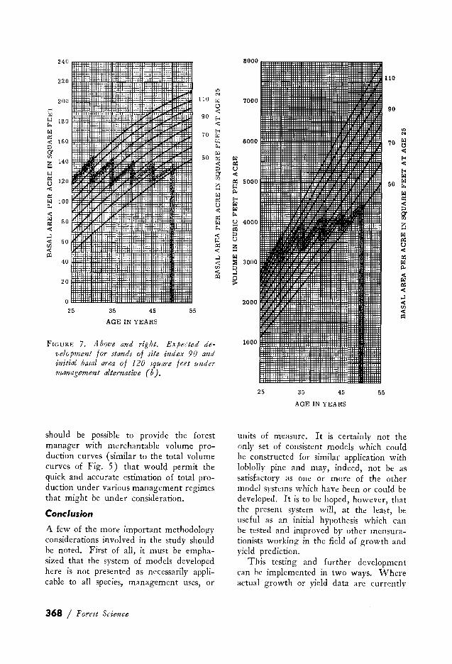
stand is 7,125 cubic feet. The develop­ment of stands receiving the management regime described in alternative (b) is shown in Figure 7. Table 4 presents the necessary computations for determining the total production under alternative (b). As indicated in Table 4, the estimated yields obtained under the thinning regime de­scribed in (b) are as shown in the tabula­tion at the right.

The cubic-foot volumes given above are total inside-bark volume including stump and top of all stems .5-inch dbh and above.

366 / Forest Science

Age

30 35 40 45 50

Total

Yield in wbic feet

500 625 525 425

4,450

6,525

If merchantable cubic-foot volume were used, the comparison would probably be considerably different. It is hoped that compatible models can be adapted for use with merchantable volume data. If so, it

TABLE 4. Computation of total stand production for stands of site index 90 and initial basal area of 120 square feet P·er acre under management alternative ( b).

Cut

2 3 4 5

Cutting age

Years

30 35 40 45 50

Basal area Initial density

class of Before cutting After cutting cut stand1

Square feet

141 120 100 141 120 80 137 120 64 135 120 53 134 0

Volume

Before cutting After cutting Yield

Cubic feet

3,575 3,075 500 3,925 3,300 625 4,075 3,550 525 4,225 3,800 425 4,450 0 4,450

6,525

'Initial density class of cut stand is defined as the stand basal area at age 25 which, on the same site index and in the absence of cutting, could be expected to produce a stand at the given cutting age with the specified basal area after cutting. These values are readily determined by reference to the basal area projection curves shown in Figure 7.

240

220 * 200 l!O

E-< r,:i 90 f.<l 180 r.. f.<l 70 a:: < 160 0 a C/l 50 2:: 140

f.<l a:: 120 u < a:: r,:i 100 ll,

< r,:i cc: 80 < ...:i < 60 C/l

< rll .':.t

40 + J i

20

0

25 35 45 55

AGE IN YEARS

F1GURE 6. Above and right. Expected devel­opment for stands of site index 90 and ini­tial basal area of 120 square feet under man­agement alternative (a).

8000

110

"' "' r,:i 7000 c.,

90 < E-< < E-< r,:i f.<l 6000 70 r.. r,:i i:i: r,:i < a:: 0 u a < C/l

:S a:: 5000 50 r,:i r,:i ll,

a:: E-< u r,:i < r,:i

a:: r.. r,:i u 4000 p. iii < 0 r,:i u o:;

~ < ...:i r,:i < ::;; 3000 C/l 0 < ...:i rll

~

2000

1000

25 35 45 55

AGE IN YEARS

volume 9, number 3, 19 63 / 367

240

220

"' "' 200 110 µ.l

c., E-o < µ.l 90 E-o µ.l 180

"" < E-o µ.l 70 a:: µ.l

< 160 µ.l ;:, "" a µ.l UJ 50 a:: ~

140 < ;:, µ.l a a:: 120 UJ u ~ <

µ.l a:: µ.l JOO a::

u p.. < < a:: µ.l

a:: 80 µ.l

< ~+ p..

...:i < µ.l < 60 a:: UJ

< < P'.l ...:i

40 < VJ

< 20

0

25 35 45 55

AGE IN YEARS

FIGURE 7. Above and right. Expe::ted de-velopment for stands of site index 90 and initial ba,·al area of 120 square feet under manageme,nt alternative ( b).

should be possible to provide the forest manager with merchantable volume pro­duction curves ( similar to the total volume curves of Fig. 5) that would permit the quick and accurate estimation of total pro­duction under various management regimes that might be under consideration.

Conclusion

A few of the more important methodology considerations involved in the study should be noted. First of all, it must be empha­sized that the system of models developed here is not presented as necessarily appli­cable to all species, management uses, or

368 / Forest Science

P'.l

8000

110

7000 90

"' "' r,;:i 6000 70 c., <

r,;:i E-o a:: < u E-o < r,;:i a:: 5000 50

r,;:i r,;:i "" p.. r,;:i E-o a:: r,;:i < r,;:i ::,

"" g u 4000

~ iii ::, r,;:i u a:: ::: u

< µ.l a:: ::;; 3000 r,;:i ::, p.. ...:i < ~ µ.l

a:: < ...:i

2000 < UJ < P'.l

1000

25 35 45 55

AGE IN YEARS

units of measure. It is certainly not the only set of consistent models which could he constructed for similar application with loblolly pine and may, indeed, not be as satisfactory as one or more of the other model systems which have been or could he developed. It is to be hoped, however, that the present system will, at the least, be useful as an initial hypothesis which can be tested and improved by other mensura­tionists working in the field of growth and yield prediction.

This testing and further development can he implemented in two ways. Where actual growth or yield data are currently

available, empirical tests can be made to check the validity of the actual equatio11s (if the available data are from loblolly pine stands of suitable description) or new equa­tions can be calculated to determine the applicability of the models to management systems other than that considered here. In the absence of actual data, model im­provement is still possible through a de­tailed consideration of the biological impli­cations that are inherent in the current sys­tem.

For example, the present models could be used to give answers to such questions as the following: ( 1) How is the density at which maximum growth occurs related to age and site? ( 2) Does the model allow for the possibility that, with sufficiently high density, net basal area or volume growth rates may become negative and, if so, what is the implied effect of site and age upon this density? ( 3) How is the rota­tion age of maximum mean annual incre­ment related to site, initial density, and thinning regime/

If the solutions provided to such ques­tions are internally contradictory or biologi­cally unreasonable, some revision of the model system is obviously necessary. It is of the utmost importance, however, to note that indicated revisions cannot generally be introduced into one portion of the system without affecting its logical compatibility with other components of the set. For ex­ample, any evidence refuting the form of the basal area growth model would almost certainly imply inaccuracy or inadequacy in the cubic-foot growth and yield models.

In view of the prevalence in the growth and yield literature of relative measures of density, some mensurationists will, no doubt, wish to consider and, perhaps, strictly adhere to models that avoid absolute meas­ures of stand density. It is, of course, im­possible to make general inferences, on the basis of this study, concerning the adequacy of possible compatible models systems which might use relative scales for the expression of stand density. However, it can be noted that the present system of models compares

favorably in predictive ability with the various southern pine growth or yield re­gressions that have used relative density measurements and for which some measure of predictive efficiency is available. In addi­tion, it is difficult to imagine the develop­ment of a complete model system with relative density expression that would not be considerably more complex conceptu­ally and analytically than the set of models developed here.

Finally, a comment may be pertinent as to the necessity for compatibility in growth and yield models for it may well be that many mensurationists will question wheth­er a search for consistency will justify the additional model construction and compu­tational effort that is necessary beyond that involved in the simple fitting of independ­ent growth and yield surfaces.

It would seem that at least two rather cogent arguments can be advanced to de­fend this additional labor. First, when growth and yield surfaces for the same stands are not compatible, at least one of them must be inadequate or inaccurate and the situation then certainly suggests that a gain in predictive efficiency can be realized by revising one or both of the models. Hence, when mensurationists propose non­compatible growth and yield models they are simultaneously presenting prim a f acie evidence that their predictors are not as good as they might be. Second, the briefest consideration of past and present scientific thought suggests that the development of logical but admittedly approximate relation­ships or predictors can be justifiably recog­nized as scientific achievements of compe­tence and importance.

However, it is difficult to point to any recognized contributions of importance or competence among such developments that involved the propounding of relationships that were, regardless of their predictive effi­ciency, obviously self-contradictory. One might speculate, for example, on the suc­cess which Newton might have achieved if he had attacked the problem of the pro­verbial aggressive apple by simply fitting

volume 9, number 3, 19 63 / 369

202 pp.

WAHLENBERG, W. G. 1960. Loblolly pine. Duke Univ. School Forestry, Durham, N. C. 603 pp.

WELLwoon, R. W. 1943. Trend towardo normality of stocking for second-growth

loblolly pine stands. J. For. 41 :202-209. WENGER, K. F., T. C. EvANs, T. LoTTI, R.

W. CooPER, and E. V. BRENDER. 1958. The relation of growth to stand density in natural loblolly pine stands. U. S. For­est Serv. Southeast. Forest Expt. Sta. Paper 97. 10 pp.

Commonwealth Forestry Bureau Oxford, England

Forestry Abstracts

This presents the essence of current world literature extracted by an experi­enced permanent staff from publications in over 30 languages (nearly 550 peri­odicals, 850 serials and innumerable miscellaneous papers, books, etc.) and now totalling over 5,500 abstracts each year. Special features include: the abstracting at length of literature published in the more unfamiliar languages ( e.g. Slav, Hun­garian and Oriental languages) ; notices of the more important critical reviews; notices of translations into English; notices of new journals and serials, or of changes in their style; and notices of atlases and maps. Each issue normally contains a leading article synthesizing authoritatively the literature on some par­ticular subject and also items of world news. Annual subscription is 110 s. or $16.50 U.S.A. or Canada, post-free.

Guide to the Use ol Forestry Abstracts

Containing a directory of publishing sources, analysis of an abstract notice, a key to abbreviations and many other aids, now available in an enlarged 4-language edition (English, French, German, Spanish) for 15s. or $2.25 post free, including five annual supplements.

Centralized Title Service

A quick-service postal auxiliary to the Abstracts bringing to subscribers four times a month exact copies of the index cards made from the world stream of forestry literature during the Bureau's day-to-day work, totalling about 7,000 annually. Full particulars and samples from: The Director, Commonwealth Forestry Bureau, Oxford.

Orders should be sent direct to: Central Sales Branch, Commonwealth Agricultural Bureaux,

Farnham Royal, Buckinghamshire, England

volume 9, number 3, 1963 / 371