118 IEEE TRANSACTIONS ON INSTRUMENTATION AND MEASUREMENT, VOL. IM-34, NO. 2, JUNE 1985

Accuracy of International Time and Frequency Comparisons Via Global Positioning System Satellites in

Common-View DAVID W. ALLAN, DICK D. DAVIS, SENIOR MEMBER, IEEE, M. WEISS, A. CLEMENTS, BERNARD GUINOT,

MICHEL GRANVEAUD, K. DORENWENDT, B. FISCHER, P. HETZEL, SHINKO AOKI, MASA-KATSU FUJJMOTO, L. CHARRON, AND N. ASHBY

Abstruct -Frequency differences between major national timing cen- ters are being resolved with uncertainty of less than 1 part in 1014;using satellites of the Global Positioning System (GPS) in common-view. Por- table clock and GPS time differences are in excellent agreement. Around the world GPS measurement between three laboratories had a time resid- ual of 5.1 ns.

I . INTRODUCTION MONG the units of the International System (SI) the A second, or its inverse the hertz, is unique in that local

time is the integral of the frequency generated by an SI stan- dard for the second. Because of this integral relationship, and taking advantage of the heterodyne principle wherein signifi- cant leverage is gained by measuring the frequency difference between two clocks, it is well known that one can measure the average frequency difference with arbitrary increasing accuracy simply by taking time difference readings between the two clocks over increasing integration time. A basic requirement is that the time instabilities of the measurement system be neg- ligibly small over the integration time. Over the history of com- parisons of international atomic frequency standards the time instabilities of the measurement systems have almost always been problematic and have clouded the comparisons. The ad- vent of the Global Positioning System (GPS) in common-view technique [ 11 has considerably reduced this problem. Insta- bilities of a few nanoseconds are now available internationally requiring integration times of only a few days in order to accu- rately measure the frequency difference between the best stan- dards in the world at the level of parts in

Manuscript received August 22,1984. D. W. Allan, D. D. Davis, M. Weiss, and A. Clements are with theTime

and Frequency Division, National Bureau of Standards, Boulder, CO 80303.

B. Guinot is with the Bureau International de l’Heure, 75014 Paris, France.

M . Granveaud is with the Laboratoire Primaire du Temps et des Fre- quences, 75104 Paris, France;

K. Dorenwendt, B. Fischer, and P. Hetzel are with the Physikalish- Technische Bundesanstalt, Bundesallee 100, D-3300 Braunschweig, Fed- eral Republic of Germany.

S. Aoki and M.-K. Fujimoto are with Tokyo Astronomical Obser- vatory, Mitaka, Tokyo 181, Japan.

L. Charron is with the Time Service Division, United States Naval Observatory, Washington, DC 20390.

N. Ashby is with the Department of Physics, University of Colorado, Boulder, CO 80309.

‘Note that the coordinate times are computed at the time of trans- mission, rather than at the times of reception as in this reference.

In summary, the common-view concept is as follows: if a transmitted event from a GPS satellite is viewed simultaneously from two sites, A and B , each maintaining an independent co- ordinate clock [2] , l then the coordinate times of the event can be computed at sites A and B as t & and t & B , respec- tively. If the true coordinate times of the transmitted event are tGA and t G B , respectively, then one can write the following:

~ G A = LA + ~ D A

~ G B = tbs + ~ D B

(1

(2 where the error terms tDA and tDB include errors in both mea- surement and calculation. These errors arise principally from errors in knowledge of the satellite position, and of the time delays in the propagation paths and receivers. The coordinate times of the transmitted event computed at sites A and B in- clude all known delay corrections such as the Sagnac correction [2] . Taking the difference between (1) and (2) yields an esti- mate of the true coordinate time difference between the A and B site clocks, ( t A - t B )

t A - t g = t i - tb + A t D

A t , = IDA - tDB

(3 1

(4)

where

and, where the difference, tL - t i , is the calculated value of the coordinate time difference.

Experimentally, it has been found that the size of the errors on the left side of (4) are about an order of magnitude smaller than those in either term on the right side, due to common- mode cancellation of errors. Hence, one sees the significant advantage of the simultaneous common-view approach. The residual RMS errors in A t D have been found to be of the order of 10 ns, and to have a white phase modulation spectrum [3] , [4]. The GPS common-view technique is about a factor of 20-30 times better than LORAN-C, for example, for averaging times of about 10 days.

The LORAN-C ground wave signal also has the disadvantage that it does not have global coverage; for high accuracy it is generally limited to North American and European compari- sons. In the past, integration times from a few months up to a year were necessary when using LORAN-C in order to conduct studies of clock instabilities between some of the best standards

U.S. Government work not protected by U.S. Copyright

ALLAN et al , : INTERNATIONAL TIME AND FREQUENCY COMPARISONS 119

in the world. Even then other issues tended to camouflage the sources of the instabilities being studied, such as annual varia- tions in the propagation delays or thermal coefficients in the clocks, along with other errors that sometimes accumulated in the delay paths.

Since GPS satellites orbit the earth with a 12-h period at about 4.2 Earth radii, and their orbits are inclined to the equator by 55-63", simultaneous common-view paths are readily avail- able for high latitude sites at reasonable elevation angles; the longitudes of two sites may be as much as 180" apart in a given hemisphere. Hence, global coverage is available using this tech- nique. Often more than one satellite may be observed in com- mon-view during one sidereal day. In addition, as the number of users increase the lengths of the baseline between adjacent user sites will decrease, thereby increasing the time and fre- quency accuracy and reducing the errors in (4). Thus as the system matures, the time and frequency transfer accuracy should increase.

If three or more satellites are available for observations be- tween two sites, one can estimate the frequency and timeinsta- bility of this measurement method, and instabilities of parts in 10'' have resulted for long integration times. The common- view technique also allows one to compare time readings accu- rately if the receiver delays have been calibrated. The estimated accuracy of this technique is about 10 ns, depending upon the baseline between the two receiver sites.

The GPS in common-view technique affords the first oppor- tunity to conduct an around-the-world Sagnac experiment with electromagnetic signals; in effect it is doing with microwave photons what Hafele and Keating did with portable atomic clocks several years ago [5] .

One of the principal benefits of the common-view technique is that it now allows meaningful comparisons between the pri- mary frequency standards throughout the world capable of generating the SI second. These comparisons can be made with a measurement uncertainty smaller than the uncertainty of the standards involved. Hence, the full accuracy of every primary frequency standard in the world in principle can be fully uti- lized in the generation of International Atomic Time (TAI).

Because the GPS is a military navigation system, and the possibility exists of encryption or degradation of the GPS sig- nals in the future, there is some concern about the long-term availability of the system for time and frequency comparisons. The simultaneous common-view technique may bypass in part, thanks to common-mode cancellations of errors, some of the problems that otherwise could arise.

11. THEORY OF COMMON-VIEW CLOCK COMPARISONS

In comparing time and frequency between two sites, any error in the GPS clock drops out in the subtraction, as has been shown in (1)-(3). However, ifthe common-view measurements are not exactly synchronous, some additional systematic errors can arise. These errors have not yet been well documented, but tend to be small. With asynchronism of the order of ten to twenty minutes, common-view errors have been observed to in- crease to as much as 20-30 ns. Errors of this type clearly will depend on the quality of the GPS clock and how well it and its space vehicle (SV) ephemeris are being modeled in the systems.

The time transfer error due to ephemeris errors-that is, due to uncertainties in satellite position-is one of the more signifi- cant error sources in the common-view technique. The error contributions of on-track, cross-track, and radial components of the vector position of the SV have been considered in detail in [ l ] and will be discussed later in this paper. Clearly, the shorter the baseline the smaller will be this contribution for a given satellite position error. Also, different components of position will contribute significantly different errors depending upon the satellite and site locations. The range of errors arising from ephemeris errors varies from about 2 to 50 ns depending upon the baseline between the two sites and its relationship to the satellite; typically the errors due to this source are less than 10 ns.

Uncertainties in propagation delays in the ionosphere and troposphere can also make a significant contribution to errors in the GPS common-view measurements. The model used in the GPS for ionospheric delay gives estimates whch are only accurate to about 50 percent [6 ] ; since the ionosphere can in- crease the propagation delay by several tens of nanoseconds this becomes an important concern. Fortunately, most of the precise timing centers are at fairly high latitudes where the ion- ospheric delay is significantly less than at the equator. Also, if the two sites are within one or two hour angles of each other there is some correlation in the ionosphere so that one achieves significant common-mode cancellation of ionospheric errors in the common-view approach [6] . For baselines and latitudes considered in this paper it is estimated that the common-view errors arising from this source are of the order of, or less than, 10 ns. If one chooses a nighttime propagation track, a separa- tion between sites of less than about two hours in angle and latitudes above 30", then common-mode cancellation reduces the ionospheric error to about 1 ns.

Since such conditions will be easier to achieve as more satel- lites are launched and more sites are available this error need not be a major problem. In principle one could measure the total electron content along the path using both of the available frequencies from the satellite, or by a Faraday rotation exper- iment. This adds significant complexity to the experiment and is not needed in order to reduce errors to less than 10 ns.

Reasonable models are built into the recievers for the tropo- sphere. These models can have large errors if significant water vapor variations occur over the tracking period. Typically, however, these only become significant if the elevation angles are very low. We have made an effort to keep all of the com- mon-view track angles above about 30" in order not to intro- duce significant error from tropospheric delay.

Since the PRN data rate for the GPS signal is 1.023 MHz it is necessary that the receiver circuitry be carefully conceived in order to realize 1 ns receiver delay stability and accuracy. In this regard it is also necessary that a reasonably large bandwidth is maintained at the receiver input, so that dependence on tem- perature and other effects do not cause long-term delay insta- bilities. Receiver delay stability of l ns has been demonstrated with current technology in some of the receivers utilized in the experiments reported here, by placing two totally independent receivers side by side. This produces cancellation of essentially all other effects except multipath distortion. Also in principle

120 IEEE TRANSACTIONS ON INSTRUMENTATION AND MEASUREMENT, VOL. IM-34, NO. 2 , J U N E 1985

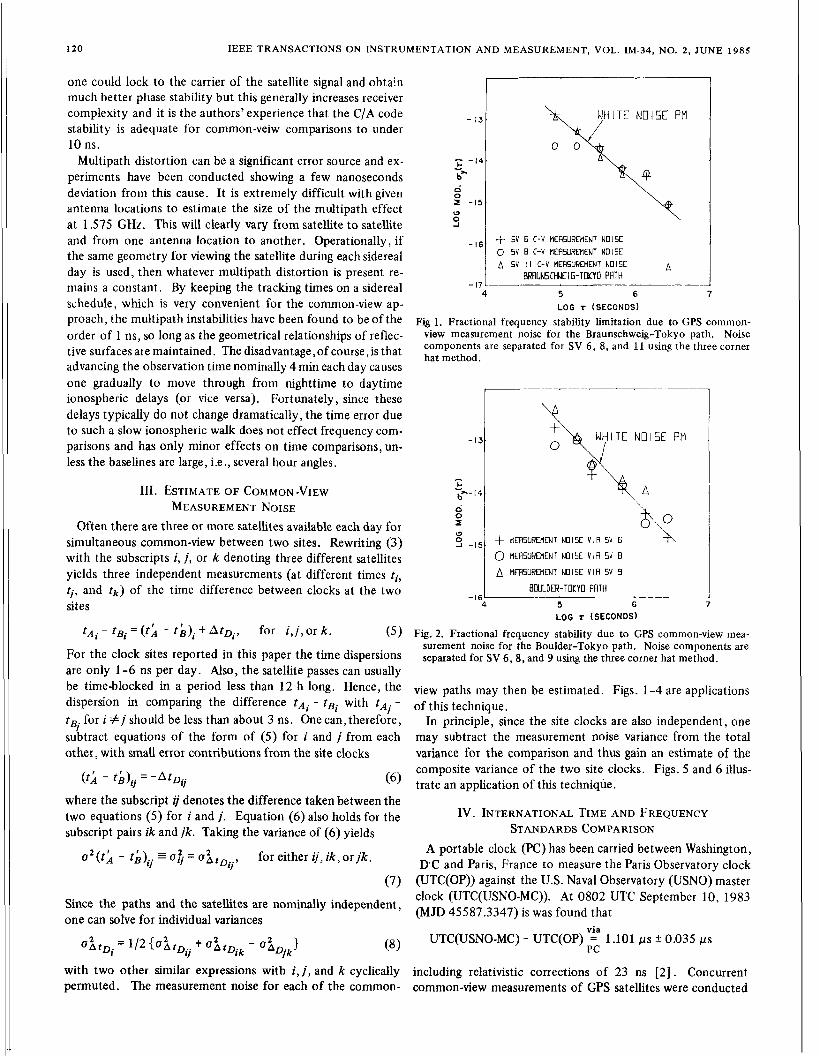
one could lock to the carrier of the satellite signal and obtain much better phase stability but this generally increases receiver complexity and it is the authors’ experience that the C/A code stability is adequate for common-veiw comparisons to under 10 ns.

Multipath distortion can be a significant error source and ex- periments have been conducted showing a few nanoseconds deviation from this cause. It is extremely difficult with given antenna locations to estimate the size of the multipath effect at 1.575 GH;!. This will clearly vary from satellite to satellite and from one antenna location to another. Operationally, if the same geometry for viewing the satellite during each sidereal day is used, then whatever multipath distortion is present re- mains a constant. By keeping the tracking times on a sidereal schedule, which is very convenient for the common-view ap- proach, the multipath instabilities have been found to be of the order of 1 ns, so long as the geometrical relationships of reflec- tive surfaces are maintained. The disadvantage, of course, is that advancing the observation time nominally 4 min each day causes one gradually to move through from nighttime to daytime ionospheric delays (or vice versa). Fortunately, since these delays typically do not change dramatically, the time error due to such a slow ionospheric walk does not effect frequency com- parisons and has only minor effects on time comparisons, un- less the baselines are large, i.e., several hour angles.

111. ESTIMATE OF COMMON-VIEW MEASUREMENT NOISE

Often there are three or more satellites available each day for simultaneous common-view between two sites. Rewriting (3) with the subscripts i, j, or k denoting three different satellites yields three independent measurements (at different times ti, ti, and t k ) of the time difference between clocks at the two sites

f A i - fBi = (tL - tb)i + A t D i , for i, j, or k. (5 J For the clock sites reported in this paper the time dispersions are only 1-6 ns per day. Also, the satellite passes can usually be time-blocked in a period less than 1 2 h long. Hence, the dispersion in comparing the difference tAi - tBi with t A . -

t for i # j should be less than about 3 ns. One can, therefore, Bi subtract equations of the form of (5) for i and j from each other, with small error contributions from the site clocks

I

( t i - t i ) . . 11 = -At, . . ‘1 ( 6 )

where the subscript z j denotes the difference taken between the two equations (5) for i and j . Equation ( 6 ) also holds for the subscript pairs ik and jk. Taking the variance of ( 6 ) yields

for either Q, ik, or jk. a 2 ( t i - th).. SE a$ = a i t o i j , 11

(7)

Since the paths and the satellites are nominally independent, one can solve for individual variances

‘ i t D i = 1 / 2 c a % t D . . + 11 ‘ a ’ D i k - ‘ADik 2 l (8 1 with two other similar expressions with i, j , and k cyclically permuted. The measurement noise for each of the common-

- 13

-14 - b” 0 0 Z -15 e 0 A

- I 6

- 17

H ITE NOI5E PM

-f SV 6 C-V IIERSUREHENT ND15E 0 SV B C-V flERSUREtIEN1 NOI5E A 5V II C-V tlER5UREHENT N015f

BRRUNSCHNEIE-TOKYO PRTH A

4 5 6 7 LOG T (SECONDS)

Fig 1. Fractional frequency stability limitation due to GPS common- view measurement noise for the Braunschweig-Tokyo path. Noise components are separated for SV 6 , 8, and 11 using the three corner hat method.

-f tlER5UREMENT NOISE V I R 5V 6 4\ 0

5 -15 0 IIEASUREMENT NOISE VIR SV B A MERSURMENT NOISE V I R 5V 9

BOULDER-TOKYO PRTH ._

4 5 6 LOG T (SECONDS)

Fig. 2. Fractional frequency stability due to GPS common-view mea- surement noise for the Boulder-Tokyo path. Noise components are separated for SV 6 , 8 , and 9 using the three corner hat method.

view paths may then be estimated. Figs. 1-4 are applications of this technique.

In principle, since the site clocks are also independent, one may subtract the measurement noise variance from the total variance for the comparison and thus gain an estimate of the composite variance of the two site clocks. Figs. 5 and 6 illus- trate an application of this technique.

Iv. INTERNATIONAL TIME AND FREQUENCY STANDARDS COMPARISON

A portable clock (PC) has been carried between Washington, D C and Paris, France to measure the Paris Observatory clock

(UTC(0P)) against the U.S. Naval Observatory (USNO) master clock (UTC(USN0-MC)). At 0 8 0 2 UTC September 10, 1983 (MJD 45587.3347) is was found that

UTC(USN0-MC) - UTC(0P) “5 1 . l o 1 ps k 0.035 ps PC

including relativistic corrections of 23 ns [2]. Concurrent common-view measurements of GPS satellites were conducted

ALLAN ef al. : INTERNATIONAL TIME AND FREQUENCY COMPARISONS 121

- I 2 L

-13

I b”-14

q I

? WHITE NUI5E PM

5 6 7 L O G T (SECONDS)

Fig. 3. Fractional frequency stability of GPS common-view measure- ments for the Boulder-Paris path via SV #9. Circles indicate com- posite noise of clocks and the SV #9 common-view link. Pluses are noise of the SV #9 link alone. Slope of white noise PM is shown for

-16 L

reference.

-I

- - 1

b” d 0 I 0 0

I

J -I<

WHITE NOISE PM I

- “4 5 6 L O G T (SECONDS)

Fig. 4. Fractional frequency stability of GPS common-view measure- ments for the Boulder-Braunschweig path via SV #9. Circles indicate composite noise of clocks and the SV #9 common-view link. Pluses are noise of the SV #9 link alone. Slope of white noise PM shown for reference .

-12

- -I?

b” d 0 I 0 ’ -14

-

-1s

I- PTE( C 5 I )-UTC( NE5) V I R 5V St E, 9

(CLOCK NOISE ONLY)

4 5 LOG T (SECONDS)

Fig. 5. Fractional frequency stability of GPS common-view measure- ments for the Boulder-Braunschweig path via SV numbers 5 , 8, and 9. (Common-view link noise removed.)

- 12

- -13

b” 0

c - 0 I 0 0

-14

-15

I __

5 6 L O G T (SECONDS)

Fig. 6. Fractional frequency stability of GPS common-view measure- ments for the Boulder-Tokyo path via SV numbers 6,8,and 9. (Com- mon-view link noise removed.)

between NBS Boulder and USNO, and between NBS Boulder and OP, using (electromagnetic) signals from GPS satellites to derive time comparisons. The Sagnac correction from Boulder, CO, to Paris, France, varies from 71 to 1 12 ns and from Boulder to Washington, DC, varies from 11 to 13 ns, depending on satel- lite position. Using the appropriate relativistic corrections for each common-view time difference obtained via GPS NAVSTAR 4 , 5 , and 6 satellites, yields

UTC(USN0-MC) - UTC(0P) “f 1.100 ps f 0.02 ps GPS

in excellent agreement with the portable clock trip. More recently (April 18, 1984, MJD 45808.248), two PC’s

were carried between Physikalisch-Technische Bundesanstalt (PTB) and OP. The weighted combination of the comparisons using PC’s gave the result

UTC(PTB) - UTC(0P) vc - 1.070 ps k 0.020 ps. PC

At the same date the GPS common-view technique gave the result

UTC(PTB) - UTC(0P) 2” -1.090 ps f 0.010 ps. GPS

Agreement between the two methods of comparison of coordi- nate clocks is within the combined measurement uncertainties, and is evidence that a coordinate time clock network can be established near the earth for which synchronization using por- table clocks or electromagnetic signals agree.

The primary standards at PTB [7] and NBS [8] are now being compared using the GPS in common-view method with an estimated precision of measurement of less than 1 part in 1014. During July 1983 NBS performed an evaluation of its primary frequency standard NBS-6. This evaluation is con- ducted anpually to provide data to the Bureau International de 1’Heure (BIH) for the calibration of the rate of TAI. The evaluation included the recently discovered black body radia- tion frequency shift correction [9] . GPS common-view mea- surements between PTB and NBS also began in July of 1983,

122

- I

c t- - b” d 0 z a 4

-I

IEEE TRANSACTIONS ON INSTRUMENTATION AND MEASUREMENT, VOL. IM-34, NO. 2, JUNE 1985

T

t UTC(U5NO-nO-P16(CSI) VIfl 5V I I tlJD ’KT20 - 4S787 RfBN IDIF 0.107978 Et02 RnVD

~. - ~

5 6 7 LOG T (SECONDS)

Fig. 7. Fractional frequency stability of UTC(USN0-MC) - PTB(CS1) via GPS SV 11, common-view measurements for the Washington- Braunschweig path. The mean normalized frequency difference over this interval was 1.25 X

and the frequency of the PTB primary frequency standard CS1 was measured versus UTC(NBS) via space vehicles 5, 8 , and 9 providing three independent comparisons. The GPS measure- ments were averaged over twenty days; the standard deviation of the mean was 4 parts in The accuracy of the NBS-6 calibration was 9 parts in l O I 4 and the accuracy of the PTB CS1 measurement was 2 parts in In the following equa- tions, which list the measured and calculated results, y denotes tions, which lists the measured and calculated results, y denotes ments, @ g.r. denotes the geoid in rotation, (i.e.,mean sea level) the asterisk means the results are not corrected for black-body radiation shift, and the uncertainty is that for PTB CSl .

YUTC(NBS) - y ~ ~ s - 6 = (-1.8 k 0.9) x w3. (9)

The differences

Y c s i * @ g.r. - YUTC(NBS) = (0.18 * 0.04) X (IO)

are measured via GPS satellite vehicles numbers 5, 8 , and 9. Also,

YNBS-6 -YNBS-6 @ g.r. = 1.8 x Y c s i * @ g.r. - Ycsl e g.r. = (-0.17 f 0.2) X

(11)

(12)

Combining (9)-(12) yields

YCSl @ g.r. - YNBs-6 @ g.r. = (0.35 * 0.92) (13)

For 280 days from July 1983 (MJD 45522), the frequency and frequency stability of the USNO master clock, UfC(USN0- MC), was measured against the PTB CS1 primary frequency standard using GPS in common-view. A plot of the fractional frequency stability is shown in Fig. 7.

Beginning August 1982, Tokyo Astronomical Observatory (TAO) GPS data as well as its LORAN-C measurements became available on the General Electric Mark 111 computer network. The USNO began using this GPS data to supplement the time transfers obtained via the Defense Satellite Communication System and portable clock measurements to calibrate and deter- mine better values of UTC(USN0-MC) minus LORAN-C in the northwest Pacific [ l o ] , [ I 11.

Fig. 8 illustrates the differences between UTC(USN0-MC) and UTC(TA0). The square symbols indicate differences deter- mined using the common-view data for SV6. The line of data points passing through these GPS values is obtained using the LORAN-C averaged time scale which is available 7-10 days in arrears. Using the values from USNO Series 4 which is pub- lished daily in a teletype message, one can see some oscilla- tions about the time scale determinations. While a difference of approximately 0.5 ps may be seen at about MJD 45650, the agreement is generally much better than 0.5 ps. The scatter seen is due to the incomplete data that must be used to pro- vide “real-time” differences for publication, and to quantiza- tion errors. A portable clock measurement is indicated by the arrow.

It should be noted that individual systematic corrections are applied by USNO to the LORAN-C measurements received so that data from many stations can be used in the formation of a time scale for a remote site. These systematic corrections are required to provide a mutually self-consistent system [ 121 . Figs. 9 and 10 are plots of UTC(USN0-MC) minus UTC(0P) and UTC(USN0-MC) minus UTC(PTB), respectively. The con- tinuous curve represents those values obtained via GPS SV6. The second indicates values one obtains using the Series 4 data. A systematic correction of 0.63 ps has been applied to the PTB LORAN-C data while a correction of 0.87 ps has been applied to the OP data.

One may note a step‘of approximately 0.6 p s at MJD45731 appearing in both Figs. 9 and 10. T h s is an artifact introduced when data from the Labrador Sea LORAN-C chain entered into the equations used to determine values for the Norwegian Sea chain. The exact location of the error is not yet known. A USNO project to calibrate the time of emission of each LORAN-C chain and the total system delay of major monitor- ing sites is presently planned. If a rate offset and time offset are subtracted from the data in Fig. 10, a comparison of the relative stabilities of the two techniques is obtained (see Fig. 11).

V. SAGNAC EXPERIMENT Using the timing centers (NBS) in Boulder, CO, (PTB) in

Braunschweig, Germany and (TAO) in Tokyo, Japan, the time differences were measured using the GPS in common-view tech- nique for the months of April, May, and June 1984. Using three satellites for each of the three common-view paths, we estimated the measurements noise and the optimum weighting factor. Knowing these parameters, we obtained an optimum Kalman-smoothed estimate of the time and frequency differ- ence between each of the three timing centers. The following are the mean time and mean frequencies for this globeencircling Sagnac experiment:

3 .I? Lab pair X

UTC(PTB)- UTC(NBS) -5383.8 ns -1.313 X UTC(TA0) - UTC(PTB) t2598.0 ns t0.658 X UTC(NBS) - UTC(TA0) t2791 .O ns t0.639 X

= t 5 .2 ns -0.016 X

ALLAN et aL: INTERNATIONAL TIME AND FREQUENCY COMPARISONS

3.0

2 . 6

2.G

2.4

2.2

2.0

1.6

1 . G

1.4

1.2

PS 1.0

0.e

0.G

0.11

0.2

-0.0

-0.2

-0.4

-0.G

-0.8

-1.0

Fig. 8. Values of UTC(USNQMC) minus UTC(TA0) by three methods. The square symbols are data obtained using the GPS common-view technique with SV #6. The small dots are obtained using data as published for LORAN€ in TSA Series 4. The line of data points lying on top of the GPS data are comparisons using LORAN€ as a time scale, [ 111. Note the good agreement with the portable clock measurement indicated by the arrow.

1.6

1:: j 1.0

0.8

0.6

0.u

0.2

/Js -0.0

-0.2

-0.9

-0.6

-0.8

-1.0

-1.2

1::: 1 -1.8 f

1983 198U Fig. 9. Values of UTC(USNO-MC) minus (UTC(0P) by two methods. The line of data points is obtained using GPS SV #6

in common-view. The dots are obtained via LORAN4 as published in TSA Series 4. A PC Measurement is indicated by the arrow.

123

124 IEEE TRANSACTIONS ON INSTRUMENTATION AND MEASUREMENT, VOL. IM-34, NO. 2, JUNE 1985

4.0

3 . 6

3. G

3.11

3.2

3.0

2.8

2.6

2.q

2.2

2.0

1.6

D.Is I . G

1.4

1.2

-1.0 1 I I 1 I , I I , 1 I ' I I , I I u55" U 5 6 M us usm ' u I I ,v&I I I : I ,

SEPT OCT I x l V OEC JRN FEE MARCH RPAIL MRY JUNE

1983 198q Fig. 10. Values of UTC(USN0-MC) minus UTC(PTB) by two methods.

The line of data points is obtained using GPS SV #6 incommon-view. The dots are obtained via LORAN€ as published in TSA Series 4. A PC measurement is indicated by the arrow.

UTC(USNO)-UTC(PTB) nr .

0

-400 .

-800 '

-1200

-1600

i, x vIn cps

4SS80 45620 4S6S0 45700 45740 457B0 45820 4SB6E MJD

Fig. 11. Values of UTC(USN0-MC) minus UTC(PTB) derived from data in Fig. 10 by application of rate and time offset connections.

where 2 denotes the estimate of the average time difference and 3 denotes the estimate of the normalized average frequency difference over the three months. The total magnitude of the Sagnac correction varies from about 230 to 350 ns depending upon which satellites are employed. Since the Sagnac effect is accounted for in the software of each receiver the residuals should add to zero. The frequency residuals are about an order of magnitude better than the clocks involved. The net result of the experiment is that we have validated the around-the- world Sagnac effect with an uncertainty which is about 2 per- cent of the total effect.

VI. CONCLUSIONS International time and frequency comparisons are operation-

ally possible at state-of-the-art levels of accuracy using GPS satellites in common-view of two Earth timing centers. Inte- gration times of about four days and longer are sufficient to

ALLAN et al. : INTERNATIONAL TIME AND FREQUENCY COMPARISONS 125

measure the time differences between major international tim- ing centers to an accuracy of about 10 ns. The accuracy of international frequency comparisons is a function of the inte- gration time and is given approximately by 4 X T-’”,

where T is in days and the frequency is a normalized frequency. The quantity T ranges from one day to about a month. This technique affords the first opportunity to compare atomic clocks internationally on an operational basis, with measure- ment instabilities smaller than the clockinstabilities. This tech- nique is about 10-100 times better than the LORAN-C ground wave technique; in addition it has worldwide coverage.

The common-view technique requires the comparison data from two or more sites. This is accomplished for the major timing centers using the international General Electric Mark I11 computer system. Common telephone modems with automatic dialers have been utilized for this purpose and work well for North American and European comparisons. A data format has been agreed upon and a set of class bytes designating compari- sons with different areas of the globe has been constructed. Any of the authors can be contacted for access to these, and NBS is currently coordinating the class byte and track time values.

Though the GPS is a military navigation system, there are good indications that it will be available to the civilian com- munity for many years to come. It is anticipated that the em- ployment of this GPS common-view technique will significantly improve both the performance and comparison of national and international time scales.

ACKNOWLEDGMENT

The authors wish to acknowledge the suggestions of Dr. Gernot M. R. Winkler and Dr. David J. Wineland as readers of this DaDer. In addition sienificant contributions were made by

staff members (too many to enumerate) of the org.r*iizations involved for which the authors are deeply appreci c t’ 1vt.

REFERENCES D. W. Allan and M. A. Weiss, “Accurate time and frequency trans- fer during common-view of a GPS satellite,” in Roc . 34th Ann. Freq. Contr. Symp., May 1980. N. Ashby and D. W. Allan, “Practical implications of relativity for a global coordinate time scale,” in Roc. URSZSymp. on Time and Freq. 1978; Also, Radio Sci., vol. 14, p. 649,1979. D. D. Davis, M. A. Weiss, A. C. elements, and D. W. Allan, “Con- struction and performance characteristics of a prototype NBS/ GPS receiver,” in Proc. 35th Ann. Symp. on Frequency Control, pp. 546-552, May 27-29,1981. D. D. Davis, M. A. Weiss, A. C. elements, and D. W. Allan, “Re- mote synchronization within a few nanoseconds by simultaneous viewing of the 1.575 GHz GPS satellite signals,”ConJ onfiecision Electromagnetic Meas. Digest., Cat. 82CH17376, PN-15,1982. J . C. Hafele and R. E. Keating, “Around-the-world atomic clocks: Observed relativisitic time gains,” Science, vol. 177, pp. 168-170, July 1972. J. A. Klobluchar, “Ionospheric effects on satellite navigation and air traffic control systems,” in NATO AGARD Proc., Lecture Ser. no. 93, Recent Advances in Radio and Optical Propagation for Modern Communication, Navigation, and Detection Systems, 1978. G. Becker, “Performance of the primary Cs-standard of the Phys- ikalick-Technische Bundesanstalt,” Metrologia, vol. 13, pp. 99- 104,1977. D. J . Wineland, D. W. Allan, D. J. Glaze, H. W. Hellwig, and S. Jarvis, Jr., “Results on limitations in primary cesium standard operation,” IEEE. nuns. Instrum. Meas., vol. IM-25, p. 453, 1976. W. M. Itano, L. L. Lewis, and D. J . Wineland, Phys. Rev., vol. 425, p. 1233,1982. L. G. Charron, “Relationships between U.S. Naval Observatory, Loran-C, and defense satellite communications system ,” in Proc. of the 13th Precise Time and Time Interval (PTTI) Appl. and Planning Meeting, Washington, DC, Dec. 1981. C. F. Lukac and L. G. Charron, “Timing a Loran-C chain,” Nav. J. of the Znst. of Nav., vol. 29, no. 3, Fall, 1982, Washington, DC. L. G. Charron and C. F. Lukac, “Evolution of Loran-C timing technique,” to be published.