Imperial College London

Department of Computing

Comparison of Training Methods for

Deep Neural Networks

Patrick Oliver GLAUNER

April 2015

Supervised by Professor Maja PANTIC

and Dr. Stavros PETRIDIS

Submitted in part fulfilment of the requirements for the degree of

Master of Science in Computing (Machine Learning) of Imperial College

London

1

arX

iv:1

504.

0682

5v1

[cs

.LG

] 2

6 A

pr 2

015

Declaration

I herewith certify that all material in this report which is not my own work has

been properly acknowledged.

Patrick Oliver GLAUNER

2

Abstract

This report describes the difficulties of training neural networks and in particu-

lar deep neural networks. It then provides a literature review of training meth-

ods for deep neural networks, with a focus on pre-training. It focuses on Deep

Belief Networks composed of Restricted Boltzmann Machines and Stacked Au-

toencoders and provides an outreach on further and alternative approaches. It

also includes related practical recommendations from the literature on training

them. In the second part, initial experiments using some of the covered meth-

ods are performed on two databases. In particular, experiments are performed

on the MNIST hand-written digit dataset and on facial emotion data from a

Kaggle competition. The results are discussed in the context of results reported

in other research papers. An error rate lower than the best contribution to the

Kaggle competition is achieved using an optimized Stacked Autoencoder.

3

Contents

1 Introduction 8

2 Neural networks 10

2.1 Feed-forward neural networks . . . . . . . . . . . . . . . . . . . . 10

2.2 Other types of neural networks . . . . . . . . . . . . . . . . . . . 12

2.3 Training neural networks . . . . . . . . . . . . . . . . . . . . . . . 14

2.3.1 Difficulty of training neural networks . . . . . . . . . . . . 15

2.4 Regularization . . . . . . . . . . . . . . . . . . . . . . . . . . . . 16

2.4.1 L2 and L1 regularization . . . . . . . . . . . . . . . . . . . 16

2.4.2 Early stopping . . . . . . . . . . . . . . . . . . . . . . . . 17

2.4.3 Invariance . . . . . . . . . . . . . . . . . . . . . . . . . . . 18

2.4.4 Dropout . . . . . . . . . . . . . . . . . . . . . . . . . . . . 18

3 Deep neural networks 20

3.1 Restricted Boltzmann machines . . . . . . . . . . . . . . . . . . . 20

3.1.1 Training . . . . . . . . . . . . . . . . . . . . . . . . . . . . 23

3.1.2 Contrastive divergence . . . . . . . . . . . . . . . . . . . . 23

3.2 Autoencoders . . . . . . . . . . . . . . . . . . . . . . . . . . . . . 24

3.2.1 Sparse autoencoders . . . . . . . . . . . . . . . . . . . . . 25

3.2.2 Denoising autoencoders . . . . . . . . . . . . . . . . . . . 26

3.3 Comparison of RBMs and autoencoders . . . . . . . . . . . . . . 26

3.4 Deep belief networks . . . . . . . . . . . . . . . . . . . . . . . . . 27

3.4.1 Stacked autoencoders . . . . . . . . . . . . . . . . . . . . 29

3.5 Further approaches . . . . . . . . . . . . . . . . . . . . . . . . . . 29

3.5.1 Discriminative pre-training . . . . . . . . . . . . . . . . . 30

3.5.2 Hessian-free optimization and sparse initialization . . . . 30

4

3.5.3 Reducing internal covariance shift . . . . . . . . . . . . . 30

4 Practical recommendations 32

4.1 Activation functions . . . . . . . . . . . . . . . . . . . . . . . . . 32

4.2 Architectures . . . . . . . . . . . . . . . . . . . . . . . . . . . . . 33

4.3 Training of RBMs and autoencoders . . . . . . . . . . . . . . . . 34

4.3.1 Variations of gradient descent in RBMs . . . . . . . . . . 34

4.3.2 Autoencoders . . . . . . . . . . . . . . . . . . . . . . . . . 37

4.3.3 Fine-tuning of DBNs . . . . . . . . . . . . . . . . . . . . . 38

5 Application to computer vision problems 39

5.1 Available databases . . . . . . . . . . . . . . . . . . . . . . . . . . 39

5.1.1 MNIST . . . . . . . . . . . . . . . . . . . . . . . . . . . . 39

5.1.2 Kaggle facial emotion data . . . . . . . . . . . . . . . . . 40

5.2 Available libraries . . . . . . . . . . . . . . . . . . . . . . . . . . 41

5.2.1 Hinton library . . . . . . . . . . . . . . . . . . . . . . . . 41

5.2.2 Deep Learning Toolbox . . . . . . . . . . . . . . . . . . . 41

5.3 Experiments . . . . . . . . . . . . . . . . . . . . . . . . . . . . . . 42

5.3.1 Classification of MNIST . . . . . . . . . . . . . . . . . . . 42

5.3.2 Classification of Kaggle facial emotion data . . . . . . . . 44

6 Conclusions and prospects 49

Bibliography 51

5

List of Tables

5.1 Model selection values for MNIST . . . . . . . . . . . . . . . . . 42

5.2 Model selection for DBN and SAE on MNIST, lowest error rates

in bold . . . . . . . . . . . . . . . . . . . . . . . . . . . . . . . . . 44

5.3 Error rates for optimized DBN and SAE on MNIST, lowest error

rate in bold . . . . . . . . . . . . . . . . . . . . . . . . . . . . . . 44

5.4 Model selection values for Kaggle data . . . . . . . . . . . . . . . 45

5.5 Model selection for DBN and SAE on Kaggle data, lowest error

rates in bold . . . . . . . . . . . . . . . . . . . . . . . . . . . . . 47

5.6 Error rates for optimized DBN and SAE on Kaggle data, lowest

error rate in bold . . . . . . . . . . . . . . . . . . . . . . . . . . . 47

6

List of Figures

2.1 Neural network with two input and output units and one hidden

layer with two units and bias units x0 and z0 [8] . . . . . . . . . 11

2.2 History of neural networks [28] . . . . . . . . . . . . . . . . . . . 13

2.3 L1 and L2 regularization [34] . . . . . . . . . . . . . . . . . . . . 17

2.4 Left: a neural network with two hidden layers. Right: a result

of applying dropout to the same neural network. . . . . . . . . . 18

3.1 Restricted Boltzmann Machine with three visible units and two

hidden units (and biases) . . . . . . . . . . . . . . . . . . . . . . 21

3.2 Autoencoder with three input and output units and two hidden

units . . . . . . . . . . . . . . . . . . . . . . . . . . . . . . . . . . 24

3.3 Deep belief network structure . . . . . . . . . . . . . . . . . . . . 28

3.4 Deep belief network layers learning complex feature hierarchies

[41] . . . . . . . . . . . . . . . . . . . . . . . . . . . . . . . . . . . 29

4.1 Features learned by 100 hidden units of the same layer [6] . . . . 38

5.1 Hand-written digit recognition learned by a convolutional neural

network [47] . . . . . . . . . . . . . . . . . . . . . . . . . . . . . . 40

5.2 Sample data of the Kaggle competition [26] . . . . . . . . . . . . 41

5.3 Test error for different L2 regularization values for training of DBN 43

5.4 Test error for different learning rates values for training of DBN . 46

7

1 Introduction

Neural networks have a long history in machine learning. Early experiments

have shown both, their expressional power, but also the difficulty to train them.

For the last ten years, neural networks are celebrating a comeback under the

label ”deep learning”. Enormous efforts in research have been made on this

topic, which attracted major IT companies including Google, Facebook, Mi-

crosoft and Baidu to make significant investments in deep learning.

Deep learning is not simply a revival of an old theory, but it comes with

completely different ways of building and training many-layer neural networks.

This rise has been supported by recent advances in computer engineering, in

particular the strong parallelism in CPUs and GPUs.

Most prominently, the so-called ”Google Brain project” has been in the news

for its capability to self-learn cat faces from images extracted from YouTube

videos as presented in [35]. Aside from computer vision, major advances in

machine learning have been reported in audio and natural language processing.

These advances have been raising many hopes about the future of machine

learning, in particular to work towards building a system that implements the

single learning hypothesis as presented by Ng in [2].

Nonetheless, deep learning has not been reported to be a easy and quick to use

silver bullet to any machine learning problem. In order to apply the theoretical

foundations of deep learning to concrete problems, much experimentation is

required.

Given the success reported in many applications, deep learning looks prom-

ising to be applied to various computer vision problems, such as hand-written

digit recognition and facial expression recognition. For the latter, only few

results have been reported so far, such as in [29] and [33], and to intelligent

behavior understanding as whole. An example is the work in [45], which won

8

the 2013 Kaggle facial expression competition [26] using a deep convolutional

neural network.

9

2 Neural networks

This chapter provides a summary of neural networks, their history and train-

ing challenges. Prior exposure to neural networks is assumed, this chapter is

therefore not considered to give an introduction to neural networks.

The perceptron introduced by Rosenblatt in 1962 [15] is a linear, non-dif-

ferentiable classifier, making it of very limited use on real data. Quite related

to perceptrons, logistic regression is a linear classifier, whose cost function is

differentiable. Inspired by the brain, neural networks are composed of layers of

perceptrons or logistic regression units.

2.1 Feed-forward neural networks

In their simplest form, feed-forward neural networks propagate inputs through

the network to make a prediction, whose output is either continuous or dis-

crete, for regression or classification, respectively. A simple neural network is

visualized in Figure 2.1.

Using learned weights Θ, the activation of unit i of layer j + 1 can be calcu-

lated:

a(j+1)i = g

( sj∑k=0

Θ(j)ik xk

)(2.1)

g is an activation function. Most commonly, the Sigmoid activation function1

1+e−x is used for classification problems.

Given the limitations of a single perceptron unit, [30] led to a long-standing

debate of perceptrons and to a misinterpretation of the power of neural net-

works. As a consequence, research interest and funding in research on neural

networks dropped for about two decades.

10

Figure 2.1: Neural network with two input and output units and one hiddenlayer with two units and bias units x0 and z0 [8]

Another downside of neural networks is learning the weights between the

large amounts of parameters and the required computational resources, which

is covered in Chapter 2.3. In the 1980s, regained attention in research led to

backpropagation, an efficient training algorithm for neural networks.

Subsequent research led to very successful applications, such as the following

examples. The Mixed National Institute of Standards and Technology (MNIST)

database [49] is a large collection of handwritten digits with different levels of

noise and distortions. Classifying handwritten digits is needed in different tasks,

for example in modern and highly automated mail delivery. Neural networks

were found in the 1980s to perform very well on this task. Autonomous driving

is subject to current research in AI. Back in the 1980s, significant steps in this

field were made using neural networks as shown by Pomerleau in [10].

Neural networks are known to learn complex non-linear hypotheses very

well, leading to low training errors. Nonetheless, training a neural network

is non-trivial. Given properly extracted features as input, most classification

problems can be done with one hidden layer quite accurately as described in

[25]. Adding another layer allows to learn even more complex hypotheses for

11

scattered classes. There are many different (and contradictory) approaches to

finding appropriate network architectures as summarized and discussed in [40].

In general, the more units and layers, the higher a network’s expressional power.

This makes training more difficult.

Extracting proper features is a major difficulty in signal processing and com-

puter vision as presented by Ng in [2]. Neural networks with many hidden

layers allow to learn features from a dataset themselves, coming with enormous

simplifications in those fields. The computational expensiveness and the low

generalization capabilities of deep neural networks resulted in another decline

of neural networks in the 1990s as described in [28].

Many-layer neural networks, so-called deep neural networks, have been re-

ceiving lots of attention for about the last ten years because of new training

methods, which are covered in Chapter 3. These developments have achieved

significant progress in machine learning, as described in Chapter 1 and in [18],

[20] and [27]. In addition to new training methods, advances in computer en-

gineering, in particular faster CPUs and GPUs, have supported the rise of deep

neural networks. GPUs have proved to significantly speed up training of deep

neural networks, as reported in [1]. This has also been raising many hopes

about the future of machine learning to push its frontiers towards building a

system that implements the single learning hypothesis as presented by Ng in

[2].

As visualized in Figure 2.2, the history of neural networks can be plotted

on a hype curve with open questions and resulting uncertainty of the future of

neural networks.

2.2 Other types of neural networks

In addition to feed-forward networks, there are two other popular types of

neural networks: convolutional and recurrent neural networks [8]. Convo-

lutional neural networks (CNN) are a special kind of feed-forward networks

that include invariance properties in their architecture, for example to tolerate

translation of the input. Their structure implies constraints on the weights,

as weights are shared within so-called feature maps. This approach reduces

12

Figure 2.2: History of neural networks [28]

the number of independent parameters and therefore speeds up learning using

minor modifications in backpropagation. CNNs have been used successfully in

computer vision, for example on MNIST. Recurrent neural networks (RNNs)

are cyclic graphs of units. This architecture results in an internal state of the

network, allowing it to exhibit dynamic temporal behavior. In practice, train-

ing RNNs can come with complex graph problems, making them difficult to

understand and train reliably.

Stochastic neural networks covered in [14] are special type of neural networks.

They include random variations in either their weights or in their activation

function. They allow to escape from local optima. Boltzmann Machines and

Restricted Boltzmann Machines presented in Chapter 3 are stochastic neural

networks.

13

2.3 Training neural networks

In order to train a neural network, its prediction error is measured using a cost

function, for which there are many different ones in the literature, such as least

squares cost function

J(Θ) =

m∑i=1

(y(i) − hΘ(x(i)))2 (2.2)

and cross-entropy cost function covered in [42], which is meant to generalize

better and speed up learning as discussed in [4]:

J(Θ) = −

(m∑i=1

y(i) log hΘ(x(i)) + (1− y(i)) log(1− hΘ(x(i)))

)(2.3)

Cost functions of neural networks are highly non-convex as visualized by Ng

in [4]. Therefore, finding the global minimum of the cost function is difficult

and optimization often converges in a local minimum.

In order to minimize the error function, the partial derivatives of the network

parameters are calculated: The simplest method to approximate the gradient

of any cost function is to utilize finite differences:

∂

∂θiJ(θ) ≈ J(..., θi−1, θi + ε, θi+1, ...)− J(θ)

ε(2.4)

Alternatively, symmetric differences allow higher precision:

∂

∂θiJ(θ) ≈ J(..., θi−1, θi + ε, θi+1, ...)− J(..., θi−1, θi − ε, θi+1, ...)

2ε(2.5)

Both methods are computationally inefficient, as the cost function needs to

be evaluated twice per partial derivative. In the 1980s, backpropagation was

developed, which is an efficient method to compute the partial derivatives [42].

Its main idea is to start with random initial weights between the units and then

to propagate training data through the network. Initial weights are random,

in order to avoid symmetrical behavior of the neurons that would lead to an

inefficient and redundant network behavior. The magnitude of error is then

14

used to layer-wise backpropagate derivatives of the error, which are finally used

to update the weights. This leads to a reduction of the training error.

Next, the partial derivatives are used in an optimization algorithm to min-

imize the cost function, such as in gradient descent defined in Algorithm 2.1.

Each update of gradient descent goes through the entire training set of m train-

ing examples, making single updates expensive. Furthermore, gradient descent

does not allow to escape local minima, as each update steps goes further down

the cost function towards a minimum.

Algorithm 2.1 Batch gradient descent: training size m, learning rate α

repeatθj ← θj − α ∂

∂θjJ(θ) (simultaneously for all j)

until convergence

In practice, preferably stochastic gradient descent, also named online gradient

descent, defined in Algorithm 2.2 is used in neural networks, as explained by

LeCun in [48]. It wanders around minima and lacks certain convergence criteria

of gradient descent. For example, some update steps might go away from the

nearest minimum or even up on the cost function. In contrast, each update step

is for a single training example, making updates much faster. Also, stochastic

gradient descent allows to escape local minima under certain circumstances.

Algorithm 2.2 Stochastic gradient descent: training size m, learning rate α

Randomly shuffle data setrepeat

for i = 1 to m doθj ← θj − α ∂

∂θjJ(θ, (x(i), y(i))) (simultaneously for all j)

end foruntil convergence

2.3.1 Difficulty of training neural networks

In general, the more units and layers, the higher a network’s expressional power.

This comes with a more complex cost function. Learning will then easily get

stuck in a local minimum, leading to high generalization errors and overfitting.

15

There are different methods to reduce overfitting, for example smaller networks,

more training data, better optimization algorithms, or regularization, which is

covered in Chapter 2.4.

Deep learning utilizes deep neural networks consisting of many layers of neur-

ons. In principle, backpropgation works on such networks as well. Nonethe-

less, it does not perform very well on large networks because of the following

considerations: For small initial weights, the partial derivative updates back

propagated through many layers will be very small or 0 because of numerical

effects, leading to very unsatisfiable updates. This is also known as the vanish-

ing gradient problem. On the other hand, large initial weights will make the

training get stuck from the beginning on in some region of the cost function, not

allowing to converge to the global or better local minimum, which is covered in

detail in [11] and [12].

2.4 Regularization

Regularization allows to reduce overfitting of neural networks and learning al-

gorithms in general. This section covers different regularization methods.

2.4.1 L2 and L1 regularization

Large parameter values often allow models to match training data well, but do

not generalize to new data. L2 and L1 regularization ”penalize” large parameter

values, by adding them to the cost function.

For the weights, the following notation of Ng in [5] is used: Θ(l) is a matrix

of weights to map from layer l to layer l+1. If the network has sl units in layer

l and sl+1 units in layer l + 1, then Θ(l) is of dimension sl+1 × (sl + 1), also

considering the extra bias unit.

L2 regularization also known as weight decay is used predominantly and adds

the squared weights to the cost function:

Jreg(Θ) = J(Θ) + λ

L−1∑l=1

sl+1∑i=1

sl∑j=1

(Θ

(l)ij

)2(2.6)

16

The magnitude of the regularization can be controlled by the regularization

parameter λ, whose value is often subject to model selection.

An alternative approach is L1 regularization, which only adds the linear

weights to the cost function:

Jreg(Θ) = J(Θ) + λL−1∑l=1

sl+1∑i=1

sl∑j=1

∣∣∣Θ(l)ij

∣∣∣ (2.7)

Both L1 and L2 regularization have been extensively compared by Ng in

[3]. L1 regularization tends to produce a sparse model, which often sets many

parameters to zero, effectively declaring the corresponding attributes to be

irrelevant. L2 regularization gives no preference to zero weights. This behavior

is visualized in Figure 2.3.

Figure 2.3: L1 and L2 regularization [34]

2.4.2 Early stopping

Another popular regularization method is early stopping, in which for every

training iteration, not only the training error, but also a validation error is

calculated. The training error is usually a monotonic function, that decreases

further in every iteration. In contrast, the validation error usually drops off first,

but then increases, indicating the model starting to overfit. In early stopping,

17

training is stopped at the lowest error on the validation set.

2.4.3 Invariance

Neural networks can be made invariant of transformations, such as rotation or

translation. A simple method is to apply these transformations on the training

data and then to train the neural network on the modified training data as well.

A different approach is tangent propagation [8] which embeds a regularization

function into the cost function. The regularization function is high for non-

invariant network mapping functions and zero when the network is invariant

under the transformation.

2.4.4 Dropout

Dropout regularization presented in [32] is a general form of regularization for

neural networks. It is motivated by genetic algorithms covered in [31], which

combine the genes of parents and apply some mutation in order to produce an

offspring. The idea behind dropout regularization is to thin a neural network

by dropping out some of its units, as visualized in Figure 2.4.

Figure 2.4: Left: a neural network with two hidden layers. Right: a result ofapplying dropout to the same neural network.

18

The lower number of parameters reduces overfitting of the network. Each

unit is retained with probability p, where p is fixed and set for all units. p

can be found in model selection. Alternatively, it can be set to 0.5, which is

a near-optimal choice for most applications, as evaluated in [32]. It should be

set to greater than 0.5 and closer to 1 for the input units, in order to preserve

most input units. It has been empirically determined that a value of 0.8 is a

good value for the input units.

For a network with n units, there are 2n different thinned networks, which

share most weights, and the total number of parameters is still O(n2). For each

training example, all thinned networks are sampled and trained. The weights

of the thinned networks can be combined in order to construct a network with

n units. This process allows to filter out noise in the training data, in order to

prevent overfitting.

This approach can be interpreted as adding noise to the network’s hidden

units, a form of regularization. It is related to the implicit regularization in

denoising autoencoders and tangent propagation, presented in Chapters 3.2.2

and 2.4, respectively. In contrast to the deterministic noise in denoising au-

toencoders, dropout is a stochastic regularization.

19

3 Deep neural networks

Given the limitations of training deep neural networks described in Chapter 2,

this chapter presents various methods and algorithms that allow to overcome

these limitations in order to construct powerful deep neural networks.

Designing features has been a difficult topic in signal processing. For example,

the SIFT detector defined by Lowe in [9] is a powerful feature sector, but

it is difficult to adapt to specific problems in computer vision. A different

approach is to learn features from data. This can be achieved by designing

feature detectors in a way to model the structure of the input data well. The

first step of deep learning is generative pre-training, which works in a way to

subsequently learn layers of feature detectors. Starting with simple features,

these serve as input to the next layer in order to learn more complex features.

Pre-training allows to find a good initialization of the weights, which is a

region of the cost function that can be optimized quickly through discriminative

fine-tuning of the network using backpropoagation.

3.1 Restricted Boltzmann machines

A Boltzmann Machine is a generative recurrent stochastic neural network that

allows to learn complex features from data. As intra-layer connections make

learning difficult and inefficient, it is not discussed further.

A Restricted Boltzmann Machine (RBM) defined by Hinton in [16] and [18]

is a Boltzmann Machine, in which which the neurons are binary nodes of a

bipartite graph. (A bipartite graph is a graph whose nodes can be grouped

into two disjoint sets, such that every edge connect a node from the first set to

the other.) Both groups of neurons/units are called visible and hidden layer as

visualized in Figure 3.1. The general concept of RBMs is demonstrated in [13].

20

Figure 3.1: Restricted Boltzmann Machine with three visible units and two hid-den units (and biases)

The visible units of a RBM represent states that are observed, i.e. input to

the network, whereas the hidden units represent the feature detectors. RBMs

are undirected, with a single matrix W of parameters, which associates the

connectivity of visible units v and hidden units h. Furthermore, there are bias

units a for the visible units and h for the hidden units.

The energy of a joint configuration (v, h) of the units of both layers has an

energy function:

E(v,h) = −∑i

aivi −∑j

bjhj −∑i

∑j

viwijhj (3.1)

expressed in matrix notation:

E(v,h) = −aT v − bTh− vTWh (3.2)

This energy function is derived in [38] for simulated annealing, an optim-

ization algorithm. Its inspiration comes from annealing in metallurgy. The

optimization goal is to change the weights so that desirable configurations have

low energy.

Probability distributions over joint configurations are defined in terms of the

21

energy function:

p(v,h) =1

Ze−E(v,h) (3.3)

Z is a normalizer, also called partition function, which is the sum over all

possible configurations:

Z =∑v,h

e−E(v,h) (3.4)

Subsequently, the probability assigned by the network to a visible vector is

the marginal probability:

p(v) =1

Z

∑h

e−E(v,h) (3.5)

Since the RBM is a bipartite graph and has therefore no intra-layer connec-

tions, a binary hidden unit is set to 1 with the following probability for a input

vector v:

p(hj = 1|v) = σ(bj +∑i

viwij) (3.6)

σ(x) is the Sigmoid activation function 11+e−x . In the following notation, <

vihj >distribution denotes an expectation under a distribution. The expectation

observed in the training set < vihj >data is then easy to get, where hj sampled

given vi. Given the bipartite graph, the same considerations apply to the

probability of a visible unit set to 1 for a hidden vector h:

p(vi = 1|h) = σ(ai +∑j

hjwij) (3.7)

In contrast, getting an unbiased sample under the the distribution defined by

the model < vihj >model is computationally inefficient as explained by Hinton

in [16], [17] and [18].

22

3.1.1 Training

Learning the connectivity weights is performed in a way to learn features de-

tectors in the hidden layer of the visible layer. More precisely, the optimization

objective of RBMs is to maximize the weights and biases in order to assign high

probabilities to training examples and to lower the energy of these training ex-

amples. Conversely, any other examples shall have a high energy.

The derivative of the log probability of a training example with respect to

a weight wij between input i and feature detector j is as shown by Hinton in

[16]:

∂ log p(v)

∂wij=< vihj >data − < vihj >model (3.8)

A simple rule for performing stochastic gradient descent is then with learning

rate α:

∆wij = α(< vihj >data − < vihj >model) (3.9)

As mentioned previously, sampling < vihj >model is computationally ineffi-

cient, making this training algorithm infeasible.

3.1.2 Contrastive divergence

Contrastive divergence covered by Hinton in [16] approximates the gradient

doing the following procedure, assuming that all visible and hidden units are

binary: First, the visible units are set to a training example. Second, the binary

states of the hidden layer are computed using 3.6. Third, a binary so-called

”reconstruction” of the visible layer is computed using 3.7. Last, 3.6 is applied

again to compute binary values of the hidden layer. The weight update rule is

then:

∆wij = α(< vihj >data − < vihj >recon) (3.10)

The reason for using binary and not probabilistic values in the hidden units

comes from information theory. Feature detectors serve as information bottle-

23

necks, as each hidden units can transmit at least one bit. Using probabilities

in the hidden units would violate this bottleneck. For the visible units, also

probabilistic values could be used with little consequences.

In general, contrastive divergence is much faster than the basic training al-

gorithm presented previously and returns usually well-trained RBM weights.

3.2 Autoencoders

An autoencoder or autoassociator described in [6] and [28] is a three-layer neural

network with s1 input and output units and s2 hidden units as visualized in

Figure 3.2.

Figure 3.2: Autoencoder with three input and output units and two hiddenunits

It sets its output values to its input values, i.e. y(i) = x(i) and tries to learn

the identity function hΘ(x) ≈ x. This can be achieved using backpropagation in

its basic definition. After learning the weights, the hidden layer units become

feature detectors. The number of hidden units is variable. If s2 < s1, the

24

autoencoder performs dimensionality reduction, as shown in [50] and [27]. In

contrast, s2 > s1 maps the input to a higher dimension.

3.2.1 Sparse autoencoders

For a large number of hidden units, a sparse autoencoder defined in [6] still

discovers interesting features in the input by putting a sparsity constraint on

the weights. This constraint only allows a small number of units to be activated

for every input vector. Sparsity in autoencoders may be constructed using L1

regularization as described in Chapter 2.4. An alternative method uses the

Kullback-Leibler (KL) divergence, which is a measure of how different two

distributions are, given by a Bernoulli random variable with mean p and a

Bernoulli random variable with mean q:

KL(p‖q) = p logp

q+ (1− p) log

1− p1− q

(3.11)

The KL divergence is 0 for p = q, otherwise positive.

In the following definition, the activation of hidden unit j for input x(i) is

written a(2)j (x(i)). The average activation of unit j for a training set is defined

as follows:

p̂j =1

m

m∑i=1

a(2)j (x(i)) (3.12)

In order to compute p̂, the entire training set needs to be propagated forward

first in the autoencoder. The sparsity optimization objective for unit j is:

p̂j = p (3.13)

where p is the sparsity parameter, which is usually a small value. For example,

for p = 0.05, the average activation of unit j is 5%. In order to enforce an

average activation p for all hidden units, the following regularization term can

25

be added to the cost function:

Jreg(Θ) = J(Θ) + λ

s2∑j

KL(p‖p̂j) (3.14)

The regularization part adds a positive value to the cost function for p 6= p̂j

and the global minimum for sufficient λ and therefore satisfies a sparse model.

This method is statistically more accurate than L1 regularization, but re-

quires more complex changes to backpropagation as shown in [6]. It is com-

putationally more expensive because of the extra forward propagation of the

entire training set.

3.2.2 Denoising autoencoders

An denoising autoencoder defined in [21] is an autoencoder that was trained

to denoise corrupted inputs. In the training process, outputs y(i) are obtained

by corrupting the corresponding inputs using a deterministic corruption map-

ping: y(i) = fΘ(x(i)). Using backpropagation, the autoencoder learns denoising,

i.e. mapping a corrupted example back to an uncorrupted one. From a geo-

metric perspective, this is also called manifold learning and related to tangent

propagation mentioned in Chapter 2.4.

There are multiple proposals on how to modify the cost function to learn

different degrees of denoising. One of the more complex denoising methods

presented in [21] also handles salt-and-pepper-noise. The idea behind it is to

penalize the projection errors of each dimension differently, proportionally to

the degree of noise in each dimension.

3.3 Comparison of RBMs and autoencoders

RBMs and autoencoders are two different approaches in order to build Deep

Belief Networks introduced in Chapter 3.4. It is generally difficult to determine

which of them is better, as both have been applied to different use cases under

different situations in the literature. Nonetheless, the mathematical foundations

of autoencoders are simpler than RBMs. This chapter does not attempt to

26

determine the better approach, but rather describes the differences of their

optimization problems based on [7]:

RBMs and autoencoders both solve an optimization problem of the form:

min Jrecon(θ) + regularization (3.15)

i.e. optimizing the reconstruction error Jrecon(θ) and some form of regulariza-

tion.

In the basic training of RBMs described in Chapter 3.1.1, the optimization

objective of RBMs is to minimize the reconstruction error. This naive train-

ing would require to fully evaluate logZ, where Z is the partioning function.

Since this is impractical, contrastive divergence described in Chapter 3.1.2 only

partially evaluates Z, which is the form of regularization of this method.

In contrast, the optimization problem of autoencoders is to reduce the recon-

struction error with a sparse model:

min Jrecon(θ) + sparsity (3.16)

For the sparsity, there are a variety of regularization terms such as L1 or KL

divergence as covered in Chapter 3.2.1.

3.4 Deep belief networks

A Deep Belief Network (DBN) is a stack of simple networks, such as RBMs

or autoencoders, that were trained layer-wise in an unsupervised procedure.

In the following section, RBMs are used to explain the idea behind DBNs.

DBNs composed of autoencoders are also called stacked autoencoders, which

are explained in Chapter 3.4.1.

Training of a DBN consists of two stages, that allows to learn feature hierarch-

ies, as described in [18], [21] and [22]. In the first stage, generative unsupervised

learning is performed layer-wise on RBMs. First, a RBM is trained on the data.

Second, its hidden units are used as input to another RBM, which is trained

on them. This process can be continued for multiple RBMs, as visualized in

27

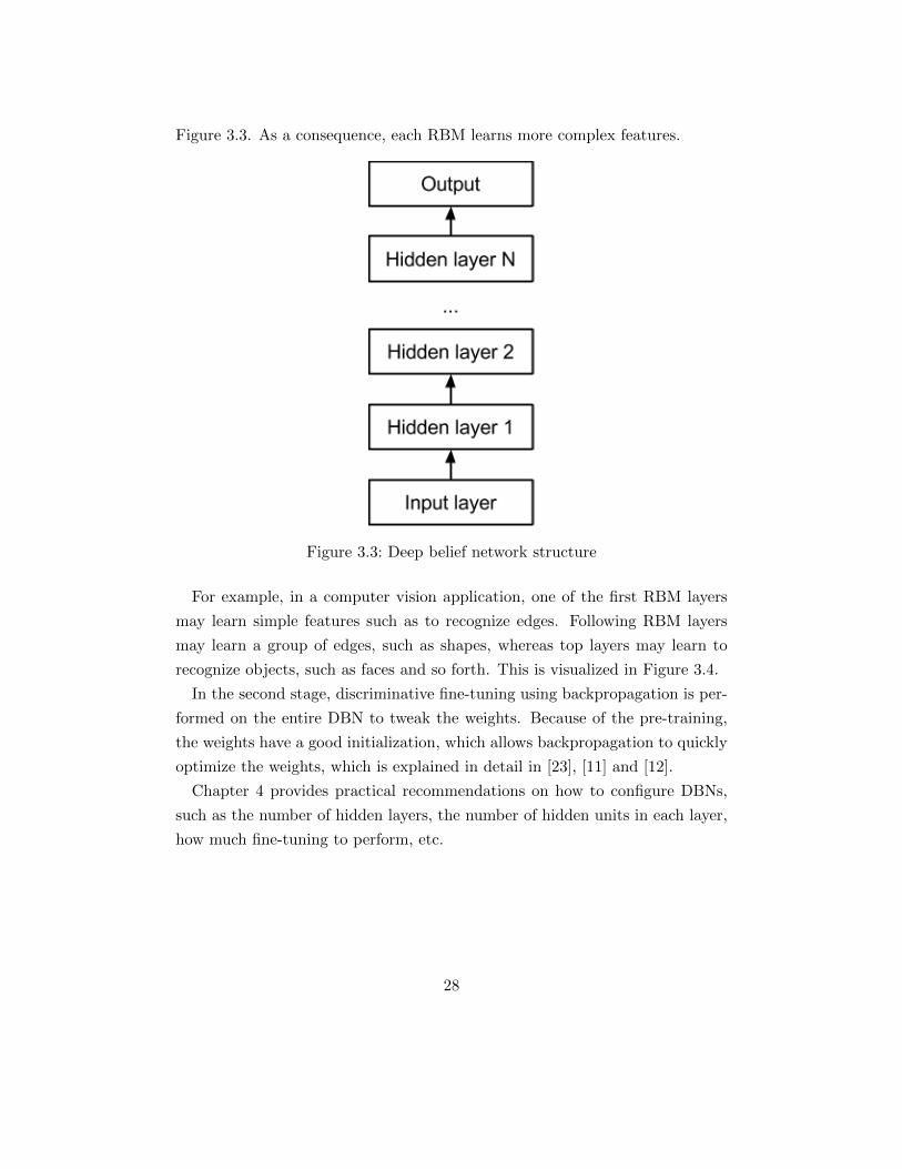
Figure 3.3. As a consequence, each RBM learns more complex features.

Figure 3.3: Deep belief network structure

For example, in a computer vision application, one of the first RBM layers

may learn simple features such as to recognize edges. Following RBM layers

may learn a group of edges, such as shapes, whereas top layers may learn to

recognize objects, such as faces and so forth. This is visualized in Figure 3.4.

In the second stage, discriminative fine-tuning using backpropagation is per-

formed on the entire DBN to tweak the weights. Because of the pre-training,

the weights have a good initialization, which allows backpropagation to quickly

optimize the weights, which is explained in detail in [23], [11] and [12].

Chapter 4 provides practical recommendations on how to configure DBNs,

such as the number of hidden layers, the number of hidden units in each layer,

how much fine-tuning to perform, etc.

28

Figure 3.4: Deep belief network layers learning complex feature hierarchies [41]

3.4.1 Stacked autoencoders

Building a DBN from autoencoders is also called a stacked autoencoder. The

learning process is related to constructing a DBN from RBMs, in particular the

layer-wise pre-training, as explained in [21]. First, an autoencoder is trained on

the input. The trained hidden layers serves then as the first hidden layer of the

stacked autoencoder. Second, the features learned by the hidden layer are used

as input and output to train another autoencoder. The learned hidden layer of

the second autoencoder is then used as the second hidden layer of the stacked

autoencoder. This process can be continued for multiple autoencoders, similarly

to training a DBN composed of RBMs. Similarly, each hidden layer learns

more complex features. Last, fine-tuning of the weights using backpropagation

is performed on the stacked autoencoder.

3.5 Further approaches

This section briefly covers alternative approaches that are used to train deep

neural networks.

29

3.5.1 Discriminative pre-training

Starting with a single hidden layer, a neural network is trained discriminatively.

Subsequently, a second hidden layer is inserted between the first hidden layer

and the output layer. Next, the whole network is trained discriminately again.

This process can be repeated for more hidden layers. Finally, discriminative

fine-tuning is performed in order to tweak the weights. This method is called

discriminative fine-tuning and described by Hinton in [20].

3.5.2 Hessian-free optimization and sparse initialization

Based on Newton’s method for finding approximations to the roots of a real-

valued function, a function l can be minimized by performing Newton’s method

on its first derivative. This method can be generalized to several dimensions:

θ := θ −H−1∇θl(θ) (3.17)

The gradient ∇θl(θ) is the vector of partial derivatives of l(θ) with respect

to the θi’s. The Hessian H is an n-by-n matrix of partial derivatives:

Hij =∂2l

∂θi∂θj

Because of calculating and inverting the Hessian, each iteration of Newton’s

method is more expensive than one iteration of gradient descent. Instead, this

method converges usually much faster than gradient descent. So-called quasi-

Newton methods approximate the Hessian instead of calculating it explicitly.

[24] presents a so-called Hessian-free approach, which allows to calculate

a helper matrix accurately using finite differences and does not require pre-

training. It is combined sparse initialization of weights, i.e. by setting most

incoming connection weights to each unit to zero.

3.5.3 Reducing internal covariance shift

As described in [39], during training, a change of the parameters of the previous

layers causes the distribution of each layer’s input to change. This so-called

30

internal covariance shift slows down training and may result in a neural network

that overfits. Internal covariance shift can be compensated by normalizing the

input of every layer. As a consequence, training can be significantly accelerated.

The resulting neural network is also less likely to overfit. This approach is

dramatically different to regularization covered in Chapter 2.4, as it addresses

the cause of overfitting, rather than trying to improve a model that overfits.

31

4 Practical recommendations

The concepts described in Chapter 3 allow to build powerful deep neural net-

works in theory. Yet, there are many open questions on how to tweak them in

order to achieve cutting-edge results in applications. This chapter provides an

overview about selected practical recommendations and improvements result-

ing from them, collected from a variety of publications. It also includes selected

examples of improved classification rates for concrete examples. Furthermore,

this chapter contains elaborations and critical comments by the author of this

report on the suggested practical recommendation where necessary.

4.1 Activation functions

Typical neural networks use linear or Sigmoidal activation functions in their

output layer for regression or classification, respectively. For deep neural net-

works, other activation functions have been proposed, which are covered in this

section. Softmax is a generalization of the Sigmoid activation function, based

on the following relation, covered in [16]:

p = σ(x) =1

1 + e−x=

ex(1)

ex(1 + e−x)=

ex

ex + e0(4.1)

This can be generalized to K output units:

pj =exj∑Ki=1 e

xi(4.2)

It is used in the output layer. As described by Norvig in [34], the output

of a unit becomes almost deterministic for a unit that is much stronger than

the others. Another benefit of softmax is that it is always differentiable for a

32

weight. As recommended in [50] and [6], softmax is ideally combined with the

cross-entropy cost function, which is covered in Chapter 2.3.

In order to model the behavior or neurons more realistically, the rectified

linear unit activation function has been proposed in [44]:

f(x) = max(0, x) (4.3)

This non-linearity allows to only activate a unit if its output is positive. There

is also a smooth approximation of this activation, which is differentiable:

f(x) = log(1 + ex) (4.4)

Another proposed activation function is a maxout network, which groups the

values of multiple units and select the strongest activation, covered in [46] and

[28].

Significant improvements of classification rates using rectified linear units and

maxout networks have been reported in [46] and [51] for speech recognition and

computer vision tasks. In particular, combinations of maxout, convolutional

neural networks and dropout, see Chapters 2.2 and 2.4.4, respectively, have

been reported. For example, [32] compares the performance of different neural

networks on the MNIST dataset. It starts with a standard neural network and

a SVM using the radial basis function kernel having error rates of 1.60% and

1.40%, respectively. It then presents various dropout neural networks using

rectified linear units with errors around 1.00% and a dropout neural network

using maxout units with error of 0.94%. Deep belief networks and so-called deep

Boltzmann machines using fine-tuned dropout achieved error rates of 0.92% and

0.79%, respectively.

4.2 Architectures

As discussed in Chapter 2.1, there are many different (and opposing) guidelines

on the architecture of neural networks. The same considerations apply to deep

neural networks. In general, the more units and the more layers, the more

33

complex hypotheses can be learned by a network. Considering each hidden

layer as a feature detector, the more layers, the more complex feature detectors

can be learned. As a consequence, a very deep network tends to overfit and

therefore requires strong regularization or more data.

Finding a good architecture for a specific task is a model selection problem

and is linked to specific training choices made, which are covered in Chapter 4.3.

Different observations and results on architecture evaluations have been repor-

ted in the literature, for example in [17] and [11] on MNIST.

For layer-wise pre-training of RBMs, Hinton provides a vague recipe for ap-

proximating the number of hidden units of a RBM in [16]. No further details

on the justification of this recipe are provided. In order to reduce overfitting,

the number of bits to describe a data vector must be approximated first, for

example using entropy. Second, this number should be multiplied with the

number of training cases. The number of units should then be an order of

magnitude smaller of that product. Hinton adds that for very sparse models,

more units may be picked, which makes intuitively sense, as sparsity itself is

a form of regularization, as discussed in Chapter 3.2.2. Furthermore, he notes

that large datasets are prone to high redundancy, for which he recommends less

units in order to compensate the risk of overfitting.

4.3 Training of RBMs and autoencoders

This section summarizes recommendations concerning the training of RBMs

and autoencoders. Hinton and Ng provide details on training RBMs and au-

toencoders in [16] and [6], respectively.

4.3.1 Variations of gradient descent in RBMs

Hinton proposes to use small initial weights in RBMs. Similar to the difficulty

of training regular feed-forward networks discussed in Chapter 2.3, larger initial

weights may speed up learning, but would result in a model prone to overfit-

ting. Concretely, he proposes initial weights drawn from a zero-mean Gaussian

distribution with a small standard deviation of 0.01. For the bias terms, he

34

proposes to set the hidden biases to 0 and the visible biases to log(pi/(1− pi))with pi being the fraction of training examples in which unit i is activated.

Mini-batch gradient descent

Stochastic gradient descent defined in Algorithm 2.2 is the choice for training

neural networks. Hinton recommends to use mini-batch gradient descent, which

is defined in Algorithm 4.1.

Algorithm 4.1 Mini-batch gradient descent: training size m, learning rate α

b← batch sizerepeat

for i = 1 to m, step = b doθj ← θj − α ∂

∂θjJ(θ, (x(i), y(i)), ..., (x(i+step), y(i+step))) (simultaneously

for all j)end for

until convergence

Comparing (batch) gradient descent defined in Algorithm 2.1 to stochastic

gradient descent, it can be concluded that mini-batch gradient descent is a

combination of both algorithms. This algorithm computes the parameters for

batches of b training examples. Mini-batch gradient allows like stochastic gradi-

ent descent to move quickly towards a minimum and the possibility to escape

from local minima. In addition it can be vectorized. Vectorization represents

k training examples in a matrix:

X =

——(x(1))T——

——(x(2))T——...

——(x(k))T——

(4.5)

Gradient descent can then be computed in a sequence of matrix operations.

Efficient algorithms such as the Strassen algorithm defined in [43] compute

matrix multiplications in O(nlog27) ≈ O(n2.807) instead of the naive multiplic-

ation which is O(n3). The idea behind the Strassen algorithm is to define a

35

matrix multiplication in terms of recursive block matrix operations. Exploiting

redundancy among the block matrices, it results in less multiplications. The

Strassen algorithm comes with runtime performance gains, both because of less

multiplications and is also able to be parallelized, making it an ideal candidate

for executing in a GPU.

The batch size of the mini-batches must be well balanced. If it is too large,

the algorithm’s behavior is close to gradient descent and if it is too small, no

advantage of vectorization can be taken. Hinton recommends to set the batch

size equal the number of classes and to put a training example of each class in

each every batch. If this is not possible, he recommends to randomly shuffle the

training set first and then to use a batch size of about 10. As efficient matrix

multiplications come with a large constant, Ng notes in [4] that many libraries

do not apply it to small matrices, as the naive multiplication is often faster in

such cases. Elaborating on this, it can be concluded that a larger batch size

than 10 is probably more useful for runtime performance gains, ideally with a

number of training examples close to the number of features and both being

slightly less or equal to a power of 2, as the Strassen algorithm expands matrix

dimensions to a power of 2.

Learning rate

For any gradient-based learning algorithm, setting the learning rate α is crucial.

A too small learning rate will make a learning algorithm converge too slowly. In

contrast, a too large learning rate will make the learning algorithm overshoot

and possibly lead to significant overfitting. Hinton recommends to generate

histograms of weight updates and weight values. The learning rate should then

be adjusted to scale the weight updates to about 0.1% of the weight values, but

provides no further justification for that choice.

Momentum

Furthermore, Hinton proposes to combine the weight updates with momentum,

which allows to speed up learning through long and slowly decreasing ”valleys”

in a cost function, but increasing the velocity of the weight updates. In the

36

simplest method, a learning rate could be simply multiplied by 1/(1 − µ) in

order to speed learning up. Alternatively, the weight update is then computed,

where α is the learning rate:

∆θi(t) = µ∆θi(t− 1)− α∂J(Θ)

∂θi(t) (4.6)

In order to compute the weight update, the previous weight update is taken

into account. The weight update is then accelerated by a factor of 1/(1 − µ)

if the gradient has not changed. Hinton notes that this update rule applying

temporal smoothing is more reliable than the basic method discussed initially.

He proposes to start with a low momentum value µ of 0.5 giving an update

factor of 1/(1− 0.5) = 2 for parameter updates, as random initial weights may

cause large gradients. A too large momentum value could cause the algorithm

to overshoot by oscillating, which is less likely giving a low momentum value.

More details on weight initialization and momentum are provided in [23].

Hinton adds that L1 and L2 regularization can be used as well for the training

of RBMs.

4.3.2 Autoencoders

For autoencoders, there have been less recommendations available in the liter-

ature. Most prominently, Ng’s tutorial in [6] provides advice on training au-

toencoders. In particular, that tutorial provides advice on data preprocessing,

which helps to improve the performance of deep learning algorithms as stated

in the tutorial. It covers mean-normalization, feature scaling and whitening, a

decorrelation procedure. As explained by Ng, whitening is particularly helpful

to process image data, which contains large redundancies, and preprocessing

led to significantly better results. Preprocessing then also helps to visualize the

features learned by the units, as visualized in Figure 4.1. Concretely, it shows

the input image that maximally activates each of the 100 hidden units.

Furthermore, [11] provides a study on the number of hidden layers of stacked

autoencoders for the MNIST dataset, with 4 layers being the best tradeoff of

over- and underfitting.

37

Figure 4.1: Features learned by 100 hidden units of the same layer [6]

4.3.3 Fine-tuning of DBNs

The effect of fine-tuning has been extensively evaluated in [17] on MNIST by

Hinton. He starts with a pre-trained DBN. Pre-trained DBNs usually already

have a good classification rate, as their feature detectors are learned from the

training data. Hinton highlights that only a small learning rate should be picked

in order to not change the network weights too much in the fine-tuning stage.

He then applies backpropagation fine-tuning with early stopping to reduce clas-

sification errors to about 1.10%.

As investigated in [22], fine-tuning may result in strong overfitting. Whether

doing it at all should therefore be subject to model selection, not just the

number of epochs and when to stop.

38

5 Application to computer vision

problems

This chapter applies some of the methods of the previous chapters to real

learning problems. Different methods are compared on two databases and their

results are presented.

5.1 Available databases

This section briefly covers the two databases that are of interest for the exper-

iments of this report.

5.1.1 MNIST

The Mixed National Institute of Standards and Technology (MNIST) database

[49] is a collection of handwritten digits with different levels of noise and dis-

tortions. It was initially created by LeCun for his research on convolutional

neural networks in the 1980s shown in Figure 5.1.

It is used in many papers on deep learning to which there have been numerous

references. For example, [32] and [18] report error rates of 1.05% and 1.2%,

respectively. It is important to bear in mind that these error rates were only

achieved applying many different tweaks and optimizations, which are partially

covered in Chapter 4.

In the following experiments, the MNIST dataset that comes with the MAT-

LAB Deep Learning Toolbox, introduced in Chapter 5.2.2, is used. It has 60000

training examples and 10000 test examples. Each example contains 28×28 pixel

gray-scale values, of which most are set to zero.

39

Figure 5.1: Hand-written digit recognition learned by a convolutional neuralnetwork [47]

5.1.2 Kaggle facial emotion data

Kaggle is a platform that hosts data mining competitions. Researchers and

data scientists compete with their models trained on a given training set in

order to achieve the best prediction on a test set. In 2013, a challenge named

”Emotion and identity detection from face images” [26] was hosted.

This challenge was won by a convolutional neural network presented in [45],

which achieved an error rate of 52.977%. In total, there were 72 submissions,

with 84.733% being the highest error rate and a median error rate of 63.255%.

The original training set contains 4178 training and 1312 test examples for

seven possible emotions. Each example contains 48 × 48 pixel gray values, of

which most are set to non-zero. Since the test labels are not available, the

original training set is split up into 3300 training and 800 test examples. Some

examples are visualized in Figure 5.2.

40

Figure 5.2: Sample data of the Kaggle competition [26]

5.2 Available libraries

This section briefly covers the two deep learning libraries that are of interest

for the experiments of this report.

5.2.1 Hinton library

Based on his paper [18], Hinton provides a MATLAB implementation of a

stacked autoencoder in [19]. This code is highly optimized and lacks gener-

alization to other problems. Since this report covers different databases and

different deep training methods, it is not further considered.

5.2.2 Deep Learning Toolbox

Palm provides a generic and flexible toolbox for deep learning in [36] based on

[37]. It includes implementations of deep belief networks composed of RBMs,

stacked (denoising) autoencoders, convolutional neural networks, convolutional

autoencoders and regular neural networks. Furthermore, it comes with ready

to use code examples for MNIST. These examples make the library easy to use

and demonstrate various possible configurations.

41

5.3 Experiments

For the following experiments on the two databases presented in Chapter 5.1,

Palm’s Deep Learning Toolbox introduced in Chapter 5.2.2 is used. This section

only covers very initial experiments to get a taste of the key training methods

covered in this report.

5.3.1 Classification of MNIST

In this section, deep belief networks composed of RBMs (DBN) are compared

to stacked denoising autoencoders (SAE) for the MNIST dataset, covered in

Chapters 3.

The MNIST input is normalized from integer values in [0, 255] to real val-

ues in [0, 1] and used throughout the following experiments. For both training

methods, a number of parameters are optimized independently. Table 5.1 con-

tains the different values of parameters that are tested on both training methods

throughout pre-training and fine-tuning.

Parameter Default value Tested values

Learning rate 1.0 0.25, 0.5, 0.75, 1.0, 1.25, 1.5,1.75, 2.0

Momentum 0 0.01, 0.02, 0.05, 0.1, 0.15, 0.2,0.25, 0.5

L2 regularization 0 1e-7, 5e-7, 1e-6, 5e-6, 1e-5, 5e-5,1e-4, 5e-4

Output unit type Sigmoid Sigmod, softmaxBatch size 100 25, 50, 100, 150, 200, 400

Hidden Layers [100, 100] [50], [100], [200], [400], [50, 50],[100, 100], [200, 200], [400, 400],

[50, 50, 50], [100, 100, 100],[200, 200, 200]

Dropout 0 0, 0.125, 0.25, 0.5

Table 5.1: Model selection values for MNIST

The parameters are optimized independently for computational performance

reasons. During the optimization, the other parameters are set to the default

42

values in Table 5.1. Figure 5.3 visualizes the test error for different L2 regular-

ization values, with an optimal value for 5e-5 of 0.0298.

Figure 5.3: Test error for different L2 regularization values for training of DBN

The same procedure is followed for the other parameters with 10 epochs for

both pre-training and fine-tuning. Table 5.2 includes the optimal values and

respective test errors for both DBN and SAE. Overall, the test errors are below

4% for the selected parameter values. Both training methods achieve the best

error rate improvement for a change of the number of hidden units from one

layer of 100 units to two layers of 400 units each.

Finally, the optimal values are put together for both training methods in

order to train two optimized classifiers. In addition, a regular non-denoising

stacked autoencoder is trained on these parameter values. Table 5.3 contains

the respective results.

The stacked denoising autoencoder achieves with a test error of 1.94% clearly

43

Parameter DBN Test error SAE Test error

Learning rate 0.5 0.0323 0.75 0.0383Momentum 0.02 0.0331 0.5 0.039

L2 regularization 5e-5 0.0298 5e-5 0.0345Output unit type softmax 0.0278 softmax 0.0255

Batch size 50 0.0314 25 0.0347Hidden Layers [400, 400] 0.0267 [400, 400] 0.017

Dropout 0 0.0335 0 0.039

Table 5.2: Model selection for DBN and SAE on MNIST, lowest error rates inbold

Neural network Test error

DBN composed of RBMs 0.0244Stacked denoising autoencoder 0.0194

Stacked autoencoder 0.0254

Table 5.3: Error rates for optimized DBN and SAE on MNIST, lowest errorrate in bold

the best result of the three classifiers. The DBN composed of RBMs performs

with an error rate of 2.44% in comparison to the stacked autoencoder with an

error rate of 2.54%.

Compared to the error rates reported in [32] and [18] of 1.05% and 1.2%,

the MATLAB Deep Learning Toolbox gets quite close to these best values

reported with simple parameter optimization and without any hacks in the

implementation limited to the concrete MNIST problem.

For an exhaustive optimization, the error rates are likely to go down further.

The single optimization of the architecture in Table 5.2 achieved an error of

1.7% for the stacked denoising autoencoder in comparison to the aggregation of

optimized values in Table 5.3. Furthermore, significantly increasing the number

of epochs is likely to further reduce the error rates.

5.3.2 Classification of Kaggle facial emotion data

In this section, deep belief networks composed of RBMs (DBN) are compared

to stacked denoising autoencoders (SAE) for the Kaggle facial emotion dataset,

44

covered in Chapters 3.

Each data point has 48 × 48 = 2304 pixels. As there are only 3300 training

examples, initial experiments returned impractical error rates of 90%. One of

the reasons is the low ratio of the number of training examples and the number

of features. Therefore, the image size is reduced to 24×24 = 576 pixels using a

bilinear interpolation. Using the nearest 2-by-2 neighborhood, the result pixel

value is a weighted average of pixels in the neighborhood. Subsequently, the

input is normalized from integer values in [0, 255] to real values in [0, 1] and

used throughout the following experiments.

Similar to the model selection for MNIST in Chapter 5.3.1, for both train-

ing methods, a number of parameters are optimized independently. Table 5.4

contains the different values of parameters that are tested on both training

methods throughout pre-training and fine-tuning.

Parameter Default value Tested values

Learning rate 1.0 0.05, 0.1, 0.15, 0.25, 0.5, 0.75, 1.0,1.25, 1.5

Momentum 0 0.01, 0.02, 0.05, 0.1, 0.15, 0.2,0.25, 0.5

L2 regularization 0 1e-7, 5e-7, 1e-6, 5e-6, 1e-5, 5e-5,1e-4, 5e-4

Output unit type Sigmoid Sigmod, softmaxBatch size 100 25, 50, 100, 150, 275

Hidden Layers [100, 100] [50], [100], [200], [400], [50, 50],[100, 100], [200, 200], [400, 400],

[50, 50, 50], [100, 100, 100],[200, 200, 200]

Dropout 0 0, 0.125, 0.25, 0.5

Table 5.4: Model selection values for Kaggle data

The parameters are also optimized independently for computational perform-

ance reasons. During the optimization, the other parameters are set to the

default values in Table 5.4. Figure 5.4 visualizes the test error for different

learning rates, with an optimal value for 0.1 of 0.5413.

The same procedure is followed for the other parameters with 10 epochs

45

Figure 5.4: Test error for different learning rates values for training of DBN

for both pre-training and fine-tuning. Table 5.5 includes the optimal values

and respective test errors for both DBN and SAE. Overall, the test errors are

high for the selected parameter values. As discussed in Chapter 5.1.2, the best

contribution has an error rate of 52.977%. Also, in many instances of the model

selection, the test error plateaus on 72.25%. This is most likely caused by the

noise and redundancy in the data set and the overall low amount of training

examples. Possible solutions are discussed at the end of this experiment.

Finally, the optimal values are put together for both training methods in

order to train two optimized classifiers. In addition, a regular non-denoising

stacked autoencoder is trained on these parameter values. Table 5.6 contains

the respective results.

Both, the DBN composed of RBMs and the stacked denoising autoencoder

plateau at an error rate of 72.25%. Interestingly, using the same parameter

46

Parameter DBN Test error SAE Test error

Learning rate 0.25 0.5587 0.1 0.5413Momentum 0.01 0.7225 0.5 0.7225

L2 regularization 5e-5 0.7225 1e-4 0.7225Output unit type softmax 0.7225 softmax 0.7225

Batch size 50 0.6987 50 0.5913Hidden Layers [50, 50] 0.7225 [200] 0.5850

Dropout 0.125 0.7225 0.5 0.7225

Table 5.5: Model selection for DBN and SAE on Kaggle data, lowest error ratesin bold

Neural network Test error

DBN composed of RBMs 0.7225Stacked denoising autoencoder 0.7225

Stacked autoencoder 0.3975

Table 5.6: Error rates for optimized DBN and SAE on Kaggle data, lowest errorrate in bold

values of the stacked denoising autoencoder for a regular stacked autoencoder,

the test error goes down to 39.75%. This is clearly a major advancement to the

best Kaggle contribution with an error of 52.977%. However, it must be noted

that the test set is not identical, since the test labels are not available, which

required the original training set to be split into training and test data. Bearing

this in mind, the learning problem in this experiment may even be harder since

less training examples are available.

More advanced pre-processing methods are the Principal Component Ana-

lysis (PCA) or whitening discussed and recommended for gray-scale images in

[6]. Using PCA, only a relevant fraction of the features can be used for the

learning in order to reduce the plateau of 72.25% and to speed up learning.

Gray-scale images are highly-redundant and using whitening, the features can

be decorrelated in order to further improve error rates. Furthermore, limit-

ations in the implementation of the toolbox may also contribute to the high

plateau of error rates. For example, linear units in the visible layer of the

RBMs could also handle the input better and may improve error rates. Also,

47

as for the MINIST dataset, significantly increasing the number of epochs is

likely to further reduce the error rates.

48

6 Conclusions and prospects

Neural networks have a long history in machine learning that came with re-

peating rise and enthusiasm followed by loss popularity. Neural networks are

known to have a high expressional power in order to model complex non-linear

hypotheses. In practice, training deep neural networks using the backpropaga-

tion algorithm is difficult. Their large number of weight parameters result

in highly non-convex cost functions that are difficult to minimize. As a con-

sequence, training often converges to local minima, resulting in overfitting and

lower generalization errors.

Over the last ten years, a number of new training methods have been de-

veloped in order to pre-train neural networks resulting in a good initialization

of their weights. These weights can then be fine-tuned using backpropagation.

The most popular pre-training methods in order to construct deep neural net-

works are Restricted Boltzmann Machines (RBMs) and Autoencoders. Aside

from these concepts, there are other methods and approaches such as discrim-

inative pre-training and dropout regularization. Furthermore, there are many

practical recommendations to tweak these methods.

As shown in the experiments, deep neural network training methods are

powerful and achieve very high classification rates in different computer vision

problems. Nonetheless, deep learning is not a concept that can be used out of

the box, as proper pre-processing of the data and extensive model selection are

necessary.

It would be interesting to apply more powerful pre-processing methods to the

data, such as PCA or whitening. Furthermore, convolutional neural networks

have been reported in the literature to perform very well on computer vision

problems, which would be interesting to study, too. In order to speed up learn-

ing, use of GPUs has been successfully used in the literature. These methods

49

also look promising to be applied to the problems covered in this report.

50

Bibliography

[1] Adam Coates, Brody Huval, Tao Wang, David J. Wu, Bryan Catanzaro

and Andrew Ng: Deep Learning with COTS HPC Systems. Stanford.

2013.

[2] Andrew Ng: Deep Learning, Self-Taught Learning and Unsupervised

Feature Learning. http://www.youtube.com/watch?v=n1ViNeWhC24.

Retrieved: February 15, 2015.

[3] Andrew Ng: Feature selection, L1 vs. L2 regularization, and rotational

invariance. Stanford. 2004.

[4] Andrew Ng: Machine Learning. Coursera. 2014.

[5] Andrew Ng: Machine Learning. Stanford. 2014.

[6] Andrew Ng et al.: Deep Learning Tutorial.

http://deeplearning.stanford.edu/tutorial/. Retrieved: February

27, 2015.

[7] Quora: How is a Restricted Boltzmann machine different from an

Autoencoder? Aren’t both of them learning high level features in an

unsupervised manner? Similarly, how is a Deep Belief Network different

from a network of stacked Autoencoders?. http://goo.gl/5V7r61.

Retrieved: March 1, 2015.

[8] Christopher M. Bishop: Pattern Recognition and Machine Learning.

Springer. 2007.

[9] David Lowe: Object recognition from local scale-invariant features.

Proceedings of the International Conference on Computer Vision 2,

1150-1157. 1999.

51

[10] Dean A. Pomerleau: ALVINN, an autonomous land vehicle in a neural

network. Carnegie Mellon. 1989.

[11] Dumitru Erhan, Pierre-Antoine Manzagol and Yoshua Bengio and Samy

Bengio and Pascal Vincent: The Difficulty of Training Deep

Architectures and the Effect of Unsupervised Pre-Training. Twelfth

International Conference on Artificial Intelligence and Statistics

(AISTATS). 2009.

[12] Dumitru Erhan, Yoshua Bengio, Aaron Courville, Pierre-Antoine

Manzagol, Pascal Vincent and Samy Bengio: Why Does Unsupervised

Pre-training Help Deep Learning?. Journal of Machine Learning

Research, 11 (Feb), 625?660. 2010.

[13] Edwin Chen: Introduction to Restricted Boltzmann Machines.

http://blog.echen.me/2011/07/18/

introduction-to-restricted-boltzmann-machines/. 2011.

Retrieved: February 15, 2015.

[14] Eugene Wong: Stochastic Neural Networks. Algorithmica, 6, 466-478.

1991.

[15] Frank Rosenblatt: Principles of neurodynamics; perceptrons and the

theory of brain mechanisms. Washington: Spartan Books. 1962.

[16] Geoffrey Hinton: A Practical Guide to Training Restricted Boltzmann

Machines. UTML TR 2010-003, University of Toronto. 2010.

[17] Geoffrey Hinton: To Recognize Shapes, First Learn to Generate Images.

UTML TR 2006-004, University of Toronto. 2006.

[18] Geoffrey Hinton and R. Salakhutdinov: Reducing the dimensionality of

data with neural networks. Science, 313 (5786), 504-507. 2006.

[19] Geoffrey Hinton and R. Salakhutdinov: Training a deep autoencoder or

a classifier on MNIST digits. http:

//www.cs.toronto.edu/~hinton/MatlabForSciencePaper.html.

Retrieved: April 22, 2015.

52

[20] Geoffrey Hinton et al.: Deep Neural Networks for Acoustic Modeling in

Speech Recognition. IEEE Signal Processing Magazine, 29 (6), 82-97.

2012.

[21] Hugo Larochelle, Isabelle Lajoie and Yoshua Bengio: Stacked Denoising

Autoencoders: Learning Useful Representations in a Deep Network with

a Local Denoising Criterion. The Journal of Machine Learning Research,

11, 3371-3408. 2010.

[22] Hugo Larochelle, Yoshua Bengio, Jerome Louradour and Pascal

Lamblin: Exploring Strategies for Training Deep Neural Networks. The

Journal of Machine Learning Research, 10, 1-40. 2009.

[23] I. Sutskever, J. Martens, G. Dahl, and G. Hinton: On the importance of

momentum and initialization in deep learning. 30th International

Conference on Machine Learning. 2013.

[24] James Martens: Deep learning via Hessian-free optimization.

Proceedings of the 27th International Conference on Machine Learning

(ICML). 2010.

[25] Jeff Heaton: Introduction to Neural Networks for Java. 2nd Edition,

Heaton Research. ISBN 1604390085. 2008.

[26] Kaggle: Emotion and identity detection from face images.

http://inclass.kaggle.com/c/facial-keypoints-detector.

Retrieved: April 15, 2015.

[27] Li Deng, Mike Seltzer, Dong Yu, Alex Acero, Abdel-rahman Mohamed

and Geoff Hinton: Binary Coding of Speech Spectrograms Using a Deep

Auto-encoder. Interspeech, International Speech Communication

Association. 2010.

[28] Li Deng and Dong Yu: Deep Learning Methods and Applications.

Foundations and Trends in Signal Processing, 7 (3-4), 197-387. 2014.

53

[29] M. Liu, S. Li, S. Shan and X. Chen: AU-aware Deep Networks for facial

expression recognition. 10th IEEE International Conference and

Workshops on Automatic Face and Gesture Recognition (FG). 2013.

[30] Marvin Minsky and Seymour Papert: Perceptrons: An Introduction to

Computational Geometry. M.I.T. Press. 1969.

[31] Melanie Mitchell: An Introduction to Genetic Algorithms. M.I.T. Press.

1996.

[32] Nitish Srivastava, Geoffrey Hinton, Alex Krizhevsky, Ilya Sutskever,

Ruslan Salakhutdinov: Dropout: A Simple Way to Prevent Neural

Networks from Overfitting. The Journal of Machine Learning Research,

15, 1929-1958, 2014.

[33] P. Liu, S. Han, Z. Meng and Y. Tong: Facial Expression Recognition via

a Boosted Deep Belief Network. IEEE Conference on Computer Vision

and Pattern Recognition (CVPR). 2014.

[34] Peter Norvig and Stuart J. Russell: Artificial Intelligence: A Modern

Approach. Prentice Hall. Third Edition. 2009.

[35] Quoc Le, Marc’Aurelio Ranzato, Rajat Monga, Matthieu Devin, Kai

Chen, Greg Corrado, Jeff Dean and Andrew Ng: Building high-level

features using large scale unsupervised learning. International

Conference in Machine Learning. 2012.

[36] Rasmus Berg Palm: DeepLearnToolbox.

http://github.com/rasmusbergpalm/DeepLearnToolbox. Retrieved:

April 22, 2015.

[37] Rasmus Berg Palm: Prediction as a candidate for learning deep

hierarchical models of data. 2012.

[38] Richard O. Duda: Pattern Classification. Wiley-Interscience. Second

Edition. 2000.

54

[39] Sergey Ioffe, Christian Szegedy: Batch Normalization: Accelerating

Deep Network Training by Reducing Internal Covariate Shift. Google.

2015.

[40] Stackoverflow: Estimating the number of neurons and number of layers

of an artificial neural network. http://goo.gl/lIaxVY. Retrieved:

February 10, 2015.

[41] The Analytics Store: Deep Learning.

http://theanalyticsstore.com/deep-learning/. Retrieved: March

1, 2015.

[42] Tom Mitchell: Machine Learning. McGraw Hill. 1997.

[43] Volker Strassen: Gaussian Elimination is not Optimal. Numer. Math.

13, 354-356. 1969.

[44] Vinod Nair and Geoffrey E. Hinton: Rectified Linear Units Improve

Restricted Boltzmann. 2010.

[45] Y. Tang: Challenges in Representation Learning: Facial Expression

Recognition Challenge Implementation. University of Toronto. 2013.

[46] Yajie Miao, F. Metze and S. Rawat: Deep maxout networks for

low-resource speech recognition. IEEE Workshop on Automatic Speech

Recognition and Understanding (ASRU), 398-403. 2013.

[47] Yann LeCun et al.: LeNet-5, convolutional neural networks.

http://yann.lecun.com/exdb/lenet/. Retrieved: April 22, 2015.

[48] Yann LeCun: Research profile.

http://yann.lecun.com/ex/research/index.html. Retrieved:

February 28, 2015.

[49] Yann LeCun et al.: The MNIST database.

http://yann.lecun.com/exdb/mnist/. 1998.

[50] Yoshua Bengio: Learning Deep Architectures for AI. Foundations and

Trends in Machine Learning, 2 (1), 1-127. 2009.

55

[51] Xiaohui Zhang, J. Trmal, J. Povey and S. Khudanpur: Improving deep

neural network acoustic models using generalized maxout networks.

IEEE International Conference on Acoustics, Speech and Signal

Processing (ICASSP), 215-219. 2014.

56