COMPARISON OF THE DISCRETE SINGULAR CONVOLUTION

COMPARISON OF THE DISCRETE SINGULAR CONVOLUTIONAND THREE OTHER NUMERICAL SCHEMES FOR

SOLVING FISHER’S EQUATION∗

SHAN ZHAO† AND G. W. WEI‡

SIAM J. SCI. COMPUT. c© 2003 Society for Industrial and Applied MathematicsVol. 25, No. 1, pp. 127–147

Abstract. In this paper, a discrete singular convolution (DSC) algorithm is introduced to solveFisher’s equation, to which obtaining an accurate and reliable traveling wave solution is a challengingnumerical problem. Two novel numerical treatments, a moving frame scheme and a new asymptoticscheme, are designed to overcome the subtle difficulties involved in the numerical solution of Fisher’sequation. The moving frame scheme is proposed to provide accurate and efficient spatial resolution ofthe problem. The new asymptotic scheme is introduced to facilitate the correct prediction of the wavespeed after long-time integrations. The resulting DSC algorithm is able to correctly predict long-timetraveling wave behavior. The performance of the present algorithm is demonstrated through extensivenumerical experiments as well as through a comparison with three other standard approaches, i.e.,methods of the Fourier pseudospectral, the accurate spatial derivatives, and the Crank–Nicolsonschemes. The spatial and temporal accuracies of all four methods are analyzed and numericallyverified.

Key words. Fisher’s equation, discrete singular convolution, Fourier pseudospectral method

AMS subject classifications. 35K15, 65M06, 65M70, 65M99

DOI. 10.1137/S1064827501390972

1. Introduction. Fisher [3] introduced a one-dimensional nonlinear parabolicpartial differential equation (PDE) to describe the kinetic advancing rate of an ad-vantageous gene,

∂u

∂t= µ

∂2u

∂x2+ ρu(1 − u), x ∈ (−∞,∞), t > 0,(1.1)

where the positive quantities µ and ρ are the diffusion coefficient and the reactionfactor, respectively. Fisher’s equation represents the evolution of the population dueto the two competing physical processes, diffusion and nonlinear local multiplication.Equation (1.1) also describes a prototype model for a spreading flame [9] and a modelequation for the finite domain evolution of neutron population in a nuclear reactor[1].

It is convenient to nondimensionalize (1.1) by means of the transformation t := ρt,x := (ρ/µ)1/2x so that Fisher’s equation returns a simpler form,

∂u

∂t=

∂2u

∂x2+ u(1 − u).(1.2)

With the assumption that the saturation level is unity, the different initial and bound-ary conditions (BCs) for Fisher’s equation read

∗Received by the editors October 15, 2001; accepted for publication (in revised form) March 17,2003; published electronically September 9, 2003. This work was supported in part by the NationalUniversity of Singapore and Michigan State University.

http://www.siam.org/journals/sisc/25-1/39097.html†Department of Computational Science, National University of Singapore, Singapore 117543

([email protected]).‡Department of Mathematics, Michigan State University, East Lansing, MI 48824

([email protected]).

127

128 SHAN ZHAO AND G. W. WEI

u(x, 0) = u0(x) ∈ [0, 1], x ∈ (−∞,∞),(1.3)

limx→−∞u(x, t) = 1, lim

x→∞u(x, t) = 0,(1.4)

limx→±∞u(x, t) = 0,(1.5)

with the x derivative tending to zero as x → ±∞. In the literature, conditions (1.3)and (1.4) together are commonly referred to as nonlocal conditions, while conditions(1.3) and (1.5) together are usually referred to as local conditions.

The properties of Fisher’s equation have been studied theoretically by many au-thors, including Fisher [3], Kolmogorov, Petrovshy, and Piscounoff [9], Canosa [1],Larson [10], Hagan [7], etc. For the nonlocal conditions (1.3) and (1.4), it is provedin [9] that for every value of c ≥ 2, there exists a traveling wave solution to (1.2) witha wave speed c. No such solution exists if c < 2. The traveling wave solution can beexpressed in the form u(x, t) = V (x− ct) for a certain function V of the single scalarindependent variable z = x − ct. Such a solution is bounded as u0(x) in (1.3), i.e.,V (z) ∈ [0, 1] for any z ∈ R. For a given initial datum, the wave speed of the steadystate solution of Fisher’s equation is unique. Larson [10] and Hagan [7] discovered aninteresting phenomenon in which the steady state wave speed depends crucially onthe behavior of the initial datum at infinity. In particular, if u0(x) ∼ e−βx as x → ∞,then, as t → ∞, the solution evolves to a traveling wave of speed c(β) given by

c(β) =

{β + 1

β , β ≤ 1,

2, β ≥ 1.(1.6)

The traveling wave solution of Fisher’s equation has also been studied numericallyby many researchers because the accurate and reliable numerical representation of thetraveling wave solution to Fisher’s equation is an interesting and challenging numericalproblem. Numerous computational approaches have been applied to Fisher’s equationin the literature, including the method of accurate space derivatives (ASD) [6], finitedifferences [8, 13, 14], finite elements [20, 2, 18], as well as many others [15, 22, 12,11, 16, 17].

In any numerical study of Fisher’s equation, the infinite physical domain has to betruncated into a finite computational domain [xL, xR], with approximate BCs imposedat x = xL and x = xR. One of the most difficult numerical problems for the solutionof Fisher’s equation is the sensitivity of a correct numerical solution to the appropriateBCs, especially the one imposed at the right-hand boundary [6, 8, 16]. Theoreticalstudy reveals that it is the initial data at infinity that determine the traveling speed ofthe steady state wave solution. In numerical studies, the wave speed of the simulatedtraveling wave is determined by the BC applied on x = xR at each step of the timeintegration. Therefore, incorrect results would be obtained unless certain proper BCsare applied.

The commonly used BCs for Fisher’s equation in the literature [6, 15, 2, 17] includeu(xL, t) = 1 and u(xR, t) = 0 for nonlocal conditions and u(xL, t) = 0 and u(xR, t) = 0for local conditions. By using such BCs, Gazdag and Canosa [6] demonstrated thatthe superspeed wave (SSW) (the wave with speed c > 2) with theoretical speedc = 4 or c = 6 quickly evolves into the minimum speed wave. They also foundthat the time of evolving from SSW to the minimum speed wave depends cruciallyon the boundary cutoff point xR. Carey and Shen [2] reported similar results byusing a different numerical scheme under the same BCs. In some recent work onthe numerical solution of Fisher’s equation, Li, Petzold, and Ren [11] and Qiu and

SOLVING FISHER’S EQUATION 129

Sloan [16] avoided this difficulty by directly using the exact solution values in theDirichlet BC. However, this treatment is not applicable for general numerical studies.An interesting exception reported in the literature is the BC given by Hagstrom andKeller [8]. In terms of an asymptotic expansion form, their BC explicitly takes intoaccount the initial data in the discarded region x > xR. By using it, the travelingwave solutions with superspeed can be accurately represented on a finite domain.However, their BC is relatively complex and an explicit representation of the initialdata at infinity is required, which is actually unavailable in general.

Another difficulty of the numerical solution of Fisher’s equation is the instabilityof the traveling wave with respect to a small perturbation at the front of the wave[6, 7, 16]. It has been shown that the traveling wave is stable to a small disturbanceof compact support, while it is unstable under a small disturbance of infinite support[6, 7]. Qiu and Sloan further commented that perturbations at the wave front arevery significant compared with those at the rear of the wave. In numerical studies, asnoted by Carey and Shen [2], a slight negative value in the wave front will develop intoa noticeably negative undershoot. Therefore, the stability and reliability of numericalschemes are of crucial importance to the sound simulation of the long-term behaviorof the traveling wave solution.

Recently, Li, Petzold, and Ren [11] considered the numerical solution of a scaledFisher’s equation with very strong reaction. Under such strong reaction, the solutionevolves into a shock-like wave, which is difficult to resolve by using a uniform coarsegrid with a traditional lower-order scheme. The authors of [11] attacked the problemby using a popular moving mesh method able to dynamically generate a suitablenonuniform mesh. However, their results are not satisfactory. More recently, Qiu andSloan [16] re-examined the problem. They showed that by modifying the monitorfunction, the moving mesh method can perform well for the strong reaction case.

Most recently, the discrete singular convolution (DSC) algorithm [24] was pro-posed as a potential numerical approach for solving many computational problems,including Hilbert transform, analytic signal processing, and computational tomogra-phy. The mathematical foundations of the algorithm are the theory of distributionsand the theory of wavelets [28]. The use of the DSC algorithm was demonstrated bysolving problems of quantum eigenvalues [25], linear and nonlinear dynamics [26], in-compressible flows [29], and structural analysis [31, 32]. The DSC algorithm was alsosuccessfully utilized to facilitate a new synchronization scheme for shock capturing[30]. In [27], the unified feature of the DSC formalism was discussed and there it wasdemonstrated that computational methods of Galerkin, collocation, global, local, andfinite difference types can be derived from a single starting point in the framework ofthe DSC algorithm.

The objective of the present work is fourfold. First, we explore the use of the DSCalgorithm as a unified approach for solving Fisher’s equation. Our second objectiveis to make a comparison of the Fourier pseudospectral (FPS) method [19], the ASDapproach [6], the DSC scheme, and the Crank–Nicolson (CN) scheme for solvingFisher’s equation. Third, we introduce a moving frame method to resolve the shock-like wave. Finally, we propose a new asymptotic scheme to ensure a correct travelingspeed.

This paper is organized as follows. Section 2 is devoted to a brief descriptionof the DSC, CN, FPS, and ASD schemes. Section 3 gives some analyses of fournumerical schemes with respect to spatial resolution and time integration. Section 4presents the application of four numerical schemes to the solution of Fisher’s equation.


Only the nontrivial SSW is studied in the present work, since it is numerically verydifficult compared with the minimum speed wave. Extensive numerical experimentsare carried out to verify the theoretical analyses and to compare the accuracy, stability,flexibility, and efficiency of the four numerical schemes. Both the analytical solutionand the steady state wave speed are invoked for a quantitative validation of the presentapproaches. Conclusions are presented in section 5.

2. Numerical methods.

2.1. Discrete singular convolution. Singular convolutions are a special classof mathematical transformations which appear in many science and engineering prob-lems such as Hilbert transform, Abel transform, and Radon transform. It is mostconvenient to discuss the singular convolution in the context of the theory of distri-butions. Let T be a distribution and η(t) be an element of the space of test functions.A singular convolution is defined as

F (t) = (T ∗ η)(t) =

∫ ∞

−∞T (t− x)η(x)dx.(2.1)

Here T (t−x) is a singular kernel. Depending on the form of the kernel T , the singularconvolution is the central issue for a wide range of science and engineering problems.

An important example that is relevant to the present study involves the sin-gular kernels of delta type T (x) = δ(n)(x), (n = 0, 1, 2, . . .). Here, kernel T (x) =δ(x) is of particular importance for the interpolation. Higher-order kernels, T (x) =δ(n)(x), (n = 1, 2, . . .) are essential for numerically solving PDEs and for image pro-cessing, noise estimation, etc. However, since these kernels are singular, they cannotbe directly digitized in computers. Hence, the singular convolution, (2.1), is of lit-tle numerical merit. To avoid the difficulty of using singular expressions directlyin computers, we construct sequences of approximations (Tα) to the distribution T ,limα→α0 Tα(x) −→ T (x), where α0 is a generalized limit. Note that one retains thedelta distribution at the limit. Computationally, the Fourier transform of the deltadistribution is unity. Hence, it is a universal reproducing kernel for numerical com-putations and an all pass filter for image and signal processing. Therefore, the deltadistribution can be used as a starting point for the construction of either band-limitedreproducing kernels or approximate reproducing kernels. By the Heisenberg uncer-tainty principle, exact reproducing kernels have bad localization in the time (spatial)domain, whereas approximate reproducing kernels can be localized in both time andfrequency representations. Furthermore, with a sufficiently smooth approximation, itis useful to consider a DSC

Fα(t) =∑k

Tα(t− xk)f(xk),(2.2)

where Fα(t) is an approximation to F (t) and {xk} is an appropriate set of discretepoints on which the DSC, (2.2), is well defined. Note that the original test functionη(x) has been replaced by f(x). The mathematical property or requirement for f(x)is determined by the approximate kernel Tα.

The delta distribution or the so-called Dirac delta function (δ) is a generalizedfunction which is integrable inside a particular interval but in itself need not havea value. It is given as a continuous linear functional on the space of test functionsD(−∞,∞), 〈δ, φ〉 = δ(φ) =

∫∞−∞ δφ = φ(0). A delta sequence kernel, {δα(x)}, is a

sequence of kernel functions on (−∞,∞) which are integrable over every compact


domain, and their inner product with every test function φ converges to the deltadistribution

limα→α0

∫ ∞

−∞δαφ = 〈δ, φ〉,(2.3)

where the (real or complex ) parameter α approaches α0, which can be either ∞ or alimit value, depending on the situation (such a convention for α0 is used throughoutthis paper). If α0 represents a limit value, the corresponding delta sequence kernel isa fundamental family.

There are many delta sequence kernels arising in the theory of PDEs, Fouriertransforms, and signal analysis, with completely different mathematical properties.The delta sequence kernels of Dirichlet type have very distinct mathematical proper-ties and are used in the present work. Let {δα} be a sequence of functions on (−∞,∞)which are integrable over every bounded interval. We call {δα} a delta sequence kernelof Dirichlet type if

1.∫ a

−aδα → 1 as α → α0 for some finite constant a.

2. For every constant γ > 0, (∫ −γ

−∞ +∫∞γ

)δα → 0 as α → α0.

3. There are positive constants C1 and C2 such that |δα(x)| ≤ C1/|x| + C2 forall x and α.

Shannon’s delta sequence kernel (or Dirichlet’s continuous delta sequence kernel) isone of the most important examples of the delta sequence kernel of Dirichlet typeand is given by the following (inverse) Fourier transform of the characteristic func-

tion, χ[−α/(2π),α/(2π)]: δα(x) =∫∞−∞ χ[−α/(2π),α/(2π)]e

−i2πξxdξ = sin(αx)πx . Numerically,

Shannon’s delta sequence kernel is one of the most important cases because of itsproperty of being an element of the Paley–Wiener reproducing kernel Hilbert spaceB2

1/2,

f(x) =

∫ ∞

−∞f(y)

sinπ(x− y)

π(x− y)dy ∀f ∈ B2

1/2,(2.4)

where ∀f ∈ B21/2 indicates that, in its Fourier representation, the L2 function f

vanishes outside the interval [− 12 ,

12 ]. The Paley–Wiener reproducing kernel Hilbert

space B21/2 is a subspace of the Hilbert space L2(R).

Shannon’s delta sequence kernel is also known as a wavelet scaling functionφ(x) = δπ(x). Shannon’s mother wavelet can be constructed from the scaling function

as ψ(x) = (sin 2πx − sinπx)/(πx), with its Fourier expression, ψ(ω) = χ[−1,1](ω) −χ[−1/2,1/2](ω). This is recognized as the ideal band pass filter and it satisfies the

orthonormality conditions∑∞

n=−∞ ψ(ω + n) = 1 and∑∞

n=−∞ |ψ(ω + n)|2 = 1. Tech-nically, it can be shown that a system of orthogonal wavelets is generated from a singlefunction, the mother wavelet ψ, by standard operations of translation and dilationψmn(x) = 2−(m/2)ψ

(x

2m − n), m,n ∈ Z.

Both φ(x) and its associated wavelet play a crucial role in information theoryand signal processing theory. However, their usefulness is limited by the facts thatφ(x) and ψ(x) are infinite impulse response (IIR) filters and their Fourier transforms

φ(ω) and ψ(ω) are not differentiable. From the computational point of view, φ(x) andψ(x) do not have finite moments in the coordinate space; in other words, they aredelocalized. This nonlocal feature in the coordinate is related to their band-limitedcharacter in the Fourier representation by the Heisenberg uncertainty principle.


According to the theory of distributions, the smoothness, regularity, and local-ization of a temper distribution can be improved by a function of the Schwartz class.We apply this principle to regularize singular convolution kernels [23],

δσ,α(x) = Rσ(x)δα(x), (σ > 0),(2.5)

where Rσ is a regularizer which has properties

limσ→∞Rσ(x) = 1, Rσ(0) = 1.(2.6)

Various delta regularizers can be used for numerical computations. A good example

is the Gaussian Rσ(x) = exp[− x2

2σ2 ]. The Gaussian regularizer is a Schwartz classfunction and has excellent numerical performance. However, we noted that, in cer-tain eigenvalue problems, no regularization is required if the potential is smooth andbounded from below (e.g., the harmonic oscillator potential 1

2x2).

In the rest of this subsection we describe the implementation of the DSC algorithmfor the spatial discretization of PDEs. Without loss of generality, we consider a genericPDE of the form

∂u

∂t+ Lu + F (u) = 0,(2.7)

where F (u) is a source term and L is a linear differential operator. In the DSCapproach, it is convenient to discretize an operator on a grid of the coordinate rep-resentation and to use the collocation approach for solving a PDE [27]. Therefore,the source term can be discretized by [F (u)]x=xm

= F (um), where the (integer) sub-script um denotes the spatial discretization of u with respect to the x-coordinate. Thedifferential operator can be represented by the convolution

[Lu]x=xm=

∑n

dn

[∂nu

∂xn

]x=xm

=∑n

dn

m+W∑k=m−W

δ(n)α,σ(xm − xk)uk,(2.8)

where 2W + 1 is the computational bandwidth, or effective kernel support, and dn is

a coefficient. In (2.8), δ(n)α,σ(xm − xk) is analytically given in the DSC algorithm

δ(n)α,σ(xm − xk) =

[( d

dx

)n

δα,σ(x− xk)

]x=xm

.(2.9)

The detailed expressions of these derivatives may be found in [29].Therefore, a DSC semidiscrete form of the genetic equation can be expressed as

dum

dt= −

∑n

dn

m+W∑k=m−W

δ(n)α,σ(xm − xk)uk − F (um).(2.10)

To take into account the temporal discretization, (2.10) can be rewritten in its vectorform du

dt = GDSC(u, t), where u = (u1, u2, . . . , um, . . . , uN ) and GDSC(u, t) representsthe DSC approximation in the right-hand side of (2.10).

For the time integration, the classical fourth-order Runge–Kutta (RK4) methodis used to evaluate u at each time step; i.e.,

uj+1 = uj +1

6(r1 + 2r2 + 2r3 + r4) ,(2.11)


in which

r1 = ∆tGDSC(uj , tj), r2 = ∆tGDSC

(uj +

1

2r1, tj +

1

2∆t

),(2.12)

r3 = ∆tGDSC

(uj +

1

2r2, tj +

1

2∆t

), r4 = ∆tGDSC(uj + r3, tj + ∆t).(2.13)

2.2. Accurate space derivatives. The method of ASD introduced by Gazdagand Canosa [6] is commonly referred to as a pseudospectral method in the literature.The central point of the ASD method is that the incremental change ∆u(xn, tm,∆t) =um+1n − um

n is isolated into two parts of contribution,

∆u(xn, tm,∆t) = ∆f(xn, tm,∆t) + ∆g(xn, tm,∆t),(2.14)

where ∆f and ∆g are the change in u due to diffusion and nonlinear reaction, respec-tively. At each time step, f and g are, respectively, the solution of

∂f

∂t=

∂2f

∂x2with fm

n = umn ,(2.15)

∂g

∂t= g(1 − g) with gmn = um

n .(2.16)

To solve (2.15), the partial differentiation in the PDE is simply approximated byalgebraic multiplications in spectral space as in other spectral methods. The timeintegration of (2.15) is exactly solved. By means of a truncated Taylor series, thesolution of (2.16) can be obtained by successive differentiations of (2.16). Since thetruncation order of the Taylor series is p = 4, Gazdag and Canosa argued that thetemporal truncation error of the ASD scheme is O(∆tp+1) = O(∆t5). In numericalstudies, the ASD approach generates unexpected high frequency oscillations at thewave front, and an additional suppression procedure has to be employed to filter outthese oscillations [6, 20, 2].

2.3. Crank–Nicolson finite difference scheme. Many different implicit finitedifference schemes have been applied to Fisher’s equation in the literature [8, 22, 13, 2].In the present study, a linearized version of the CN finite difference scheme extendedfrom a successful scheme for the logistic equation [22] is employed.

2.4. Fourier pseudospectral method. Spectral methods have been a popularchoice for the numerical solution of various wave problems in recent years (see, forexample, Fornberg [4, 5]). As global methods, the Fourier spectral methods usually aremuch more efficient than local methods (finite difference and finite element methods)for certain classes of nonlinear problems. In the present study, an FPS method ofSanders, Katoposes, and Boyd [19] is employed. In this scheme, a Fourier series isused in a collocation scheme and the time integration is obtained by using the RK4method.

3. The analyses of spatial and temporal discretization errors.

3.1. Discrete Fourier analysis of spatial approximation resolution. Inthis subsection, we will briefly conduct a discrete Fourier analysis of the spatial ap-proximation resolution associated with the DSC approach. The analysis of the CNscheme can be carried out similarly, since the present DSC approach can be viewedas a simple, systematic algorithm for the generation of finite difference schemes of an


0 0.5 1 1.5 2 2.5 30

2

4

6

8

Wavenumber ω

Mod

ified

wav

enum

ber ω

′′

DSC spectral methodCN

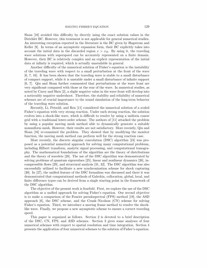
Fig. 3.1. Plot of absolute values of modified wavenumbers versus wavenumber for second deriva-tive approximation.

arbitrary order [27]. For a more detailed Fourier analysis of the numerical resolutionof the DSC algorithm, we refer to [33].

Fourier analysis is a classical technique for comparing different schemes [21]. In-deed, discrete Fourier analysis characterizes the Fourier resolution of an interpolationor differentiation scheme applied to a class of compactly supported and periodic func-tions. Thus, Fourier analysis is capable of providing an effective way to quantify theaccuracy of different approximation schemes used for band-limited periodic functions.It is noted that the outcome of the analysis may not hold when the function is notband limited and periodic.

Because the derivatives are approximated by means of discrete convolution (see(2.8)) in the DSC algorithm, according to the convolution theorem, the corresponding

Fourier coefficients of spatial derivatives can be expressed as u(n)k = δ

(n)α,σ(k)uk, where

δ(n)α,σ(k) = 1

N

∑N−1j=0 δ

(n)α,σ(xj) exp(−iξkxj). Here, by using resolution ∆ = L/N , the

discrete wavenumbers ξk = 2πk/L (k = −N/2 + 1, . . . ,−1, 0, 1, . . . , N/2) range from−π/∆ to π/∆. The quantity π/∆ is the Nyquist frequency, which is the maximumwavenumber that could be distinguished by the discretization with the mesh size ∆.Any wavenumber whose absolute value is greater than the Nyquist frequency will bemisinterpreted and contribute to the aliasing error. For convenience, we introduce ascaled wavenumber ω = 2πk∆/L = 2πk/N and a scaled coordinate s = x/∆. In termsof these new definitions, the Fourier modes are simply exp(−iωx) and the domain ofthe wavenumber ω is [−π, π].

Generally, the derivative approximation of different schemes can be expressed in

the spectral space in a unified form, u(n)k = ω(n)uk. For the second-order derivative,

both the FPS and ASD methods provide the exact response function ω(2) = −ω2

within the frequency band [−π, π]. It is noted that other spectral methods do notprovide exact derivatives with respect to the discrete Fourier analysis. For the DSCand CN schemes, the accuracy of the derivative approximations for band-limited pe-riodic functions can be indicated by the closeness of the modified wavenumber ω(2) to−ω2; see Figure 3.1. It is obvious from Figure 3.1 that the DSC scheme can stay veryclose to the exact differentiation except for very high wavenumbers, while the centralfinite difference used in the CN scheme deviates from the exact second derivative veryquickly.

The analysis indicates that the spectral basis provides the most accurate (i.e.,exact) representation in the Fourier space. However, the same spectral basis is not


the best basis in a finite polynomial space, where the finite difference approximationcan be proved to be the most accurate basis. The analysis also reveals that the DSCalgorithm provides extremely high accuracy comparable to the pseudospectral methodfor approximating band-limited periodic functions. In fact, for problems with someother features, the DSC algorithm can be more accurate than the pseudospectralmethod [33].

3.2. Temporal discretization errors. The standard temporal discretizationsare used for the CN, FPS, and DSC schemes. Thus, it is clear that the temporaldiscretization error is of fourth order for both the FPS and DSC schemes and isO(∆t2) for the CN scheme. The time truncation error for the ASD scheme needs tobe clarified, although it was stated as O(∆t5) [6].

Substitute the initial conditions in (2.15) and (2.16) at time step tm into (2.14),

∆u(xn, tm,∆t) = um+1n − um

n = fm+1n − um

n + gm+1n − um

n .(3.1)

Consequently, we have

um+1n = fm+1

n + gm+1n − um

n .(3.2)

Consider the temporal semidiscretization form of (1.2), i.e., the integral of

um+1n − um

n =

∫ tm+1

tm

∂2u(xn, s)

∂x2ds +

∫ tm+1

tm

u(xn, s)(1 − u(xn, s))ds.(3.3)

Instead of solving (3.3), the ASD scheme actually solves

fm+1n − um

n =

∫ tm+1

tm

∂2f(xn, s)

∂x2ds,(3.4)

gm+1n − um

n =

∫ tm+1

tm

g(xn, s)(1 − g(xn, s))ds.

In terms of the same discrete numerical temporal integration method, (3.3) and (3.4)are equivalent only if the conditions

fm+1n = um+1

n , gm+1n = um+1

n(3.5)

are satisfied simultaneously. This is not true due to (3.2), and these important con-ditions are neglected in the formulation of the ASD scheme. Conditions (3.5) can beapproximately satisfied when ∆t → 0,

fm+1n = um+1

n + O(∆t), gm+1n = um+1

n + O(∆t).(3.6)

Therefore, the temporal truncation error of the ASD scheme is O(∆t). This is verifiedby the numerical experiments reported in the next section.

4. Numerical studies. In the present study, we focus our attention on a par-ticular DSC kernel, the regularized Shannon’s kernel, which has been extensively usedin previous calculations [23, 24, 25, 26, 27, 28, 29, 30, 31, 32, 33]. The DSC param-eters are chosen as W = 32 and σ = 3.5∆ [24]. For the FPS and ASD methods,the computational domain is symmetrically extended so that the periodic BC can beassumed [6]. Thus, for the two spectral methods, when mesh points are reported asN , there are actually 2N grid points used in the computation.


To make a detailed comparison of the DSC, CN, FPS, and ASD methods, sev-eral Cauchy problems of Fisher’s equation, with or without analytical solutions, areemployed. The initial wave profiles studied are all of SSW type. The following SSWsolution is employed in the numerical studies of Li, Petzold, and Ren [11] and Qiuand Sloan [16]:

u(x, t) =

[1 + exp

(√ρ

6x− 5ρ

6t

)]−2

.(4.1)

This traveling wave solution satisfies a scaled Fisher’s equation,

∂u

∂t=

∂2u

∂x2+ ρu(1 − u),(4.2)

and nonlocal conditions (1.3) and (1.4). The speed of the solution (4.1) is c = 5√

ρ/6.For the numerical studies of solution (4.1), the accuracy of the numerical results ismeasured by means of the L∞- and L2-norms. Here L∞ = maxi=1,...,N |ui − ui|and L2 = [ 1

N

∑Ni=1(ui − ui)

2]1/2, where ui and ui are the analytical and numericalsolutions, respectively.

Apart from SSW solution (4.1), other types of SSW profiles are also studied. Forthe purpose of general applications, the difference of the theoretical and numericalwave speed |c − c| is calculated for all studied cases. To estimate the speed of thesimulated traveling wave solution, c, a reference position for the propagating wavefront is introduced, xm

f =∫ xR

xLu(x, tm)dx. This reference position is a simpler ver-

sion of that used by Carey and Shen [2], and the integral is approximated by usingSimpson’s rule. By using this estimate of wave front location, the wave speed may beapproximated as cm = (xm

f − xm−1f )/∆t. Note that the wave speed difference, |c− c|,

can be explained as an approximation error only when the solution reaches the steadystate of the motion.

4.1. Weak reaction problem. We first consider ρ = 1 in solution (4.1); (4.2)then is identical to (1.2). The wave speed of the analytical solution is c = 5

√1/6 ≈

2.04124 > 2. Fisher’s equation is numerically solved via the four methods. Becausethe BC applied on the left-hand boundary is relatively unimportant to the correctnessof the numerical solutions, throughout the present work, the BC on the left is fixedas the Dirichlet BC by setting u(xL, t) = 1 in the DSC and CN schemes. Since theFPS and ASD methods can be used only for periodic BCs, the exact BC (i.e., the BCgiven by the exact solution (4.1)) used in [11, 16] cannot be directly implemented forthe FPS and ASD methods. To achieve a comparison of the four methods, we applythe zero BC (the Dirichlet BC by setting u(xR, t) = 0) at the right-hand boundary inthe DSC and CN schemes.

The numerical results approximated by the four numerical approaches with dif-ferent resolutions are listed in Table 4.1. It can be seen from Table 4.1 that the DSCalgorithm always has accuracy comparable to the FPS method, and both schemesachieve very high accuracy. However, for the ASD method, although highly accuratespatial discretization is used, the approximated results are much less accurate thanthose of the FPS. When ∆t is large, the results of the ASD are even worse than thoseof the CN.

To numerically test the order of accuracy of each scheme with respect to spatialand temporal discretizations, the used resolutions in Table 4.1 are specially designed.A general principle is that, to test the spatial (or temporal) accuracy order, the


Table 4.1Comparison of numerical solution of a scaled Fisher’s equation with ρ = 1 by using the DSC,

CN, FPS, and ASD schemes.

t = 5.0 t = 10.0Scheme N ∆x ∆t L∞ L2 |c− c| L∞ L2 |c− c|

DSC

128 1.0 0.2 1.34(−5) 2.74(−6) 4.25(−5) 5.61(−5) 1.17(−5) 9.15(−5)128 1.0 0.1 9.00(−7) 1.84(−7) 2.95(−6) 3.86(−6) 8.03(−7) 6.41(−6)64 2.0 0.01 4.35(−6) 9.38(−7) 1.34(−7) 3.12(−6) 6.50(−7) 1.19(−7)128 1.0 0.01 1.59(−9) 2.50(−10) 7.02(−9) 1.39(−9) 2.06(−10) 8.43(−10)

CN

512 0.25 0.2 5.18(−3) 1.10(−3) 1.18(−2) 1.43(−2) 2.99(−3) 1.69(−2)512 0.25 0.1 1.35(−3) 2.91(−4) 3.48(−3) 4.25(−3) 8.88(−4) 5.53(−3)64 2.0 0.01 1.02(−2) 1.87(−3) 4.47(−2) 5.47(−2) 1.16(−2) 1.04(−1)128 1.0 0.01 2.66(−3) 4.84(−4) 1.15(−2) 1.46(−2) 3.06(−3) 2.77(−2)

FPS

128 1.0 0.2 1.34(−5) 2.74(−6) 4.25(−5) 5.61(−5) 1.17(−5) 9.15(−5)128 1.0 0.1 9.01(−7) 1.84(−7) 2.94(−6) 3.86(−6) 8.03(−7) 6.41(−6)64 2.0 0.01 3.16(−6) 6.75(−7) 6.89(−8) 3.21(−6) 6.76(−7) 1.10(−7)128 1.0 0.01 1.27(−9) 1.38(−10) 4.01(−9) 4.40(−10) 8.78(−11) 7.58(−10)

ASD

128 1.0 0.2 3.84(−2) 7.24(−3) 9.38(−2) 1.09(−1) 2.19(−2) 1.26(−1)128 1.0 0.1 1.96(−2) 3.73(−3) 4.93(−2) 5.62(−2) 1.14(−2) 6.68(−2)64 2.0 0.01 1.99(−3) 3.83(−4) 5.16(−3) 5.67(−3) 1.18(−3) 7.06(−3)128 1.0 0.01 1.99(−3) 3.83(−4) 5.16(−3) 5.72(−3) 1.18(−3) 7.06(−3)

Table 4.2Numerically tested accuracy order of the four methods.

t = 5.0 t = 10.0Halve DSC CN FPS ASD DSC CN FPS ASD∆t 3.89 1.92 3.89 0.96 3.86 1.75 3.86 0.94∆x 11.87 1.95 12.26 3.77(−5) 11.62 1.92 12.91 1.22(−4)

temporal (spatial) resolution will be chosen as sufficiently fine and kept unchanged,while the spatial (temporal) resolution will be halved. The principle is easily satisfiedfor testing spatial accuracy by setting ∆t = 0.01 and halving ∆x = 2.0 to 1.0. Fortesting temporal accuracy, however, ∆x could not be too small, because usually thereis a stability constraint for the mesh ratio ∆t/∆x2 for explicit schemes. Fortunately,the spatial discretization accuracy of three explicit schemes, the DSC, the FPS, andthe ASD, is very high such that ∆x = 1.0 is enough in the present study to guaranteethat the approximation errors are mainly contributed by the temporal discretization.For the low spatial accuracy scheme, the CN, ∆x is set to ∆x = 0.25, since the CNscheme is unconditionally stable.

In terms of the L2 errors, the error decreasing rates of each scheme are re-calculated from Table 4.1 and are presented in Table 4.2. The numerically estimatedaccuracy orders are all in excellent agreement with the theoretical analyses in section3. When ∆x is halved, the DSC results become over 3000 times more accurate thanthe original ones, and the accuracy increasing rates of the FPS are even larger than4000. The numerical results indicate that the spatial accuracy orders of these twoschemes are extremely high. The temporal discretization orders of both the DSC andFPS schemes are approximately O(∆t4), since the same RK4 scheme is used in bothschemes. The numerically tested truncation errors of the CN scheme are also in agree-ment with the classic theoretical analysis, i.e., O(∆x2) and O(∆t2). It is interestingto note that by halving ∆x, the accuracy of the ASD results remains unchanged;this means that the approximation errors of the ASD scheme are fully introduced bytemporal discretization. By halving ∆t, the accuracy of the ASD results increasesapproximately two times; therefore, the temporal truncation error of the ASD scheme


−0.2 0 0.2 0.4 0.6 0.80

0.2

0.4

0.6

0.8

1(a)

x

u

−0.2 0 0.2 0.4 0.6 0.80

0.2

0.4

0.6

0.8

1(b)

x

u−0.2 0 0.2 0.4 0.6 0.80

0.2

0.4

0.6

0.8

1(c)

x

u

−0.2 0 0.2 0.4 0.6 0.80

0.2

0.4

0.6

0.8

1(d)

xu

Fig. 4.1. Numerical solutions of a scaled Fisher’s equation with ρ = 104 at times t = 5.0(−4),1.0(−3), . . . , 2.5(−3). (a) The DSC solutions; (b) the CN solutions; (c) the FPS solutions; (d)the ASD solutions. In all charts, the continuous lines represent the analytical solutions at thecorresponding times.

is O(∆t). This verifies the earlier analysis.

4.2. Strong reaction problem. The strong reaction problem, ρ = 104, is con-sidered for the scaled Fisher’s equation (4.2). The wave speed of the analytical solu-tion is c = 5

√104/6 ≈ 204.124. It is noted that this wave speed is in terms of the

unnormalized coordinate system. The corresponding minimum wave speed is c = 200.

4.2.1. Shock-like wave. With the strong reaction force, the solution evolvesinto a shock-like wave. Thus, in order to properly represent the rapidly changingsolution by a low-order scheme, very fine resolution has to be used. To avoid theburden of using a large computation grid, a nonuniform mesh is conventionally used.Li, Petzold, and Ren [11] and Qiu and Sloan [16] considered this strong reactionproblem by using the moving mesh methods, which are able to redistribute grid pointsto follow a rapidly changing solution. Satisfactory results were obtained in [16].

In the present study, we consider a uniform mesh to solve this strong reactionproblem. Following the discrete Fourier analysis in section 3, higher-order schemesare much better in resolving a higher wavenumber, with the same spacing ∆x. There-fore, an accurate result could be obtained by using higher-order schemes with smallN . To illustrate this argument, the solution of Fisher’s equation with ρ = 104 isapproximated by the DSC, CN, FPS, and ASD schemes. The zero BC is used in boththe DSC and CN schemes. Discretization parameters used here are similar to thoseof [16]: N = 64, ∆x = 0.02, and ∆t = 5.0(−6). The computation domain is fixed as[xL, xR] = [−0.2, 1.06]. Note that the present mesh resolution is equal to the averagemesh resolution used in [16]. The present numerical results are shown in Figure 4.1and Table 4.3. It can be seen from Table 4.3 that the results of moving mesh methodsare much more accurate than those of the convention finite difference scheme, whilethe results of higher-order schemes, i.e., the FPS and DSC, are in turn much moreaccurate than those in [16]. However, for the FPS scheme, although a very accurateresult is obtained up to t = 2.5(−3), it blows up at t = 4.0(−3).

As noticed by some researchers [6, 20, 2] in the literature, spectral methods gener-ate unwanted oscillations at the wave front, and since the solution of Fisher’s equation


Table 4.3Comparison of short-term solution of a scaled Fisher’s equation with ρ = 104 approximated by

the DSC, CN, FPS, and ASD schemes and by moving mesh methods. Three results from Qiu andSloan [16] are listed. (a) MMDAE with N = 50; (b) MMPDE 6 with N = 50 and τ = 10−7; (c)method of lines on an evenly spaced grid with N = 300.

tScheme Error 5.0(−4) 1.0(−3) 1.5(−3) 2.0(−3) 2.5(−3) 3.0(−3) 3.5(−3) 4.0(−3)

DSC

L∞ 6.28(−6) 3.03(−6) 1.98(−6) 3.23(−6) 4.46(−6) 5.44(−6) 6.22(−6) 1.69(−5)L2 1.24(−6) 6.53(−7) 5.92(−7) 8.35(−7) 1.16(−6) 1.43(−6) 1.64(−6) 4.30(−6)|c− c| 2.53(−3) 1.06(−4) 6.23(−5) 6.58(−5) 7.37(−5) 1.00(−4) 5.19(−4) 1.57(−2)

CN

L∞ 1.03(−2) 5.55(−2) 1.25(−1) 2.04(−1) 2.80(−1) 3.60(−1) 4.48(−1) 5.21(−1)L2 1.92(−3) 1.17(−2) 2.65(−2) 4.36(−2) 6.18(−2) 8.04(−2) 9.91(−2) 1.17(−1)|c− c| 4.49(+0) 1.04(+1) 1.31(+1) 1.46(+1) 1.54(+1) 1.60(+1) 1.64(+1) 1.67(+1)

FPS

L∞ 3.13(−6) 3.47(−6) 3.90(−6) 5.00(−6) 7.82(−5) 4.23(−3) 3.42(−1) ∞L2 7.71(−7) 6.79(−7) 7.02(−7) 9.04(−7) 2.11(−5) 1.19(−3) 8.95(−2) ∞|c− c| 1.58(−3) 7.72(−5) 9.73(−5) 1.87(−3) 9.68(−2) 5.54(+0) 4.76(+2) ∞

ASD

L∞ 1.07(−2) 2.88(−2) 4.93(−2) 7.10(−2) 9.37(−2) 1.24(−1) 9.44(−1) ∞L2 2.09(−3) 6.07(−3) 1.06(−2) 1.53(−2) 2.02(−2) 2.68(−2) 2.35(−1) ∞|c− c| 2.61(+0) 3.45(+0) 3.70(+0) 3.80(+0) 4.05(+0) 1.59(+1) 3.41(+2) ∞

[16] (a) L∞ 9.25(−3)[16] (b) L∞ 4.29(−2)[16] (c) L∞ 9.34(−3)

0 5 10 15 20

0

5

10

15

20x 10

−15 (a)

x

u

0 5 10 15 20

0

5

10

15

20x 10

−15 (b)

x

u

Fig. 4.2. The plots of the front parts of the wave solutions approximated by the FPS and ASDschemes at time t = 1∆t. (a) The FPS solution; (b) the ASD solution.

is unstable to the small perturbation at the wave front, the results of spectral methodsquickly become unstable. In the present studies, it is found that the serious oscilla-tions are generated in both the FPS and ASD solutions even after only one timeintegration (see Figure 4.2), while the DSC and CN results are free of these oscilla-tions. To ensure the stability, Gazdag and Canosa [6] suggested using an additionalprocedure to suppress the oscillations at each time step; i.e., if u(xn, tm) ≤ ε, thenu(xn, tm) = 0. Here the threshold ε is a small positive number and is chosen empiri-cally. Note that by adopting this suppression procedure, it is equivalent to imposingthe zero BC at xR(tm).

4.2.2. The moving frame method. In order to simulate the long-time behav-ior of the traveling wave solutions, the computational domain has to be very largedue to the high wave speed. At the same time, a relatively fine spatial resolutionis required to properly represent the wave solution of this strong reaction problem.Therefore, the computational cost will be extremely expensive, as much computa-tion is wasted on unimportant regions. To reduce the computational cost, a movingcoordinate system with user-specified speed was introduced by Hagstrom and Keller[8]: at each instant, the computation is focused only on a narrow region within theframe. However, this technique could not be directly applied to general cases since,


x ( )tmLx ( )tmt0( )Rxt0( )Lx R

Grid support of the moving frame

tmu(x, )u(x, )t0

1

u

0

x

Fig. 4.3. The schematic plot of the moving frame coordinate.

in practice, the speed of the moving coordinate system may not be known a priori.To account for wide applications, a moving frame method is introduced in the

present study. The method provides grid support only to the region of interest. Thecenter of the moving frame goes along with the center of the traveling wave. As such,the moving frame method dramatically reduces the computational grid size. To thisend, we introduce a monitor function

M(x, t) =√

φ2 + ψ2(∂u(x, t)/∂x)2.(4.3)

Monitor function (4.3) can be viewed as a generalization of the arc-length monitorfunction, which is widely used in moving mesh methods [11, 16]. Then the centralpoint of the traveling wave solution can be identified by means of the monitor function(4.3), xm

c = maxn=1,2,...,N M(xn, tm). In the numerical study, the initial computationdomain, [xL(t0), xR(t0)], is first selected and the initial wave center, x0

c , is calculated.Then the computational domain will move according to the corresponding wave center,i.e., xL(tm) = xL(t0) + (xm

c − x0c), and xR(tm) = xR(t0) + (xm

c − x0c), at each time

step tm. It is noted that the objectives of the present moving frame method andthe previous moving mesh method [11, 16] are different; e.g., the former moves thecoordinate system to follow up a rapidly traveling solution (see Figure 4.3), while thelatter seeks a redistribution of grid points to catch up with a rapidly changing solutionwithin a fixed coordinate system. A uniform mesh with a fixed resolution is used inthe moving frame method. If xR(tm) > xR(tm−1), then u(xR(tm), tm) will be givenby the BC applied on xR(tm). In the present study, for simplicity we choose φ = 0and ψ = 1, although φ = 1 could also be utilized.

In association with the moving frame method, the medium-term solutions of thescaled Fisher’s equation are approximated by the four methods. For all four methods,the spatial discretization parameters are fixed as N = 512 and ∆x = 8.5(−3), and thetime increment is set to ∆t = 5.0(−6). The zero BC is applied at the right boundary inthe DSC and CN schemes; the empirically optimal threshold is chosen to suppress theoscillations in two spectral methods. The numerical results are presented in Table 4.4.It can be seen from Table 4.4 that the steady states of motion are reached for thenumerical solutions of the CN, FPS, and ASD methods. The asymptotic velocities ofthese solutions are all incorrect. The steady state wave speed of the FPS results isc = 199.5 ≈ 200, which is close to the expectation of the theoretical analysis while,for two low accuracy methods (the CN and ASD), the asymptotic velocities havevery large errors. The wave speed estimated by the FPS and ASD methods withoptimal suppression is shown in Figure 4.4. The results of the DSC approach are


Table 4.4Comparison of medium-term solution of a scaled Fisher’s equation with ρ = 104 approximated

by the DSC, CN, FPS, and ASD schemes.

tScheme Error 0.02 0.04 0.06 0.08 0.10 0.12

DSC, zero BCL∞ 1.74(−5) 3.57(−5) 6.21(−5) 1.57(−2) 2.07(−1) 7.66(−1)L2 1.97(−6) 4.07(−6) 7.05(−6) 1.78(−3) 2.36(−2) 9.94(−2)|c− c| 7.70(−5) 7.72(−5) 4.84(−4) 2.66(−1) 1.40(+0) 1.62(+1)

CN, zero BCL∞ 6.54(−1) 9.30(−1) 9.88(−1) 9.98(−1) 1.00(+0) 1.00(+0)L2 8.23(−2) 1.46(−1) 1.93(−1) 2.30(−1) 2.62(−1) 2.88(−1)|c− c| 3.45(+0) 3.45(+0) 3.45(+0) 3.45(+0) 3.31(+0) 2.95(+0)

CN, exact BCL∞ 6.54(−1) 9.30(−1) 9.88(−1) 9.98(−1) 1.00(+0) 1.00(+0)L2 8.23(−2) 1.46(−1) 1.93(−1) 2.30(−1) 2.62(−1) 2.89(−1)|c− c| 3.45(+0) 3.45(+0) 3.45(+0) 3.45(+0) 3.35(+0) 3.02(+0)

CN, asymptotic BCL∞ 6.54(−1) 9.30(−1) 9.88(−1) 9.98(−1) 1.00(+0) 1.00(+0)L2 8.23(−2) 1.46(−1) 1.93(−1) 2.30(−1) 2.62(−1) 2.89(−1)|c− c| 3.45(+0) 3.45(+0) 3.45(+0) 3.45(+0) 3.35(+0) 3.02(+0)

FPS, ε = 1.0(−14)L∞ 6.75(−1) 9.64(−1) 9.97(−1) 9.99(−1) 1.00(+0) 1.00(+0)L2 8.46(−2) 1.64(−1) 2.19(−1) 2.63(−1) 3.00(−1) 3.33(−1)|c− c| 4.57(+0) 4.58(+0) 4.58(+0) 4.58(+0) 4.58(+0) 4.58(+0)

ASD, ε = 1.5(−14)L∞ 9.58(−1) 9.99(−1) 1.00(+0) 1.00(+0) 1.00(+0) 1.00(+0)L2 1.59(−1) 2.55(−1) 3.24(−1) 3.80(−1) 4.29(−1) 4.73(−1)|c− c| 8.62(+0) 8.66(+0) 8.65(+0) 8.65(+0) 8.65(+0) 8.65(+0)

0 0.01 0.02 0.03 0.04 0.05

192

196

200

204

208 CN

DSC

FPS

ASD

time

Wav

e sp

eed

Fig. 4.4. The plots of the wave speed estimated by four methods for the strong reaction problem.

more accurate than others, as shown in Table 4.4. However, the final DSC results arealso relatively inaccurate, which is due to the improper BC.

4.2.3. A new asymptotic scheme. Apart from the exact BC, the only properBC reported in the literature is the one given by Hagstrom and Keller [8]. In thepresent study, however, their BC is relatively complicated to implement. Therefore,a simple asymptotic BC is introduced that is based on a consideration similar to thatin [8]. By assuming that the solution at the boundary cutoff is sufficiently close toits limiting value, an asymptotic representation of the initial data in the discardedregion can be simply expressed as

u0(x) = a exp(−bx), x ≥ xR(t0),(4.4)

for some constants a and b. When x is sufficiently large, the finite sum of exponentialsfor the initial data used in [8] can be well approximated by (4.4). Furthermore, whenx → ∞, b will tend to β. Without cumbersome construction, the asymptotic BCutilized in the present work is assumed to have the form

u(x, tm) = a exp(−b(x− ctm)), x ≥ xR(tm),(4.5)


Table 4.5Long-term solution of a scaled Fisher’s equation with ρ = 104 approximated by the DSC scheme.

DSC, exact BC DSC, asymptotic BCt L∞ L2 |c− c| L∞ L2 |c− c|0.02 1.74(−5) 1.97(−6) 7.70(−5) 1.74(−5) 1.97(−6) 7.70(−5)0.04 3.57(−5) 4.07(−6) 7.72(−5) 3.57(−5) 4.07(−6) 7.72(−5)0.06 5.43(−5) 6.16(−6) 7.71(−5) 5.43(−5) 6.16(−6) 7.71(−5)0.08 4.05(−5) 4.59(−6) 5.68(−4) 4.05(−5) 4.59(−6) 5.68(−4)0.10 3.11(−4) 3.53(−5) 1.53(−3) 3.11(−4) 3.53(−5) 1.53(−3)0.20 4.84(−4) 5.49(−5) 3.12(−5) 4.84(−4) 5.49(−5) 3.12(−5)0.30 4.87(−4) 5.53(−5) 3.69(−5) 4.87(−4) 5.53(−5) 3.69(−5)0.40 4.90(−4) 5.57(−5) 3.81(−5) 4.90(−4) 5.57(−5) 3.81(−5)0.50 4.94(−4) 5.60(−5) 1.31(−5) 4.94(−4) 5.60(−5) 1.31(−5)0.60 4.91(−4) 5.60(−5) 1.09(−5) 4.91(−4) 5.60(−5) 1.09(−5)0.70 4.92(−4) 5.57(−5) 2.22(−5) 4.92(−4) 5.57(−5) 2.22(−5)0.80 4.94(−4) 5.65(−5) 3.68(−5) 4.94(−4) 5.65(−5) 3.68(−5)0.90 4.89(−4) 5.54(−5) 1.17(−5) 4.89(−4) 5.54(−5) 1.17(−5)1.00 4.88(−4) 5.57(−5) 2.99(−5) 4.88(−4) 5.57(−5) 2.99(−5)

for each time step tm. Unlike the BC in [8], where the asymptotic expansion isassumed to be known, here the constants a, b, and c are estimated from initial dataat the boundary cutoff xN = xR(t0),

a =u0(xN )

exp (−xN ln(u0(xN−1)/u0(xN ))/∆x),

b = ln(u0(xN−1)/u0(xN ))/∆x,(4.6)

c =

{b + 1

b, b ≤ 1,

2, b ≥ 1.(4.7)

In other words, the asymptotic BC is self-contained in our numerical algorithm; noadditional knowledge about the initial data is requested in advance. Therefore, theadvantages of the present asymptotic BC are that it is simple, fully automatic, andsuitable for general applications.

By using the asymptotic and exact BCs at x = xR, the long-term solutions ofFisher’s equation are approximated via the DSC algorithm; see Table 4.5. It is obviousthat the asymptotic BC results are the same as those of the exact BC, which meansthat the proposed asymptotic BC approximates the exact BC extremely well. Thesteady state solutions are reached at t = 0.2; the final DSC results are very accurateat t = 1.0. In fact, similarly accurate results can be obtained no matter how larget is. The asymptotic and exact BCs can be implemented with the CN scheme; thecorresponding results are contained in Table 4.4. However, no improvement is madein the CN results by using either the asymptotic or exact BC. The uselessness ofthe asymptotic and exact BCs here is due to the low accuracy of the CN schemefor this problem. The wave speeds estimated by the DSC and CN schemes with theasymptotic BC are depicted in Figure 4.4.

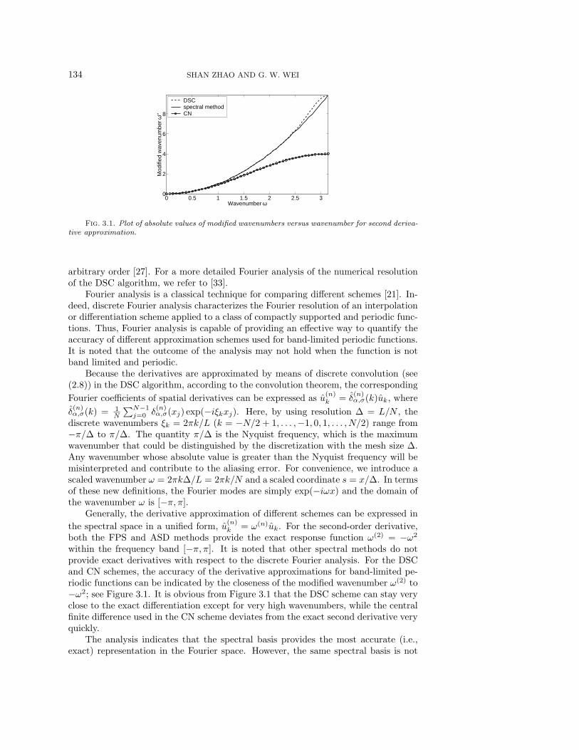
Therefore, apart from the appropriate BC, the accuracy of the scheme is also acrucial factor for producing correct results. For the strong reaction problem, only thehighly accurate DSC schemes can give the results as predicted by theoretical analysis;see Figure 4.5. It can be seen from Figure 4.5 that the wave solution of the FPShas a speed of c ≈ 200. The importance of the moving frame method is also clearly


2 4 6 8 10 12 14 16 18 20 220

0.2

0.4

0.6

0.8

1

(a)

x

u

2 4 6 8 10 12 14 16 18 20 220

0.2

0.4

0.6

0.8

1

(b)

x

u

Fig. 4.5. Numerical solutions of a scaled Fisher’s equation with ρ = 104 at times t = 0.01,0.02, . . . , 0.1. (a) The DSC solutions; (b) the FPS solutions. In both charts, the continuous linesrepresent the analytical solutions at the corresponding times.

illustrated in Figure 4.5. It is seen that the frame moves consistently according to thesimulated wave speed and, at each instant, the computational domain is very narrowcompared with the whole occupied physical domain.

4.3. SSW simulation study. In this subsection, we study further the sensi-tivity of the simulated speed of the traveling wave to the proper BCs. In additionto the wave solution (4.1), there are other kinds of SSW solutions studied in the lit-erature [1, 6, 8, 2]. Since Hagstrom and Keller did not explicitly report their initialwave profiles, the only available example of an initial SSW profile is the one givenby Canosa [1], which was also considered by other authors [6, 2]. Unfortunately, asreported by Carey and Shen [2], a slight negative undershoot appears in the initialprofile of such an SSW so that a noticeably negative undershoot will be developed inthe computation. Carey and Shen suggest forcing the negative u to zero in the initialprofile. However, by doing so, the initial wave profile will evolve into a minimumspeed wave.

In the present study, the dimensionless Fisher’s equation (1.2) is considered andseveral SSW profiles are simply generated by the initial function

u0(x) = [1 + exp(b1x) + exp(b2x)]−1

,(4.8)

where 0 ≤ b1 < 1 and 0 ≤ b2 < 1. Three sets of parameters are tested: b1 = 0.5 andb2 = 0; b1 = 0 and b2 = 0.25; and b1 = 0.5 and b2 = 0.25. The corresponding SSWsare denoted SSW1, SSW2, and SSW3, respectively. The steady state wave speeds ofSSW1, SSW2, and SSW3 are c = 2.5, c = 4.25, and c = 2.5, respectively. In theSSW3, the initial profile is given by the combination of two exponentials. Thus, as ageneral case, SSW3 is a good test problem for investigating the performance of theproposed asymptotic BC.

Taking N = 256, ∆x = 1.0, and ∆t = 0.1, the proposed asymptotic BC isimplemented in both the DSC and CN schemes, while the optimal suppression isemployed in both the FPS and ASD methods. To simulate a long-term solution,the proposed moving frame method is utilized. The numerical solutions of Fisher’sequation approximated by the four methods are shown in Table 4.6 and the simulated


Table 4.6The errors of the wave solution speed (|c− c|) estimated by the DSC, CN, FPS (ε = 2.0(−12)),

and ASD (ε = 1.0(−11)) schemes.

t = 100 t = 200 t = 300 t = 400 t = 500

SSW1

DSC 1.76(−3) 9.49(−7) 5.68(−13) 2.84(−13) 0.0CN 4.75(−3) 8.72(−6) 6.49(−7) 1.42(−12) 8.52(−13)FPS 5.12(−1) 5.13(−1) 5.13(−1) 5.13(−1) 5.13(−1)ASD 5.94(−1) 5.86(−1) 5.88(−1) 5.88(−1) 5.88(−1)

SSW2

DSC 1.00(−8) 1.01(−8) 1.01(−8) 1.01(−8) 1.01(−8)CN 7.43(−9) 7.43(−9) 7.43(−9) 7.43(−9) 7.43(−9)FPS 2.26(+0) 2.26(+0) 2.26(+0) 2.26(+0) 2.26(+0)ASD 2.34(+0) 2.33(+0) 2.33(+0) 2.33(+0) 2.33(+0)

SSW3

DSC 1.56(−3) 8.77(−6) 8.52(−13) 2.84(−13) 0.0CN 5.78(−3) 9.59(−5) 9.94(−13) 2.84(−13) 2.84(−13)FPS 5.12(−1) 5.13(−1) 5.13(−1) 5.13(−1) 5.13(−1)ASD 5.94(−1) 5.86(−1) 5.87(−1) 5.88(−1) 5.88(−1)

20 40 60 80 1001

1.5

2

2.5

3

(a)

time

Wav

e sp

eed

CN DSCFPSASD

20 40 60 80 100

0.5

1.25

2

2.75

3.5

4.25

5

(b)

time

Wav

e sp

eed

CN DSCFPSASD

20 40 60 80 100

1.75

2

2.25

2.5

2.75(c)

time

Wav

e sp

eed

CN DSCFPSASD

Fig. 4.6. The plots of the wave speed estimated by the four methods for SSWs. (a) SSW1; (b)SSW2; (c) SSW3.

wave speeds of the four methods are displayed in Figure 4.6. All numerical resultsare in excellent agreement with the theoretical analysis. The simulated wave speedof two spectral methods evolves gradually to the minimum speed c = 2, due to thesuppression. The FPS results are relatively closer to theoretical value than those ofthe ASD method. By using the asymptotic BC, both the DSC and the CN generatesimilarly excellent results. When t < 300, the DSC results are more accurate thanthose of the CN method; when t > 300, the differences between the results of twoschemes are negligible. Compared with the results obtained by the CN scheme for thestrong reaction problem, the poor results obtained there are due to the low accuracyof the CN scheme. For the present case, the resolution of the CN scheme is sufficientto resolve the solutions. Thus, by using the asymptotic BC, excellent asymptoticsolutions are obtained. In SSW3, amazingly accurate results are also achieved as inSSW1, which demonstrates the usefulness of the proposed simple asymptotic BC forthe general applications. The only difference in the wave speeds of SSW1 and SSW3is the starting wave speed; see Figure 4.6.

5. Conclusion. This paper explores the utility of the discrete singular convolu-tion (DSC) algorithm for solving Fisher’s equation. Several numerical issues that arecrucial to the long-time behavior of the numerical solution of Fisher’s equation aresuccessfully treated in the present work. An accurate, robust, and efficient algorithmis constructed that yields sound simulation of the steady state of the equation. Tofurther evaluate the present algorithm, three other standard methods are employedfor a comparison. Fourier analysis is utilized to assess the spatial resolution of the four


methods. The temporal truncation orders of the four methods are clarified. Extensivenumerical experiments are carried out to verify the theoretical analysis and to com-pare the accuracy, stability, flexibility, and efficiency of the four numerical schemes.Superspeed wave (SSW), which is numerically difficult, is chosen in the present study.All numerical results are validated either by analytical solutions or by the steady statewave speed.

Several interesting numerical issues of Fisher’s equation are elaborated on in thepresent work. First, with strong reaction, the solution will evolve into a shock-likewave, which usually leads to inaccurate approximation. The numerical approximationcould be greatly improved if a nonuniform moving mesh were used [16]. In the presentstudy, it is demonstrated that, without utilizing a nonuniform mesh, the DSC andFourier pseudospectral (FPS) schemes can produce much better results than those of[16]. This suggests that the high accuracy scheme could be a better way to resolveshock-like wave. Second, a moving frame method, which can automatically trackthe traveling wave, is introduced in the present work. This novel method provides anefficient and computationally feasible way to study long-time traveling wave solutions.Third, the SSW solution of Fisher’s equation will quickly evolve into the minimumspeed wave if an improper BC is applied at the right-hand boundary. Unfortunately,the only appropriate BC reported in the literature [8] requires a priori knowledge of theinitial data, so it is not computationally applicable in general situations. To overcomethis critical difficulty, a simple asymptotic scheme is proposed in the present work thatis fully automatic and suitable for general applications. Numerical studies on threekinds of SSWs demonstrate the success of this new asymptotic scheme. Finally, withthe new asymptotic scheme and moving frame method, the resulting DSC algorithm isshown to be an accurate, reliable, and efficient approach for solving Fisher’s equation.

To further illustrate the performance of the DSC algorithm, three standard meth-ods are employed to make a comparison for solving Fisher’s equation. Based on thisstudy, the following remarks can be made about these four methods:

1. The Fourier analysis indicates that the DSC scheme can provide spectral-likeresolution over a broad range of wavenumbers. Comparable high accuracy isobtained in the numerical results of both the FPS and DSC schemes. TheASD scheme has limited accuracy because its temporal discretization is ofO(∆t), instead of O(∆t5) as claimed in the original work [6].

2. The DSC is as flexible in handling complex geometries and BCs as the CN,whereas the two spectral methods are restricted to the periodic BC only.This inflexibility hinders the performance of two spectral methods for solvingFisher’s equation because a correct numerical solution can only be achievedwith appropriate BCs.

3. Undesirable oscillations are generated at the wave front in the numericalsolutions approximated by the two spectral methods [6, 20, 2], and thus thesesolutions quickly become unstable. Such oscillations do not occur in thesolutions of both the DSC and CN.

4. For a small number of grid points N , the DSC scheme usually requires moreCPU time than the two spectral methods. However, when a large N is usedin the strong reaction problem, the required CPU time of the FPS is longerthan that of the DSC.

In summary, in terms of accuracy, flexibility, stability, and efficiency, the DSCalgorithm performs well compared with other existing standard numerical methodsfor the solution of Fisher’s equation.


REFERENCES

[1] J. Canosa, On a nonlinear diffusion equation describing population growth, IBM J. Res. De-velop., 17 (1973), pp. 307–313.

[2] G. F. Carey and Y. Shen, Least-squares finite element approximation of Fisher’s reaction-diffusion equation, Numer. Methods Partial Differential Equations, 11 (1995), pp. 175–186.

[3] R. A. Fisher, The wave of advantage of advantageous genes, Ann. Eugenics, 7 (1937), pp.355–369.

[4] B. Fornberg, On a Fourier method for the integration of hyperbolic equations, SIAM J. Numer.Anal., 12 (1975), pp. 509–528.

[5] B. Fornberg, The pseudospectral method: Comparisons with finite differences for the elasticwave equation, Geophysics, 52 (1987), pp. 483–501.

[6] J. Gazdag and J. Canosa, Numerical solution of Fisher’s equation, J. Appl. Probab., 11(1974), pp. 445–457.

[7] P. S. Hagan, Traveling wave and multiple traveling wave solutions of parabolic equations,SIAM J. Math. Anal., 13 (1982), pp. 717–738.

[8] T. Hagstrom and H. B. Keller, The numerical calculation of traveling wave solutions ofnonlinear parabolic equations, SIAM J. Sci. Stat. Comput., 7 (1986), pp. 978–988.

[9] A. Kolmogorov, I. Petrovshy, and N. Piscounoff, Etude de l’equation de la diffusion aveccroissance de la quantite de matiere et son application a un probleme biologique, Bull.Univ. Etat Moscou Ser. Int. Sect. A Math. et Mecan., 1 (1937), pp. 1–25.

[10] D. A. Larson, Transient bounds and time-asymptotic behavior of solutions to nonlinear equa-tions of Fisher type, SIAM J. Appl. Math., 34 (1978), pp. 93–103.

[11] S. Li, L. R. Petzold, and Y. Ren, Stability of moving mesh systems of partial differentialequations, SIAM J. Sci. Comput., 20 (1998), pp. 719–738.

[12] T. Mavoungou and Y. Cherruault, Numerical study of Fisher’s equation by Adomian’smethod, Math. Comput. Modelling, 19 (1994), pp. 89–95.

[13] R. E. Mickens, A best finite-difference scheme for the Fisher equation, Numer. Methods PartialDifferential Equations, 10 (1994), pp. 581–585.

[14] R. E. Mickens, Relation between the time and space step-sizes in nonstandard finite-differenceschemes for the Fisher equation, Numer. Methods Partial Differential Equations, 13 (1997),pp. 51–55.

[15] N. Parekh and S. Puri, A new numerical scheme for the Fisher equation, J. Phys. A, 23(1990), pp. L1085–L1091.

[16] Y. Qiu and D. M. Sloan, Numerical solution of Fisher’s equation using a moving meshmethod, J. Comput. Phys., 146 (1998), pp. 726–746.

[17] Rizwan-uddin, Comparison of the nodal integral method and nonstandard finite-differenceschemes for the Fisher equation, SIAM J. Sci. Comput., 22 (2001), pp. 1926–1942.

[18] J. Roessler and H. Hussner, Numerical solution of the (1+2)-dimensional Fisher’s equationby finite elements and the Galerkin method, Math. Comput. Modelling, 25 (1997), pp. 57–67.

[19] B. F. Sanders, N. K. Katopodes, and J. P. Boyd, Spectral modeling of nonlinear dispersivewaves, J. Hydraulic Engrg., 124 (1998), pp. 2–12.

[20] S. Tang and R. O. Weber, Numerical study of Fisher’s equation by a Petrov-Galerkin finiteelement method, J. Austral. Math. Soc. Ser. B, 33 (1991), pp. 27–38.

[21] R. Vichnevetsky and J. B. Bowles, Fourier Analysis of Numerical Approximations of Hy-perbolic Equations, SIAM, Philadelphia, 1982.

[22] Y. G. Wang, E. H. Twizell, and W. G. Price, Second-order, numerical methods for thesolution of equations in population modelling, Comm. Appl. Numer. Methods, 8 (1992),pp. 511–518.

[23] G. W. Wei, Quasi-wavelets and quasi interpolating wavelets, Chem. Phys. Lett., 296 (1998),pp. 215–222.

[24] G. W. Wei, Discrete singular convolution for the solution of the Fokker-Planck equation,J. Chem. Phys., 110 (1999), pp. 8930–8942.

[25] G. W. Wei, Solving quantum eigenvalue problems by discrete singular convolution, J. Phys.B, 33 (2000), pp. 343–352.

[26] G. W. Wei, Discrete singular convolution for the sine-Gordon equation, Phys. D, 137 (2000),pp. 247–259.

[27] G. W. Wei, A unified approach for the solution of the Fokker–Planck equation, J. Phys. A, 33(2000), pp. 4935–4953.

[28] G. W. Wei, Wavelets generated by using discrete singular convolution kernels, J. Phys. A, 33(2000), pp. 8577–8596.


[29] G. W. Wei, A new algorithm for solving some mechanical problems, Comput. Methods Appl.Mech. Engrg., 190 (2001), pp. 2017–2030.

[30] G. W. Wei, Synchronization of single-side averaged coupling and its application to shock cap-turing, Phys. Rev. Lett., 86 (2001), p. 3542–3546.

[31] G. W. Wei, Vibration analysis by discrete singular convolution, J. Sound Vibration, 244 (2001),pp. 535–553.

[32] G. W. Wei, Discrete singular convolution for beam analysis, Engrg. Structures, 23 (2001),pp. 1045–1053.

[33] S. Y. Yang, Y. C. Zhou, and G. W. Wei, Comparison of the discrete singular convolutionalgorithm and the Fourier pseudospectral method for solving partial differential equations,Comput. Phys. Comm., 143 (2002), pp. 113–135.

Documents

COMPARISON OF THE DISCRETE SINGULAR CONVOLUTION