Comparison of Systematic and RandomSampling for Estimating the Accuracy of MapsGenerated from Remotely Sensed DataStephen V. StehmanSUNY College of Environmental Science and Foresty, 211 Marshall Hall, 1 Forestry Drive, Syracuse, NY 13210

ABST.~a:: Properties of statistical analyses of error matrices generated for accuracy assessment of remote sensingclassificatio~s were evaluated for ~hree sampling designs: systematic, stratified systematic unaligned, and simple ran­dom sampli~~ (SRS). The population parameters investigated were the proportion of rnisclassified pixels, P, and theKappa coeffiCIent o~ agreement, K. Systematic designs were generally more precise than SRS for the populations studied,~cept whe~ ~ampling in phase ~th pe.riodicity in a population. Bias of the estimated proportio~ of rnisclassified pixels,P, wa~ negligible for.the syst~matic deSigns. The common practice of estimating the variance of P for systematic designsby us~g a~ SRS vanance estimator resulted in over- or underestimation of variance, depending on whether the sys­tematic deSign was more or less precise than SRS. A small simulation study showed that the usual standard errorformula for the estimated Kappa coefficient of agreement can perform poorly for systematic designs.

INTRODUCTION

L AND-USE AND LAND-COVER CLASSIFICATION MAPS generatedfrom remote sensing data are valuable management and

planning tools, and the importance of assessing the accuracy ofland-use and land-cover classifications from remotely senseddata has long been recognized. Reference data are needed toproperly assess the accuracy of classifications obtained by re­mote sensing, and obtaining these data by a statistically validsampling design provides the mathematical foundation for sci­entifically rigorous inferences. Reference data are typically usedfor estimating the overall classification accuracy of the map orthe accuracy of individual map categories. Reference data arealso u~ed to construct error matrices, and these matrices maybe subjected to further analyses, such as comparison of differentalgorithms used to create classification maps.

Congalton (1988) and Maling (1989) review recommendationson choice of sampling design for accuracy assessment. Manypapers focus on hypothesis testing to decide whether or notthe map is of acceptable accuracy (Hord and Brooner, 1976;Hay, 1979; Van Genderen et al., 1978; Aronoff, 1982a; Aronoff,1982b). The hypothesis tests may be based on overall accuracy,or accuracy for individual map categories. Review papers byIachan (1982) and Bellhouse (1988) provide references to thelarge body of statistical literature comparing sampling designswhen the variable of interest is a quantitative variable. For bi­nary variables, Yates (1948) provides some guidance based onhis investigation of sampling in one dimension.

In the context of sampling for accuracy applications, Berryand Baker (~968). stated, "For land-use data, where geogTaphicautocorrelation IS known to decline monotonically with in­creased distance, experiments show that gTeatest relative effi­ciency is obtained by systematic sampling." Berry and Bakerfurther cautioned, however, that if the shape of the autocor­relation function is unknown, "a stratified systematic unalignedsample appears to yield both gTeatest relative efficiency andsafety to estimation procedures." Stratified systematic una­ligned sampling (55U5) has received support from several otherauthors. Ayeni (1982) recommended SSU5, based on efficiency~s it "rela~es to interpolation accuracy," for sampling from Dig­Ital Terrarn Models. Further support for this design was ex­pressed by Mating (1989, p. 173), "There is increasing awarenessthat only the unrestricted random sample, or the unaligneds~.a~~? syste~atic sample offer satisfactory statistical possi­bilities. Rosenfield and Melley (1980) and Rosenfield et al. (1982)recommended 55U5, with augmentation of the sample by ad-

PHOTOGRAMMETRIC ENGINEERING & REMOTE SENSING,Vol. 58, No.9, September 1992, pp. 1343-1350.

dition of randomly selected pixels in rare map categories tobring the sample sizes in these categories up to some minimumnumber. Finally, Campbell (1987, p. 359) stated that, "If theanalyst knows enough about the region to make a good choiceof grid size, the stratified systematic nonaligned sample is likelyto be among the most effective."

Congalton's (1988) comparison of sampling designs for ac­curacy assessment is one of the few empirical studies specifi­cally addressing sampling in remote sensing. His simulationstudy of three populations compared five sampling schemes:simple random, stratified random (with geogTaphic strata, notstratification by map class), cluster, systematic, and 55U5. Thethree populations studied consisted of pixels arranged in a gridpattern, wherein each pixel was assigned the value 0 or 1 de­pending on whether the classification obtained from the remotesensing data at that pixel was correct or incorrect. The popu­lations studied differed in spatial complexity of the pattern ofmisclassifications. As stated in his abstract, Congalton sum­marized his results as follows:

The results indicate that simple random sampling always providesadequate estimates of the population parameters, provided the sam­ple size is sufficient. For the less spatially complex agriculture andrange areas, systematic sampling and stratified systematic unalignedsampling greatly overestimated the population parameters and,therefore, should be used only with extreme caution. Cluster sam­pling worked reasonably well.

Congalton's concern with bias of systematic designs appearscontradictory to Maling's (1989) and Berry and Baker's (1968)statements, as well as to Fitzpatrick-Lins' (1981, p. 345) inter­pretation, "This technique [S5US] has been found to be the mostbias-free sampling design (Berry and Baker, 1968)."

This study examines some of the issues pertinent to statisticalinference for accuracy assessment. The objectives are to de­scribe the important criteria for rigorous statistical comparisonof sampling designs, and to clarify some of the confusion sur­rounding systematic designs. The scope will be limited to in­vestigation of simple random sampling (SR5), and of twosystematic designs, stratified systematic unaligned sampling(55U5) and systematic sampling (55), focusing on inferences con­cerning two population parameters: the overall proportion ofmisclassifications and the Kappa coefficient of agTeement.

ESTIMATING THE OVERALL MISCLASSIFICATIONPROPORTION

Let the parameter P denote the population proportion of in­correct classifications in an image of N pixels, with each pixel

0099-111219215809-1341$03.00/0©1992 American Society for Photogrammetry

and Remote Sensing

1344 PHOTOGRAMMETRIC ENGINEERING & REMOTE SENSING, 1992

assigned the value of 0 or 1 depending on whether the pixel isclassified correctly or incorrectly. Because it is not practical toverify the accuracy of every single pixel in the population, asampling procedure must be used. Estimation of P is a classicalexample of a finite population sampling problem. Statistical in­ferences in finite population sampling are based on the ran­domization distribution generated by repeated application ofthe sampling design. This approach to inference is the topic ofstandard sampling texts such as Kish (1965), Cochran (1977),and Stuart (1984). Familiar designs such as simple random,stratified random, cluster, and systematic sampling are com­monly used for inference in surveys.

Let y be the number of pixels,misclassified in the sample, andlet n be the sample size. Then P = yin, the sample proportion ofpixels misclassified, is an estimator of the parameter P. TW9statistical criteria for comparing sampling designs are that, Psh9uld be unbiased and have s~all sampling variance, V(P).V(P) measures the variability of P over the s~t of all possiblesamples that could be selected; that is~ V(P) measures the"spread" of the sampling distribution of P. V(P) is a parameterand depends on,the sampling design. The sampling design withthe smallest V(P) for a given population would be preferred,other considerations sUfh as cost or practical convenience beingequal. Formulas for V(P) are found in most sampling texts. Forexample, the formula for 5R5 is (Cochran, 1977, p. 51)

V(P) = P(1 - P)(N - n)n(N - 1) ,

(1)

SYSTEMATIC SAMPLING

The simplicity and convenience of systematic sampling stronglyappeal to practitioners. Confusion about properties of system­atic sampling, however, has led to concerns not supported bystatistical evidence about its use in practice. The usual sourceof confusion arises because an unbiased estimator of variancefor systematic sampling is unavailable. But lack of an unbiasedvariance estimator does n<,?t imply bias of the estimator of P.Unbiased estimation of V(P), not of P, is the problem.

Systematic samples have also been characterized as not beingequal probability samples. Berry and Baker (1968, p. 93) statedthat a systematic selection procedure "implies that all parts ofthe study area do not have an equal chance of being includedin the sample." This may be the source of Congalton's (1988,p. 595) remark, "The ,major disadvantage of systematic sam­pling is that the selection procedure implies that each unit inthe population does not have an equal chance of being includedin the sample." These statements are not true in the remotesensing application in which pixels are the sampling units, ifthe systematic design has been properly applied with a ran­domized start.

Systematic samples are equal probability samples because everyunit in the population has the same chance of being includedin the sample. For example, consider a simple case of systematicsampling of a discrete universe of seven units, Yl' Yv ..., Y7' Ifthe systematic sampling interval is k= 3, one of three possiblesamples,

Sample 1: Yl' Y4' Y7Sample 2: Yv YsSample 3: Y3' Y6

is selected depending on whether the random starting value is1, 2, or 3, respectively. The probability that a given unit is in­cluded in the sample is simply the probability that the samplecontaining that unit is selected. Because all three samples haveprobability 1/3 of being selected, all seven units have the sameprobability, 1/3, of being included in the sample. Extension totwo-dimensional systematic sampling of pixels in a square-gridalignment follows the same reasoning.

Another source of confusion about systematic sampling arisesbecause, for some applications, the sample size is not fixed forcertain values of the sampling interval, k. In the example justpresented, the sample siz,e may be 2 or 3. FC?r systematic designswith fixed sal!lple size, P is unbiased for P. If the sample sizeis not fixed, P is biased, but this bias is trivial as long as thesample size and population size are not both small (Cochran,1977, p. 206). An unbiased estimator of P for the variable samplesize case is simply kyiN. Alternative systematic selection pro­cedures, such as circular systematic sampling (Cochran, 1977)or use of a fractional sampling interval (Murthy"1967, p. 141),result in fixed sample size and unbiasedness of P. Two-dimen­sional versions of these systematic selection procedures exist.

"Representativeness" of systematic samples is another issuethat must be considered carefully. Campbell (1987, p. 358) stated,"Because selection of the starting point predetermines positionsof all subsequent observations, data derived from systematicsamples will not meet requirements of inferential statistics forrandomly selected (and therefore representative) observations."Systematic samples certainly meet requirements of descriptive"inferential statistics" and therefore provide "representativeobservations" for the objective of estimating classification ac­curacy. Campbell's statement, therefore, should be interpretedto mean that systematic samples do not satisfy the' samplingmodels required for some statistical procedures, such as contin­gency table analyses.

Investigators sometimes claim that systematic samples are

(2)

(3)

V(P) = P(1 - P) [1 + (n - I)Pwl,n

while the formula for 55 is

where Pw is the correlation coefficient between pairs of unitsthat are in the same systematic ~ample (Cochran, 1977, p. 209).The variance of the estimator P should not be confused withthe finite population variance of y, which is 52 =NP(I-P)/(N-l)for a bi~ary response variable (Cochran, 1977, p. 51, Equation3.4). V(P ), not 52, is the relevant variance for inference con-cerning P. ,

In practice, estimation of the unknown parame!er V(P) is oftenpart of the descriptive use of accuracy data. V(P) must be esti­maJ:ed from the sample data. For 5R5, the estimated variance ofV(P) is (Cochran, 1977, p. 52)

v(P) = (N - n)P(1 - P)(n - I)N

The crux of the problexp with systematic designs is that an un­biased estimator of V(P) is unavailable, so this variance has tobe approximated. A common strategy is to treat the systematicsample as a simple random sample and use Equation 3 as anapproximation of the variance given by Equation 2. In general,V(P) will overestimate the true variance if the systematic designresults in a gain in precision over 5R5, and underestimate thevariance if the systematic design results in a loss of precisionrelative to 5R5.

C;:omparison of sampling designs on the basis of precision,V(P), differs from Congalton's (1988). criteria. His comparisonswere based on bias of the estimator P, and ability of each sam­pling design to provide an unbiased estimate of P(I-P). For allfive sampling designs Congalton investigated, an unbiased es­timator of P is available, so bias is not a useful criterion fordistinguishing among these designs. For large N, P(I-P) = 52.Because 52 is a parameter of the population, it does not changefor different sampling designs. Therefore, 52 is not relevant tocomparison of sampling designs on the precision criterion.

COMPARISON OF SAMPLING DESIGNS 1345

"biased" or not "representative" when the sampling interval isin phase with periodicity in the population. A particular samplefrom this population may indeed be "unrepresentative," butthis assertion can also be applied to any other sampling design.Some individual samples from any design will poorly "rep_resent" the population because of sampling error. Matern (1986,p. 66) provides an informative discussion of this issue. System­atis. sampling in phase with a periodic signal results in largeV(P), so the precision of the design is unfavorable in this cir­cumstance. But systematic sampling still permits an unbiasedestimator of P even if periodicity is present in the population.

(a)(b)

EMPIRICAL COMPARISON OF SAMPLING DESIGNS

Properties of two systematic designs, 55 and 55U5, and 5R5were evaluated empirically by a simulation study of eight pop­ulations (Figures 1 and 2, Table 1). The eight populations wereselected to represent a variety of circumstances, but did notexhaust all possible spatial patterns of misclassification. Rather,the empirical study was intended to illustrate some general fea­tures of the sampling designs and the proper approach for sta­tistically evaluating designs.

Population DIAGONAL was constructed to create a stronglyperiodic spatial pattern, while BLOCK was constructed to gen­erate a pattern similar to Congalton's (1988) range population.The other six populations represented subregions of actual land­use images. Boundaries between land-use categories were la­beled as misclassification errors to generate spatial patterns oferrors corresponding to increased likelihood of misclassification

(c) (d)

0.20910.19930.34810.35900.23000.34630.19460.4494

ProportionMisclassified

5,62525,0006,4008,6106,400

26,25013,2488,610

Numberof Pixels

75 x 75125 x 20080 x 80

123 x 7080 x 80

175 x 15096 x 138

123 x 70

DimensionsPopulation

TABLE 1. DESCRIPTION OF POPULATIONS (ASCII FILES OF ALLDIFFERENCE IMAGES MAY BE OBTAINED BY WRITING TO THE AUTHOR)

FIG. 2. Difference Images for (a) DIAGONAL, (b) RD&STRM, (c) SOIL,and (d) COMPART (misclassified pixels are shown in black, cor­rectly classified pixels are shown in white).

AIRPORT1 1

AIRPORT21

BLOCKCOMPARPDIAGONALMASSLAND3RD &STRM4SOILS

1 Land-use map of a subregion of Worcester Airport Band 4 ThematicMapper image (portion of AIRPORT image in IDRISI, Version 3.1, Grad­uate School of Geography, Clark University, Worcester, MA 01610)2 Land-use and ownership compartments of Heiburg Forest, Tully,New York3Massachusetts Land-Cover Map (portion of MASSLAND image inIDRISI)4 Roads and streams from the west side of Houston, Texas5 Soil map of Heiburg Forest, Tully, New York

at boundaries of polygons. Several sample sizes, approximately0.2 percent, 0.5 percent, 1 percent, 3 percent, and 5 percent,were evaluated for each design. While the larger sample sizesmay not be realistic for most remote sensing applications, theywere included to illustrate a broad range of properties of thesampling designs.

The primary obiective of the simulation study was to comparethe precision, V(P), of the three sampling designs. Secondary

. ..' . ..1 ~ • -I ~ • -I• • • •oJ .. ,JI ... ,JI.

. ,j---. -..,. ,j' -

•

(b)

(d)

~. • ~ • • V

."A4 ~~~::• .. .1' •..... ..... ..;-9l f~ it....... ... .,. ~.- ~

~.... ·..~~. ';'i· ~.;~~ ~ 1l~...~•••VY-l•• J,JV+ · ...

...~(a)

(c)

+

FIG. 1. Difference Images for (a) MASSLANO, (b) AIRPORT2, (c) AIRPORT1,and (d) BLOCK (misclassified pixels are shown in black, correctly classifiedpixels are shown in white).

1346 PHOTOGRAMMETRIC ENGINEERING & REMOTE SENSING, 1992

'Version 2.0, Aptech Systems Inc., 26250 196th Place Southeast, Kent,WA 98042

• The design effect multiplied by 1,000 is the number of observationsrequired in a systematic design to provide the same precision as SRSof 1,000 observations.

Precision of the two systematic designs was assessed relativeto SRS by calculating the "design effect" (Kish,.1965, p. 258),the ratio of V(P) for a systematic design to V(P) for SRS. Thedesign effect multiplied by 1,000 is the number of observationsrequired of a systematic design to provide the same precisionas SRS of 1,000 observations. Conversely, the reciprocal of the

objectives were to evaluate the standard practice of using v(P.)(Equation 3) to approximate the variance of P for a syste~atic

design, and to verify the theoretically known result that bIas ofP is negligible for systematic designs. The latter objective wasnecessary in light of statement!, presented by Congalton (1988),which imply that the bias of P is significant for systematic de­signs.

The GAUSS programming language> was used for all simula­tions. For each p.opulati~nand sample size, 1,500 samples weresimulated, and P and V(P) were calculated for each sample. Theexpected values of Pand v(p) were calculated by avera~ng thevalues of each estimate over the 1,500 samples. These estimatedeXEected values were then compped to the param~ters P andV(P) for each design. For SRS, V(P) wa~ calculated dIrectly. fromEquation (1). Direct calculation of V(P) for !he systematic .de­signs requires a time-consuming enumeration of all pOSSIblesamples, so V(p) was estimated by simulation using the formula

design effect is the number of observations required of SRS toachieve the same precision as a systematic design of 1,000 ob­servations. If the design effect exceeds 1, SRS has better preci­sion than the systematic design.

Results were difficult to generalize because precision of thesystematic designs depended on the particular spatial config­uration of misclassifications (Table 2). Even a ranking of thethree designs was not always possible within a specific popu­lation because the ordering of precision varied for different sam­ple sizes. For example, for population BLOCK, the design effectfor 5S was below 1 for the 0.2 percent and 0.5 percent samples,but increased to well above 1 for the 1 percent, 3 percent, and5 percent samples. For SSUS of the same population, the designeffect was greater than 1 at 0.2 percent, 0.5 percent, and 5 per­cent sampling, but decreased below 1 for the 1 percent and 3percent samples. COMPART was another population in whichthe design effect of both SS and SSUS varied markedly for dif­ferent sampling fractions.

Based on the populations studied, the two systematic designswere generally as precise as or more precise than SRS. For pop­ulations COMPART, SOIL, MASSLAND, AIRPORTl, and AIRPORT2,S5US was more precise than SRS at all sample sizes examined.SS was more precise than SRS for all sample sizes in populationsSOIL and AIRPORT2, and more precise than SRS for all but onesample size in each of populations MASSLAND, RD&STRM, andAIRPORTl. Consistent with Berry and Baker's (1968) empiricalresults, SS was generally more precise than SSUS, but the designeffect of SS showed greater variation than SSUS. Neither system­atic design performed well for the strongly periodic DIAGON~L

population, and the systematic design effects generally In­

creased with sample size for this population. DIAGONAL is clearlyan example of a population for which systematic designs canhave poorprecision.

Bias of P for both SS and SSUS was negligible for all popula­tions, including the periodic populations DIAGONAL and BLOCK(Table 3). These empirical results confirm the theoretical resultthat bias of Pis trivial for the sample and population sizes likelyin remote sensing applications, and this result holds whetheror not periodicity is present in the population.

When the sampling design 'Yas SS or SSUS, the ratio of theexpected (average) value of v(P) to V(P) for S.RS was nearly)for all populations (Table 4). In other words, V(P) estimated V(P)for SRS even if the actual sampling design was SS or SSUS.Translating this result to practice, if SS or SSUS has better pre­cision than SRS, v(p) overestimates the true variance of the sys­tematic design. If ss or SSUS results in poorer precision thanSRS, v(p) underestimates the actual systematic design variance.The magnitude of the over- or underestimation is proportionalto the design effect. Murthy (1967, p. 157) reported similar be­havior when a variance estimator for SR5 was applied to sys­tematic sampling of a quantitative variable.

OTHER ANALYSES OF ERROR MATRICES

Accuracy data are also used to construct error matrices (Storyand Congalton, 1986). Contingency table analyses, such as es-

(4)• 1.500.

V(P) = L (Pi - P)2/1,500.i-I

TABLE 2. DESIGN EFFECT> OF SYSTEMATIC SAMPLING AND STRATIFIED

SYSTEMATIC UNALIGNED SAMPLING

% ofDesign Effect

AIRPORTl AIRPORT2 BLOCK COMPARTPopulationSS SSUS SS SSUS SS SSUSSampled SS SSUS

0.2 1.024 0.946 0.603 0.952 0.858 1.187 0.935 0.9720.5 0.960 0.869 0.609 0.832 0.898 1.044 0.792 0.9161.0 0.449 0.800 0.550 0.861 1.691 0.895 1.291 0.9383.0 0.259 0.559 0.385 0.692 1.322 0.869 1.927 0.9345.0 0.275 0.524 0.271 0.743 1.572 1.099 1.118 0.868

% ofDesign Effect

DIAGONAL MASSLAND RD &STRM SOILPopulationSS SSUS SS SSUS SS SSUSSampled SS SSUS

0.2 1.162 1.430 1.107 0.949 0.685 1.139 0.753 0.7840.5 1.276 1.434 0.872 0.954 0.899 1.047 0.654 0.7061.0 3.688 1.714 0.606 0.874 1.239 0.928 0.597 0.7003.0 7.654 2.083 0.549 0.841 0.263 1.028 0.601 0.5585.0 3.957 2.744 0.363 0.774 0.124 0.931 0.126 0.566

TABLE 3. ESTIMATED BIAS OF PFOR SYSTEMATIC DESIGNS AND SELECTED POPULATIONS

AIRPORTlPopulation

% ofPopulationSampled

0.20.51.03.05.0

SS-0.0099-0.0066

0.00020.00000.0000

SSU50.00020.0000

-0.00100.0002

-0.0005

55-0.0013

0.0006-0.0038-0.0008-0.0012

BLOCKSSU50.00300.0024

-0.00080.0003

-0.0007

DIAGONALS5 5SU5

0.0014 0.0036- 0.0005 - 0.0002

0.0024 - 0.00070.0022 0.0004

- 0.0003 0.0009

MAS5LAND5S 55U5

0.0014 0.0011- 0.0025 0.0004

0.0016 0.0003- 0.0005 - 0.0004

0.0002 -0.0002

COMPARISON OF SAMPLING DESIGNS 1347

TABLE 4. RATIO OF AVERAGE (EXPECTED VALUE) OF V(P) FROM 55AND SSUS TO V(P) OF SRS

timation of the Kappa coefficient of agreement, K, estimation ofparameters of log-linear models (CongaHon et al., 1983), andestimation of the conditional Kappa coefficient (Rosenfield andFitzpatrick-Lins, 1986), are often performed on the error matrix.We should heed Maling's (1989) advice, "No analyses of anerror matrix can be done unless the method for collecting thedata is known," and Congalton's (1988) suggestion that we mustbe s.ure that "the proper sampling approach was used in gen­erating the error matrix on which all future analysis will bebased."

Statistical inferences from contingency table analyses of errormatrices are based on specific sampling models, rather than therandomization distribution of descriptive surveys. In general,these analyses require independent Poisson, multinomial, orproduct multinomial sampling (Bishop et al., 1975; Agresti, 1989).~o~ exa.mple,. the standard error of the estimated Kappa coef­fiCIent IS denved under the assumption of multinomial sam­pling (Bishop et al., 1975, p. 396: Agresti, 1989, p. 366). The log­linear model analyses described by Congalton et ai. (1983) alsorequire one of the three sampling models listed above (Bishopet aI., 1975). Multinomial and product multinomial sampling arecommon designs in accuracy assessment. The multinomial sam­pling model applies when 5R5 is employed. The product mul­tinomial sampling model applies when the pixels are stratifiedby map category, and SRS of pixels is employed within eachstratum.

When the reference data are not obtained by a sampling de­sign on which the contingency table analyses are modeled, theassumptions of the statistical analyses are violated. For clusterand systematic designs, the observations may display spatialautocorrelation so that observations are not independent (Up-

% ofPopulationSampled

0.20.51.03.05.0

AIRPORTlSS SSUS

1.16 1.101.07 1.041.04 1.031.00 1.001.02 1.00

PopulationBLOCK DIAGONAL

SS SSUS SS SSUS1.11 1.10 1.11 1.091.03 1.02 1.01 1.011.01 1.02 0.97 1.010.99 1.00 0.97 1.001.00 1.00 1.00 0.99

MASSLANDSS SSUS

1.02 1.171.01 1.011.01 1.001.00 1.001.01 0.99

ton and Fingleton, 1989, p. 81). Further, if the observations arecorrelated, the assumptions of the usual Chi-square tests areviolated and the Chi-square approximation is not valid. Whileno direct study of the effects of correlated data on the estimationof the Kappa coefficient and its standard error have been re­ported, positive correlation of observations has been found toinflate Chi-square statistics for cluster samples (Cohen, 1976)and systematic samples (Fingleton, 1983a). Holt et ai. (1980) andSkinner et al. (1989) described performance of Chi-square testsfor other complex sampling designs, while Pingleton (1983b)investigated log-linear model analyses for systematic samples.

Kappa coefficients and standard errors have been calculatedfrom data obtained by systematic sampling (Agbu and Nizeyi­mana, 1991) and stratified systematic unaligned sampling (Sten­back and Congalton, 1990). Gong and Howarth (1990) computedKappa coefficients and standard errors for a design they calledstratified systematic unaligned. The effect of not satisfying the

.sampling model on these analyses of Kappa coefficients has notbeen studied in the remote sensing literature. The followingempirical investigation explores what consequences may arisein an analysis of the Kappa coefficient for 5S or S5U5.

EMPIRICAL ASSESSMENT OF KAPPA COEFFICIENT

The spatial patterns of misclassifications for the differenceimages of AIRPORTl, BLOCK, DIAGONAL, and MASSLAND wereselected for study. For each difference image, correctly classifiedpixels were randomly assigned to one of the categories rep­resented by the diagonal cells of the population error matrix,and misclassified pixels were randomly assigned to one of thecategories represented by the off-diagonal cells of the popula­tion error matrix (Table 5). The spatial patterns of misclassifi­cations of the original difference images were retained. Mapclasses A through D are arbitrary and not related to actual cat­egories of landuse.

The two systematic designs were again investigated, usingsampling percentages of 0.2 percent, 0.5 percent, 1 percent, 3percent, and 5 percent. In place of SRS, an independent randomsample (IRS), sampling with equal probability and with replace­ment, was used because it satisfies the exact multinomial sam­pling model required for calculating V(K), the estimated varianceof K. The formula for V(K) was obtained from Hudson and Ramm(1987). The same computing formulas were used to calculate Kand V(K) for all three designs.

For each sampling design and sample size, 5,000 independentsamples were simulated. For each sample, K and V(K) were cal-

TABLE 5. POPULATION ERROR MATRICES USED IN ANALYSES OF KApPA COEFFICIENT

AIRPORTl (K= 0.6845) BLOCK (K=0.4544)

Reference Class Reference ClassA B C A B C

Map A 1750 218 140 Map A 2165 565 309Class B 330 1331 152 Class B 678 944 108

C 136 200 1368 C 136 432 1063

DIAGONAL (K=0.6539) MASSLAND (K= 0.4785)

Reference Class Reference ClassA B C A B C D

Map A 1950 351 104 A 5999 2169 1764 152Class B 343 1230 107 Map B 637 1877 486 27

C 110 457 1748 Class C 1753 752 8429 271D 109 220 751 854

1348 PHOTOGRAMMETRIC ENGINEERING & REMOTE SENSING, 1992

TABLE 6. DESIGN EFFECT OF SYSTEMATIC SAMPLING AND STRATIFIEDSYSTEMATIC UNALIGNED SAMPLING FOR ESTIMATING K

culated, and an 80 percent confidence interval for K was cal­culated employing the formula ie ± 1.28"YV(K). The estimatedexpected values of ie and v(ie) were obtained by averaging the'5,000 values of ie and v(ie), respectively. For each design, thesampling variance of ie, denoted by V(ie), was estimated by sim­ulation using the formula

where ie; is the estimated Kappa for the i'h replication. Observedconfidence interval coverage was the percentage of the 5,000samples in which the 80 percent confidence interval containedthe parameter K.

The systematic design effects for estimating K (Table 6) re­flected a pattern similar to the design effects for estimating P.The systematic designs provided approximately the same orbetter precision than IRS, except for population DIAGONAL andthe 1 percent and 5 percent systematic samples of populationBLOCK. For all three designs, ie was nearly unbiased for K, al­though at the smallest sample sizes (n = 14), biases between- 0.015 and - 0.025 were observed (Table 7).

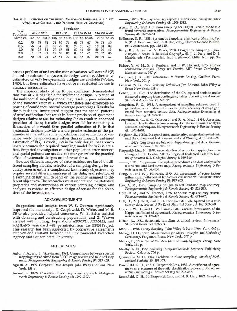
The practical consequences of applying v(ie) to a systematicdesign are effectively illustrated by examining properties of con­fidence intervals constructed with v(ie). The results for IRS arepresented first to verify that the simulation algorithm operatedcorrectly. For IRS, observed confidence interval coverage wasclose to the expected 80 percent except when sample size wassmall (Table 8). Sample sizes less than approximately 60 were

5.000

V(ie) = L (ie; - K)o/5,000,i-1

apparently too small to satisfy the asymptotic (large sample)assumption used in the derivation of v(ie), but otherwise thesimulation results for IRS were as predicted by theory.

Observed confidence interval coverage for the two systematicdesigns depended on the design effect for estimating K. Forexample, for population DIAGONAL, in which precision of thesystematic designs was worse than IRS, observed coverage ofthe confidence intervals for K from 55 and SSU5 was less thanthe nominal 80 percent. Conversely, for populations AIRPORTland MASSLAND, in which 55 and 5SUS had better precision thanIRS, observed confidence interval coverage of SS and 5SU5 washigher than the nominal 80 percent except for the 0.2 percentsamples. The confidence interval coverage properties reflectedthe general result that v(ie) underestimated V(ie) when the sys­tematic designs were less precise than IRS, and overestimatedV(ie) when the systematic designs were more precise than IRS.

CONCLUSIONS

Recommendation for use of a systematic design or SRS de­pends on the spatial pattern of misclassification and the objec­tives of accuracy assessment in a given application. If the primaryobjective is to estimate P, sampling designs should be comparedon the criterion of precision, V(P). Based on the populationsstudied, and consistent with the results reviewed in the Intro­duction, systematic designs are generally more precise, andtherefore use sampling resources more efficiently, than SRS. 55offers the greatest potential gains and losses in precision relativeto SRS. If strong periodicity in the spatial pattern of misclassi­fications is suspected, 55 and SSUS should be avoided, unlesssufficient information is available to avoid an unfavorable sam­pling interval (Matern, 1986, p. 66). It is important to recognizethat even if SUCh, an unfavorable sampling interval were se­lected, biases of P and ie are still negligible for systematic de­signs.

If a systematic design is selected, estimation of variance re­quires special consideration. The common procedure of usingV(P) to estimate the systematic design variance does not wor,kwell if the de~ign effect is not close to 1. However, because V(P)estimates V(P), of SRS even when the actual sampling design is55 or SSUS, V(P) provides a conservative estimate (Le., overes­timate) of the systematic design variance if the design effect isless than 1. In this circumstance, the precision of the systematicdesign is better than that of 5RS, but the estimate of the system­atic design variance will not reflect the improvement in preci­sion. Conversely, if the design effect is greater than 1, the more

(5)

0.97 0.970.82 0.890.57 0.890.36 0.560.42 0.57

MASSLANDSS SSUS

PopulationBLOCK DIAGONAL

SS SSUS SS SSUS0.78 1.00 1.00 1.170.88 0.97 1.18 1.431.70 0.89 3.43 1.620.86 0.57 5.86 1.461.15 0.81 2.97 1.96

AIRPORTlSS SSUS

1.03 0.950.90 0.830.43 0.730.20 0.440.21 0.39

0.20.51.03.05.0

% ofPopulationSampled

TABLE 7. ESTIMATED BIAS OF K

AIRPORTl BLOCK

Sample Sampling Design Sample Sampling DesignSize IRS SS SSUS Size IRS SS

12 -0.0186 -0.0172 -0.0207 14 -0.0209 -0.015129 -0.0068 -0.0135 -0.0078 33 -0.0092 -0.015357 -0.0034 -0.0030 -0.0050 64 -0.0030 -0.0056

226 -0.0007 -0.0003 -0.0006 256 -0.0002 0.0016352 0.0005 -0.0012 -0.0011 400 -0.0006 -0.0013

DIAGONAL MASSLAND

Sample Sampling Design Sample Sampling DesignSize IRS SS SSUS Size IRS SS

14 -0.0208 -0.0193 -0.0144 55 -0.0032 -0.001933 -0.0072 -0.0039 -0.0068 135 -0.0034 -0.001465 -0.0004 -0.0023 -0.0035 263 -0.0024 -0.0003

257 -0.0008 -0.0012 -0.0008 1051 -0.0002 -0.0007401 -0.0013 -0.0013 0.0001 1642 0.0004 -0.0003

• Sample size has been reported in this table to record the actual sample sizes represented by each sampling percentage.

SSU5-0.0233-0.0107-0.0032-0.0003-0.0016

S5US-0.0029-0.0030-0.0014-0.0001

0.0001

COMPARISON OF SAMPLING DESIGNS 1349

TABLE 8. PERCENT OF OBSERVED CONFIDENCE INTERVALS, K ± 1.28"~, THAT CONTAIN K (80 PERCENT NOMINAL COVERAGE)

Population% of

Population AIRPORT! BLOCK DIAGONAL MASSLANDSampled IRS SS SSUS IRS SS SSUS IRS SS SSUS IRS SS SSUS

0.2 75 76 74 74 80 74 69 73 67 79 78 800.5 76 84 83 78 79 80 79 73 67 79 84 821.0 76 95 84 79 67 81 80 46 69 80 90 833.0 81 92 91 79 68 85 80 16 61 79 92 865.0 80 100 94 78 81 79 80 45 57 80 94 87

serious problem of underestimation of variance will occur if v(P)is used to estim~te the systematic design variance. Alternativeestimators of V(P) for systematic designs are available (Wolter,1985), but these estimators have not been evaluated for use inaccuracy assessment.

The empirical study of the Kappa coefficient demonstratedthat bias of k is negligible for systematic designs. Violation ofthe multinomial sampling model may result in poor estimationof the standard error of k, which translates into erroneous re­porting of confidence interval coverage percentages. Results forthe populations investigated suggest that the spatial patternsof misclassification that result in better precision of systematicdesigns relative to SRS for estimating P also result in enhancedprecision of the systematic designs over IRS for estimating K.

Estimation of K would then parallel estimation of P, in thatsystematic designs provide a more precise estimate of the pa­rameter of interest for some populations, but estimation of var­iance would be approximate rather than unbiased. If unbiasedestimation of V(k) is crucial, SRS is the only design that approx­imately assures the required sampling model for v(k) is satis­fied. Empirical investigation of other population error matricesand spatial patterns are needed to better generalize the practicaleffect of systematic designs on inference for K.

Because different analyses of error matrices are based on dif­ferent sampling models, selection of a sampling design for ac­curacy assessment is a complicated task. Study objectives mayrequire several different analyses of the data, and selection ofa sampling design will depend on the priority assigned to dif­ferent objectives. The researcher must understand the statisticalproperties and assumptions of various sampling designs andanalyses to choose an effective design adequate for the objec­tives of the investigation.

ACKNOWLEDGMENTS

Suggestions and insights from W. S. Overton significantlyimproved the manuscript. R. Czaplewski, D. White, and M. B.Ritter also provided helpful comments. W. E. Bahls assistedwith obtaining and constructing populations, and G. Weaverassisted with plotting. Populations AIRPORT1, AIRPORT2, andMASSLAND were used with permission from the IDRISI Project.This research has been supported by cooperative agreementsCR815422 and CR816721 between the Environmental ProtectionAgency and Oregon State University.

REFERENCES

Agbu, P. A., and E. Nizeyimana, 1991. Comparisons between spectralmapping units derived from SPOT image texture and field soil mapunits. Photogrammetric Engineering & Remote Sensing 57: 397-405.

Agresti, A., 1989. Categorical Data Analysis. John Wiley and Sons: NewYork, 558 p.

Aronoff, S., 1982a. Classification accuracy: a user approach. Photogram­metric Engineering & Remote Sensing 48: 1299-1307.

--, 1982b. The map accuracy report: a user's view. PhotogrammetricEngineering & Remote Sensing 48: 1309-1312.

Ayeni, O. 0., 1982. Optimum sampling for Digital Terrain Models: Atrend towards automation. Photogrammetric Engineering & RemoteSensing 48: 1687-1694.

Bellhouse, D. R., 1988. Systematic Sampling. Handbook of Statistics, Vol.6, (P. R. Krishnaiah and C. R. Rao, eds.), Elsevier Science Publish­ers: Amsterdam, pp. 125-145.

Berry, B. J. L., and A. M. Baker, 1968. Geographic sampling. SpatialAnalysis: A Reader in Statistical Geography, (B. J. L. Berry and D. F.Marble, eds.) Prentice-Hall, Inc.: Englewood Cliffs, N.J., pp. 91­100.

Bishop, Y. M. M., S. E. Fienberg, and P. W. Holland, 1975. DiscreteMultivariate Analysis Theory and Practice. MIT Press: Cambridge,Massachusetts, 557 p.

Campbell, J. B., 1987. Introduction to Remote Sensing. Guilford Press:New York, 551 p.

Cochran, W. G., 1977. Sampling Techniques (3rd Edition). John Wiley &Sons: New York, 428 p.

Cohen, J. E., 1976. The distribution of the Chi-squared statistic underclustered sampling from contingency tables. Journal of the AmericanStatistical Association 71: 665-670.

Congalton, R. G., 1988. A comparison of sampling schemes used ingenerating error matrices for assessing the accuracy of maps gen­erated from remotely sensed data. Photogrammetric Engineering &Remote Sensing 54: 593-600.

Congalton, R. G., R. G. Oderwald, and R. A. Mead, 1983. AssessingLandsat classification accuracy using discrete multivariate analysisstatistical techniques. Photogrammetric Engineering & Remote Sensing49: 1671-1678.

Fingleton, B., 1983a. Independence, stationarity, categorical spatial dataand the chi-squared test. Environment and Planning A 15: 483-499.

--, 1983b. Log-linear models with dependent spatial data. Environ­ment and Planning A 15: 801-813.

Fitzpatrick-Lins, K., 1978. An.evaluation of errors in mapping land usechanges for the Central Atlantic Regional Ecological Test Site. Jour­nal of Research U.S. Geological Survey 6: 339-346.

--,1981. Comparison of sampling procedures and data analysis fora land-use and land-cover map. Photogrammetric Engineering & Re­mote Sensing 47: 343-351.

Gong, P., and P. J. Howarth, 1990. An assessment of some factorsinfluencing multispectral land-cover classification. PhotogrammetricEngineering & Remote Sensing 56: 597-603.

Hay, A. M., 1979. Sampling designs to test land-use map accuracy.Photogrammetric Engineering & Remote Sensing 45: 529-533.

Hord, R. M., and W. Brooner, 1976. Land-use map accuracy criteria.Photogrammetric Engineering & Remote Sensing 42: 671-677.

Holt, D., A. J. Scott, and P. D. Ewings, 1980. Chi-squared tests withsurvey data. Journal of the Royal Statistical Society A 143: 303-320.

Hudson, W. D., and C. W. Ramm, 1987. Correct formulation of theKappa coefficient of agreement. Photogrammetric Engineering & Re­mote Sensing 53: 421-422.

Iachan, R., 1982. Systematic sampling: A critical review. InternationalStatistical Review 50: 293-303.

Kish, L., 1965. Survey Sampling. John Wiley & Sons: New York, 643 p.Maling, D. H., 1989. Measurements for Maps: Principles and Methods of

Cartometry. Pergamon Press: New York, 577 p.Matern, B., 1986. Spatial Variation (2nd Edition). Springer-Verlag: New

York, 151 p.Murthy, M. N., 1967. Sampling Theory and Methods. Statistical Publishing

Society: Calcutta, 706 p.Quenouille, M. H., 1949. Problems in plane sampling. Annals of Math­

ematical Statistics 20: 355-375.Rosenfield, G. H., and K. Fitzpatrick-Lins, 1986. A coefficient of agree­

ment as a measure of thematic classification accuracy. Photogram­metric Engineering & Remote Sensing 52: 223-227.

Rosenfield, G. H., K. Fitzpatrick-Lins, and H. S. Ling, 1982. Sampling

1350 PHOTOGRAMMETRIC ENGINEERING & REMOTE SENSING, 1992

for thematic map accuracy testing. Photogrammetric Engineering &Remote Sensing 48: 131-137.

Rosenfield, G. H., and M. L. Melley, 1980. Applications of statistics tothematic mapping. Photogrammetric Engineering & Remote Sensing 46:1287-1294.

Skinner, C. J., D. Holt, and T. M. F. Smith, 1989. Analysis of ComplexSurveys. John Wiley & Sons: New York, 309 p.

Stenback, J. M., and R. G. Congalton, 1990. Using thematic mapperimagery to examine forest understory. Photogrammetric Engineering& Remote Sensing 56: 1285-1290.

Story, M., and R. G. Congalton, 1986. Accuracy assessment: a user'sperspective. Photogrammetric Engineering & Remote Sensing 52: 397­399.

Stuart, A., 1984. The Ideas of Sampling (3rd edition). Oxford UniversityPress: New York, 91 p.

Upton, G. J. G., and B. Fingleton, 1989. Spatial Data Analysis by Example:Volume 2. John Wiley & Sons: New York, 416 p.

Van Genderen, J. L., B. F. Lock, and P. A. Vass, 1978. Remote sensing:statistical testing of thematic map accuracy. Remote Sensing of En­vironment 7: 3-14.

Wolter, K., 1985. Introduction to Variance Estimation. Springer-Verlag:New York, 427 p.

Yates, F., 1948. Systematic sampling. Philosophical Transactions of the RoyalSociety A 241: 345-377.

(Received 26 September 1990; revised and accepted 22 January 1992)

SOFTWARE REVIEW

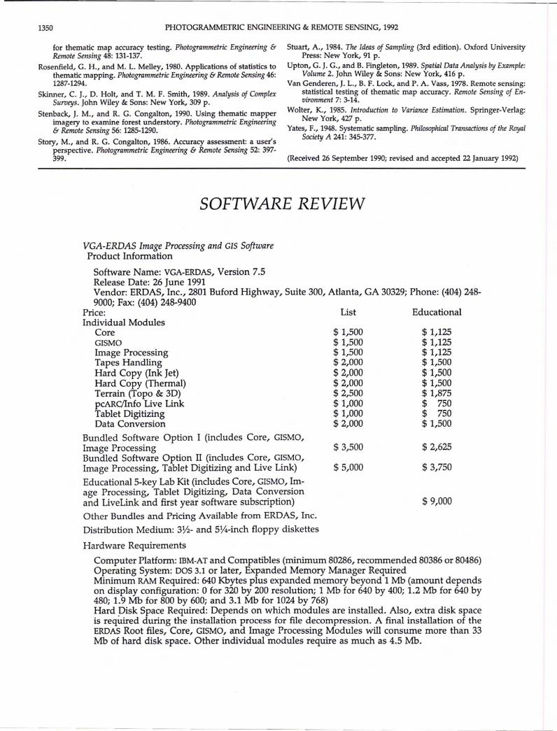
VGA-ERDAS Image Processing and GIS SoftwareProduct Information

$ 1,125$ 1,125$ 1,125$ 1,500$ 1,500$ 1,500$ 1,875$ 750$ 750$ 1,500

EducationalList

$ 1,500$ 1,500$ 1,500$ 2,000$ 2,000$ 2,000$ 2,500$ 1,000$ 1,000$ 2,000

Software Name: VGA-ERDAS, Version 7.5Release Date: 26 June 1991Vendor: ERDAS, Inc., 2801 Buford Highway, Suite 300, Atlanta, GA 30329; Phone: (404) 248­9000; Fax: (404) 248-9400

Price:Individual Modules

CoreGISMOImage ProcessingTapes HandlingHard Copy (Ink Jet)Hard Copy (Thermal)Terrain (Topo & 3D)pcARC/Info Live LinkTablet DigitizingData Conversion

Bundled Software Option I (includes Core, GISMO,Image Processing $ 3,500 $ 2,625Bundled Software Option II (includes Core, GISMO,Image Processing, Tablet Digitizing and Live Link) $ 5,000 $ 3,750

Educational5-key Lab Kit (includes Core, GISMO, Im-age Processing, Tablet Digitizing, Data Conversionand LiveLink and first year software subscription) $ 9,000

Other Bundles and Pricing Available from ERDAS, Inc.

Distribution Medium: 3'i2- and 5Yt-inch floppy diskettes

Hardware Requirements

Computer Platform: IDM-AT and Compatibles (minimum 80286, recommended 80386 or 80486)Operating System: DOS 3.1 or later, Expanded Memory Manager RequiredMinimum RAM Required: 640 Kbytes plus expanded memory beyond 1 Mb (amount dependson display configuration: 0 for 320 by 200 resolution; 1 Mb for 640 by 400; 1.2 Mb for 640 by480; 1.9 Mb for 800 by 600; and 3.1 Mb for 1024 by 768)Hard Pisk Space Required: Depends on which modules are installed. Also, extra disk spaceis required during the installation process for file decompression. A final installation of theERDAS Root files, Core, GISMO, and Image Processing Modules will consume more than 33Mb of hard disk space. Other individual modules require as much as 4.5 Mb.