International Conference on Urban and Regional Planning 2014

Comparison of Spatial Autocorrelation Analysis Methods for Distribution Pattern of Diabetes Type II Patients in Iskandar Malaysia Neighbourhoods

M. AIZAT SAIFUL BAHRI1, SOHEIL SABRI1, FOZIAH JOHAR1, ZOHREH

KARBASSI2, M. RAFEE MAJID1, AHMAD NAZRI MUHAMAD LUDIN1 1 Center for Innovative Planning and Development (CiPD), Faculty of Built Environment, Universiti Teknologi

Malaysia 2 Jeffery Cheh School of Medicine and Health Sciences, Clinical School, Johor Bahru, Monash University

Malaysia, Email address: 1 mohdaizatsaifulbahri@gmail.com

ABSTRACT Spatial statistics have been widely used in epidemiology studies in order to investigate and monitor the outbreak in endemic area. However, there is less application of spatial statistics in the study on built environment and diseases outbreak. It is significant to conduct such a study since non-communicable diseases have been rising over past four decades and have a strong positive relation to the built environment, particularly in the rapid urbanizing area. Therefore, this study aims to measure the geographical distribution and determine the pattern of the patients in urbanizing area. Two methods of Moran’s I and Getis-Ord G Statistics, that have been used extensively in the epidemiology are compared on diabetes type II patients data both in global and local scales. A total of 496 patients diagnosed with diabetes type II in 154 neighbourhoods of Iskandar Malaysia (IM) have been evaluated. This study compares the results of two methods based on built environment criteria. The study evaluates their applicability is such a study to identify the best method and scale to be considered in study on built environment-related epidemiology. KEYWORDS Spatial Autocorrelation, Diabetes Type II, Iskandar Malaysia, Built Environment-related epidemiology

Page 1

International Conference on Urban and Regional Planning 2014 1. INTRODUCTION

Epidemiology has been defined as the study of the distribution and factor of health-related events in specified population to control and monitor health problem. It provides information on risk factors for disease, thus steps and action can be taken to prevent disease incidence (Last, 2001; Ward, 2008). As the development of spatial statistical methods has driven the spatial epidemiology to develop as a sub-discipline since most studies currently apply epidemiologic principles and analytical methods to understand disease occurrence (Elliot & Wartenberg, 2004).

In general, spatial analysis or spatial statistics is the Geographical Information System

(GIS) operation which clearly involves geographical data either in the form of point, line or polygon. Spatial analysis of geographical data may answer the questions as mention by Camara et al (2011) which are: (i) do the distribution of cases of a disease form a pattern in space? (ii) Is there is any spatial concentration in the distribution? (iii) Is there is underlying factors causes the outbreak? Until now, GIS and spatial analysis were frequently used to portray the pattern of the diseases. For instance, in Malaysia, purely spatial and retrospective analysis was used to determine the clustering and distribution pattern of the Dengue incidence in Gombak district (Doss et al, 2013). In China, spatial and retrospective space-time scan statistics analysis was used to describe the distribution pattern of Tuberculosis in Linyi city (Wang et al, 2012). In Canada, an exploratory spatial analysis was conducted in order to determine the overweight and obesity (Poulio & Elliot, 2009). In Spain, spatial analysis and ecological was used to determine the hot spot and cold spot of depression as a risk factor to the severe health problem (Perez et. al, 2012). This indicate that a better understanding of the spatial epidemiology may assist the public health sector to provide guideline for formulating prevention and control strategies as the best remedy is the prevention (Maciel et. al, 2010; Wang et. al, 2012).

However, far too little attention has been given to the application of spatial statistics

in the study on built environment and diseases outbreak. Recent developments in public health studies (Block, Scribner & DeSalvo, 2004; Lee & Vernez, 2008; Bhzad & Mohamed, 2012) have highlighted a strong association between health behaviour and built environment. Factors of built environment are beyond the socio-economic, and neighbourhood deprivation, which have been studied in many epidemiological researches (White et al., 2011; Reiss, 2013). Increasing rate of many non-communicable diseases, such as cardiovascular disease, diabetes, and obesity, are directly associated with the level of urbanization, and lack of physical activity (Daar et al., 2007; Bai et al., 2012). This paper examines the significance of applying spatial analysis of a non-communicable disease in a rapid urbanizing area. The study compares two common spatial autocorrelation analysis methods for examining the geographical distribution pattern of patients with diabetes mellitus type 2 in IM. The paper focuses on an exploratory analysis of spatial patterns using two methods of Moran’s I and Getis-Ord G statistics and compares their results using built-environment factors. The paper ultimately intends to identify the suitable methods and scale to be considered in study on built environment-related epidemiology. The next section of this paper gives a brief overview of spatial autocorrelation and its application in health studies to set a conceptual framework. In the fourth section, the results of analyses are presented and evaluated using built-environment factors. Finally, the discussion and conclusion section summaries the findings and addresses their implications to future research on public health and built-environment area.

Page 2

International Conference on Urban and Regional Planning 2014 2. CONCEPTUAL FRAMEWORK

Spatial autocorrelation can be described as based on Tobler’s first law of geography, which is “everything is related to everything else, but near things are more related than distant things”. In other word, spatial autocorrelation can be interpreted as the extent to the value of variable at one location (area) is related to the values of the variable nearby in locations (areas) (Malczewski, 2010).

As the growing body of literature on analysis of spatial association for epidemiology

study, there is questions arise for which suitable spatial statistics can be considered particularly in the interdisciplinary study such built environment-related epidemiology (Li, Kim, & Farley, 2010). As in the context of spatial autocorrelation in health, many studies (Poulio & Elliot, 2009; Schuurman et al., 2009) which measuring the spatial association of obesity, have focused on the national or provincial level of spatial associations where there is less studies that focusing on the neighbourhood level.

This study however, in the context of rapid urbanizing area is focusing in on the neighbourhood level and considered the patient density in the each neighbourhood as the variable while the spatial units is based on the neighbourhood boundaries in IM. The consideration of the neighbourhood as the spatial units was motivated by the availability of relevant datasets. The density of the patient in each neighbourhood in IM was calculated using the formula of number of patient (each neighbourhood) divided by the area of the neighbourhood boundaries. The analysis of the spatial patterns of diabetes mellitus type 2 was focusing on the local scales of spatial statistics as the local measures examines specific neighbourhood in order to determine the clustering of high (hot spot) and low (cold spot) value. Figure 1 shows the conceptual framework for this study.

Figure 1: Conceptual framework

Page 3

International Conference on Urban and Regional Planning 2014 3. MATERIAL AND METHODS

3.1 Study Area

The study area involved in this research is located at the southern-most tip of peninsular Malaysia and mainland Asia which is Iskandar Malaysia (IM) that regulated by Iskandar Region Development Authority (IRDA). IM consists of five local authorities which are Kulai District Council (MPK), Pontian District Council (MDP), Central Johor Bahru Municipalities (MPJBT), Johor Bahru City Council (MBJB) and Pasir Gudang Municipalities (MPPG). IM region has been identified as one of the catalysts for GDP growth in the nation by the 10th Malaysia Plan through high-impact developments, with an investment of RM 43 billion. Due to this initiation, the city-region has experienced low density sprawl into pre-existing rural land covering an area of over 2217 square km (Nasongkhla & Sintusingha, 2012). IM have been experiencing land use changes from 2006 – 2011 where the agriculture to built-up area land use changes from 90.97% to 61.01% covering 20748.29 hectares in 2011 compared to 2006 which 15109.12 hectares. Thus, it is essential for this rapid development to establish a framework that takes into consideration a high public health standard since its aims to developed IM as the main corridor for future economic development (KN, 2006). Figure 2 shows the study area. 3.2 Data Collection and Source

The target group of active type 2 diabetes has been identified. Through the questionnaire conducted by medical experts in three different clinics located in Iskandar Malaysia region namely Mahmoodiah Clinic, Tampoi Clinic and Kempas Clinic, all the respondents social and demographics data were obtained. The social information of diabetes patient was extracted from the questionnaire. The survey was conducted on 503 patients. The data is categorised according to socio-demographic (i.e. age, gender, marital status, occupation, etc.); lifestyle (i.e. physical activity type and duration per day/week, smoking, alcohol, family history, etc.); and physiological (i.e. Body Mass Index (BMI), Vascular System, Blood Pressure, Cholesterol level, etc.) The questionnaire was conducted in early 2013. As a result 496 records have been decided to be considered in analysis. A geodatabase was developed based on the patient information and their locations were geocoded using Esri ArcGIS 10. All incomplete data were excluded in order to avoid any biasness in the analysis. The built-environment data were obtained from Iskandar Regional Development Authorities (IRDA). Data that were obtained from IRDA was in the digital form which comprised of road network, land use and boundaries of neighbourhood in Iskandar Malaysia. The boundaries data were updated using digitizing and visual comparison methods and updated by patient density attributes. A total of 155 out of 438 neighbourhoods were considered to be included in this study.

Page 4

International Conference on Urban and Regional Planning 2014

Figure 2: Study Area

Page 5

International Conference on Urban and Regional Planning 2014 3.3 Analysing Patterns (Global Spatial Autocorrelation)

To investigate the general spatial distribution patterns of patients, two spatial autocorrelation methods have been used in this study namely Moran’s I spatial autocorrelation, and the general G(d) statistic. The Moran’s I statistic is the product-moment coefficient (Getis, 2010) and it measures spatial autocorrelation based on both feature locations and feature values. The numerator of the coefficient is a cross-products covariance term and the denominator contains a variance term (Malczewski, 2010). If areas in a certain distances have a similar density of diabetes patient, then the value is either two positive or two negative (positive autocorrelation) while if the areas in a certain distances is dissimilar of density it will exhibits negative autocorrelation. Moran’s I values usually fall between -1.0 and +1.0 for maximum positive and negative. Moran’s I can be express as,

𝐼𝐼 =𝑛𝑛∑ ∑ 𝑤𝑤𝑖𝑖, 𝑧𝑧𝑖𝑖𝑧𝑧𝑗𝑗𝑛𝑛

𝑗𝑗=1𝑛𝑛𝑖𝑖=1

𝑆𝑆𝑆𝑆 ∑ 𝑧𝑧𝑖𝑖2𝑛𝑛𝑖𝑖=1

The expected value of Moran’s I can be express as𝐸𝐸(𝐼𝐼) = −1/(𝑛𝑛 − 1) , where 𝐸𝐸(𝐼𝐼) = Expected Index value, while I = Observed Index value and n = 154 (number of neighbourhood). Value of I that is more than E(I) indicate positive spatial autocorrelation which is similar value is spatially clustered. Value of I that is less than E(I) indicate negative spatial autocorrelation which is dissimilar value in neighbouring. However, the Moran’s I statistic cannot distinguish if the similarity of the values is due to high values or low values, in other word, the different between two types of spatial autocorrelation (Wong & Lee, 2005, Malczewski, 2010). The general G(d) statistics (Getis & Ord, 1992) can avoid the limitation of differentiate two type of spatial autocorrelation. The statistic is based on cross-product statistics and can be defined as the ratio of cross-product values within certain distance to the sum of all values in study area (Getis, 2010). The general G(d) statistic can be defined as 𝐸𝐸(𝐺𝐺) = 𝑊𝑊/[𝑛𝑛(𝑛𝑛 − 1)] where, 𝑊𝑊 = ∑∑𝑊𝑊𝑖𝑖𝑗𝑗(𝑑𝑑), and n = the number of neighbourhoods. A positive z-score value indicates relatively spatial clustering of high values for attributes in study area, whereas a negative z-score value indicates relatively spatial clustering of low values for attributes. 3.4 Mapping Clusters (Local Spatial Autocorrelation)

The local measure of spatial statistic measures the dependence of the value of a variable at any one area upon neighbouring values of that variable (Malczewski, 2010). In other words, the local measure of spatial statistic is concentrated and focused on the neighbouring value a in particular study area. Two types of local spatial statistics were in this study, namely, the local Moran’s I and the local Gi* statistic. Similar to the global measure of Moran’s I, the local Moran’s I measures the spatial clusters of features with similar value in neighbouring target area. A positive value of I indicates that the features being evaluate has a neighbouring features that are similar value either high or low. In addition, the statistical significance level of local Moran’s I was express through the z-score and p-value.

Page 6

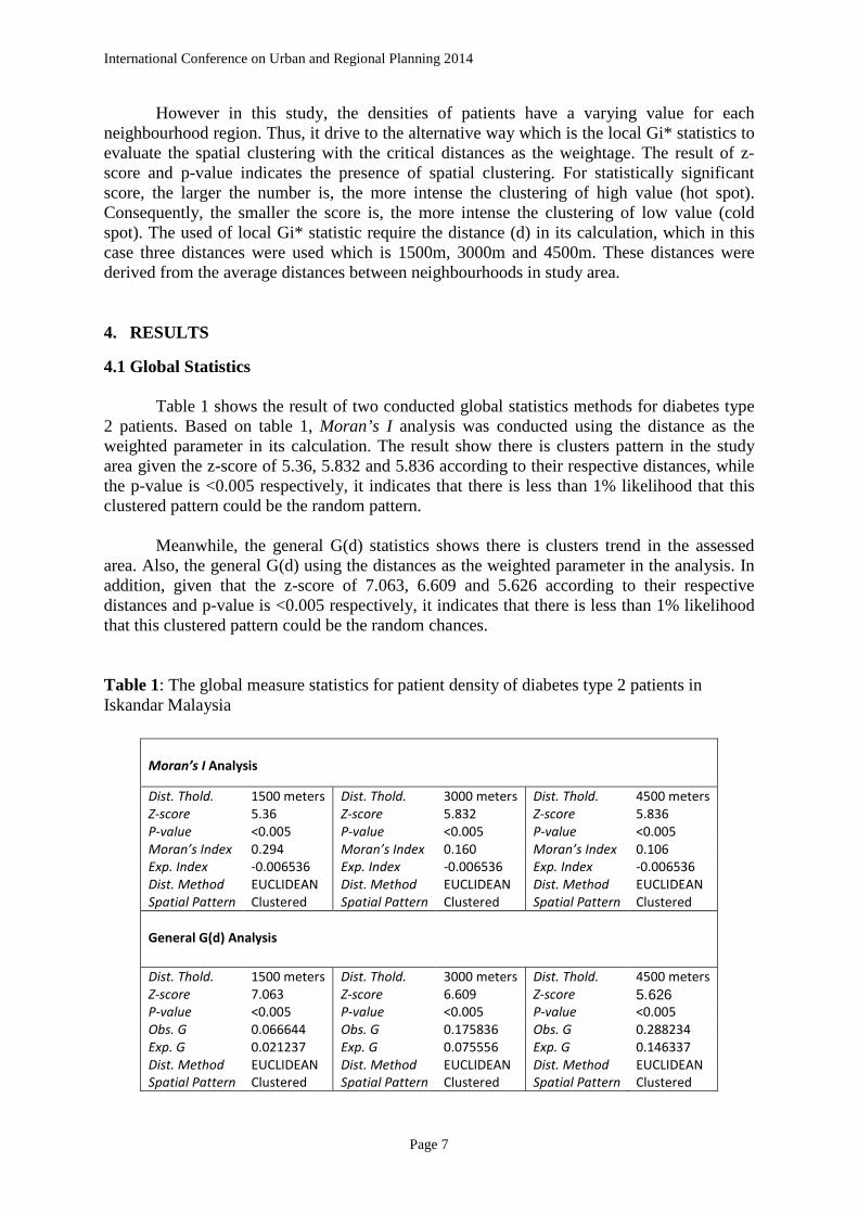
International Conference on Urban and Regional Planning 2014 However in this study, the densities of patients have a varying value for each neighbourhood region. Thus, it drive to the alternative way which is the local Gi* statistics to evaluate the spatial clustering with the critical distances as the weightage. The result of z-score and p-value indicates the presence of spatial clustering. For statistically significant score, the larger the number is, the more intense the clustering of high value (hot spot). Consequently, the smaller the score is, the more intense the clustering of low value (cold spot). The used of local Gi* statistic require the distance (d) in its calculation, which in this case three distances were used which is 1500m, 3000m and 4500m. These distances were derived from the average distances between neighbourhoods in study area. 4. RESULTS

4.1 Global Statistics Table 1 shows the result of two conducted global statistics methods for diabetes type 2 patients. Based on table 1, Moran’s I analysis was conducted using the distance as the weighted parameter in its calculation. The result show there is clusters pattern in the study area given the z-score of 5.36, 5.832 and 5.836 according to their respective distances, while the p-value is <0.005 respectively, it indicates that there is less than 1% likelihood that this clustered pattern could be the random pattern.

Meanwhile, the general G(d) statistics shows there is clusters trend in the assessed

area. Also, the general G(d) using the distances as the weighted parameter in the analysis. In addition, given that the z-score of 7.063, 6.609 and 5.626 according to their respective distances and p-value is <0.005 respectively, it indicates that there is less than 1% likelihood that this clustered pattern could be the random chances. Table 1: The global measure statistics for patient density of diabetes type 2 patients in Iskandar Malaysia

Moran’s I Analysis

Dist. Thold. 1500 meters Dist. Thold. 3000 meters Dist. Thold. 4500 meters Z-score 5.36 Z-score 5.832 Z-score 5.836 P-value <0.005 P-value <0.005 P-value <0.005 Moran’s Index 0.294 Moran’s Index 0.160 Moran’s Index 0.106 Exp. Index -0.006536 Exp. Index -0.006536 Exp. Index -0.006536 Dist. Method EUCLIDEAN Dist. Method EUCLIDEAN Dist. Method EUCLIDEAN Spatial Pattern Clustered Spatial Pattern Clustered Spatial Pattern Clustered

General G(d) Analysis

Dist. Thold. 1500 meters Dist. Thold. 3000 meters Dist. Thold. 4500 meters Z-score 7.063 Z-score 6.609 Z-score 5.626 P-value <0.005 P-value <0.005 P-value <0.005 Obs. G 0.066644 Obs. G 0.175836 Obs. G 0.288234 Exp. G 0.021237 Exp. G 0.075556 Exp. G 0.146337 Dist. Method EUCLIDEAN Dist. Method EUCLIDEAN Dist. Method EUCLIDEAN Spatial Pattern Clustered Spatial Pattern Clustered Spatial Pattern Clustered

Page 7

International Conference on Urban and Regional Planning 2014 4.2 Local Statistics Figure 2 shows the result of spatial clusters of the patient density of diabetes type 2 patients. The local Moran’s I statistic indicates the extent of significant spatial clusters in the assessed neighbourhood are clustering of the similar value of attributes. The value are classified into four categories which are (i) neighbourhood with high density of patient surrounded by high density of patient (H-H), (ii) neighbourhood with low density of patient surrounded by low density of patient (L-L), (iii) neighbourhood with high density surrounded by low density of patient (H-L), and (iv) neighbourhood with low density surrounded by high density of patient (L-H). The local Moran’s I statistics has been conducted with the weighted parameter of distance which is 1500m, 3000m and 4500m, which is the considerable average of distance between neighbourhood. It reveals that the presence of neighbourhood clusters is mostly located in the central parts of the study area which indicates the high density of diabetes patient (figure 7a, b, and c). However, there is outlier existence in the weight parameter of 1500m distance (figure 7b) which indicates the unexpected value of dissimilar value with p-value of <0.005. a)

b)

Figure 3: Local Moran’s I statistic maps: diabetes type 2 patient

density

(a) 1500m (b) 3000m (c) 4500m

Page 8

International Conference on Urban and Regional Planning 2014 c)

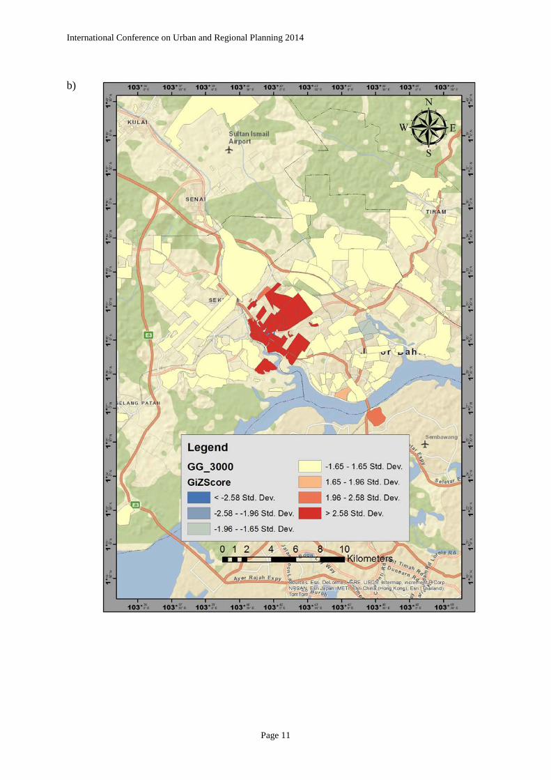
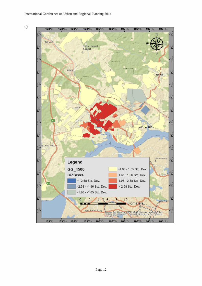
In the same way, the local G* statistic was carried out in the same weight distance parameter as the local Moran’s I which are three distance band of 1500m, 3000m and 4500m. The result reveals that there is a statistically significant spatial cluster in the three distance bands. Given that the z-score >2.58 Std. Dev., the clustering of the neighbourhood with highest density tend to be located in central part of the study area. The local G* statistic indicate that the larger of positive z-score is the intense the clustering of high value (hot spot) similarly, the larger the z-score towards negative, the intense the clustering of low value (cold spot). In this case however, while there is significantly spatial clustering in three distances, there are two cold spot presences in the study area which located at the east of central parts (figure c). Figure 3a, b and c shows the result of the local G* statistic in the study area.

Page 9

International Conference on Urban and Regional Planning 2014 a)

Figure 4: The local Gi* significance map of patient density (a) 1500m (b) 3000m (c) 4500m

Page 10

International Conference on Urban and Regional Planning 2014 b)

Page 11

International Conference on Urban and Regional Planning 2014 c)

Page 12

International Conference on Urban and Regional Planning 2014 Table 2 and 3 below shows the comparison table of the result in respect of the built environment features in the statistically significant clusters of the neighbourhood in the study area base on the average distance between neighbourhood which is 3000m.

Table 2: Moran’s I Result

Neighbourhood Name

Housing types Recreation (%)

Commercial (%)

Z score

P value

Type Condo/ Flat

Terrace/ Detach

Taman Cempaka 26 2196 0 0.94 6.490 0 HH Taman Dahlia 8 1328 1.99 1.24 6.490 0 HH Taman Dato Penggawa Barat

- 665 1.9 5.93 2.162 0.030 HH

Taman Impian Skudai

- 321 0 0 4.922 0 HH

Taman Kemas - 855 1.9 4.57 6.490 0 HH Taman Kobena - 519 4.01 3.93 3.614 0.0001 HH Taman Melor - 1551 8.4 0 11.728 0 HH Taman Orkid - 118 6.92 0.89 3.889 0.0001 HH Taman Skudai Kanan 1 1083 0.4 5.41 5.232 0 HH Taman Sri Bahagia - 444 0.88 8.45 2.159 0.0307 HH Taman Tampoi Indah II

- 3816 4.5 0 2.157 0.0309 HH

Bandar Baru Uda - 4736 2.49 2.36 5.232 0 HH Taman Kim Teng 4 - 0 0 -6.554 0 LH Taman Desa Rahmat - 431 3.24 3.71 10.908 0 HH Taman Melati 4 - 0 0 2.140 0.032 HH Kempas Banjaran - 621 0.19 0.23 -2.141 0.032 LH

Page 13

International Conference on Urban and Regional Planning 2014

Table 3: Gi* Statistic

Neighbourhood Name

Housing types Recreation (%)

Commercial (%)

Z score

P value Condo/

Flat Terrace/ Detach

Bandar Baru Uda - 4736 2.49 2.36 2.795 0.005 Taman Tampoi Indah II - 3816 4.50 0 4.002 0.000 Taman Tampoi Indah - 3035 4.60 45.49 3.823 0.000 Taman Tampoi Utama - 2363 6.76 8.33 4.024 0.000 Taman Cempaka 26 2196 0 0.94 4.003 0.000 Taman Bukit Mewah - 2073 1.15 2.05 2.510 0.012 Taman Bukit Kempas - 1969 2.43 2.36 4.024 0.000 Taman Dahlia 8 1328 1.99 1.24 3.602 0.000 Taman Melor - 1151 8.4 0 2.510 0.012 Taman Anggerik - 1117 4.38 3.7 2.795 0.005 Taman Skudai Kanan 1 1083 0.4 5.41 2.927 0.003 Taman Sutera Utama - 1030 3.91 3.98 4.024 0.000 Taman Johor - 913 3.72 1.17 4.024 0.000 Taman Kemas - 855 1.9 4.57 4.003 0.000 Taman Dato Penggawa Barat - 665 1.9 5.93 3.622 0.000 Taman Kobena - 519 4.01 3.93 2.945 0.003 Taman Sri Bahagia - 444 0.88 8.45 3.622 0.000 Taman Tampoi - 385 0.15 23.19 2.340 0.019 Taman Impian Skudai - 321 0 0 2.510 0.012

Taman Sri Putra - 310 0 0.125 -

1.707 0.088

Stulang Bahru - 121 7.74 0 4.024 0.000 Taman Orkid - 118 0 0.94 4.003 0.000 Taman Desa Rahmat - 431 3.24 3.71 3.993 0.000 Taman Melati 4 - 0 0 3.959 0.000 Taman Kenanga 13 - 1.34 0 4.024 0.000 Kempas Baru - 647 2.83 0.41 4.024 0.000 Kampung Sri Kempas - 214 2.49 1.84 4.024 0.000 Kempas Banjaran - 478 0.19 0.23 4.017 0.000 Kampung Seri Serdang - 128 0.55 0.32 2.631 0.009 Kampung Pasir - 446 0.82 2.53 3.622 0.000 Kampung Pengkalan Rinting - 9 0 0.92 3.381 0.001 Kampung Skudai Kiri - 292 0.16 8.34 4.284 0.000 Kuarters HSA - 109 0.71 0.56 3.430 0.001 Kampung Setanggi - 150 0.64 0 1.669 0.095 Kampung Dato Sulaiman Menteri

- 521 2.07 1.27 -1.700

0.089

Kampung Bendahara - 355 1.23 0.44 -1.700

0.089

Kampung Sinaran Baru - 11 0 0 -1.854

0.064

Woodland Straits - - 0 0 2.634 0.008

Page 14

International Conference on Urban and Regional Planning 2014 5. DISCUSSION AND CONCLUSION

The objective of this study was to compare two methods of spatial autocorrelation and evaluate their accuracy in order to identify the best method and scale to be considered in a study on built environment-related epidemiology. To do so, we conducted the spatial autocorrelation analysis namely Moran’s I and Getis Ord statistics both global and local measure on the density of the diabetes type 2 patients. First, the global measure of Moran’s I statistics was used to determine the significance of spatial clustering based on the similar attributes value of high or low. Second, the global general G (d) statistic was used to determine the degree of significance spatial clustering based on the high or low value of attributes. Thus, we looked to the processes behind the spatial autocorrelation and spatial pattern as a mechanism to comparing the suitable method for this study.

Complementary to this, based on table 4, the global measure of the spatial autocorrelation

of two methods reveals a relatively significant spatial clustering, indicates that spatial clustering of density of diabetes type 2 patient presences. The local Moran’s I includes the similar value of attributes either high or low in the given area. Conversely, the global Moran’s I statistic cannot distinguish if the similarity of the values is due to high values or low values in other words, the indices of Moran’s I are concern with only whether neighbouring values are similar or not (Wong & Lee, 2005). Thus, this has led the study to conduct the general G(d) statistic that will avoid this limitation where, the general G(d) statistic include the critical distance (d) in its equation. Unlike the global Moran’s I, the feature of high value in general G(d) statistics need to be surrounded by high values as well in order to be statistically significant (Esri, 2013).

Subsequently, the local measure of spatial autocorrelation was conducted to measure the suitability of the methods in built environment related epidemiology. Like the global measure of Moran’s I, the local measure of Moran’s I also measure the degree of variable value (attributes) in target area is similar to the values (attribute) of that variables in by neighbourhood area (Anselin, 1995; Malczewski, 2010). Similar to the global measure of general G(d) statistics, the local version of Gi* statistics includes the critical distance of target value in its calculation and because of the inclusion of the target value it makes the statistics more appropriate for this study. It should be emphasized that this comparison of spatial autocorrelation analysis should not be a standard measurement of built environment related epidemiology study. Perhaps this study would give a view on suitable methods for this kind of study. This argument is, at least supported by the spatial autocorrelation analysis. Although, the spatial clusters pattern of diabetes type 2 may suggest the underlying factors of its clustering. This type of analysis can lead to the important discoveries over the pattern occurred and required a further and direct studies.

Page 15

International Conference on Urban and Regional Planning 2014

Table 4: Comparing methods for spatial autocorrelation

Method Statistic Scale of measurement

Significance test

Advantages Disadvantages

Global Moran’s

I

Product-moment

correlation coefficient

Global z-score and p-value

Measuring the concentration of similar values of study area either high or low

- Does not distinguish the dissimilar value closeness.

General

G Statistic

Cross-product

Global z-score and p-value

Measure the concentration of high and low values and considering the (d) distance

- Need to consider the weightage critical distance (d) in its calculation

Local Moran’s

I

Product-moment

correlation coefficient

Local z-score and p-value

Concentration of similar values in study area and spatial outlier

- Does not distinguish the dissimilar value closeness.

G*(d)

statistic Cross-

product Local z-score and

p-value Identifies spatial clusters of high values (hot spots) and low values (cold spots)

- Does not have spatial outlier

6. ACKNOWLEDGEMENT

We would like to thank to the Universiti Teknologi Malaysia for the Research University Grant (06J92) for funding to this study.

Page 16

International Conference on Urban and Regional Planning 2014 7. REFERENCES

Aldstadt J., (2010). Handbook of Applied Spatial Analysis: Software Tools, Methods and Applications, M.M. Fischer and A. Getis (eds.), DOI 10.1007/978-3-642-03647-7_15, (279-300)

Anselin, L. (1995). Local indicators of spatial association - LISA. Geographical Analysis, 27, 93–115.

Bai, X.M., I. Nath, T. Capon, N. Hasan, D. Jaron., (2012). Health and wellbeing in the

changing urban environment: Complex challenges, scientific responses, and the way forward. Current Opinion on Environmental Sustainability 4: 465-472.

Bhzad Sidawi & Mohamed Taha Ali Al-Hariri, (2012). The Impact of Built Environment on

Diabetic Patients: The Case of Eastern Province, Kingdom of Saudi Arabia.

Block J., P., Scribner R., A., & DeSalvo K., B., (2004). Fast Food, Race/Ethnicity, And Income A Geographic Analysis. Am J Prev Med 2004; 27 (3):211–217).

Camara, G., Monteiro, A., M., Fucks, S., D., & Carvalho, M., S., (2011). Spatial Analysis and GIS: A Primer. Image Processing Division, National Institute for Space Research (INPE), Brazilian Agricultural Research Agency (EMBRAPA).

Doss J., I., Chinna K., Aziz Shafie, Sabrina Che Soh, (2013). Geo-Statistical Modeling Analysis of Dengue Incidence in Gombak District Malaysia. Health GIS. Proceeding of

5th International Conference. Pg. 214.

Elliot P., and Wartenberg D., (2004). Spatial Epidemiology: Current Approaches and Future Challenges. Mini-Monograph Environmental Health Perspectives Vol. 112 No. 9. Esri. (2013). Arcgis Desktop Help: How Hot Spot Analysis (Getis-Ord Gi*) Works.

http://help.arcgis.com/en/arcgisdesktop/10.0/help/index.html#//005p00000011000000 (accessed on 5th April 2014)

Getis A., (2010). Handbook of Applied Spatial Analysis: Software Tools, Methods and Applications, M.M. Fischer and A. Getis (eds.), DOI 10.1007/978-3-642-03647-7_15, (255-278)

Getis A., and J., K., Ord. (1992). The Analysis of Spatial Association by Use of Distance Statistics. Geographical Analysis 24: 189-206. KN (Khazanah Nasional), (2006). Comprehensive Development Plan for South Johor

Economic Region 2006–2025. KL. November.

Last, J.M. (2001). A dictionary of epidemiology (4th ed.). (Oxford: Oxford University Press) (accessed on 9th April 2014) Lee, C., Vernez M., A., (2008). Neighbourhood design and physical activity. Building

Research & Information ISSN 0961-3218 print ⁄ISSN 1466-4321 online.

Page 17

International Conference on Urban and Regional Planning 2014

Li A., A. Kim., E. Farley, (2010). Diabetes and the built environment: Contributions from an

emerging interdisciplinary research program. Diabetes and the built environment. University Of Western Ontario Medical Journal 79:1 pg 20.

Maciel EL, Pan W, Dietze R, Peres RL, Vinhas SA, Ribeiro FK, Palaci M, Rodrigues RR, Zandonade E, Golub JE (2010). Spatial patterns of pulmonary tuberculosis incidence and their relationship to socio economic status in Vitoria, Brazil. Int J Tuberc Lung Dis 2010, 14(11):1395–1402.

Malczewski J., (2010). Exploring spatial autocorrelation of life expectancy in Poland with global and local statistics. GeoJournal (2010) 75:79–92 DOI 10.1007/s10708-009-9278-5

Moran PAP (1950) Notes on continuous stochastic phenomena. Biometrika 37(12):17-23.

Nasongkhla, S., & Sintusingha, S. (2012). Social Production of Space in Johor Bahru. Urban Studies, 0042098012465907–. doi:10.1177/0042098012465907

Perez J., A., S., Alonso C., R., G., Parilla C., M., Sampietro E., J., Carulla L., S., (2012). Identification and location of hot and cold spots of treated prevalence of depression in Catalonia (Spain). Int. J Health Geogr. 2012; 11: 36.

Poulio T., and Elliot S., J., (2009). An exploratory spatial analysis of overweight and obesity in Canada. Preventive Medicine 48 (2009) 362–367. 2009 Elsevier Inc. Scott L., M., and Janikas M., (2010). Handbook of Applied Spatial Analysis: Software Tools,

Methods and Applications, M.M. Fischer and A. Getis (eds.), DOI 10.1007/978-3-642-03647-7_15, (255-278)

Wang T., Xue F., Chen Y., Ma Y. and Liu Y., (2012). The spatial epidemiology of tuberculosis in Linyi City, China, 2005–2010. BMC Public Health 2012, 12:885. Ward. M., (2008). Geospatial Technologies and Homeland Security. Research Frontiers and

Future Challenges. The GeoJurnal Library Vol. 94. Springer Science + Business Media B.V. 2008.

White H, Matheson F, Moineddin R, Dunn J, Glazier R., (2011). Neighbourhood deprivation and regional inequalities in self-reported health among Canadians: are we equally at risk?. Health Place 2011;17:361-9 Wong D., W., S., & Lee J., (2005). Statistical Analysis of Geographic Information with ArcView and ArcGIS. Pg 367 Pp 1-2. John Wiley & Sons Inc.

Page 18