Embed Size (px)
Citation preview

Comparison of several solution methods forthe Euler equations in a finite volume code
Tamil Iniyan ManokaranMatrikelnummer 4744573
Examiner: Prof. Dr.-Ing. habil. Cord-Christian RossowDeutsches Zentrum fur Luft- und Raumfahrt (DLR)Institut fur Aerodynamik und Stromungstechnik
Supervisor: Dr. habil. Stefan LangerDeutsches Zentrum fur Luft- und Raumfahrt (DLR)Institut fur Aerodynamik und Stromungstechnik
Submission date: 20 September 2018


1
DeclerationI, Tamil Iniyan Manokaran born on 27.05.1994 hereby declare that the projectwork entitled Comparison of several solution methods for the Euler equations in afinite volume code submitted to the Deutsches Zentrum fur Luft- und Raumfahrt(DLR), Braunschweig is a record of an original work done by me under the guid-ance of Dr. habil. Stefan Langer, Deutsches Zentrum fur Luft- und Raumfahrt(DLR), Braunschweig and this project work is submitted in the partial fulfillmentof the requirements for the award of the degree of Master of Computational Sci-ences in Engineering. The results embodied in this thesis have not been submittedto any other University or Institute for the award of any other degree.
Braunschweig, 20.09.2018


2
AbstractI would like to start the thesis with an Einstein’s quote, which admired most”Make things as simple as possible, but not simpler”.
One of the most popular and simple methods to derive a non-linear equation tosteady state is diagonal implicit Runge-Kutta method. This method leads us to geta final linear equation. Then we would like to solve that linear equation with anyof the iterative solvers to get efficiently an approximate solution.
These solution methods can be often used as smoother in a nonlinear multigridalgorithm. The actual solution depends on the approximation of the derivative ofthe nonlinear equation and on the iterative method to approximately solve the lin-ear equation.
Goal of the Studienarbeit is the implementation of a two dimensional Euler codewhich approximates solutions on unstructured meshes. Solving the Euler equa-tion with the help of several solution methods such as explicit multi-stage Runge-Kutta schemes accelerated by local time stepping, implicit scheme based on aderivative corresponding to a discretization of compact stencil, LU-SGS schemefor the given meshes and finally we would like to compare the results. The twodimensional finite volume code, which implements the discretization of the Eulerequations in two dimension is developed based on the knowledge acquired fromthe lecture ”Algorithmen zur Losung der Euler und Navier-Stokes Gleichungen”.


Contents
1 Introduction 8
2 Governing Equations 92.1 Governing equations in integral form . . . . . . . . . . . . . . . . 92.2 Integral form of euler equation . . . . . . . . . . . . . . . . . . . 102.3 Governing equations in differential form . . . . . . . . . . . . . . 112.4 Differential form of euler equation . . . . . . . . . . . . . . . . . 12
3 Discretization 133.1 Computational Mesh . . . . . . . . . . . . . . . . . . . . . . . . 13
3.1.1 Common Definitions . . . . . . . . . . . . . . . . . . . . 143.1.2 Computation of area/volume of triangle . . . . . . . . . . 143.1.3 Computation of area/volume of quadrilateral . . . . . . . 15
3.2 Discretization . . . . . . . . . . . . . . . . . . . . . . . . . . . . 153.3 Discretization of boundary conditions . . . . . . . . . . . . . . . 18
3.3.1 Farfield boundary condition . . . . . . . . . . . . . . . . 193.3.2 Slip wall boundary condition . . . . . . . . . . . . . . . . 19
3.4 Derivative of the convective flux . . . . . . . . . . . . . . . . . . 193.5 Eigenvalues and Eigenvectors of the derivative of the convective
flux . . . . . . . . . . . . . . . . . . . . . . . . . . . . . . . . . 213.6 Eigendecomposition of the derivative of the convective flux . . . . 233.7 Entropy fix . . . . . . . . . . . . . . . . . . . . . . . . . . . . . 25
4 Solution Algorithms 274.1 Point implicit Runge-Kutta method . . . . . . . . . . . . . . . . . 284.2 Construction of preconditioner . . . . . . . . . . . . . . . . . . . 304.3 Iterative solution methods for linear equations . . . . . . . . . . . 314.4 Efficient smoother . . . . . . . . . . . . . . . . . . . . . . . . . . 314.5 LU-SGS scheme . . . . . . . . . . . . . . . . . . . . . . . . . . 324.6 Explicit Runge-Kutta accelerated by local time stepping . . . . . . 32
3

CONTENTS 4
5 Numerical Examples 345.1 Test case (a) . . . . . . . . . . . . . . . . . . . . . . . . . . . . . 365.2 Test case (b) . . . . . . . . . . . . . . . . . . . . . . . . . . . . . 395.3 Test case (c) . . . . . . . . . . . . . . . . . . . . . . . . . . . . . 425.4 Test case (d) . . . . . . . . . . . . . . . . . . . . . . . . . . . . . 445.5 Test case (e) . . . . . . . . . . . . . . . . . . . . . . . . . . . . . 46
6 Conclusion and Future work 49

List of Figures
3.1 Area of triangle . . . . . . . . . . . . . . . . . . . . . . . . . . . 153.2 Area of quadrilateral . . . . . . . . . . . . . . . . . . . . . . . . 153.3 Examples of primary mesh . . . . . . . . . . . . . . . . . . . . . 18
4.1 Algorithmical structure of nonlinear solution method . . . . . . . 27
5.1 Residual convergence, Mesh: 160 × 32, Mach = 0.3, Angle ofattack = 2.0 . . . . . . . . . . . . . . . . . . . . . . . . . . . . . 37
5.2 Implicit scheme, Mesh: 160 × 32, Mach = 0.3, Angle of attack =2.0 . . . . . . . . . . . . . . . . . . . . . . . . . . . . . . . . . 38
5.3 LU-SGS scheme, Mesh: 160 × 32, Mach = 0.3, Angle of attack= 2.0 . . . . . . . . . . . . . . . . . . . . . . . . . . . . . . . . 38
5.4 Explicit scheme, Mesh: 160 × 32, Mach = 0.3, Angle of attack =2.0 . . . . . . . . . . . . . . . . . . . . . . . . . . . . . . . . . 39
5.5 Residual convergence, Mesh: 320 × 64, Mach = 0.3, Angle ofattack = 2.0 . . . . . . . . . . . . . . . . . . . . . . . . . . . . . 40
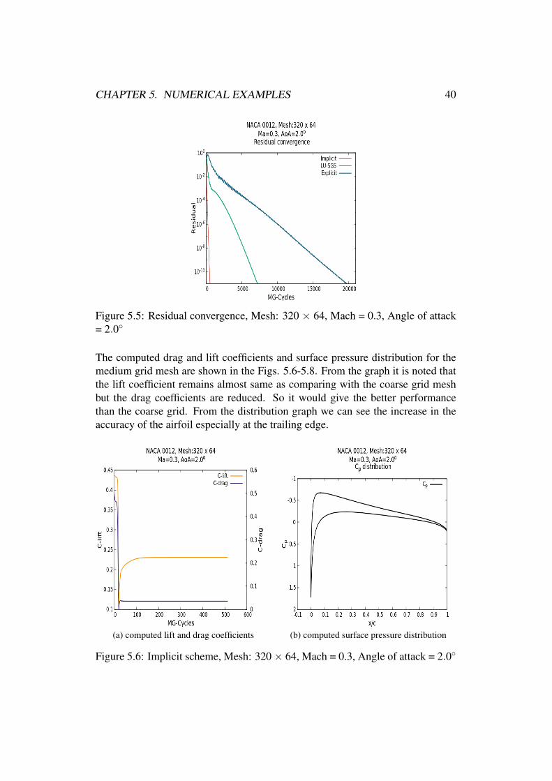
5.6 Implicit scheme, Mesh: 320 × 64, Mach = 0.3, Angle of attack =2.0 . . . . . . . . . . . . . . . . . . . . . . . . . . . . . . . . . 40
5.7 LU-SGS scheme, Mesh: 320 × 64, Mach = 0.3, Angle of attack= 2.0 . . . . . . . . . . . . . . . . . . . . . . . . . . . . . . . . 41
5.8 Explicit scheme, Mesh: 320 × 64, Mach = 0.3, Angle of attack =2.0 . . . . . . . . . . . . . . . . . . . . . . . . . . . . . . . . . 41
5.9 Residual convergence, Mesh: 640 × 128, Mach = 0.3, Angle ofattack = 2.0 . . . . . . . . . . . . . . . . . . . . . . . . . . . . . 42
5.10 Implicit scheme, Mesh: 640 × 128, Mach = 0.3, Angle of attack= 2.0 . . . . . . . . . . . . . . . . . . . . . . . . . . . . . . . . 43
5.11 LU-SGS scheme, Mesh: 640 × 128, Mach = 0.3, Angle of attack= 2.0 . . . . . . . . . . . . . . . . . . . . . . . . . . . . . . . . 43
5.12 Explicit scheme, Mesh: 640 × 128, Mach = 0.3, Angle of attack= 2.0 . . . . . . . . . . . . . . . . . . . . . . . . . . . . . . . . 44
5

LIST OF FIGURES 6
5.13 Residual convergence, Mesh: 160 × 32, Mach = 0.8, Angle ofattack = 1.25 . . . . . . . . . . . . . . . . . . . . . . . . . . . . 45
5.14 Implicit scheme, Mesh: 160 × 32, Mach = 0.8, Angle of attack =1.25 . . . . . . . . . . . . . . . . . . . . . . . . . . . . . . . . . 46
5.15 LU-SGS scheme, Mesh: 160 × 32, Mach = 0.8, Angle of attack= 1.25 . . . . . . . . . . . . . . . . . . . . . . . . . . . . . . . 46
5.16 Residual convergence, Mesh: 320 × 64, Mach = 0.8, Angle ofattack = 1.25 . . . . . . . . . . . . . . . . . . . . . . . . . . . . 47
5.17 Implicit scheme, Mesh: 320 × 64, Mach = 0.8, Angle of attack =1.25 . . . . . . . . . . . . . . . . . . . . . . . . . . . . . . . . . 48

List of Tables
4.1 Butcher Scheme . . . . . . . . . . . . . . . . . . . . . . . . . . . 28
5.1 Butcher Scheme for all computations . . . . . . . . . . . . . . . . 355.2 Iteration, Mesh: 160 × 32, Mach = 0.3, Angle of attack = 2.0 . . 375.3 Iteration, Mesh: 320 × 64, Mach = 0.3, Angle of attack = 2.0 . . 395.4 Iteration, Mesh: 640 × 128, Mach = 0.3, Angle of attack = 2.0 . 425.5 Iteration, Mesh: 160 × 32, Mach = 0.8, Angle of attack = 1.25 . 455.6 Iteration, Mesh: 320 × 64, Mach = 0.8, Angle of attack = 1.25 . 47
7


Chapter 1
Introduction
Iterative solution methods are often used to approximate solutions of nonlinearequations. For this to be done we need to linearize the nonlinear equation byapproximating the derivative and then make use of any iterative method to ap-proximately solve the linear equation. This approximate solution is used to up-date the state of the outer nonlinear iteration. PDE or integral equations are oftendiscretized and solved approximately by the following way: Mesh generation,Governing Equation, Discretization, Algorithm implementation, comparison ofresults.
In the Mesh generation step meshes are generated. But in our thesis we are notgoing to generate the mesh, instead we are going to use the already generatedmesh of NACA0012 airfoil. Read the available grid file, which means calculationof number of elements, faces, edges, etc. and calculation of normal, surface area,etc. The elements in the mesh are triangle and quadrilateral, that is a hybrid orunstructured mesh.
The Governing equation step deals with the integral form of the Euler equation inconservative form, that is the unknowns are represented as conservative variables.Then the next step is very important to address the main issues of the discretiza-tion of the integral equations. All the algorithms and their required functions forsolving the Euler equation are discussed in Solution algorithm step. In our thesisthe used solution algorithms are implicit scheme, LU-SGS scheme and explicitscheme. The Implicit and LU-SGS scheme are differentiated by approximatingthe derivative of the residual and the LU-SGS scheme is reduced to a single stage.The explicit scheme is the straight forward method. Then in the Numerical exam-ples step we can be able to plot and compare our results with different test cases.Finally we can give the conclusion of the current work and small introductionabout future work.
8

Chapter 2
Governing Equations
2.1 Governing equations in integral formIn this section we are going to represent the governing equations, which are re-quired for this thesis and are referred from the lecture notes [1]. Let us considerthe bounded domain Ω⊂ R2. The governing equations are derived from the fun-damental laws of conservation of mass, momentum and energy. The first namedas the conservation of mass.
ddt
∫Ω
ρ(x, t)dx +∫
∂Ω
〈(ρu)(x, t),n〉 ds = 0. (2.1a)
The second named as the conservation of momentum.
ddt
∫Ω
(ρu)i(x, t) dx +∫
∂Ω
〈(ρu)i(x, t) u(x, t) + P(x, t)ei,n〉 ds = 0. (2.1b)
The third named as the conservation of Energy.
ddt
∫Ω
(ρE)(x, t) dx +∫
∂Ω
〈ρ(x, t)H(x, t)u(x, t),n〉 ds = 0. (2.1c)
The quantities ρ(x, t), u(x, t) = (u1(x, t),u2(x, t))T , E(x, t) and
H(x, t) := E(x, t)+P(x, t)/ρ(x, t) (2.2)
are density, velocity, the specific total energy and the enthalpy of the fluid. n isthe unit outward normal. P is the pressure defined by the state equation given as
P(x, t) := (γ−1)ρ(x, t)(
E(x, t)− ‖u‖22
2
), (2.3)
γ is the gas-dependent ratio of specific heat, which is given by 1.4 for air.
9

CHAPTER 2. GOVERNING EQUATIONS 10
2.2 Integral form of euler equationLet us consider the domain to describe the flow effects Ω ⊂ R2, i.e., an openand connected set, and an integral [0,T ) ⊂ R, T > 0, the RANS equations inconservative form. The fundamental laws of conservation of mass, momentumand energy resulting a system of non-linear conservation laws. The governingequations can be expressed in the general form as
ddt
VΩ(W )(t)+R∂Ω(W )(t) = 0, t ∈ [0,T ) (2.4a)
where the integral operators VΩ and R∂Ω are given by
VΩ(W )(t) :=∫
Ω
W (x, t) dx. (2.4b)
For Euler equation,
R∂Ω(W )(t) :=∫
∂Ω
〈 fc(W ),n〉 ds, (2.4c)
where W (x, t) is the conservative variable,
W (x, t) =
ρ(x, t)
ρ(x, t)u1(x, t)ρ(x, t)u2(x, t)ρ(x, t)E(x, t)
,
The term fc(W ) describes the convective contribution
fc(W ) :=
ρu
(ρu1)u+Pe1(ρu2)u+Pe2
ρHu
,
and 〈 fc(W ),n〉 is called the convective flux in normal direction n, which is givenby
〈 fc(W ), n〉=
ρ(x, t)V
(ρu1)(x, t)V +P(x, t)n1(ρu2)(x, t)V +P(x, t)n2
ρ(x, t)H(x, t)V
,
where,
V := 〈u(x, t),n〉= u1n1 +u2n2 (2.5)

CHAPTER 2. GOVERNING EQUATIONS 11
describes the normal velocity. The speed of sound is denoted as a, dimensionlessMach number is denoted as M are defined by
a :=
√γPρ, M :=
‖u‖22
a. (2.6)
The speed of sound a can be reformulated by using the equation of state as
a2 = (γ−1)(
H− ‖u‖22
2
).
Equation (2.4a) is rewritten as,
ddt
∫Ω
W (x, t) dx+∫
∂Ω
〈 fc(W ),n〉 ds = 0, (2.7)
which is the integral form of the Euler equation.
2.3 Governing equations in differential formThe integral equation (2.7) hold for any infinitely small sub domain, here (2.4a)holds for any small domain and for the whole domain one can obtain the differen-tial form, to reformulate the equations 2.1a, 2.1b, 2.1c into differential form, weapply Gauss-Divergence theorem.
Gauss-Divergence theorem is given as∫Ω
div fc(W )dx =∫
∂Ω
〈 fc(W ),n〉ds. (2.8)
The fundamental laws of conservation of mass, momentum and energy in differ-ential form can be rewritten as,∫
Ω
∂ρ(x, t)∂ t
dx +∫
Ω
div((ρu)(x, t))dx = 0, (2.9a)
∫Ω
∂
∂ t(ρu)i(x, t)dx +
∫Ω
[div((ρui)(x, t)u(x, t))
+ div(P(x, t)ei)]dx = 0,(2.9b)
∫Ω
∂
∂ t(ρE)(x, t)dx +
∫Ω
div(ρ(x, t)H(x, t)u(x, t))dx = 0. (2.9c)

CHAPTER 2. GOVERNING EQUATIONS 12
Equation 2.9a - 2.9c hold for all bounded, open subset Ω, one obtains the differ-ential equations
∂
∂ tρ(x, t) +
2
∑j=1
∂
∂x j(ρu)(x, t) = 0, (2.10a)
∂
∂ t(ρui)(x, t) +
2
∑j=1
(∂
∂x j(ρuiu j)(x, t) + δi j
∂
∂x jP(x, t)
)= 0, (2.10b)
∂
∂ t(ρE)(x, t) +
2
∑j=1
∂
∂x j(ρ(x, t)H(x, t)u(x, t)) = 0. (2.10c)
2.4 Differential form of euler equationThe differential form of the Euler equation, which is derived from the integralequation is given as
∂
∂ tW (x, t)+div fc(W ) = 0 (2.11)
where W (x, t) is the conservative variable, fc(W ) is the convective term describedin the Section 2.2.

Chapter 3
Discretization
3.1 Computational MeshThis section deals about computation of the meshes, which are referred from thelecture notes [1]. Let us assume that the bounded computational domain is cov-ered by a given finite set of domains Ωii=1,...Nelem .
Let Ω ⊂ R2 be a bounded domain. Assume that there exists a finite set of opendomains Ωii=1,...Nelem , Ωi ⊂ R2, Ωi 6= /0, covering Ω, that is
Ωi ⊂Ω, Ω =Nelem⋃i=1
Ωi, Ωi∩Ω j = /0, i 6= j.
Then the set
M := Ω : i = 1, ...,Nelem
is called a mesh or a grid or a decomposition covering Ω.
For two dimensional case, the decomposition M is called feasible if for all i 6= jeither Ωi∩Ω j = /0 or one of the following conditions hold:
a) Ωi∩Ω j 6= /0 and Ωi and Ω j share exactly one corner, or
b) Ωi∩Ω j 6= /0 and Ωi and Ω j share exactly one edge, or
A feasible decomposition M of Ω⊂R2 is called a triangulation or a finite volumemesh. It is noted that the considered meshes consist of triangles and quadrilateralsonly.
13

CHAPTER 3. DISCRETIZATION 14
3.1.1 Common Definitions(a) The volume of Ω is denoted by
vol(Ω) :=∫
Ω
1 dx.
(b) The point x ∈ R2 is called barycenter of Ω
xi :=1
vol(Ω)
∫Ω
yi dx, i = 1,2.
(c) If edge(face) is defined as Ωi∪ (R2 \Ω) 6= 0, then the boundary edge(face)is defined as
ei,bdry := Ωi∪ (R2 \Ω).
(d) The surface area of the face ei j is denoted by
svol(ei j) :=∫
∂Ωi∩Ω j
1 ds.
(e) The surface area of the boundary face ei,bdry is denoted by
svol(ei,bdry) :=∫
∂Ωi∩(R2\Ω)1 ds.
(f) The outer unit normal vector of the face ei j is denoted by
nei j = ni j = (n1,i j,n2,i j).
(g) The outer unit normal vector of the face ei,bdry is denoted by
nei,bdry = ni,bdry = (n1,i,bdry,n2,i,bdry).
3.1.2 Computation of area/volume of triangleLet us consider the element Ω be a triangle with coordinates [P1, P2, P3] asshown in Fig. 3.1. From the available general definition in the section 3.1.1 thearea/volume of the triangle is computed mathematically as follows

CHAPTER 3. DISCRETIZATION 15
P1
P2
P3
Figure 3.1: Area of triangle
vol(Ω) =12[(XP1−XP2)(YP1 +YP1)+(XP2−XP3)(YP2 +YP3)
+(XP3−XP1)(YP3 +YP1)].
3.1.3 Computation of area/volume of quadrilateralLet us consider the element Ω be a quadrilateral with coordinates [P1, P2, P3, P4]as shown in Fig. 3.2. From the available general definition in the section 3.1.1 thearea/volume of the quadrilateral is computed mathematically as follows
P1
P2
P3
P4
Figure 3.2: Area of quadrilateral
vol(Ω) =12[(XP4−XP2)(YP1 +YP3)+(XP1−XP3)(YP2 +YP4)].
3.2 DiscretizationAs we mentioned in the introduction part, this is one of the important steps forthis thesis referred from [1]. So let us consider the differential form of the Euler

CHAPTER 3. DISCRETIZATION 16
equation,∂
∂ tW (x, t)+div fc(W ) = 0, (3.1)
multiplying the suitable test function v, apply the Gauss Divergence theorem andidentity, which is given below to the equation (3.1)
div(v fc(W )) = vdiv( fc(W ))+ 〈 fc(W ),gradv〉,
we will get the weak form of Euler equation as∫Ω
vdWdt
dx−∫
Ω
〈gradv, fc(W )〉dx+∫
∂Ω
〈v fc(W ),n〉ds = 0. (3.2)
Equation (3.2) holds for all possible test functions v. In this thesis we are going todo finite volume discretization, in which we approximate the unknown functionW representing it by a sum of constant ansatz functions. For this purpose we aregoing to define the indicator function, which is described as follows
1Ωi(x) :=
1, x ∈Ωi0, else
and W is approximated by using the constant function Wh,
W (x, t)≈Wh(x, t)≈Nelem
∑i=1
Wi(t)1Ωi(x),
it is always the case that,
grad(Wi1Ωi)|Ωi = 0, i = 1, ...,Nelem
so, now the only test function is
v(x) =Nelem
∑i=1
1Ωi(x), i = 1, ...,Nelem
As we know our test function is a constant function, which gives gradv(x) = 0.And we substitute all those in our weak form of Euler equation (3.2), then we ar-rive with the discretized form of Euler equation with finite volume discretization,which is given as follows
Nelem
∑i=1
(vol(Ωi)
dWi
dt+∫
∂Ωi
〈 fc(Wh),n〉ds)= 0. (3.3)
To do the discretization we need the quadrature formula for the volume and sur-face integrals. But the surface integrals lead us into the trouble when the vector W

CHAPTER 3. DISCRETIZATION 17
of the conserved variable is discontinuous across the faces. These problems arenamed as Riemann problems and to address these issues the concept of a numeri-cal flux function has been introduced, which is the stable numerical method in theup-winding scheme. These flux functions are also often called as Riemann solver.Hence the surface integral in equation(3.3) is written as follows,∫
∂Ωi
〈 fc(Wh),n〉ds = ∑j∈N(i)
∫ei j
H(WL(i,N(i)),WR( j,N( j)), n)ds, (3.4)
where H is the numerical flux function and the neighbors of the vertex i and j aredenoted by N(i) & N( j) respectively. Here, WL(i,N(i)) and WR( j,N( j)) are thefunctions, which is used to compute the flux over the face ei j are not only baseddirectly on the Wi, Wj, but also on the neighbor stencil. In detail the states arereconstructed as follows,
WL(i,N(i)) =W (Wi,Wk,k∈N(i)), WR( j,N( j)) =W (Wj,Wk,k∈N( j))
As stated before the state WL may depend on the coefficient vector Wi and allthe surrounding coefficient vectors Wk, k ∈ N(i), and similarly the state WR maydepend on the coefficient vector Wj and all the surrounding coefficient vectors Wk,k ∈ N( j). Hence the equation with the approximation of surface integral is givenas, ∫
ei j
〈 fc(Wh),n〉ds ≈ svol(ei j)H(WL(i,N(i)),WR( j,N( j)), nei j),
where surface area of the face ei j is already defined in Section 3.1.4. In our casewe are considering only the fluxes corresponding to the direct neighbors. So themodified equation is given as,∫
ei j
〈 fc(Wh),n〉ds ≈ svol(ei j)H(Wi,Wj, nei j).
The numerical flux function in normal direction n by corresponding to a first orderRoe scheme is defined as
H1st,Roe(Wi,Wj,n) :=12[〈 fc(Wi),n〉 + 〈 fc(Wj),n〉] −
12|ARoe
i j |(Wj−Wi). (3.5)
The operator ARoei j is given by
ARoei j :=
∂ 〈 fc(Wi j,Roe),n〉∂W
,

CHAPTER 3. DISCRETIZATION 18
here ’Roe’ refers that we use Roe averaged variables to evaluate the correspondingterm on the edge (face) i j,
ρi j,Roe :=√
ρiρ j, (3.6a)
(ui j,Roe)k :=(ui)k√
ρi +(u j)k√
ρ j√ρi +√
ρ j, k = 1,2 (3.6b)
Hi j,Roe :=Hi√
ρi +H j√
ρ j√ρi +√
ρ j, (3.6c)
a2i j,Roe := (γ−1)
(Hi j,Roe −
12
∥∥ui j,Roe∥∥2
2
), (3.6d)
Ei j,Roe := Hi j,Roe −a2
i j,Roe
γ. (3.6e)
Equation (3.6d) represents square of the corresponding Roe averaged speed ofsound and equation (3.6e) represents the total energy.
3.3 Discretization of boundary conditionsAll boundary conditions considered here are implemented using a flux formula-tion [2]. The used boundary condition in our thesis are given as,
1. Farfield boundary condition
2. Slip wall boundary condition
Figure 3.3: Examples of primary mesh

CHAPTER 3. DISCRETIZATION 19
The flux over the edge ei,bdry needs to satisfy the corresponding boundary con-dition using flux formulations. Here the coefficients Wi of the ansatz functioncorresponding to the element Ωi are given. In order to compute the flux we needto define an an outer artificial state, which is given as
Wi,bdry =
(ρi,bdry(t),(ρu)i,bdry(t),(ρE)i,bdry(t)
)T
.
This outer artificial state should satisfy the boundary condition for the boundaryedge ei,bdry and the approximated boundary integral can be given by,
∫∂Ωi
〈 fc(W ), n〉 ds≈Nbdry
∑i=1
∫ei,bdry
H1st,Roe (Wi,Wi,bdry,ni,bdry) ds
≈Nbdry
∑i=1
svol (ei,bdry) H1st,Roe (Wi,Wi,bdry,ni,bdry).
3.3.1 Farfield boundary conditionUsing this boundary condition we can find the inflow of free-stream conditions ofthe fluid. For the given angle of attack α , the outer state can be found by
Wi,bdry :=W∞ := (ρ∞, cosαρ∞u∞, sinαρ∞u∞, ρ∞E∞)T .
3.3.2 Slip wall boundary conditionThe slip wall boundary conditions are used for the inviscid flow problem. Toensure a vanishing normal velocity the outer state can be found by
ρi,bdry := ρi,
(ρu)i,bdry := (ρu)i−2〈(ρu)i,ni,bdry〉ni,bdry,
ρi,bdryEi,bdry := ρiEi.
3.4 Derivative of the convective fluxIn this part we are going to do the implementation of the Matrix Dissipation,which is referred from the paper ”Investigation and application of point implicitRunge-Kutta methods to inviscid flow problems” [3]. Here the determination ofthe eigenvalues and eigenvectors does not require rewriting the derivative in prim-itive variables and convert it back. With this there is an advantage of adding theturbulent parts if it is necessary in future. But in our thesis we are not looking

CHAPTER 3. DISCRETIZATION 20
for any turbulent parts and formulation of Matrix Dissipation can be implementedstraightforward.
Let us consider the convective part of equation (2.4), mentioned in the page 10,
〈 fc(W ),n〉=V
ρ
ρu1ρu2ρE
+P
0n1n20
+V P
0001
=VW +P
0n1n2V
.
Now the derivative of 〈 fc(W ),n〉 is given by
∂ 〈 fc(W ),n〉∂W
=V I +W∂V (W )
∂W+
0n1n2V
∂P(W )
∂W+P
000
∂V (W )
∂W
. (3.7)
The derivative of the normal velocity, V = 〈u,n〉 is given by
∂V (W )
∂W=
1ρ
−Vn1n20
T
. (3.8)
Apply equation 3.8 in 3.7
∂ 〈 fc(W ),n〉∂W
=V I +1ρ
ρ
ρu1ρu2ρE
(−V,n1,n2,0)+
000pρ
(−V,n1,n2,0)+
0n1n2V
∂P(W )
∂W
(3.9a)
=V I +
1u1u2H
(−V,n1,n2,0)+
0n1n2V
∂P(W )
∂W. (3.9b)
Now we need derivation of pressure P, which is given by
∂P(W )
∂W= (γ−1)
(‖u‖2
22
,−u1,−u2,1). (3.10)

CHAPTER 3. DISCRETIZATION 21
Let us write the full matrix of derivative of fc. n by applying equation 3.10 in 3.9b
∂ 〈 fc(W ),n〉∂W
=
V 0 0 00 V 0 00 0 V 00 0 0 V
+−V n1 n2 0−Vu1 u1n1 u1n2 0−Vu2 u2n1 u2n2 0−V H Hn1 Hn2 0
+
0 0 0 0
γ−12‖u‖2
2 n1 −(γ−1)u1n1 −(γ−1)u2n1 (γ−1)n1
γ−12‖u‖2
2 n2 −(γ−1)u1n2 −(γ−1)u2n2 (γ−1)n2
γ−12‖u‖2
2V −(γ−1)u1V −(γ−1)u2V (γ−1)V
∂ 〈 fc(W ),n〉∂W
=
0 n1 n2 0
n1ζ2 ‖u‖22
2−u1V n1ζ3u1 +V n2u1−n1ζ2u2 n1ζ2
n2ζ2 ‖u‖22
2−u2V n1u2−n2ζ2u1 n2ζ3u2 +V n2ζ2
(ζ2 ‖u‖22− γE)V n1ζ1−ζ2u1V n2ζ1−ζ2u2V γV
(3.11)
where
ζ1 = γE−Φ, ζ2 = γ−1, ζ3 = 2− γ, Φ =12(γ−1)‖u‖2
2
3.5 Eigenvalues and Eigenvectors of the derivativeof the convective flux
We define the vectors
a1 := (1,u1,u2,H)T
a2 := (0,n1,n2,V )T
b1 := (−V,n1,n2,0)T
b2 :=(
∂P(W )
∂W
)T
Then using Equation 3.9b the derivative of the convective flux can be assembledas
∂ 〈 fc(W ),n〉∂W
=V I +a1bT1 +a2bT
2 . (3.12)

CHAPTER 3. DISCRETIZATION 22
Then we notice that x ∈R4 is eigenvector with eigenvalue V of∂ ( fc.n)(W )
∂Wif and
only if the orthogonality relations
bT1 x = bT
2 x = 0 (3.13)
hold. It can be easily verified that the vectors
y1 =
1u1u2
‖u‖22
, y2 =
0n2−n1
n2u1−n1u2
, y3 =
0−n2n1
n1u2−n2u1
,
satisfy equation 3.13. However the vectors y2,y3 are linearly dependent since
y2 + y3 = 0.
Two linear-independent eigenvectors may be obtained as
g1 := Ay1 +ay2
g2 := Ay1 +ay3
where a :=√
γPρ
denotes the speed of sound and A :=√
n21 +n2
2 denotes the sur-
face area. In our case we have used the normal, which is normalized by surfacearea, so the value of surface area is equal to 1. To identify the remaining eigen-vectors we use the relations
bT1 a1 = bT
2 a2 = 0, bT1 a2 = A2 and bT
2 a1 = a2, (3.14)
bT1 a1 = (−V,n1,n2,0)
1u1u2H
=−V +u1n1 +u2n2 = 0,
where, V is defined in equation (2.5) . similarly bT2 a2 = 0.
bT1 a2 = (−V,n1,n2,0)
1n1n2V
= n21 +n2
2 = A2,

CHAPTER 3. DISCRETIZATION 23
bT2 a1 = (γ−1)
(‖u‖2
22
,−u1,−u2,1)
1u1u2H
=γPρ
= a2.
Then we compute using Equation(3.12)
∂ 〈 fc(W ),n〉∂W
(Aa1 +aa2) =V I(Aa1 +aa2)+a1bT1 (Aa1 +aa2)+a2bT
2 (Aa1 +aa2)
=VAa1 +Vaa2 +Aa1bT1 a1 +aa1bT
1 a2 +Aa2bT2 a1 +aa2bT
2 a2
=VAa1 +Vaa2 +0+aa1A2 +Aa2a2 +0
=VAa1 +Vaa2 +aa1A2 +Aa2a2
= (V +aA)(Aa1 +aa2)
similarly,
∂ 〈 fc(W ),n〉∂W
(Aa1−aa2) =VAa1 +a2Aa2−Vaa2−A2aa1
= (V −aA)(Aa1−aa2)
Hence we found the two additional eigenvalues V + aA and V − aA with corre-sponding eigenvectors g3 := Aa1 +aa2 and g4 := Aa1−aa2.
3.6 Eigendecomposition of the derivative of the con-vective flux
The eigendecomposition of the derivative of the convective flux is given as
∂ 〈 fc(W ),n〉∂W
= G Λ G−1 (3.15)

CHAPTER 3. DISCRETIZATION 24
Where Λ is a diagonal matrix, which has on its diagonal the eigenvalues of∂ 〈 fc(W ),n〉
∂W
and columns of matrix G are the eigenvectors of∂ 〈 fc(W ),n〉
∂W
G = (g1,g2,g3,g4)
Λ =
VV
V +aAV −aA
We define the vectors
P1 :=γ−1
a2
H−‖u‖2
2u1u2−1
(3.16a)
P2 :=
u1n2−u2n1−n2n10
(3.16b)
P3 :=
u2n1−u1n2
n2−n1
0
(3.16c)
and
q1 :=1
2A2
(ApT
1 −1a
PT2
)(3.17a)
q2 :=1
2A2
(ApT
1 −1a
PT3
)(3.17b)
q3 :=1
2a2A
(bT
2 +aA
bT1
)(3.17c)

CHAPTER 3. DISCRETIZATION 25
q4 :=1
2a2A
(bT
2 −aA
bT1
)(3.17d)
Then the inverse of G is given by
J :=
q1q2q3q4
i.e. G−1 = J
Here we are going to use some of the important equations
PT1 y1 =
γ−1a2
(H−‖u‖2
2 +‖u‖22−‖u‖2
22
)=
γ−1a2
(H−‖u‖2
2
)= 1,
PT1 y2 = PT
1 y3 = PT2 y1 = PT
3 y1 = 0,
PT2 y2 =−n2
2−n21, PT
3 y3 =−n22−n2
1,
PT2 y3 = n2
2 +n21, PT
3 y2 = n22 +n2
1,
bT1 y1 = bT
1 y2 = bT1 y3 = 0,
bT2 y1 = bT
2 y2 = bT2 y3 = 0,
and equation (3.14) to prove the assertion
q1g1 =1
2A2
(A2PT
1 y1−Aa
PT2 y1 +aAPT
1 y2−PT2 y2
)=
12A2 (A
2 +n21 +n2
2) = 1,
q1g2 = q1g3 = q1g4 = 0,
q2g2 =1
2A2
(A2PT
1 y1−Aa
PT3 y1 +aAPT
1 y3−PT3 y3
)=
12A2 (A
2 +n21 +n2
2) = 1,
q2g1 = q2g3 = q2g4 = 0,
q3g3 =1
2a2A
(AbT
2 a1 +abT1 a1 +abT
2 a2 +a2
AbT
1 a2
)=
12a2A
(a2A+a2A) = 1,
q3g1 = q3g2 = q3g4 = 0,
q4g4 =1
2a2A
(AbT
2 a1−abT1 a1−abT
2 a2 +a2
AbT
1 a2
)=
12a2A
(a2A+a2A) = 1,
q4g1 = q4g2 = q4g3 = 0.
3.7 Entropy fixFor a construction of the stable scheme, it is important to use the so-called entropyfix. Entropy fix is to avoid the instabilities when one of the eigenvalues is ≈ 0.

CHAPTER 3. DISCRETIZATION 26
Let λ1,λ2,λ3,λ4 be the eigenvalues, then the entropy fix is described as follows,
λ1 := max|V |,δ (|V |+aA),λ2 := max|V |,δ (|V |+aA),λ3 := max|V +aA|,δ (|V |+aA),λ4 := max|V −aA|,δ (|V |+aA),
where δ is the user defined value. In our case we are using δ = 0.2. Note that ifthe choice of δ = 0, then no entropy fix is used.
Finally, we obtain equation (3.3) as given below
dWdt
=−M−1 R(W ), where M := diag(vol(Ωi)i=1,..,Nelem). (3.18)
We are only interested in approximating a steady state solution of equation (3.18).Hence the above equation is simplified as
−M−1 R(W ) = 0 (3.19)

Chapter 4
Solution Algorithms
Nonlinear multigrid: solves R(W ) = 0
Requires: Sequence of meshes, Smoother, Interpolation and Projection operator
Runge-Kutta smoother: computes W (n+1) =W (n)+P−1R(W (n))
Requires: Derivative, Linear solver
Krylov subspace method: solves Ph = R
Requires: Efficient preconditioner
Linear Preconditioner: solves Prec w = Pv
Requires: Efficient iterative linear solver
Linear Multigrid
Requires: Sequence of meshes oralgebraic multigrid, Smoother,
Interpolation and Projection
Figure 4.1: Algorithmical structure of nonlinear solution method
A general graphical overview to construct a powerful algorithm to solve a non-linear equation is given in Figure 4.1, which is referred from [1]. It shows theconnection of several required inputs. In our thesis the nonlinear algebraic system
27

CHAPTER 4. SOLUTION ALGORITHMS 28
of equations of interest is given by equation (3.19).
We can apply nonlinear multi grid method using an implicit Runge-Kutta smootherto solve the algebraic system of equations approximately and efficiently. Then wewill get linear system of equations, they are solved approximately by using oneof the iterative solution methods. We have to make use of the preconditioner toapproximate efficiently a solution of the linear systems. To approximately solveefficiently the linear system linear multi grid methods can be applied.
4.1 Point implicit Runge-Kutta methodTo solve the discretized flow equation (3.19) we consider multi stage diagonallyimplicit Runge-Kutta method given by the Butcher scheme (Table 4.1). Referredfrom the Journal ”Aglomeration multigrid methods with implicit Runge-Kutta smoothersapplied to aerodynamic simulations on unstructured grids” [4].
c AbT
Table 4.1: Butcher Scheme
where,
A :=
α11 0 . . . 0
α21. . . . . . ...
... . . . . . . 00 . . . αs,s−1 αss
, b :=
0...0
αs+1,s
and c :=
0...0
(4.1)
The stages of the implicit Runge-Kutta scheme and discrete evolution are givenby
k1(W ) =−M−1R(W Tn +α11∆tk1(W )),
k2(W ) =−M−1R(W Tn +α21∆tk1(W )+α22∆tk2(W )),
...
ks(W ) =−M−1R(W Tn +αs,s−1∆tks−1(W )+αss∆tks(W )),
W Tn+1 =W Tn +αs+1,s∆tks(W ). (4.2)

CHAPTER 4. SOLUTION ALGORITHMS 29
To approximate a solution of nonlinear systems k1, . . . ,ks we use one iteration ofthe Newton’s method to approximate the root of the function
g j(k j(W )) := k j(W )+M−1R(W Tn +α j, j−1∆tk j−1(W )+α j j∆tk j(W )).
And its derivative is given by
∂g j(k j(W ))
∂k j(W )[k j(W )] = I+α j j∆tM−1 ∂R
∂W(W Tn +α j, j−1∆tk j−1(W )+α j j∆tk j(W )),
and with an assumed initial guess k(0)j (W ) = 0 the approximate root is given by
k j(W ) =−[Pj(W )]−1(g j(k(0)j (W ))), (4.3)
where
Pj(W ) = I+α j j∆tM−1 ∂R∂W
[W Tn +α j, j−1∆tk j−1(W )].
Using these formulas the implicit Runge-Kutta method (4.2), where the innerNewton iteration is truncated after one step, can be represented by the algorithm
k1(W ) =−[P1(W )]−1M−1R(W Tn),
k2(W ) =−[P2(W )]−1M−1R(W Tn +α21∆tk1),
...
ks(W ) =−[Ps(W )]−1M−1R(W Tn +αs,s−1∆tks−1),
W Tn+1 =W Tn +αs+1,s∆tks(W ).
Substitute W (0) :=W Tn and
W ( j) :=W Tn−α j+1, j∆t[Pj(W )]−1M−1R(W ( j−1))
Now the implicit Runge-Kutta method is reformulated as
W (0) :=W Tn,
W (1) :=W (0)−α21∆tP1(W )−1M−1R(W (0)),
... (4.4)
W (s) :=W (0)−αs+1,s∆tPs(W )−1M−1R(W (s−1)),
W Tn :=W (s).
Algorithm (4.4) indicates that for each stage the linear equation
Pj(W )h j = α j+1, j∆tM−1R(W ( j−1))
needs to be solved. This can be equivalently formulated by((∆t)(−1)M+α j j
∂R∂W
)h j = α j+1, jR(W ( j−1)). (4.5)

CHAPTER 4. SOLUTION ALGORITHMS 30
4.2 Construction of preconditionerAs described in the section 3.2, an appropriate first order discretization is used to
approximate the the exact derivative∂R∂W
. We are here neglecting the second order
terms and assuming ARoei j as locally constant, the derivative of the convective flux∫
∂Ωifc.n ds is formulated as,
∂Ri
∂Wk=
12
∑ j∈N(i) |ARoe
i j |, k = i,−|ARoe
i j |, k ∈ N(i),0, k 6= i, k 6∈ N(i).
(4.6)
We can simplify it further based on approximating terms of the first-order Jaco-bian by their spectral radius [5]. Equation (3.5) is replaced by a first-order scalardissipative term,∫
∂Ωi
fc.n ds≈ ∑j∈N(i)
12[〈 fc(Wi),n〉 + 〈 fc(Wj),n〉] −
12
ρ(ARoei j )(Wj−Wi) (4.7)
and ρ(ARoei j ) denotes the spectral radius of ARoe
i j . Corresponding to Equation (4.6),the derivative of the convective flux is
∫∂Ωi
fc.n ds approximated by
∂Rscalari
∂Wk=
12
∑ j∈N(i)ρ(ARoe
i j ), k = i,−ρ(ARoe
i j ), k ∈ N(i),0, k 6= i, k 6∈ N(i).
(4.8)
Then for steady state computations the time step ∆t in equation 4.5 is replaced by∆T := diag(diag(∆ti)), where
∆ti := CFL.vol(Ωi)
[∑
j∈N(i)
12(|Vi j|+ai jsvol(ei j))
]−1
(4.9)
Finally equation 4.5 is replaced by((∆T )(−1)M+α j j
∂R∂W
)h j = α j+1, jR(W ( j−1)) (4.10)
From the above equation the final preconditioner is given as
Prec j := (∆T )−1M+α j j∂R∂W
(W ( j−1)) (4.11)
Precscalarj := (∆T )−1M+α j j
∂Rscalar
∂W(W ( j−1)) (4.12)

CHAPTER 4. SOLUTION ALGORITHMS 31
4.3 Iterative solution methods for linear equationsIn order to approximate efficient solution of the above linear equation (4.10)we are going to use any of the iterative solution methods like (Block) Jacobi or(Block) Gauss-Seidel [4]. Let Pi j denotes the entries of the preconditioner, thenBlock Jacobi method and Block Gauss-Seidel method are given as follows,
hk+1i = (Pi,i)
−1(
bi−Nelem
∑j=1, j 6=i
Pi, jh(k)j
)for i = 1, . . . ,Nelem, (4.13)
hk+1i = (Pi,i)
−1(
bi−i−1
∑j=1
Pi, jh(k+1)j −
Nelem
∑j=i+1
Pi, jh(k)j
)for i = 1, . . . ,Nelem.
(4.14)
It is noted that in our code we are realizing our (Pi,i)−1 by using the pivoted LU
decomposition.
4.4 Efficient smootherIn order to obtain low-cost efficient smoother our algorithm(4.6) reduces to theapproximate solution of
Prec jh j = α j+1, j R(W ( j−1)), (4.15)
and as a consequence Algorithm simplifies to
W (0) :=W n,
W (1) :=W (0)−α21Prec−11 R(W (0)),
... (4.16)
W (s) :=W (0)−αs+1,sPrec−1s R(W (s−1)),
W n+1 :=W (s).
It can also be the case that we can use the freezing preconditioner Prec on the firststage, that is
W (0) :=W n,
W (1) :=W (0)−α21Prec−11 R(W (0)),
... (4.17)
W (s) :=W (0)−αs+1,sPrec−11 R(W (s−1)),
W n+1 :=W (s).

CHAPTER 4. SOLUTION ALGORITHMS 32
Assuming that the operator Prec j, j = 1, . . . ,s, do not change significantly overone Runge-Kutta iteration and that the construction of Prec j together with thecomputation of the block LU-decomposition of th TriGi is a time consuming ap-proach, this simple frozen Runge-Kutta iteration may yield an efficient solution.
4.5 LU-SGS schemeConsidering the algorithm (4.4) as a smoother and Precscalar
j is constructed asdescribed in the Section 4.2. Then for each stage in algorithm, we need to solvethe linear system
Precscalarj h j = α j+1, jR(W ( j−1)), (4.18)
rewriting our preconditioner as,((∆T )−1M+α j j
∂Rscalar
∂W(W ( j−1))
)= (L+D+U),
where L denotes the lower, D denotes the diagonal, and U denotes the upper partof the matrix. To approximately solve the above equation efficiently, we apply onesymmetric Gauss-Seidel sweep. Because of one symmetric Gauss-Seidel sweepour equation can be rewritten as,
(D+L)D−1(D+U)h j = α j+1, jR(W ( j−1)). (4.19)
And choosing only one stage in the algorithm (4.4), the resulting scheme is knownas LU-SGS scheme.
4.6 Explicit Runge-Kutta accelerated by local timestepping
Considering the algorithm (4.4) as a smoother and Prec j is constructed as de-scribed in the section 4.2 with α j j = 0. Then for each stage in algorithm, we needto solve the linear system,
h j = ∆T M−1R(W ( j−1)).
Approximately solving the linear system by the application of block Jacobi methodand choosing the proper stopping criteria, we get exactly a solution algorithm de-noted as explicit Runge-Kutta accelerated by local time stepping and the algorithm

CHAPTER 4. SOLUTION ALGORITHMS 33
can be written as follows,
W (0)i :=W n,
W (1)i :=W (0)−CFLexpα21
∆tiMi
Ri(W (0)),
... (4.20)
W (s)i :=W (0)−CFLexpαs+1,s
∆tiMi
Ri(W (s−1)),
W n+1i :=W (s).

Chapter 5
Numerical Examples
In the following section we will show examples with different test cases, in whichthe solution methods that we discussed in the previous section are used. We wouldlike to test our algorithm for a subsonic and a transonic flow. The test cases are asfollows,
(a) Inviscid flow over the NACA 0012 airfoil at the inflow Mach number, Ma =0.3 and angle of attack of 2.0 using the solution algorithms Implicit schemebased on a derivative corresponding to a discretization of compact stencil,LU-SGS scheme and Explicit Runge-Kutta accelerated by local time step-ping on coarse grid mesh (160 × 32).
(b) Inviscid flow over the NACA 0012 airfoil at the inflow Mach number, Ma =0.3 and angle of attack of 2.0 using the solution algorithms Implicit schemebased on a derivative corresponding to a discretization of compact stencil,LU-SGS scheme and Explicit Runge-Kutta accelerated by local time step-ping on medium grid mesh (320 × 64).
(c) Inviscid flow over the NACA 0012 airfoil at the inflow Mach number, Ma =0.3 and angle of attack of 2.0 using the solution algorithms Implicit schemebased on a derivative corresponding to a discretization of compact stencil,LU-SGS scheme and Explicit Runge-Kutta accelerated by local time step-ping on fine grid mesh (640 × 128).
(d) Inviscid flow over the NACA 0012 airfoil at the inflow Mach number, Ma =0.8 and angle of attack of 1.25 using the solution algorithms Implicit schemebased on a derivative corresponding to a discretization of compact stenciland LU-SGS scheme on coarse grid mesh (160 × 32).
(e) Inviscid flow over the NACA 0012 airfoil at the inflow Mach number, Ma =0.8 and angle of attack of 1.25 using the solution algorithm Implicit scheme
34

CHAPTER 5. NUMERICAL EXAMPLES 35
based on a derivative corresponding to a discretization of compact stencilon medium grid mesh (320 × 64).
In our computations we have chosen the Butcher scheme as,
0 1 0 0
03
201 0
0 025
1
0 0 1
Table 5.1: Butcher Scheme for all computations
We are going to use the CFL ramping strategy to choose the CFL number, whichis given as
CFL(n) = minCFLinit . f (n), CFLmax (5.1a)
f (n) =
1, n < 10,γn−10, n≥ 10
(5.1b)
The parameters CFLinit, CFLmax, γ are given in the description of the examples.The residuals are computed by a volume weighted norm, normalized with respectto the evaluated with free stream values, which is named as density residual andis given by,
density residual(n) :=
√√√√ N
∑j=1
(R j,ρ(W n))2
vol(Ω j)2
/√√√√ N
∑j=1
(R j,ρ(W∞))2
vol(Ω j)2 (5.2)
All the computations are stopped when the density residual has dropped 12 ordersof magnitude or number of iteration has reached 20000, and this is the stoppingcriteria for all the test cases. We have used 5 symmetric sweeps in the Gauss-Seidal method and preconditioner is not frozen on the multi stage Runge-Kuttascheme.
In order to investigate the examples we additionally compute the well establishedaerodynamic scalar values and distributions, which is referred from [2]. The scalarvalues are
1. drag coefficient CD

CHAPTER 5. NUMERICAL EXAMPLES 36
2. lift coefficient CL
The drag and lift coefficients are defined as follows
CD(W ) :=2
ρ∞u2∞
⟨∫∂Ω
〈 fc(W ), n〉 ds(y), g(α)
⟩(5.3)
and
CL(W ) :=2
ρ∞u2∞
⟨∫∂Ω
〈 fc(W ), n〉 ds(y), h(α)
⟩(5.4)
where, g(α) := (0,cosα,sinα,0)T and h(α) := (0,−sinα,cosα,0)T in which α
is the angle of attack.
For an inviscid flow we can calculate the CD and CL only by the contributionof forces corresponding to the pressure. Similarly we can calculate the surfacepressure distribution Cp also, which is defined as
p(W (x)) :=⟨〈 fc(W ), n〉 ds(y), (0,n(x),0)T
⟩, x ∈ ∂Ω, (5.5)
Cp(W (x)) :=2
ρ∞u2∞
(p(W (x))− p∞), x ∈ ∂Ω, (5.6)
5.1 Test case (a)We consider an inviscid flow over the NACA 0012 airfoil at the inflow Mach num-ber, Ma = 0.3 and angle of attack of 2.0. We perform the computations using allthe three solution algorithms on the mesh of dimension 160 × 32.
Let us assume CFLinit = 1, CFLmax = 1000 and γ = 1.2. These numbers areused only for Implicit and LU-SGS scheme. For Explicit scheme we chooseCFLexp = 0.75. The comparison of all the three schemes based on the conver-gence history of the residuals are shown in the Fig. 5.1.

CHAPTER 5. NUMERICAL EXAMPLES 37
Figure 5.1: Residual convergence, Mesh: 160 × 32, Mach = 0.3, Angle of attack= 2.0
From the graph it is observed that the residual is converged very fast by using theimplicit scheme after that LU-SGS scheme converges and the explicit scheme isvery slower than the other two schemes. It is evident by seeing the CPU time. Forthe explicit scheme we can be able to note that there is some initial oscillations inthe graph. The detailed information of the iteration count and the CPU time aregiven in the Table 5.2.
Algorithm Implicit LU-SGS ExplicitNo. of iterations 288 3877 9574
CPU time in seconds 73.71 186.542 758.952
Table 5.2: Iteration, Mesh: 160 × 32, Mach = 0.3, Angle of attack = 2.0
The computed drag and lift coefficients and surface pressure distribution are shownin the Figs. 5.2-5.4. As expected the drag and lift coefficients and Cp distributionare same in all the algorithms except the initial oscillations of lift and drag coeffi-cients in explicit scheme. From the Cp distribution graph, it is noted that there isloss of accuracy and the trailing edge is not connected properly. That is becauseof the mesh density, we are using only the coarse grid (160 × 32).

CHAPTER 5. NUMERICAL EXAMPLES 38
(a) computed lift and drag coefficients (b) computed surface pressure distribution
Figure 5.2: Implicit scheme, Mesh: 160 × 32, Mach = 0.3, Angle of attack = 2.0
(a) computed lift and drag coefficients (b) computed surface pressure distribution
Figure 5.3: LU-SGS scheme, Mesh: 160 × 32, Mach = 0.3, Angle of attack =2.0

CHAPTER 5. NUMERICAL EXAMPLES 39
(a) computed lift and drag coefficients (b) computed surface pressure distribution
Figure 5.4: Explicit scheme, Mesh: 160 × 32, Mach = 0.3, Angle of attack = 2.0
5.2 Test case (b)We consider an inviscid flow over the NACA 0012 airfoil at the inflow Mach num-ber, Ma = 0.3 and angle of attack of 2.0. We perform the computations using allthe three solution algorithms on the mesh of dimension 320 × 64.
Let us assume the same CFL numbers as the previous test case. The comparisonof convergence history of the residuals for this test case are shown in the Fig. 5.5.Also from the CPU time it is seen that the implicit scheme converges faster thanthe other two schemes in the medium grid mesh also. And for the explicit schemethe oscillations are carried throughout the convergence but using the coarse gridit was only at the beginning. The detailed information of the iteration count andCPU time for the medium grid mesh are given in the Table 5.3.
Algorithm Implicit LU-SGS ExplicitNo. of iterations 512 7203 19803
CPU time in seconds 518.54 1274.72 6256.55
Table 5.3: Iteration, Mesh: 320 × 64, Mach = 0.3, Angle of attack = 2.0
CHAPTER 5. NUMERICAL EXAMPLES 40
Figure 5.5: Residual convergence, Mesh: 320 × 64, Mach = 0.3, Angle of attack= 2.0
The computed drag and lift coefficients and surface pressure distribution for themedium grid mesh are shown in the Figs. 5.6-5.8. From the graph it is noted thatthe lift coefficient remains almost same as comparing with the coarse grid meshbut the drag coefficients are reduced. So it would give the better performancethan the coarse grid. From the distribution graph we can see the increase in theaccuracy of the airfoil especially at the trailing edge.
(a) computed lift and drag coefficients (b) computed surface pressure distribution
Figure 5.6: Implicit scheme, Mesh: 320 × 64, Mach = 0.3, Angle of attack = 2.0

CHAPTER 5. NUMERICAL EXAMPLES 41
(a) computed lift and drag coefficients (b) computed surface pressure distribution
Figure 5.7: LU-SGS scheme, Mesh: 320 × 64, Mach = 0.3, Angle of attack =2.0
(a) computed lift and drag coefficients (b) computed surface pressure distribution
Figure 5.8: Explicit scheme, Mesh: 320 × 64, Mach = 0.3, Angle of attack = 2.0

CHAPTER 5. NUMERICAL EXAMPLES 42
5.3 Test case (c)We consider an inviscid flow over the NACA 0012 airfoil at the inflow Mach num-ber, Ma = 0.3 and angle of attack of 2.0. We perform the computations using allthe three solution algorithms on the mesh of dimension 640 × 128.
Let us assume the same CFL numbers. The comparison of convergence historyof the residuals for this test case are shown in the Fig. 5.9. Here also the im-plicit scheme converges faster, LU-SGS scheme converges slower but the explicitscheme never converges and the oscillations are very high. So we stopped when-ever the iteration reaches 20000. Being a straight forward method explicit schemeis taking too much of time to converge when we are using fine grid mesh. It isnoted that implicit scheme is working nice and it is taking very less number ofiterations and the CPU time is also very less. The detailed information of theiteration count and CPU time for the fine grid mesh are given in the Table 5.4.
Algorithm Implicit LU-SGS ExplicitNo. of iterations 957 13937 NA
CPU time in seconds 3910.30 9915.93 NA
Table 5.4: Iteration, Mesh: 640 × 128, Mach = 0.3, Angle of attack = 2.0
Figure 5.9: Residual convergence, Mesh: 640× 128, Mach = 0.3, Angle of attack= 2.0

CHAPTER 5. NUMERICAL EXAMPLES 43
(a) computed lift and drag coefficients (b) computed surface pressure distribution
Figure 5.10: Implicit scheme, Mesh: 640 × 128, Mach = 0.3, Angle of attack =2.0
(a) computed lift and drag coefficients (b) computed surface pressure distribution
Figure 5.11: LU-SGS scheme, Mesh: 640 × 128, Mach = 0.3, Angle of attack =2.0

CHAPTER 5. NUMERICAL EXAMPLES 44
(a) computed lift and drag coefficients (b) computed surface pressure distribution
Figure 5.12: Explicit scheme, Mesh: 640 × 128, Mach = 0.3, Angle of attack =2.0
The computed drag and lift coefficients and surface pressure distribution are shownin the Figs. 5.10-5.12. Using the fine grid mesh also we are having the same liftcoefficient but the drag coefficient is reduced further. Obviously the performanceis also increased with fine grid mesh. In the distribution graph also the accuracyhas increased and it is very much noted at the trailing edge of the airfoil.
5.4 Test case (d)We consider an inviscid flow over the NACA 0012 airfoil at the inflow Machnumber, Ma = 0.8 and angle of attack of 1.25. Here we are going to performthe computations only for the implicit and LU-SGS schemes on the mesh of di-mension 160 × 32. It is noted that we could not perform the computations for theexplicit scheme in this transient flow condition.
Let us assume CFLinit = 50, CFLmax = 1000 and γ = 1.2. In order to run ourcode for this test case we have to alter the CFL number initially. The comparisonof these schemes based on the convergence history of the residuals are shown inthe Fig. 5.13. From the graph it is observed that both the schemes are convergingbut the implicit scheme is quiet fast and stable compared to the LU-SGS scheme.It is also evident by seeing the CPU time. The detailed information of the iterationcount and CPU time are given in the Table 5.5.

CHAPTER 5. NUMERICAL EXAMPLES 45
Algorithm Implicit LU-SGSNo. of iterations 441 7332
CPU time in seconds 108.71 347.18
Table 5.5: Iteration, Mesh: 160 × 32, Mach = 0.8, Angle of attack = 1.25
Figure 5.13: Residual convergence, Mesh: 160× 32, Mach = 0.8, Angle of attack= 1.25
The computed drag and lift coefficients are shown in the Figs. 5.14 and 5.15. Boththe schemes are giving the same results in drag and lift coefficients.

CHAPTER 5. NUMERICAL EXAMPLES 46
Figure 5.14: Implicit scheme, Mesh: 160 × 32, Mach = 0.8, Angle of attack =1.25
Figure 5.15: LU-SGS scheme, Mesh: 160 × 32, Mach = 0.8, Angle of attack =1.25
5.5 Test case (e)We consider an inviscid flow over the NACA 0012 airfoil at the inflow Machnumber, Ma = 0.8 and angle of attack of 1.25. Here we are going to perform the

CHAPTER 5. NUMERICAL EXAMPLES 47
computations only for the implicit scheme on the mesh of dimension 320 × 64.
As discussed in the previous section we have to alter the CFL number initially,which is assumed as CFLinit = 100, CFLmax = 1000 and γ = 1.2. The conver-gence history of the residual is shown in the Fig. 5.16. It is noted that the implicitscheme is the only method available to run on the given mesh under the givencondition. From the graph it is seen that the scheme is converging smoother. Thedetailed information of the iteration count and CPU time are given in the Table5.6.
Algorithm ImplicitNo. of iterations 724
CPU time in seconds 718.19
Table 5.6: Iteration, Mesh: 320 × 64, Mach = 0.8, Angle of attack = 1.25
Figure 5.16: Residual convergence, Mesh: 320× 64, Mach = 0.8, Angle of attack= 1.25
The computed drag and lift coefficients are shown in the Fig. 5.17. By comparingit with the coarse grid mesh there exists marginal increase in the lift coefficientand drag coefficient is decreased. This would give us the better performance.

CHAPTER 5. NUMERICAL EXAMPLES 48
Figure 5.17: Implicit scheme, Mesh: 320 × 64, Mach = 0.8, Angle of attack =1.25

Chapter 6
Conclusion and Future work
From the observation of all the test cases in this thesis, we can find that the im-plicit scheme is giving the better performance than the other two schemes and itis fast and stable process also. Even LU-SGS scheme is also giving us the de-sired result but it is time consuming process. The derivative of the residual playsmajor role in it. As discussed in the solution algorithm chapter the derivative ofthe residual used in the implicit scheme includes the non diagonal elements also,that is the reason for the fast convergence. In LU-SGS scheme the derivative isapproximated only by the spectral radius and it is reduced to the single stage andthe explicit scheme is straight forward. By increasing the mesh density we obtainmore accurate results.
It is also noted that we can be able to perform computations using all the threeschemes on all the three meshes if the test cases are having the subsonic flowcondition (Ma = 0.3). But for the transonic flow condition (Ma = 0.8) we couldnot perform any calculation using the explicit scheme on our meshes, LU-SGSscheme on medium and fine grid meshes and implicit scheme on fine grid mesh.
In the future we can extend our work by adding some additional features to our al-gorithm that can really take care of these issues. Some of them are we can replaceour first order approximation by the second order approximation in the approx-imation of the derivative of our numerical flux. We can make use of multi gridalgorithm and we can also modify our iterative solution method, which is (Block)Gauss-Seidel, in which we can exploit to line information. It is always interestingto see the changes by altering something in the existing base system.
49

Bibliography
[1] S. Langer, Algorithmen zur Losung der Euler und Navier-Stokes Gleichungen.2017.
[2] S. Langer, Preconditioned Newton methods to approximate solutions of theReynolds averaged Navier-Stokes equations.
[3] S. Langer, “Investigation and application of point implicit runge-kutta meth-ods to inviscid flow problems,” International Journal for Numerical Methodsin Fluids, 2011.
[4] S. Langer, “Aglomeration multigrid methods with implicit runge-kuttasmoothers applied to aerodynamic simulations on unstructured grids,” Jour-nal of Computational Physics, 2014.
[5] S. Langer, “Investigation and comparison of implicit smoothers applied inagglomeration multigrid,” AIAA JOURNAL, 2015.
[6] S. Langer, “Implicit methods and globalization strategies for the robust ap-proximation of solution to the reynolds averaged navier-stokes equations,”
[7] S. Langer, “Hierarchy of preconditioning techniques for the olution of thenavier-stokes equations discretized by 2nd order unstructured finite volumemethods,”
50


![Performance Comparison of Several Folding …Performance Comparison of Several Folding Strategies Jim Newton[0000 0002 1595 8655] EPITA Research Lab, 94270 Le Kremlin Bec^etre, FRANCE](https://img.dokumen.tips/doc/110x75/5f19dca0bdb969471659bdee/performance-comparison-of-several-folding-performance-comparison-of-several-folding.jpg)