Embed Size (px)
Citation preview

Comparison of Radiofrequency Coil Configurations for Multiple
Mouse Magnetic Resonance Imaging
by
Marc Carias
A thesis submitted in conformity with the requirements
for the degree of Masters of Science
Medical Biophysics
University of Toronto
© Copyright by Marc Carias 2013
ii
Comparison of Radiofrequency Coil Configurations for Multiple
Mouse Magnetic Resonance Imaging
Marc Carias
Masters of Science
Marc Carias
University of Toronto
2013
Abstract
Multiple-mouse MRI (MMMRI) accelerates biomedical research by imaging multiple mice
simultaneously. To date, MMMRI has been explored in three ways: shielded transmit-receive
coils, shielded transmits coil with separate unshielded receive coils; and finally shielded transmit-
receive coils with independent gradient coils. However alternative transmit coil configurations and
possible benefits of eliminating shielding have not yet been explored. The goal of this thesis is to
test possible radiofrequency configurations with and without shielding for the purpose of
improving image quality for MMMRI. Results demonstrate that using an unshielded transmit-
receive coil array provided a 20% improvement over an identical shielded coil. A new unshielded
7-coil MMMRI array is presented, minimizing the ghosting between image overlap using mutual
inductance minimization and a sensitivity encoding (SENSE) reconstruction. The final array
provided high resolution images (90µm) of up to seven live mice simultaneously with appropriate
signal-to-noise for automated analysis.

iii
Acknowledgments
First and foremost I would like to acknowledge and thank my supervisor Dr. Brian Nieman for his
constant motivation and support during my thesis. He has introduced and taught me skills that
cannot be memorized or listened to in lecture. This allowed me to grow not only as a scientist but
also as an individual.
I would also like to thank my committee members, Dr. Mark Henkelman and Dr. Alex Vitkin.
Both their expertise and ability to ask the right questions guided my thesis to have a larger impact.
Their guidance and feedback pushed me to become a better student and become more familiar with
various topics.
The Mouse Imaging Centre deserves a special thanks, for providing a great work environment
filled with many areas of expertise. In particular I would like to personally thank Jun Dazai, the
mechanical engineer at MICe. With his help, intuition and motivation, I was able to efficiently
finish my thesis and acquire new skills in device design and machining. I would like to thank
Shoshana Spring, Christine LaLiberté and Dr. Lindsay Cahill for all the help with mouse handling
and support. Finally at MICe I would like to thanks Dr. Jonathan Bishop for his help with MR
sequencing and Michael Wong for some coding support and constant motivation.
I also acknowledge all the funding agencies including the Natural Sciences and Engineering
Research Council of Canada, OICR, and the Faculty of Medicine at University of Toronto.

iv
Table of Contents Chapter One - Introduction
1.1 Mouse Imaging ......................................................................................................................... 1
1.2 MRI ........................................................................................................................................... 2
1.2.1 Fundamentals of MRI Theory ............................................................................................ 2
1.2.2 Radiofrequency Coils ......................................................................................................... 3
1.3 Parallel Imaging ........................................................................................................................ 6
1.3.1 Surface Coils ...................................................................................................................... 6
1.3.2 Phased Array ...................................................................................................................... 7
1.3.3 Sensitivity Encoding .......................................................................................................... 9
1.4 MMMRI and Parallel Imaging ............................................................................................... 12
Chapter Two - Experiments
2.1 Saddle Coil Design ................................................................................................................. 14
2.1.1 Methods ............................................................................................................................ 15
2.1.2 Results ............................................................................................................................. 17
2.2 MMMRI Configurations ......................................................................................................... 20
2.2.1 Methods ............................................................................................................................ 21
2.2.2 Results .............................................................................................................................. 22
2.3 The Effect of Shielding ........................................................................................................... 23
2.3.1 Methods ............................................................................................................................ 24
2.3.1 Results .............................................................................................................................. 24
2.4 Receive Geometries and Coupling ......................................................................................... 25
2.4.1 Rotation ............................................................................................................................ 26
2.4.2 Translation ........................................................................................................................ 28
2.4.3 Depth ................................................................................................................................ 30
2.4.4 Coupling and SNR ........................................................................................................... 32
2.4.4.1 Methods ..................................................................................................................... 32
2.4.4.2 Results ....................................................................................................................... 32
2.5 Theoretical Design of a MMMRI Array ................................................................................. 34
2.6 Imaging with the array ............................................................................................................ 39
2.6.1 Methods ............................................................................................................................ 40
v
2.6.2 Results .............................................................................................................................. 41
Chapter Three - MMMRI Coil Array
3.1 Benefits ................................................................................................................................... 44
3.2 Potential Use ........................................................................................................................... 45
3.3 Custom Coils ........................................................................................................................... 46
3.4 Summary ................................................................................................................................. 48

vi
List of Tables
Table 1 - Orientations (in degrees) of Two Saddle Coils
vii
List of Figures
Figure 1 - Simple Resonant Circuit
Figure 2 - SNR Measurements using Regions of Interest
Figure 3 - Surface Coil Schematic with Field Simulation
Figure 4 - Geometric Decoupling Between Coils
Figure 5 - Sensitivity Encoding Reconstruction
Figure 6 - Saddle Coil Schematic with Parameters
Figure 7 - B1 Profile of a Saddle Coil
Figure 8 - SNR Measurements of Various Saddle Coils
Figure 9 - Saddle Coil Form and Actual Photo
Figure 10 - Radiofrequency Configurations Schematics
Figure 11 - SNR Results of RF Configurations
Figure 12 - Shielding of RF Coils
Figure 13 - SNR and Mutual Inductance of Rotating Saddle Coils
Figure 14 - SNR and Mutual Inductance of Translating Saddle Coils
Figure 15 - SNR and Mutual Inductance of Shifting Saddle Coils
Figure 16 - Comparing SNR and Mutual Inductance
Figure 17 - Mutual Inductance Minimization Results
Figure 18- B1 Field Maps of coils 1 through 4 within the Array
Figure 19 - Saddle Coil Orientation Sensitivity
Figure 20 - CAD drawing and Actual Photo of Final Array
Figure 21 - Pre and Post SENSE Phantom Images
Figure 22 - 7 Live Mice Brain Images Post SENSE Reconstructed
Figure 23 - Three dimensional average image of 7 live mice brains
Figure 24 - Custom Intubated Mouse Imaging Coil and Holder

viii
List of Acronyms
MMMRI - Multiple Mouse MRI
SENSE - Sensitivity Encoding
MICe - Mouse Imaging Centre
OICR - Ontario Institute for Cancer Research
SNR - Signal to Noise Ratio
RF - Radiofrequency
CAD - Computer-aided Design
MRI - Magnetic Resonance Imaging
Tx - Transmit
Rx - Receive
Tx-Rx - Transmit receive
ID - Inner Diameter
OD - Outer Diameter
M - Mutual Inductance
FOV - Field of View
ROI - Region of Interest
TR - Repetition Time
TE - Echo Time
BOLD - Blood Oxygen Level Dependant
3D - Three dimensional
ASL - Arterial Spin labelling
CBV - Cerebral Blood Volume

1
Chapter 1
Introduction
This thesis will focus on comparing different radiofrequency coil configurations for in vivo
multiple mouse MRI. The introduction will begin with a brief section on mouse imaging, followed
by a brief introduction to basic MRI. A more detailed section is provided for radiofrequency coils
and using multiple coils to gain sensitivity in a phased array. This chapter will conclude with a
discussion on current techniques for multiple mouse MRI followed by the motivation for this
thesis.
1.1 Mouse Imaging
Mice in a laboratory can be manipulated and analyzed in a fashion that cannot take place in human
studies. For instance, genetic models, in which genes are added to or removed from the genome,
can be created to study the resulting phenotype (observable characteristics or traits) (1-3). In
addition, diseases such as cancer can be followed longitudinally over their full time course when
using mouse models (4-6). Magnetic resonance imaging (MRI) can be a powerful tool in the
analysis of mouse models by providing an in vivo imaging modality that offers soft tissue contrast
and high resolution capability (7-11). Compared to clinical imaging, high field strengths and longer
scan times are necessary in order to obtain sufficient resolution for mouse imaging. Mouse studies
always require statistical analysis of findings. This is efficiently achieved through increasing the
number of samples within a study. Therefore, there is a need for more effective imaging throughput
(8).

2
A typical small animal MRI system may accomplish two to four live imaging sessions a day. The
duration of each scan is limited by the length of time mice can spend under anesthesia, typically a
max of 3 hours. However by using a multiple-mouse MRI (MMMRI) technique as described in
Bock et al. (8,9), one can accomplish relatively high throughput (up to 16 mice at once) without
sacrificing signal to noise (10,11). This is achieved by using a larger magnet than necessary for a
single mouse and imaging multiple mice simultaneously using independent shielded RF coils. Due
to the high resolution needed in mouse MRI, much importance is still placed in maximizing
efficient use of image signal.
1.2 MRI
1.2.1 Fundamentals of MRI Theory
The basis of MRI is the directional magnetic moment associated with spin 1/2 nuclei. When a
sample is placed in a large magnetic field, a very slight majority of the free hydrogen moments
align themselves with the direction of the magnetic field. This creates a net magnetization aligned
with the main magnetic field (B0) (20). If perturbed from this position, the net magnetization
precesses about the main magnetic field, like a gyroscope. This behavior is termed Larmor
precession (20). The rate of precession is given by the Larmor equation, Eq. 1.
[1]
This introduces a parameter γ, known as the gyromagnetic ratio which is specific to different
nuclei. The precessing magnetization generates electromagnetic radiation that can be detected and
used for MRI. Equation 1 allows calculation of the frequencies of spins in this magnetic field for
MRI (20). For example, at 7 Tesla the hydrogen atom resonates at 300 MHz.
002
Bf
3
There are two steps in acquiring MRI signals. First, the net magnetization must be perturbed from
its equilibrium along the main magnetic field. This is achieved using a radiofrequency (RF) field
that is perpendicular to the main field and operating at the Larmor frequency, known as the B1
field. This rotates the net magnetization about B0. The RF coil in this case is called a transmit coil
and the process is sometimes referred to as transmission. After transmission, the precession of the
net magnetization must be detected. The precessing magnetization induces current in a receiver
coil that is oriented to detect magnetization perpendicular to B0. Afterwards, the signal from the
receive coil is amplified and digitized. The RF receive and transmit functions can be performed
using the same or separate coils.
1.2.2 Radiofrequency Coils
RF coils are responsible for transmission and reception and therefore can be thought of as the
MRI’s antenna. This is achieved via an electrical circuit containing a series of capacitors (C) and
inductors (L, inherent to coil geometry) (25,26) (figure 1A). At resonance the two impedances of
C and L are of equal magnitude. In a very simple model (figure 1) the resonance frequency is given
by Eq. 2 (26). In an MRI system the impedance is typically matched to 50 Ohms, to accommodate
the back end electronics so no losses (reflections) occur. In order to accomplish this, a matching
network (Fig. 1B) is placed on the coil. Here, R, L and Cs represent coil components where R is
the resistance of the coil (copper wire), L, the coil inductance (dependent on size, shape and coil
geometry) and Cs the series capacitance. Many separate series capacitors can be used to reduce
the effective inductance of the coil or coil element (capacitive segmentation) (21). The matching
network contains two components, a variable tuning capacitor (Ct) and a variable matching
capacitor (Cm). Ct creates a parallel resonance and allows tuning of the coil.

4
Figure 1: RF coils for acquiring MRI signals can be modeled by using a series of inductors (L), capacitors (C) and
resistors (R) in a circuit. A. Simple LC resonant circuit for Eq. 2 to achieve the desired resonance at a given
frequency. B. Most types of RF coils for small animal imaging can be modeled with this circuit. It contains three
capacitors, Cs, Ct (variable tuning), and Cm (variable matching), an inductor L (representing total coil inductance), a
resistor (representing all inherent coil resistance) and the measured voltage V.
𝜔0 =1
√𝐿𝐶= 2𝜋𝑓0 [2]
Since the RF coil is responsible for both transmission and reception, much importance is placed
on the design and efficiency of these coils to obtain the highest signal-to-noise ratio (SNR)
possible. SNR can be measured as the average signal within a region of interest in an imaged
sample divided by the standard deviation of the background signal noise, which in MRI is
Gaussian-distributed in the complex image and Rician-distributed in the magnitude image (figure
2). In practice, to maximize sensitivity in RF coil design, the coil is designed to maximize the
magnetic field (B1) produced per unit current over the desired region of space. The principle of
reciprocity (24) ensures that this design will also maximize current induced by a source within the
same region. With an increase in sensitivity of the coil, the SNR of images generally also increases
(21-23). The increase in SNR achieved, if present, will depend upon the dominant noise sources
affecting the image. Noise can be generated within the coil (thermal noise in the copper wire and
components) and from the sample (e.g., tissues within the body). Both sources degrade image
5
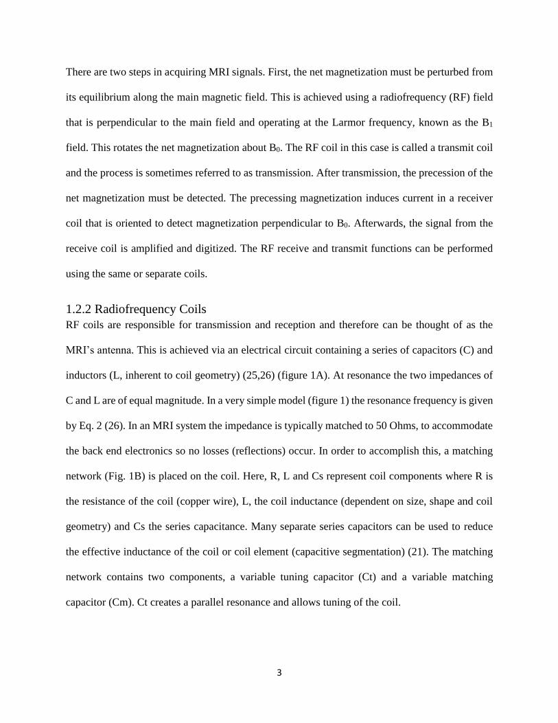
quality identically. With respect to coil design, only the sensitivity to sample signal and the coil
noise generated can be altered, which must be maximized and minimized respectively (21, 23).
Figure 2: SNR is used as a measure of image quality in MRI. SNR is measured by dividing the total average signal
intensity within a region of interest (black box, A), by the standard deviation of background noise (white box, B).
This method is how SNR was calculated throughout the thesis.
Whether coil noise or sample noise will be dominant for a given arrangement is determined by the
loading factor (Lf), Eq.3. The loading factor measures the difference in the electrical properties of
the circuit when a sample is placed within the coil versus an empty coil (21).
[3]
[4]
Lf can be determined from the quality factors (Q factor), Eq.4, of the empty coil (Qunloaded) and the
coil loaded with a sample (Qloaded). The Q factor is a metric that describes how the energy in a
resonant circuit dissipates relative to its initial energy. It is calculated as the resonant frequency
(ω0) quantity divided by the width (Δω) of the resonance at half the impendence's (magnitude)
maximum. When the loading factor (Lf) is below 0.5 the coil noise is expected to be greater than
unloaded
loaded
Q
QLf 1
0Q

6
the sample noise and improvements to the coil design will provide an increase in the SNR of the
image.
1.3 Parallel Imaging
1.3.1 Surface Coils
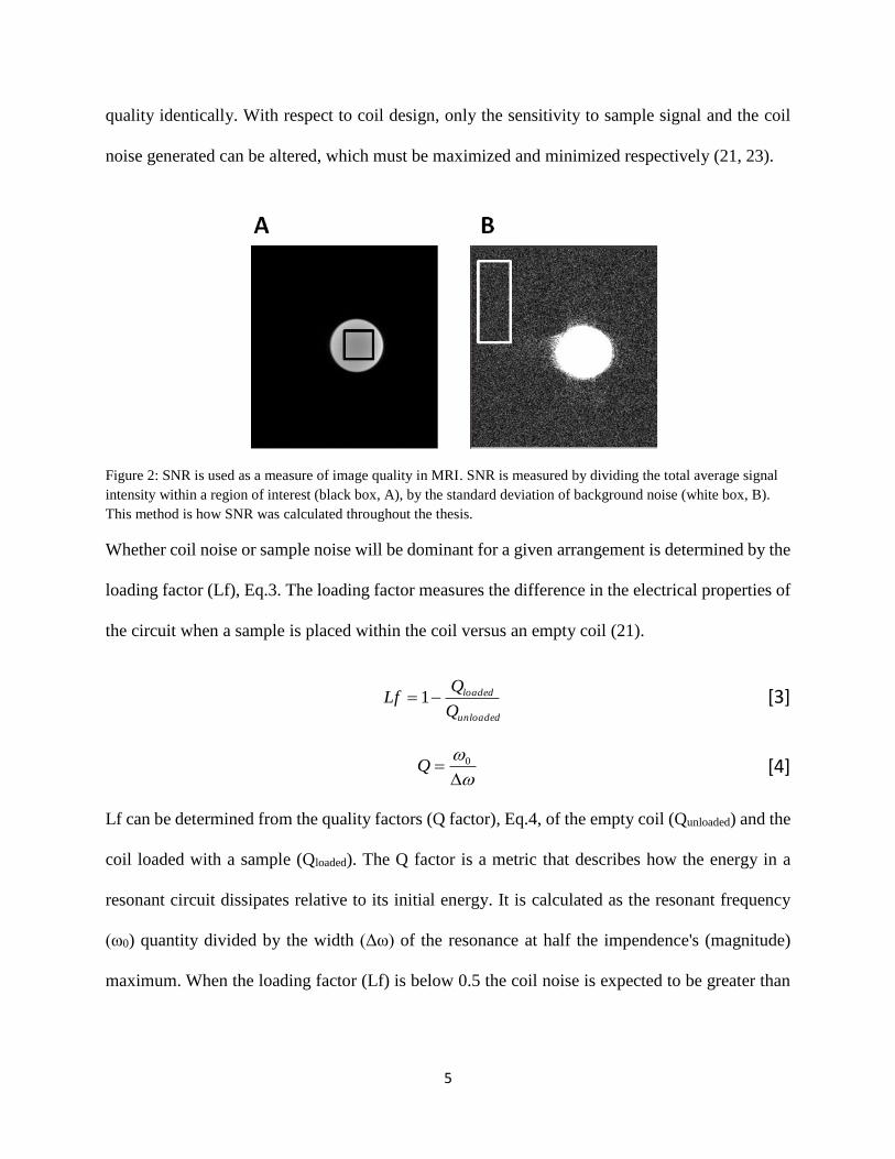
There are many types of coils with different geometries. Surface coils are one of the most common
in the clinic, where more than one are typically used to gain higher sensitivity. A surface coil is a
loop of wire that lays on the surface of a sample. They are typically used for their simplicity and
their ability to acquire high localized SNR (23,27,29). Figure 3 contains a surface coil schematic
with B1 direction drawn and calculated magnetic field map. A surface coil's effective area where
high SNR is acquired is a function of its radius (27-29), corresponding to the green to red colours
(larger than 50%) in figure 3B. For example a 12mm diameter surface coil will have a high SNR
up to ~6mm from the surface. Features below this will have poorer SNR and therefore a different
coil or multiple coils must be used. Additionally, RF coils should ideally be able to provide a
homogeneous B1 field (induced transmission field) throughout the sample (21). Unfortunately
surface coils are not homogenous. Therefore, one typically uses a surface coil for receive only,
and a separate transmit coil (volume coil) to achieve a homogeneous B1 field.
7
Figure 3: Surface coils, the most common RF coils, offer high local SNR however intensity quickly decreases as you
move away from the surface. A. A schematic indicating the direction of the created magnetic field (B1)
perpendicular to the surface coil. B. Simulated B1 map of a centre slice (grey plane shown in A), normalized to the
max intensity (simulation explained in section 2.1.1).
1.3.2 Phased Array
An array of receiver coils that encompasses an area of interest is called a phased array coil (15).
For this to occur, each receive coil must be connected to its own preamplifier and receive channel.
Currently, most new magnetic resonance systems are equipped with 16-32 channels in order to
accommodate phased arrays. When operating a phased array, several challenges need to be
overcome: Transmit (Tx)- receive (Rx) interactions need to be minimized (also a concern for a
single receive coil) (30), Rx-Rx interactions must be minimized (15), and a single image must be
reconstructed using data from all channels.
Allowing for separate Tx and Rx does provide homogeneous B1 with local sensitivity. However,
since the two coils are tuned to the same resonant frequency (f0), coupling can occur and decrease
the sensitivity. During Tx, induced currents in the Rx coil generate B1-fields that destroy the
desired homogeneity in the Tx-field (21). During Rx, since both coils must be resonant at f0, they
can couple into one another and act together like a large single coil, eliminating any local
sensitivity from the Rx coil. Strong coupling splits the coils' resonant peaks such that neither coil
has high sensitivity at f0 (15) (Figure 4).

8
Coupling must be kept at a minimum such that homogeneity is preserved and resonance splitting
does not occur. Geometric decoupling can be used to minimize both these interactions. The main
interaction between Tx-Rx and Rx-Rx coils is mutual inductance. Mutual inductance (M) is a
phenomenon where a change in current in a coil (while acquiring the MR signal) causes a change
in flux (the amount of magnetic field that passes through a surface) in an adjacent coil. It is
expressed by the Neumann formula (Eq.5):
𝑀 =𝜇0
4𝜋∯
𝑑𝑠𝑖∙𝑑𝑠𝑗
|𝑅𝑖𝑗| [5]
where, µ0 is the magnetic constant, followed by the line integrals of the two coils with a dot product
of coil elements (ds) divided by the distance between those coil elements (Rij) (31). Therefore one
can minimize M geometrically through coil orientation or distance. Optimal geometrical
decoupling between coils can be achieved when the magnetic flux of one coil does not pass through
any adjacent coils (15). This can be accomplished by either separating the coils or finding an
orientation where M sums to zero (figure 4). It was shown by Roemer et al. (15) that overlapping
surface coils does allow for decoupling, where the flux of adjacent coils do not interfere with others
(in this case net flux from one coil into another sums up to zero). For example, in a square surface
coil, an overlap of 10% of its length eliminates the double resonance phenomena (15).

9
Figure 4: Geometric decoupling occurs between RF coils when the flux of an adjacent coil does not induce current
in the other, by either summing to zero or being positioned orthogonally. A. No decoupling method between
adjacent coils. The results in a double peaked resonance (displayed as impedance magnitude) where no peak occurs
at f0. B. Two overlapped coils (green and yellow) where flux is eliminated in an adjacent coil through geometric
decoupling. This eliminates the double peak and resonance is restored at f0. This is shown in the figure where fields
from the green coil (red) that enter the yellow coil (fields not shown) sum to zero (both enter and leave, shown by
arrows) thus no coupling occurs.
1.3.3 Sensitivity Encoding
Once sufficient decoupling has been achieved between multiple Rx coils, a method is required to
reconstruct an image from the multiple channels of data. Figure 5 schematically demonstrates the
acquisition and reconstruction process often referred to as Sensitivity Encoding (SENSE) (16). For
a single coil and a fully sampled dataset, the acquired image (Ia) is the product of the coil sensitivity
(Ca1) and the object (ρ1), for every pixel in the image and coil sensitive region, Eq. 6.

10
𝐼𝑎 = 𝐶𝑎1𝜌1 [6]
It is common practice when using SENSE to acquire data from multiple coils and to sample less
data to reduce acquisition time. This has the effect of aliasing the image on top of itself. Each pixel
now contains information from several points in the object, ρ1-4, and signal from other pixels. It
can be written as (Eq. 7):
𝐼𝑎 = 𝐶𝑎1𝜌1 + 𝐶𝑎2𝜌2 + 𝐶𝑎3𝜌3 + 𝐶𝑎4𝜌4 [7]
In this equation, Ia is known (acquired), all four coil sensitivities are known (Ca), however all four
object pixels are unknown. If multiple receiver coils are introduced, with their own known
sensitive regions, corresponding equations here will be introduced per coil (figure 5). Therefore,
if we introduced three more coils (coils b, c and d) we have the dataset represented in Eq. 8 or 9:
𝐼𝑎 = 𝐶𝑎1𝜌1 + 𝐶𝑎2𝜌2 + 𝐶𝑎3𝜌3 + 𝐶𝑎4𝜌4
𝐼𝑏 = 𝐶𝑏1𝜌1 + 𝐶𝑏2𝜌2 + 𝐶𝑏3𝜌3 + 𝐶𝑏4𝜌4
𝐼𝑐 = 𝐶𝑐1𝜌1 + 𝐶𝑐2𝜌2 + 𝐶𝑐3𝜌3 + 𝐶𝑐4𝜌4 [8]
𝐼𝑑 = 𝐶𝑑1𝜌1 + 𝐶𝑑2𝜌2 + 𝐶𝑑3𝜌3 + 𝐶𝑑4𝜌4
Or
𝐼 = �̂� ∙ �⃗� [9]
The full image can be reconstructed using Eq. 10 (16) (figure 5):
�⃗� = �̂�−1 ∙ 𝐼 [10]
In order to obtain an accurate coil sensitivity map, a large field of view image is acquired to
determine a sensitivity map for each coil over the whole object. This sensitivity map includes the
spatial sensitivity inherent to the coil geometry and any residual coupling between coils. It is
important to obtain an accurate sensitivity map, so several post processing steps are usually

11
performed to reduce noise in the map. For example, since a smooth coil sensitivity is expected, we
can smooth the results using a polynomial fit to achieve an accurate map (16). In work described
in section 2.6 of this thesis, we will take the coil sensitivity C to be piecewise constant over
multiple samples in an array. This allows a very simple form of SENSE as described in Bock et
al. (8), referred to as a SENSE-like reconstruction. Note that this makes the assumption that the
dominant source of signal in the sensitivity map is residual coupling between coils. In this mode,
the key objective of SENSE is to separate coils signals from one another. This has the benefit of
also subtracting any noise likewise coupled, so can also improve SNR.
A measure known as the coil geometry factor tells us how well the SENSE method may separate
pixel intensities to corresponding images or how much our sensitivity maps overlap/relate with
one another (16) (Eq.11):
𝑔 =𝑆𝑁𝑅𝑐𝑜𝑖𝑙
𝑆𝑁𝑅𝑟𝑒𝑐𝑜𝑛 [11]
The g factor is computed by dividing the SNR of the initial coil image by the final reconstructed
image with all other coils present. The larger the g factor, the more coil sensitivities overlap.
SENSE is commonly used in clinical systems where there is often an excess of SNR that could be
traded off for lower scan time. This is not the case for mouse and small animal imaging where
extra sensitivity is usually desired to increase resolution.

12
Figure 5: SENSE reconstruction without artifact relies on accurate individual coil sensitivity maps to reconstruct the
desired image. Here, four surface coils are used to acquire an image. Each pixel in these images (Ia-d) contains
spatial data from four points in the object (ρ1-4). Using coil sensitivity maps (Ca-d1-4) at corresponding pixel
locations, equation 9 can be solved to acquire the desired reconstructed image.
1.4 MMMRI and Parallel Imaging
The aim in MMMRI is to generate separate images for many samples simultaneously. Initially
four configurations for performing MMMRI were considered (8). These included, i) imaging mice
with separate receivers and separate gradient coils, ii) imaging with separate unshielded RF coils
with a common gradient with a field of view (FOV) encompassing all mice, iii) imaging with
separate shielded RF coils with a common gradient with a small FOV and iv) imaging with separate
shielded RF coils with a common gradient with a large FOV. It was shown that using an individual
shielded RF coil per mouse with a common gradient coil (small FOV) allowed the highest
throughput without sacrificing image quality (8). A shield is a conductive material that surrounds
13
the RF coil to limit RF signal within a desired volume. This made it possible to run several
independent experiments in a single imaging session. It was later shown that this configuration
provides 3.3 times greater SNR when compared to imaging all samples in a single large image
with a large RF coil (12). A different approach has been described as a 'super-parallel microscope'
which introduces a separate gradient field per sample in a multiple imaging sample session (19).
A historic limitation of MMMRI is the availability of having multiple channels for transmit and
receive. Traditionally, MRI scanners were equipped with only one or two transmit channels,
favoring the large single transmit receive RF coil configuration, a major limitation for imaging
mice efficiently. However, this is no longer a challenge as most MRI systems are installed with
multiple channels (13,14). This dramatically increases the feasibly of implementing MMMRI,
which may allow it to become more common practice, even on human clinical systems.
Increasing the sensitivity of MMMRI has recently been investigated by adapting a multi-coil
interface to allow for parallel imaging or increased sensitivity. A multi-coil MMMRI (three receive
and one transmit coil per mouse) has recently been demonstrated and showed an acceleration factor
of 1.8 compared to the same image quality obtained using a single channel configuration (18). This
now allows receive coil arrays to be tailored to MMMRI experiments as seen in clinical systems
(14,18). However, possible transmit configurations with respect to image quality have not been
explored. Furthermore, SENSE and similar algorithms to separate signal from multiple coils are
now commonly used. This suggests that additional MMMRI configurations without shielding
between mice are possible, and they may have some image quality benefits. It is therefore the goal
of this thesis to explore possible radiofrequency coil configurations with and without shielding for
the purpose of improving image quality for MMMRI.

14
Chapter 2
Experiments
This chapter will focus on experiments conducted to determine a RF coil configuration for
MMMRI. I begin with an experiment involving the design of a RF coil specifically for in vivo
mouse brain imaging. Afterwards several RF configurations are compared using this newly
designed coil, accompanied by a discussion and further experiments involving shielding. Once a
configuration was chosen, I explored methods of geometric decoupling for design of a final array.
This chapter concludes with the construction of the final multiple mouse brain imaging array and
high resolution brain images of seven live mice.
2.1 Saddle Coil Design
At first I designed a volume coil capable of imaging the mouse brain with high sensitivity. A
volume coil is classified as a RF coil that encompasses a specific region of a sample with a fairly
uniform field over the region of interest, for example the head. Volume coils offer excellent
homogeneity compared to surface coils (15). The most effective volume coils are solenoids, which
offer the highest SNR and have excellent homogeneity (32,33). Solenoids are helical wound wires
with a number of turns around a cylinder that produces a magnetic field along the helical axis
(32,33). However, a major disadvantage of solenoids is that they must be positioned 90 degrees
relative to the main magnetic field B0. This constraint makes solenoids impractical for loading
live mice. A solution to the loading issue is to use a saddle coil. A saddle coil has a cylindrical
body coaxial with the magnet and turns of wire on the cylinders curved frame. The field produced
is perpendicular to the axis of the cylinder (figure 6).

15
2.1.1 Methods
Due to its simplicity and expected high performance for mouse imaging at 7 Tesla, a linear saddle
coil was chosen. Saddle coils of a given diameter only have two parameters that can be altered:
the length of the saddle (the length down the cylinder) and the aperture angle (how far the saddle
extends along the circumference of the cylinder) (figure 6). The diameter (D) of a saddle is usually
set to be the minimum radius that will allow the coil to encompass the entire sample. Previous
studies have shown that in order to provide an optimally homogenous B1 the saddle must have an
aperture angle (α) of 120 degrees and the length (Lo) must be at least four times its radius (34-36).
In addition, it has also been demonstrated that when coil noise is dominant, adding more loops to
a saddle coil improves the Q factor and SNR (37). These results however were for lower fields,
while at higher fields with small rodents both sample and coil effects must be considered equally.
Therefore, I investigated a saddle coil design at 7 Tesla for the mouse brain.
For this investigation, I introduced three variables to be tested: i) saddle aperture, ii) the effects of
adding loops and iii) connecting the loops in a parallel circuit arrangement compared to the
traditional series. A total of five coils were built and tested. All coils were built on a cylinder with
radius 11mm and a length of 32mm. This length is the maximum coil length possible for an adult
mouse head before the shoulders must also fit within the coil diameter. In addition, an inductance
calculation was performed using a MATLAB (The Mathworks Inc., Natick, MA) script that
allowed a wire pattern for each coil to be made and then the entire coil discretized into 5,000 to
10,000 elements. This allowed us to calculate total inductance and mutual inductance using
Neumann's formula (Eq. 5). This method was compared to measured values of the inductance of
our saddle coils. The calculation of multi turn saddle coils with parallel loops used the same
method. However, for the parallel configuration, current was divided between the loops based on

16
their inductive impedance. In addition, the inductance of coils after construction was measured
using a network analyzer (Aligent, Palo Alto, CA). In every case, the measured value was within
5% of the calculated inductance. The geometry of the five coils is as follows (calculated coil
inductance, in parentheses):
1. Single loop with an aperture of 120 degrees (120nH)
2. Single loop with an aperture of 180 degrees (180nH)
3. Double loop with apertures of 180 and 120 degrees (310nH)
4. Triple loop with apertures of 180, 120 and 90 degrees (630nH)
5. Double loop with apertures of 180 and120 degrees connected in parallel (220nH)
Figure 6: A schematic of a single loop saddle coil with parameters: D, diameter (mm), Lo, coil length (mm) and α
aperture in degrees. Coils with multiple loops will have additional α and Lo values. The red arrow indicates the
direction of the produced field (B1).
Simulated B1 images were computed using the Biot-Savart Law (Eq. 12) where, µ0 is the magnetic
constant, I is current and r is the distance from the wire element to where the field is being

17
calculated. This calculation was performed using a MATLAB script that allowed specification of
a wire pattern for each coil, which was discretized into 2,000 to 5,000 elements.
𝐵 = 𝜇0
4𝜋∮
𝐼𝑑𝑙×𝑟
|𝑟|3 [12]
For all of the coils with more than one loop, the loops were spaced one wire diameter apart to
reduce capacitive coupling and proximity effect between loops (43). All coils loops were cut once
per loop (at the top of the saddle) for capacitive segmentation. All coils were tuned and matched
using the variable capacitors in the circuit shown in fig 1. Phantoms (10mL 1% agar, 0.9% saline)
were scanned using a gradient echo sequence with the following imaging parameters: repetition
time (TR)=50ms, echo time (TE)=4.55ms, Matrix:512x512, FOV:5.12x5.12cm, flip angle= 90
degrees, scan time = 26 seconds, slice thickness= 3mm and one average, using our 7 Tesla Varian
(Varian NMR Instruments, Palo Alto, CA) equipped with a 290 mm inner bore gradient (Tesla
Engineering Ltd., Sussex, UK) multiple mouse imaging system capable of imaging up to 16
channels. SNR measurements were taken using a region of interest (ROI) within the centre of the
phantom for the signal and the top right corner for background noise as seen in figure 2.
2.1.2 Results
The ideal B1 profile should have large and uniform amplitudes in each direction (figure 7).
Although not feasible to build (due to space restrictions) a four loop design was also simulated,
with the inner most loop having an aperture of 60 degrees. Here all the plots are normalized to the
highest B1 value in the 4 loop calculation. The single loop of 120 degrees aperture coil provided
comparably low magnitude magnetic field. Increasing the aperture to 180 degree increased B1
magnitude in the central plane, although inhomogeneity is clearly present, i.e. the profiles are not
flat. Two loops increased B1 magnitude, with a parallel configuration showing better homogeneity

18
but lower B1 magnitude. Three loops provided the highest B1 magnitude of the coils that could be
built, with excellent homogeneity.
B1 Line Profile Across Z Axis
-15 -10 -5 0 5 10 150.0
0.2
0.4
0.6
0.8
1.0120 Deg
180 Deg
2 Loops
2 Loops Parallel
3 Loops
4 Loops
Z Position (mm)
No
rmalized
B1
Figure 7: Calculated B1 values show that a three loop saddle coil provides good B1 homogeneity (flat profile) with
high B1 values. A. Normalized B1 line profile across the X axis of saddle coils (blue line in diagram). B: Normalized
B1 line profile across the Z axis of saddle coils (red line in diagram). The four loop saddle coil is included for
comparison but is not feasible for this study because of space restrictions.
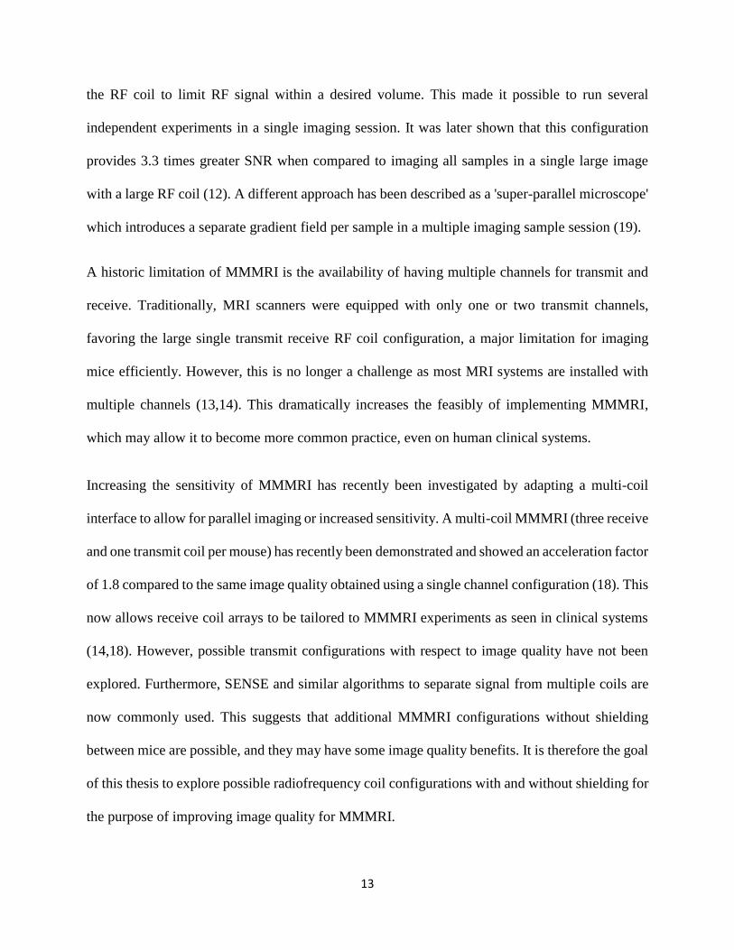
SNR results show that our three loop design resulted in the highest SNR (figure 8). Figure 8 shows
normalized SNR (normalized to the three loop coil) as a function of calculated coil inductance. As
expected, the increase in B1 magnitude resulted in an increase in SNR. Overall a 77% increase in
SNR was seen between a single loop 120 degrees aperture and a three loop coil. In addition, a large
B1 Line Profile Across X Axis
-30 -25 -20 -15-10 -5 0 5 10 15 20 25 30-1.0
-0.5
0.0
0.5
1.0 120 Deg
180 deg
2 Loop
2 Loop Parallel
3 Loop
4 Loop
X Position (mm)
No
rmalized
B1
X
Z
A
B
19
increase of 50% was seen between the 120 and 180 degrees aperture with only a smaller difference
between the 2 and 3 loops coils (33%). This suggests that adding more loops (or increasing coil
inductance) at this point offers diminishing SNR returns. This indicates a relationship where the
sensitivity (ability to acquire signal) of adding more loops is offset by the addition of more coil
resistance, a result not unexpected for high fields. In addition, adding more inner loops, (with
progressively smaller diameter) will cause these loops to have smaller sensitive regions, reducing
the benefit through much of the coil.
Figure 8: The three loop saddle coil provided the highest SNR when compared with four other feasible
configurations. Normalized SNR as a function of coil inductance (nH). The joining curve connects all coils
connected in series (circles) while the square point represents the parallel connection saddle.
In all cases Lf values remained the same at around 0.5±0.05. This suggests that coil and sample
noise contribute about equally in all cases. Therefore, when adding more loops, the relative sum
of coil and sample noise may be reduced if coil noise increases less, providing a higher SNR in
the image.
With the support of this data, we concluded that a three loop saddle coil would be appropriate for
in vivo mouse brain imaging. Construction of these coils is difficult, and in order to maintain
Rx Coil Inductance
0 200 400 600 8000.0
0.2
0.4
0.6
0.8
1.0
1 Loop 120 deg
1 Loop 180deg
2 Loops
3 Loops
2 Loops Parallel
Coil Inductance (nH)
No
rmalized
SN
R

20
consistency and to be able to create many of them for MMMRI a form was designed (courtesy of
Jun Dazai) for the three loop saddle coil (Fig. 9). Coils for the remainder of this thesis were
constructed using this form.
Figure 9: Final three loop saddle coil design using a custom form. This coil is used throughout thesis. A: A
Computed-aided design (CAD) drawing of a three loop saddle coil (courtesy of Jun Dazai). Loop wires are
positioned one diameter apart to minimize capacitive and proximity effects. B: Photo of actual three loop saddle coil
in a clear form showing segmenting capacitors.
2.2 MMMRI Configurations
To compare possible Tx and Rx coil configurations four cases were tested using the simple case
of two samples placed 60mm apart. I compared four configurations, shown in figure 10. Briefly,
Case A is composed of a shielded Tx coil surrounding individual Rx saddle coils. In case B, saddle
coils operate in a transmit-receive mode surrounded by a copper shield. In case C, one single large
Tx coil encompasses all individual saddle Rx coils. In case D, saddle coils operate in a transmit-
receive mode without any shields. I used SNR measurements to compare these configurations.

21
2.2.1 Methods
Phantom based SNR measurements were taken with 10mL 1% agar phantoms electrically loaded
with 0.9% saline to simulate a mouse's head. In Case A, (Fig. 10A) two shielded birdcage Tx coils
(outer diameter [OD] 60mm, inner diameter [ID] 40mm, RAPID MR International) were mounted
adjacent to one another, with two three loop saddle coils (ID 19mm) to serve as Rx coils. In this
configuration, only Tx-Rx interactions must be considered and not Rx-Rx interactions due to
shielding of the Tx coils. Therefore Tx and Rx coils were placed so that their fields are orthogonal
to each other (geometrically decoupled) to avoid any coupling effects. This approach is similar to
the method used in Bock et al (8), where each mouse is isolated from one another and allows us to
conduct isolated experiments. Case B, (Fig. 10B) consisted of the three loop saddle coils operating
in a transmit-receive (Tx-Rx) mode with a 60mm diameter copper shield surrounding each coil.
This case provides similar benefits to Case A however no coil-to-coil interactions need to be
considered. Case C, (Fig. 10C) involved a single large-volume shielded birdcage Tx coil (OD
154mm, ID 135mm, RAPID MR International) of sufficient size to image at least 7 mice
simultaneously, surrounded by unshielded three loop saddle Rx coils (positioned in the same
orientation). Once again, the large Tx coil and Rx coils with positioned orthogonally to one another
to prevent any coupling between the two. In addition to the Tx-Rx interactions described above,
this configuration must also consider Rx-Rx interactions. Here, the ability to run separate
independent experiments is lost. For example, using separate transmit frequencies per sample is
not possible. Case D, (Fig. 10D) consisted of two adjacent three loop saddle coils in the same
orientation operating in a Tx-Rx mode without any shielding. Here, Rx-Rx interactions must be
considered, as described above, and Tx-Tx interactions are also possible. Large field of view
(LFOV) images were acquired in all cases using a gradient echo sequence with a field of view
(FOV) encompassing all samples, with the following parameters: (TR=50ms, TE=4.55ms,

22
Matrix:128[readout]x704[phase encoding] FOV:5.12x14.1cm, flip angle=90degrees, number of
averages= 2, slice thickness= 3mm and scan time = 1 minute 10 seconds). LFOV images
eliminated the need to further post process images using a SENSE algorithm, enabling assessment
of each configuration based on SNR.
Figure 10: Four RF coil configurations tested for MMMRI. A: Two shielded birdcage Tx coils mounted next to one
another with saddle coils as Rx. B: Two saddles coils operating in a Tx-Rx mode with 60mm diameter shield
surrounding them. C: One large Tx birdcage coil surrounding two Rx saddle coils. D: Two exposed saddle coils
operating in a Tx-Rx mode. B1 generating by the saddle coils and birdcage coils are shown in red and blue
respectively, indicating that coils are geometrically decoupled.
2.2.2 Results
The RF coil configuration experiment showed two distinct pairings based on the effect of shielding
(figure 11). Here the average of three measurements is plotted against normalized SNR (with
standard deviations). First, cases A and B both represent individually shielded experiments and
have a normalized average SNR of 83±6% and 80±8% respectively. Second, case C and D both

23
eliminate shielding effects however introduce Rx-Rx interactions and have a normalized SNR of
100±4% and 93±2%, respectively.
Figure 11: RF configuration tests in an agar phantom indicate that either a large single Tx coil or RF coils in a Tx-
Rx mode without shielding provided the highest SNR. Values are normalized to the average of the large single Tx
coil. Errors bars indicate the standard deviation of three measurements.
2.3 The Effect of Shielding Results from above indicate that shield effects may degrade image quality by up to 20%. To further
understand coil-to-shield interactions, a further experiment was conducted using our three loop
saddle coil in a Tx-Rx mode with the same phantoms described above. This shielding effect is very
likely to have a geometry dependence, therefore shields of varying diameter were tested.
SNR of Different RF Coil Configurations
A, I
ndivid
ual T
x
B, T
R w
ith S
hield
ing
C, L
arge
Sin
gle T
x
D, T
R N
o Shie
ldin
g
0.0
0.5
0.6
0.8
1.0
RF Coil Configuration
No
rmalized
SN
R

24
2.3.1 Methods
In this experiment images were acquired using a two-dimensional gradient echo sequence with
parameters: TR=50ms, TE=4.55ms, Matrix:512x512 FOV:5.12x5.12cm, flip angle= 90 degrees,
slice thickness= 3mm, number of averages= 2 and scan time = 50 seconds. The shield diameters
that were tested were: 45mm, 60mm, 75mm, 120mm and 290mm (diameter of our gradient bore).
Three different coils were tested with all shields and SNR measured.
2.3.1 Results
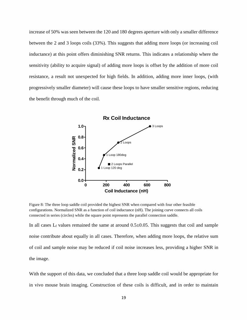
Normalized SNR was found to be directly related to the shield diameter (Figure 12, slope = -0.94
and R2=0.92). These results are consistent with the empirical relationship in equation 13, where
this line should have slope of -1. Equation 13 indicates that the effect of shield on a coil is geometry
dependant (38). The bigger the shield, the better the coil performance. A total measured loss of
15% was seen in decreasing the shield diameter from 290mm (gradient bore diameter) to 60mm
(diameter of shield and Tx coil used in figure 11). This suggests that the 20% difference in SNR
seen between our cases (A,B and C,D) is due to the effect of shielding.
25
𝑁𝑜𝑟𝑚𝑎𝑙𝑖𝑧𝑒𝑑𝑆𝑁𝑅 = 1 −𝐶𝑜𝑖𝑙 𝐷𝑖𝑎𝑚𝑒𝑡𝑒𝑟
𝑆ℎ𝑖𝑒𝑙𝑑 𝐷𝑖𝑎𝑚𝑒𝑡𝑒𝑟 [13]
Figure 12: Shielding of RF coils lowers SNR, this difference of SNR accounts for the variation in SNR in figure 13
(configurations A,B versus C,D ). Inverse shield diameter (1/mm) is plotted against normalized SNR. The red
continuous line represents a regression line with 95% confidence interval (dash curve) to compare results to the
expected relationship in equation 13.
The results from this section and the previous section favor a mouse array of a single large Tx coil
encompassing all mice with individual Rx coils (Case C), or of saddle coils in a Tx-Rx mode
without any shields (case D). We will favour case C, due to its simplicity, since case D would
required additional electronics to ensure that Tx-Rx interactions are eliminated in a MMMRI array,
which can reduce SNR by up to 10% (21). In case C, both Tx-Rx and Rx-Rx interactions must be
minimized, through mutual inductance.
2.4 Receive Geometries and Coupling
Induced B1-field is dependent on the rotation of our saddle coil, therefore coupling can be reduced
by coil separation and coil orientation. This can be accomplished either by rotating or separating
adjacent coils. Three more experiments were conducted: i) rotating two coils at a fixed separation,
Shielding of Radiofrequency Coils
0.000 0.005 0.010 0.015 0.020 0.0250.0
0.5
0.7
0.8
0.9
1.0
1.1
1/Shield Diameter (mm)
No
rma
lize
d S
NR

26
ii) changing the distance between coils with two fixed rotations and iii) shifting the coils along Lo
(figure 6, the B0 or z direction) at a fixed rotation. It is well known that placing linear coils
orthogonal to one another will eliminate inductive coupling between the two. However, in a
multiple mouse array, not all coils can be placed orthogonal to one another and many interactions
can take place. Therefore, other possible configurations must be investigated.
2.4.1 Rotation
In this experiment two three loop saddle coils were placed adjacent to one another at a fixed centre-
to-centre distance apart of 60mm. By using symmetry only a select number of orientations were
tested (Table 1), these included: 0-0, 0-30, 0-60, 0-90, 30-30, 30-60, 30-90, 60-60,60-90 and 90-
90 degrees. Each orientation was measured as the counter clockwise rotation from the 0 degrees
orientation, where the induced B1-field in the saddle coil is vertical. Images were then acquired
using a two dimensional gradient echo (TR=50ms, TE=4.55ms, Matrix:256x704
FOV:5.12x14.1cm, flip angle= 90 degrees, number of acquisitions= 2, slice thickness= 3mm and
scan time = 1 minute 10 seconds). This experiment was repeated using three combinations of three
different saddle coils. Once again large FOV images were acquired so that no post processing was
necessary. We used the same calculation in section 2.1.1 to predict the mutual inductance between
two coils. Mutual inductances were calculated with both coils rotated from zero to 90 degrees and
plotted on a contour plot (figure 13B).

27
Table 1: Orientation (in degrees) of adjacent saddle coils for Rx coil rotation test
Coil Degree 0 30 60 90
0
30 -
60 - -
90 - - -
Figure 13: The relative orientation of two adjacent saddle coils causes changes in mutual inductance that were found
to significantly affect image quality. A. SNR using 10 different orientations of two Rx coils. The error bars
represent standard deviation values of three measurements. B. A contour plot of calculated mutual inductance
between two coils with varying degrees of rotation.
The ideal rotation was found to be 0-90 degrees with a 25% increase in SNR relative to the poorest
rotation of 90-90 (figure 13). For the most part, expected trends (calculated in Figure 13B) are
seen. For example, an increase in SNR is seen from coils approaching the ideal 0-90 degrees
orientation and away from the non-ideal 90-90 degrees orientation. The 30-30 and 30-60
orientations did not perform as well as expected, which may imply coupling through means other
than mutual inductance.
Rx Coil Rotation
0-0
0-30
0-60
0-90
30-3
0
30-6
0
30-9
0
60-6
0
60-9
0
90-9
0
0
700800
900
1000
1100
1200
1300
Rotation (Degrees)
SN
R
A B

28
2.4.2 Translation
Our next experiment tested how significantly the perpendicular distance between coils affected
image quality. Two three loops saddle coils were oriented in a 0-0 degrees position and the
separation between the two coils was tested at 40mm, 50mm, 60mm and 70mm. Images were
acquired using a two dimensional gradient echo (TR=50ms, TE=4.55ms, Matrix:128x704
FOV:5.12x14.1cm, flip angle= 90 degrees, number of acquisitions= 2, slice thickness= 3mm and
scan time = 1 minute 10 seconds). Again three combinations using three different saddle coils were
used and LFOV images acquired. This experiment was then repeated in a 0-90 degrees orientation
to further characterize the interaction. A similar calculation of mutual inductance to the one
described above was also conducted at fixed rotations and by varying the centre-to-centre coil
translations. These results are plotted in figure 14B.

29
Figure 14: Changing the centre-to-centre distance between coils increases SNR while the mutual inductance is
decreased. A. SNR with centre-to-centre distance of two Rx saddle coils at 0-0 degrees (black) and 0-90 degrees
(red). The error bars represent standard deviation values of three measurements. B. Calculated mutual inductance
values between two coils at 0-0 degrees (black line) and 0-90 degrees (red line).
As the distance increases between the two adjacent coils, the mutual inductance and coupling
between them decreases (figure 14). In the first of these experiments the coils were placed in a 0-
0 degrees orientation where mutual inductance is more significant. We observed the expected trend
of decreased inductance and higher SNR. A 25% difference in SNR was seen between 40 and
Translation of Rx Coils
30 40 50 60 70 800
500600
800
1000
1200
1400
0 0 Degrees
0 90 Degrees
Distance Apart (mm)
SN
R
Mutual Inductance Between 2 Saddle Coils
30 40 50 60 70 800
5
10
15
20
250-0 Deg
0-90 Deg
Centre-to-Centre Distance (mm)
Mu
tual In
du
cta
nce (
nH
)
A
B

30
70mm separation. When the pair of coils was placed orthogonal to one another, the mutual
inductance was minimized and a 16% difference in SNR was seen between coils 40 and 70 mm
apart.
2.4.3 Depth
Our final experiment tested how shifting the coils along Lo (figure 6, the B0 or z direction) affected
mutual inductance and SNR. Two three loops saddle coils were oriented at 0 degree (0-0 pair) and
with a centre-to-centre separation of 60mm. One coil was adjusted and moved with respect to Z at
centre-to-centre distances of 0mm, ±20mm, ±40mm, and ±60mm. Images were acquired with the
following parameters: TR=50ms, TE=4.55ms, Matrix:128x704 FOV:5.12x14.1cm, flip angle= 90
degrees, number of acquisitions= 2, slice thickness= 3mm and scan time = 1 minute 10 seconds.
Afterwards a mutual inductance calculation was conducted using the method described above.
These results are plotted in figure 15.

31
Figure 15: Another method to reduce coupling and increase SNR is by shifting the coils along Lo (the z axis). A.
SNR depth results using two Rx coil rotation 0-0 degrees. The error bars represent standard deviation values of
three measurements. B. Calculated mutual inductance values between two coils of different depths.
As the Lo separation increases between the two adjacent coils, the mutual inductance and coupling
between them decreases. Here a 29% decrease in SNR was seen at 0mm compared to ±60 mm.
The results also demonstrate the expected results of symmetry about 0mm.
Rx Coil Shift
-100 -50 0 50 1000
800900
1000
1100
1200
1300
1400
Centre-to-Centre Distance (mm)
SN
R
Mutual Inductance Between 2 Saddle Coils
-100 -50 0 50 1000
1
2
3
4
Z Distance (mm)
Mu
tual In
du
cta
nce (
nH
)
A
B

32
2.4.4 Coupling and SNR
The above experiments confirm that mutual inductance between two coils affects image quality.
This section aims to quantify this relationship more generally. This is achieved through a simple
circuit model (figure 1) which states that mutual inductance will increase the coil impedance, thus
decreasing image SNR.
2.4.4.1 Methods
A simple model expresses SNR as a function of: (i) both coil and sample resistance (R1) and (ii)
the coupling of resistance from adjacent coils (R2) by mutual inductance, equation 14. Thus it can
be shown without any coil coupling (zero mutual inductance) the expected value of only coil
resistance is achieved. Using a multi meter, coil resistance was measured to be one ohm, and
assuming a loading factor of 0.5, sample resistance should also be one Ohm. This yields a total
resistance in each coil of two Ohms. In our model, mutual inductance allows for additional
resistance to be introduced within the coil and thus lower image quality. This can be calculated
using a LRC model of two adjacent three loop saddle coils, as expressed in equation 14:
𝑆𝑁𝑅 𝛼 1
√𝑅1+𝜔2𝑀2
𝑅2
[14]
It is important to indicate that the calculated value from equation 14 only accounts for mutual
inductance between the coils and that capacitive coupling between coils may also occur.
2.4.4.2 Results
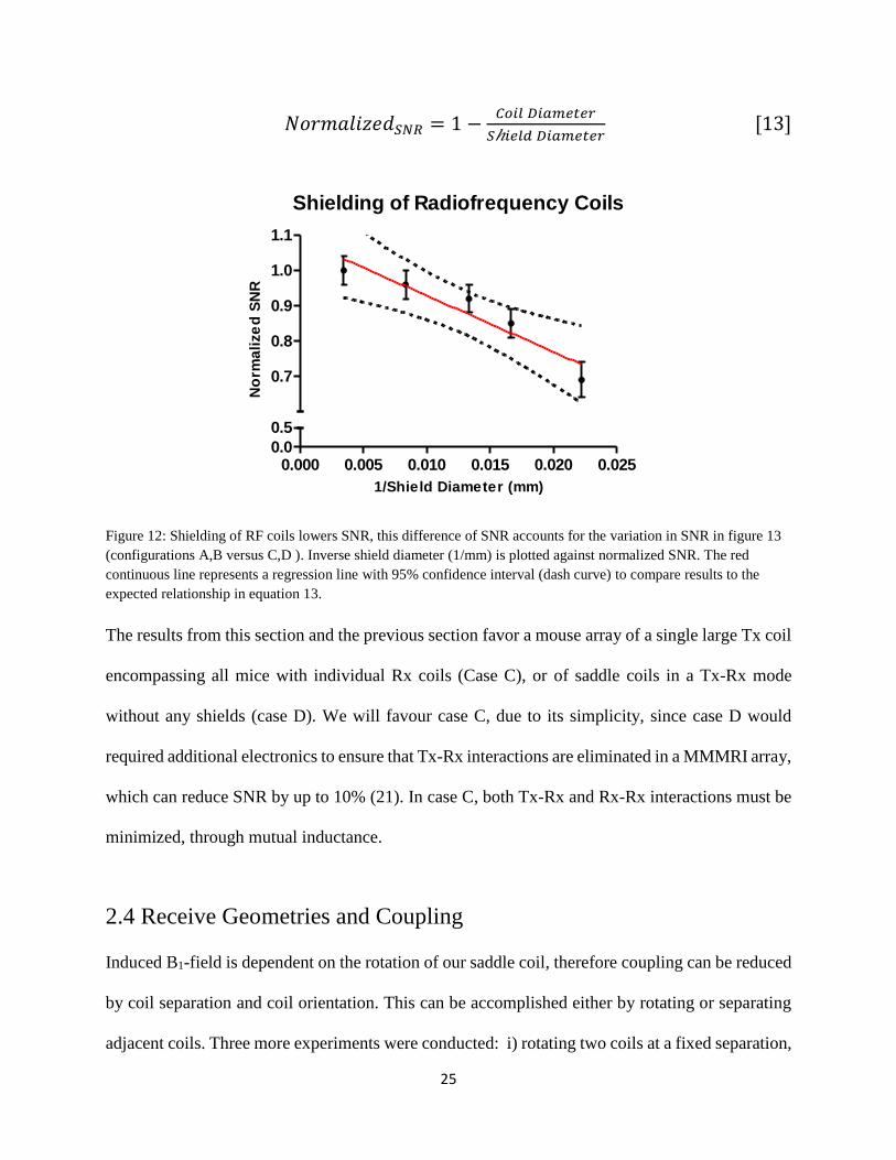
Figure 16, 1/ normalized SNR2 is plotted as a function of mutual inductance squared (M2) shown
in equation 14, which should provide a linear relationship. The solid line in the figure represents a
linear regression with 95% confidence intervals shown.
33
Mutual Inductance and SNR Between 2 Saddle Coils
0 20 40 60 80 1000.0
0.5
1.0
1.5
2.0
M2(nH
2)
1/S
NR
2(x
10
-6)
Figure 16: Modeling SNR from M indicates that image quality is decreased due to the addition of impedance from
adjacent coils. 1/SNR2 as a function of predicted mutual inductance squared. This figure contains the results of all
data in 2.4.1, 2.4.2 and 2.4.3. The black line is a linear regression with 95% confidence interval. Colour points
represent rotations: 0-0 red, 60-60 green, 90-90 yellow and 30-60 purple.
Qualitatively, the linear relationship from equation 14 holds. As mutual inductance increases, extra
impedance from the adjacent coil is added and lowers SNR. However, the variance around the fit
line is somewhat high, likely due to other types of coupling, i.e. capacitive coupling. For example,
within the rotation result values (0-0 red, 60-60 green, 90-90 yellow and 30-60 purple), coils are
positioned in a parallel orientation to one another, meaning the rungs along the saddle are all in
the same direction and at the closest possible distance to one another. This may provide increased
capacitive interactions and thus result in a lower SNR than expected. Also, points within the circled
region all have very low mutual inductances and fall below (larger SNR than expected) the 95%
confidence interval. These positions have very low mutual inductances, so that coupling by other
means may dominate SNR outcome.
Despite the possibility of other effects, figure 16 shows that mutual inductance is an important
factor in coupling coils, resulting in a decreased image SNR. This is an important consideration

34
when designing an array to image multiple mice simultaneously, especially if coils are unshielded
and operating in a Tx-Rx mode. Figure 16 suggests that minimization of mutual inductance during
array design provides a means of optimizing the expected SNR. Note that it is likely that a SENSE
reconstruction, which was not used in Figures 13 through 16, can recover some of this SNR and
decrease the SNR dependence on mutual inductance. However, this benefit of SENSE
reconstruction—and indeed SENSE reconstruction in general—is dependent on orthogonal coil
sensitivities, a property also degraded by coil coupling by mutual inductance or other means.
Hence, the degree to which SNR can be recovered is fundamentally limited, and minimization of
mutual inductance (and any other means of coupling) is an important consideration for multiple-
mouse coil arrays.
Array design with respect to coils must consider two dimensions; orientation and distance apart.
With respect to coil rotation, our model of computed SNR as a function of mutual inductance
(figure 16) can be used to determine the ideal coil rotation. In addition, the distance apart must be
kept as large as possible to minimize inductance (and capacitive) coupling to keep image quality
high. Additional factors to take into consideration include the number of mice, bore diameter and
animal handling.
2.5 Theoretical Design of a MMMRI Array
A total of seven mice was chosen to be imaged at once. This number is convenient geometrically
in the dimensions of our gradient bore. The most efficient method to position seven mice within a
bore of 210mm in diameter is to have three rows of mice, with two on the first row (top), three on
the second (middle) row and two on the third (bottom) role. In this configuration the maximum
distance apart is 60mm. However, to accommodate an existing rail system that allows efficient

35
placement of coils and mice in the bore, a centre-to-centre separation distance of 58mm was
chosen. In addition, different depth positions can be considered for possible array configurations.
To determine which orientations are ideal in a seven coil array that minimize the mutual
inductance, we computed all pair wise mutual inductances in the array as seen in section 2.4.
Within a seven coil array system there will be six pairs of nearest coil interactions (adjacent coils
separated by 58mm) and 15 pairs of second order interactions (coils separated by more than
58mm). Here, all 21 mutual inductance pairs functions were used as inputs in a nonlinear least
squares minimization (the Levenberg-Marquardt algorithm) (39) with all 7 coil rotations and z
positions as independent variables. Shown in equation 15:
min𝑥,𝑧
‖𝑓(𝑥)‖22 = 𝑚𝑖𝑛𝑥1−7,𝑧1−7
∑ ∑ 𝑓2(𝑥𝑖 , 𝑥𝑗 , 𝑧𝑖 , 𝑧𝑗)𝑁𝑗=𝑖+1
𝑁−1𝑖=1 [15]
Here each function f represents the mutual inductance of a pair of coils where x is the rotation of
each coil, z the depth position and i,j index the coils for a total of 21 pairs. The sum of all 21 pairs
of mutual inductance squared was then minimized. To ensure we remain within the gradient
volume, a maximum z distance between any two coils was set to be 50mm. Several starting
positions were chosen at random, all of which resulted in similar orientations with symmetric
properties. Shown in figure 17 is the orientation that minimized all 21 local pairs. There is a
consistent symmetry in all the solutions from random start points (figure 17).
36
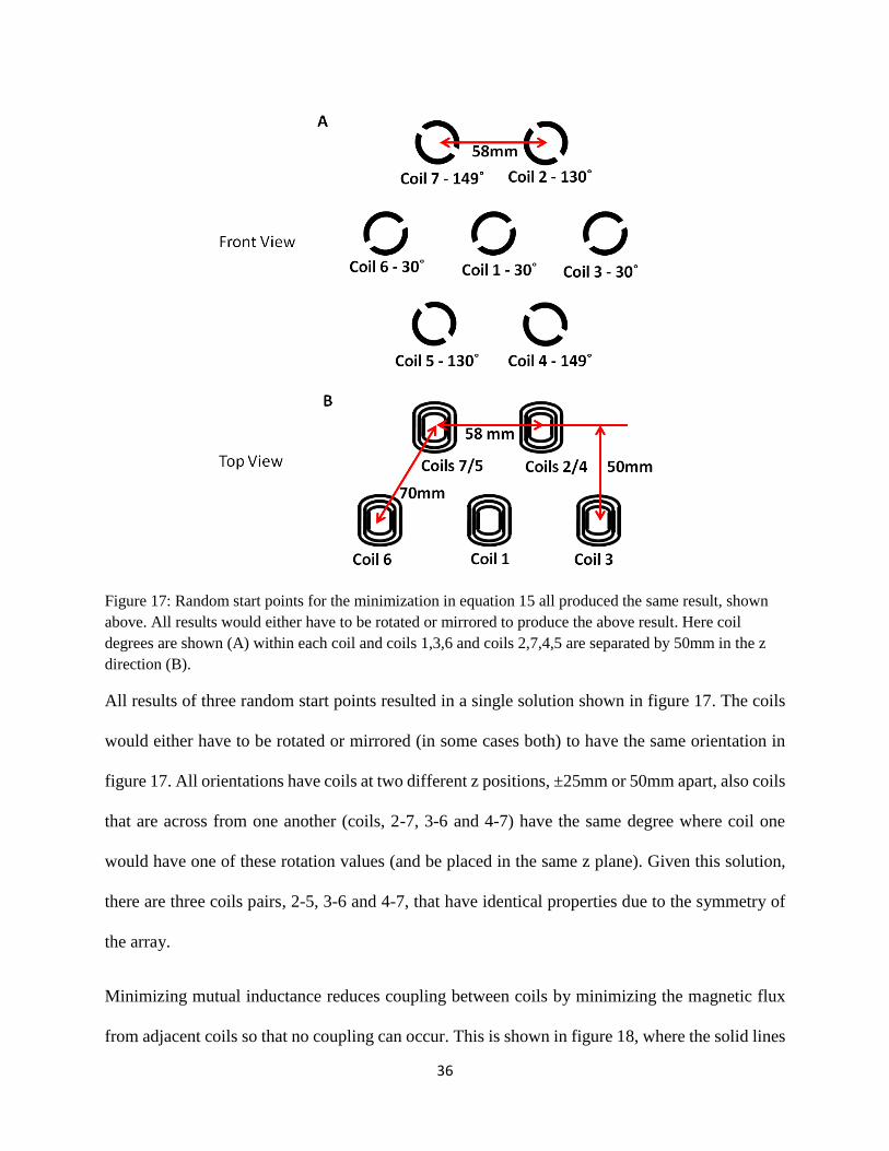
Figure 17: Random start points for the minimization in equation 15 all produced the same result, shown
above. All results would either have to be rotated or mirrored to produce the above result. Here coil
degrees are shown (A) within each coil and coils 1,3,6 and coils 2,7,4,5 are separated by 50mm in the z
direction (B).
All results of three random start points resulted in a single solution shown in figure 17. The coils
would either have to be rotated or mirrored (in some cases both) to have the same orientation in
figure 17. All orientations have coils at two different z positions, ±25mm or 50mm apart, also coils
that are across from one another (coils, 2-7, 3-6 and 4-7) have the same degree where coil one
would have one of these rotation values (and be placed in the same z plane). Given this solution,
there are three coils pairs, 2-5, 3-6 and 4-7, that have identical properties due to the symmetry of
the array.
Minimizing mutual inductance reduces coupling between coils by minimizing the magnetic flux
from adjacent coils so that no coupling can occur. This is shown in figure 18, where the solid lines

37
represent the general direction of the magnetic field produced in coils one through four. Here the
magnetic field produced by a certain coil offers an almost perpendicular orientation to adjacent
coils, decreasing the flux and therefore mutual inductance.
Figure 18: Coils are orientated such that the produced B1 field (red) crosses adjacent coils at nearly an orthogonal
orientation, thus reducing flux and coupling. These B1 field maps represent the final orientation of coils 1-4 (A-D).
Coils that are positioned within the same plane are coloured the same (1-3-6 and 2-4-5-7). B1from coil 5,6 and 7 (not
shown) have the same results as coils 2,3 and 4 respectively due to symmetry of the array.
The question of how sensitive the minimization is to coil orientation could be quite important in
the design of a MMMRI array, for two reasons: i) it determines tolerance on coil orientation in
array construction and assembly and ii) array usage could permit unintentional coil orientation
shifts. To predict tolerance, total mutual inductance (the sum of all 21 pairs squared) was calculated
for ±30 degrees for all coils from the orientation in figure 17. Results are shown in figure 19. These
results show that all coils are quite stable and have a ±10 degrees tolerance for 0.5 nH of extra

38
total mutual inductance. Therefore we can conclude that our reference position is at a favoured
position and is quite stable. We now have an orientation where all seven coils in the array receive
equally low mutual inductance values and are stable with respect to their orientation of ±10
degrees.
Coil Orientation Sensitivity
-40 -20 0 20 400
1
2
3
4Coil 1
Coil 2
Coil 3
Coil 4
Degree Change
To
tal M
utu
al In
du
cta
nce (
nH
)
Figure 19: Total mutual inductance as a function of degree change of all four coils in our final orientation. Coil
orientations are shown to be robust as ±10 degree change from figure 17 only adding 0.5nH of total M. Coils 2,3,4
are identical with coils 5,6 and 7 (not shown) respectively due to the symmetry of the array.
Next we designed an array for MMMRI. In this component I worked closely with Jun Dazai, a
mechanical engineer at the Mouse Imaging Centre. The array was designed using the CAD
software Autodesk Inventor (San Rafael, California, U.S) and incorporated all necessary
components for live mouse imaging. These include: anesthesia gas delivery, gas scavenging,
temperature monitoring, respiratory monitoring, heat delivery and proper holding for the mouse.
A fully labelled CAD image is shown in figure 20A (courtesy of Jun Dazai) accompanied by a
photo (B). Each coil contains its own tooth bar, where the mouse is held securely in place and
anesthesia delivered. The coil form itself acts to contain the anesthesia so that efficient scavenging

39
can occur, this feeds onto a main manifold where scavenging is achieved through one of the four
outer rods. Respiratory and temperature monitoring lines are fed through each individual mouse's
line. The mouse's body sits in a semi-circular exposed tube that permits imaging of both small and
large mice. Heat is provided through hot air delivered through the bottom two outer rods. All coils
matching circuits are shielded from one another using copper foil to avoid any unnecessary cross
talk. Finally the array is held secured in the magnet bore via a pneumatic compressed air clamp.
The array was constructed using a CNC milling machine with non-magnetic components. Coils
were rotated and positioned to the orientation shown in figure 17.
Figure 20: A. A labelled CAD drawing of a seven multiple mouse live head imaging array, courtesy of Jun Dazai.
The array includes seven three loop saddle RF coil for imaging, semi circular mouse bed to accommodate large
mice, individual anesthesia, scavenging and monitoring per mouse and global heat delivery. B. Photo of the array
with the two lower beds connected and all lines and coils shown.
2.6 Imaging with the array
Once the array was constructed initial tests were completed in phantoms. This was to ensure our
SENSE-like reconstruction was sufficient to eliminate ghosts and to observe any trade off in image

40
quality when having seven coils in an array. Afterwards high resolution live images were acquired
using seven mice and images reconstructed using our SENSE-like method.
2.6.1 Methods
To demonstrate that the SENSE algorithm could eliminate ghosting, phantoms images where
acquired using a cylindrical gradient echo sequence. A cylindrical k-space acquisition, where the
corners of k-space are not acquired in 2 dimensions, was used to save time (40). The cylindrical
acquisition allows us to image in ~28% less time than a standard acquisition. A low resolution
large FOV image that encompassed the entire range to capture all seven phantoms was also
acquired (T1 weighted, TR=60ms, TE=6.05ms, Matrix:388x75x75 FOV:3.5x13.5x13.5cm, flip
angle= 45 degrees, number of acquisitions=1, scan time= 4 minutes 33 seconds). This image was
used to calculate our sensitivity matrix, which was used to eliminate ghosts in our desired high
resolution small field of view (SFOV) images (T1 weighted, TR=60ms, TE=6.05ms,
Matrix:388x222x278 FOV:3.5x2.0x2.5cm, flip angle= 45 degrees, number of acquisitions= 3,
scan time = 2 hour 28 minutes). Once the LFOV images were acquired a 7x7 sensitivity matrix
was created. This matrix contains cross talk coefficients, from each coil to every other coil (with
diagonal entries equal to unity). This matrix was computed using the large FOV data, where for
each coil each ghost average intensity value was divided by its own average intensity value, much
like a normalization. This was completed for both the magnitude and phase (complex conjugate)
of the data. This provided our sensitivity matrix or C values in equation 9.
Live mouse imaging were acquired using the same two sequences describes above. 24 hours before
imaging mice were injected with a manganese chloride solution (0.4 mmol/kg) to provide the
desired contrast. The mice were anesthetized using 2% isoflurane, maintained at 1-1.5%
isoflurane, and kept at a constant temperature of 29 degrees Celsius. All animal experiments were
41
approved by the Animal Care Committee at the Toronto Centre for Phenogenomics (animal use
protocol 0227).
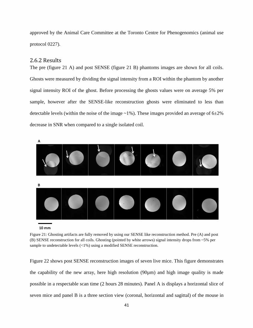
2.6.2 Results The pre (figure 21 A) and post SENSE (figure 21 B) phantoms images are shown for all coils.
Ghosts were measured by dividing the signal intensity from a ROI within the phantom by another
signal intensity ROI of the ghost. Before processing the ghosts values were on average 5% per
sample, however after the SENSE-like reconstruction ghosts were eliminated to less than
detectable levels (within the noise of the image ~1%). These images provided an average of 6±2%
decrease in SNR when compared to a single isolated coil.
Figure 21: Ghosting artifacts are fully removed by using our SENSE like reconstruction method. Pre (A) and post
(B) SENSE reconstruction for all coils. Ghosting (pointed by white arrows) signal intensity drops from ~5% per
sample to undetectable levels (<1%) using a modified SENSE reconstruction.
Figure 22 shows post SENSE reconstruction images of seven live mice. This figure demonstrates
the capability of the new array, here high resolution (90µm) and high image quality is made
possible in a respectable scan time (2 hours 28 minutes). Panel A is displays a horizontal slice of
seven mice and panel B is a three section view (coronal, horizontal and sagittal) of the mouse in
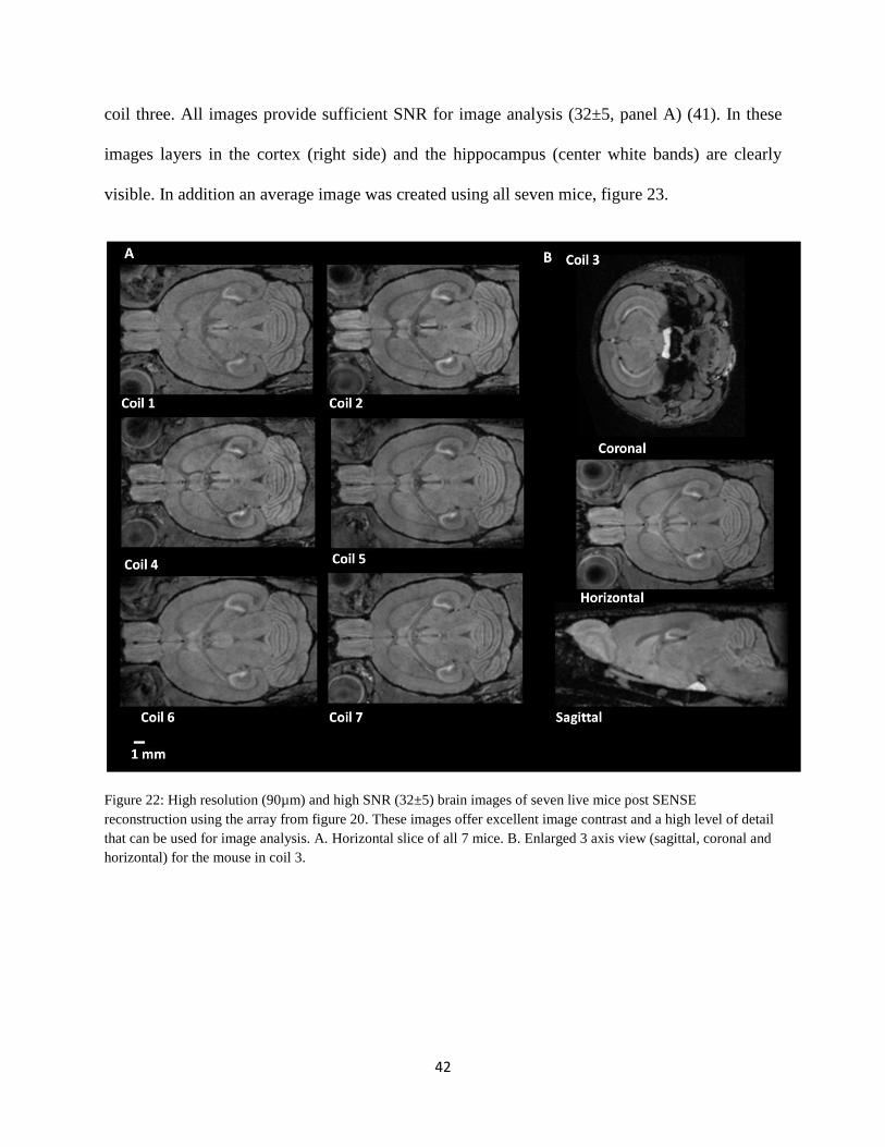
42
coil three. All images provide sufficient SNR for image analysis (32±5, panel A) (41). In these
images layers in the cortex (right side) and the hippocampus (center white bands) are clearly
visible. In addition an average image was created using all seven mice, figure 23.
Figure 22: High resolution (90µm) and high SNR (32±5) brain images of seven live mice post SENSE
reconstruction using the array from figure 20. These images offer excellent image contrast and a high level of detail
that can be used for image analysis. A. Horizontal slice of all 7 mice. B. Enlarged 3 axis view (sagittal, coronal and
horizontal) for the mouse in coil 3.

43
Figure 23: Three dimensional average image of all seven mice from figure 22. Coronal (top), horizontal (middle)
and sagittal (bottom). This average can be used as a template for image analysis for future experiments.

44
Chapter 3
MMMRI Coil Array
3.1 Benefits My investigation of RF coil configurations for live mouse brain imaging resulted in the design of
a MMMRI array with three loop saddle coils operating in a Tx-Rx mode. Even without shields and
when operating in a seven coil array, coil coupling could be minimized using geometry of coil
placement and then corrected using a SENSE-like reconstruction. One can trade off this added
benefit, according to the relationship:
𝑆𝑁𝑅 ∝ ∆𝑥∆𝑦∆𝑧√𝑁𝑎𝑣𝑔𝑁𝑝𝑒 [16]
One can i) increase resolution (by decreasing Δx, Δy and Δz) and/or ii) decrease scan time (reduce
number of averages, Navg or number of phase encoding steps, Npe). For example, given equation
16, a 50% increase in SNR will provide a 17% increase in resolution for an isotropic 3D image.
Live mouse imaging is typically SNR limited and there is a limited time a mouse could be
anesthetized, scan time for mice must be limited to ~3 hours. Therefore, resolution is often
sacrificed in order to acquire sufficient signal. When resolution is sufficient, the increased SNR
provided by this array can benefit many imaging protocols. For example, functional MRI uses
blood oxygen level dependant (BOLD) signal and depends on the detection of small signal changes
(a few percent). Having higher SNR results in higher sensitivity to the BOLD effect.
Some longitudinal studies may now be more feasible. This involves increasing resolution while
decreasing scan time. The high resolution capability of sensitive coils will make it possible to
image young mice and still be able to detect brain differences. Here the increased coil sensitivity
may be traded for shorter scans (25% shorter), allowing more frequent scanning sessions to occur.
45
For example, a young mouse could be imaged at post natal day 14 with subsequent imaging every
two to three days afterwards to track more rapid changes in early development. I anticipate that
this is one of the greatest benefit of the new saddle-coil array for mouse imaging.
3.2 Potential Use
Interest in 3D imaging in biology has increased throughout the past 10 years. However, standard
imaging modalities based on histological techniques and microscopy are cumbersome to adapt to
3D. Three-dimensional MRI minimizes distortion artifacts produced during fixation, embedding,
sectioning and mounting for histological methods. MRI also provides excellent soft tissue contrast
and the ability to perform in vivo experiments.
My seven coil live mouse imaging array provides high throughput and high quality images and
could be implemented in any laboratories that already have access to a modern MRI scanner. The
RF design and matching circuit can easily be constructed and do not require expensive
components. Labs inexperienced with multiple-mouse MRI may encounter three difficulties
associated with implementation of the seven coil array: i) Instrumentation, ii) Construction and iii)
Image reconstruction. With respect to instrumentation, current clinical MRI scanners are being
equipped with multiple Tx and Rx channels to allow for more efficient human imaging. In many
cases, a scanner will have up to 16 Tx and 32 Rx channels, therefore up to 16 samples could be
imaged in a Tx-Rx mode for multiple specimens. In addition, clinical scanners already have large
bore sizes that would provide enough room for a multiple sample array. However two limiting
factors of clinical systems are their magnetic field strength and gradient strength. The lower field
strength of clinical systems results in a lower SNR whereas a smaller gradient strength would limit
image resolution. The saddle design would promote high sensitivity to overcome low field

46
strength, however gradient strength may still limit resolution. Overall, however, modern MRI
systems are equipped with the instrumentation required to operate the multiple-mouse coil array
designed in this thesis. Construction of the array is an issue for labs that do not have their own mill
nor CAD software. However, this could potentially be outsourced for a relatively low cost. As
shown in my second chapter, coils should be placed as far apart as possible given the number of
coils and gradient boundaries. Coil rotation can be determined using the mutual inductance least
square minimization method. This will ensure that coupling is at a minimum and image quality
high. Finally image reconstruction will be achieved using a SENSE-like method. Clinical systems
do come equipped with standard SENSE methods, where my method could easily be adapted;
since coil sensitivities are kept constant over an image, ghosts can be easily removed via a simple
subtraction.
3.3 Custom Coils
This thesis introduces an idea that has been practised in clinical systems over the past few years.
That is, custom coils or arrays tailored to a specific applications or imaging protocols. In this thesis,
a custom coil was designed for live mouse head imaging. After a coil was designed and built, a
multiple mouse imaging array was constructed. Generic systems with large volume coils have the
potential to suffer in two ways, i) image quality and ii) imaging efficiency (handling and
throughput). Creating custom coils and/or arrays solves these issues. During my time at the Mouse
Imaging Centre, an investigation was completed where a custom set up was needed and
constructed for intubated mice for arterial spin labeling (ASL) and cerebral blood volume (CBV)
measurements. Projects were completed with Dr. Cahill from the Mouse Imaging Centre and
apparatus design and construction was completed by our mechanical engineer Jun Dazai.
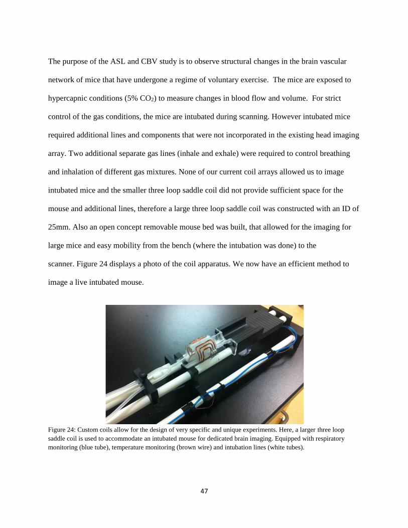
47
The purpose of the ASL and CBV study is to observe structural changes in the brain vascular
network of mice that have undergone a regime of voluntary exercise. The mice are exposed to
hypercapnic conditions (5% CO2) to measure changes in blood flow and volume. For strict
control of the gas conditions, the mice are intubated during scanning. However intubated mice
required additional lines and components that were not incorporated in the existing head imaging
array. Two additional separate gas lines (inhale and exhale) were required to control breathing
and inhalation of different gas mixtures. None of our current coil arrays allowed us to image
intubated mice and the smaller three loop saddle coil did not provide sufficient space for the
mouse and additional lines, therefore a large three loop saddle coil was constructed with an ID of
25mm. Also an open concept removable mouse bed was built, that allowed for the imaging for
large mice and easy mobility from the bench (where the intubation was done) to the
scanner. Figure 24 displays a photo of the coil apparatus. We now have an efficient method to
image a live intubated mouse.
Figure 24: Custom coils allow for the design of very specific and unique experiments. Here, a larger three loop
saddle coil is used to accommodate an intubated mouse for dedicated brain imaging. Equipped with respiratory
monitoring (blue tube), temperature monitoring (brown wire) and intubation lines (white tubes).

48
3.4 Summary
Mice are the mammals of choice in the laboratory for cancer and genetic studies because they can
be manipulated genetically. MRI offers a method to quantify and track possible changes in models
using imaging. To ensure findings are statically meaningful, many mice must be imaged for a
particular study. MMMRI offers a solution, where multiple mice are imaged simultaneously. This
makes it possible to undertake large mouse studies in a reasonable time frame. There have been
many RF configurations of MMMRI, however possible transmit and shielding configurations have
not yet been explored. The purpose of this thesis was to investigate possible RF configurations to
image the brains of multiple live mice.
The study began with designing a multiple loop saddle coil that proved to provide increased SNR
and sufficient B1 homogeneity over the mouse brain. Following, four possible RF configurations
were explored, resulting in a Tx-Rx saddle coil without shielding. This prompted an investigation
of coupling between exposed coils through a mechanism of mutual inductance. It was shown that
coupling could be minimized through two means, i) rotating adjacent coils and ii) separating the
coils, both of which resulted in increased image quality. The final multiple live imaging array was
then designed using a minimization algorithm which minimized mutual inductance between all
seven coils in the array. The array resulted in only a 6% loss in image quality when compared to a
single coil. High resolution images (90µm) were acquired and a modified SENSE reconstruction
method allowed single images to be properly reconstructed and analyzed. Alternatively, the added
sensitivity could be used to reduce scan time or allow for other types of scanning protocols such
as BOLD imaging which requires high SNR.

49
Possible improvements with the current array may include incorporating capacitive coupling (in
addition to mutual inductance) minimization which may further decrease coupling and improve
image quality. Also, the multiple loop saddle coil may be further optimized by configuring a
possible quadature design and investigating the configuration and number of segmentation
capacitors. In addition, we limited our design to seven coils (samples). Further investigations could
be done to accommodate more coils, which would inherently have more coupling and a different
solution. In this thesis only one type of pulse sequence was used, a gradient echo. Experiments
need to be completed with different pulses sequences (for example a spin echo) where coil
coupling on transmit could result in image artifacts and poor image quality. Finally, the benefits
of having a higher resolution and SNR still need to be investigated. For example, in the detection
of anatomical brain differences between groups of mice, perhaps higher resolution may show
differences not previously seen with lower resolution images.
50
References
1. R.M. Henkelman. Systems Biology through Mouse Imaging Centers: Experience and New
Directions. Annual Review of Biomedical Engineering 12:143:166, 2010.
2. B.J. Nieman, M.D. Wong, R.M. Henkelman. Genes into Geometry for Mouse Development in
3D. Current Opinion in Genetics and Development 21:638-646, 2011.
3. Nadeau JH, Balling R, Barsh G, Beier D, Brown SDM, Bucan M, Camper S, Carlson G,
Copeland N, Eppig J, Fletcher C, Frankel N, Ganten D, Goldowitz D, Goodnow C, Guenet J,
Hicks G, Hrabe de Angelis M, Jackson I, Jacob HJ, Jenkins N, Johnson D, Justice M, Kay S,
Kingsley D, Leharch H, Magnuson T, Meisler M, Poustka A, Rinchik EM, Rossant J, Russell LB,
Schimenti J, Shiroishi T, Skarnes WC, Soriano P, Stanford W, Takahashi JS, Wurst W, Zimmer
A. Functional annotation of mouse genome sequences. Science;291:1251–1255, 2001.
4. Moats RA, Velan-Mullan S, Jacobs R, Gonzalez-Gomez I, Dubowitz DJ, Taga T, Khankaldyyan
V, Schultz L, Fraser S, Nelson MD, Laug WE. Micro-MRI at 11.7 T of a murine brain tumor
model using delayed contrast enhancement. Mol Imaging;2:150–158,2003
5. Bock NA, Zadeh G, Davidson LM, Qian B, Sled JG, Guha A, Henkelman RM. High-resolution
longitudinal screening with magnetic resonance imaging in a murine brain cancer model.
Neoplasia, 2003; 5(6): 546–554.
6. L.M. Gazdzinski, B.J. Nieman. Cellular Imaging and Texture Analysis Distinguish Differences in
Cellular Dynamics in Mouse Brain Tumors. Magn. Reson. Med. (2013)
7. B.J. Nieman, J.B. Bishop, J. Dazai, J.P. Lerch, A. Feintuch, J.G. Sled, R.M. Henkelman. MR
Technology for Biological Studies in Mice. NMR in Biomedicine 20(3):291-303, 2007.
8. N.A Bock, N.B Konyer, R.M. Henkelman. Multiple Mouse MRI. Magn. Reson. Med. 49(1):158-
167, 2003.
9. N.A Bock, B.J. Nieman, J.B. Bishop, R.M. Henkelman. In Vivo Multiple Mouse MRI at 7 Tesla.
Magn. Reson. Med. 54(5):1311-1316, 2005.
10. J.P. Lerch, J.G. Sled, R.M. Henkelman. MRI Phenotyping of Genetically Altered Mice. Method
in Molecular Biology 711:349-361, 2011.
11. J.E. Bishop, S. Spring, J. Dazai, B.P. Chugh, S. Portnoy, S. Suddarth, G.R. Morris GR, R.M.
Henkelman. Multiple mouse imaging of 16 live mice. Proceedings of the 16th Annual Meeting
ISMRM, Toronto, ON, Canada,1176, 2008.
12. X. Zhang, J.E. Schneider, S. Portnoy, S. Bhattacharya, R.M. Henkelman. Comparative SNR for
High-Throughput Mouse Embryo MR Microscopy. Magn. Reson. Med. 63:1703–1707, 2010.
13. M. Mitsuda, M. Yamaguchi, T. Furuta, A. Nabetani, A. Hirayama, A. Nozaki, M. Niitsu, H. Fujii.
Multiple-animal MR Imaging using a 3T Clinical Scanner and Multi-channel Coil for Volumetric
Analysis in a Mouse Tumor Model. Magnetic Resonance in Medical Sciences: 10(4): 229-237,
2011.
14. A. Nabetani, M. Yamaguchi, A. Hirayama. Multiple-animal MR imaging performed using a 3-
Tesla whole-body scanner: A feasibility study using a 16-chanel array coil. Proc Intl Soc Mag
Reson Med; 18:1488, 2010.
15. P.B Roemer, W.A. Edelstein, C.E Hayes, S.P. Souza, O.M. Mueller. The NMR phased array.
Magn. Reson. Med:16(2): 192–225, 1990.
16. K.P. Pruessmann, M. Weiger, M.B. Scheidegger, P. Boesiger. SENSE: sensitivity encoding for
fast MRI. Magn. Reson. Med; 42(5): 952–962, 1999.
51
17. M.S. Ramirez, E. Esparza-Coss, J.A. Bankson. Multiple-mouse MRI with multiple arrays of
receive coils. Magn. Reson. Med; 63(3): 803–810, 2010.
18. M.S. Ramirez, S.Y. Lai, J.A. Bankson. A throughput-optimized array system for multiple-mouse
MRI. NMR Biomed; 26: 237–247, 2013.
19. Y. Matsuda, S. Utsuzawa, T. Kurimoto, T. Haishi, Y. Yamazaki, K. Kose, I. Anno, M. Marutani.
Super-Parallel MR Microscope. Magn. Reson. Med; 50:183–189, 2003.
20. D.G. Nishimura. Principles of Magnetic Resonance Imaging. Lulu 1.1, 2010.
21. F. D. Doty, G. Entzminger, J. Kulkarni, K. Pamarthy and J.P. Staab. Radio frequency coil
technology for small-animal MRI. NMR Biomed; 20: 304–325, 2007.
22. D.I. Hoult, R.E. Richards. The Signal-to-Noise Ratio of the NMR Experiment. J. Magn. Reson;
24: 71–85, 1976.
23. D.I. Hoult. Sensitivity of the NMR Experiment. In Encyclopaedia of NMR Vol. 7. Wiley:
Chichester; 4256–4266, 1996.
24. J.S. Tropp. Radiation damping and reciprocity in magnetic resonance reception. Presented at 12th
ISMRM. Poster 1646. Kyoto, 2004.
25. E. Fukushima, B. Stephen, W. Roeder. Experimental pulse NMR, A nuts and bolts approach.
Addison Wesley p.297 386,1981.
26. D.I. Hoult. The NMR receiver: a description and analysis of design. Progress in NMR
Spectroscopy; 12: 41–77, 1978.
27. J.J.H. Ackerman. Surface (local) coils as NMR receivers. Concepts in Magnetic Resonance; 2: 23–
42, 1990.
28. J. Hyde. Surface and other local coils for in vivo studies. In Encyclopaedia of NMR Vol. 7. Wiley:
Chichester, ;4656–4664, 1996.
29. B.H Suits, A.N. Garroway, J.B. Miller. Surface and gradiometer coils near a conducting body: the
lift-off effect. J. Magn. Reson; 135: 373–379, 1998.
30. W.A. Edelstein, C.J. Hardy, O.M. Mueller. Electronic decoupling of surface-coil receivers for
NMR imaging and spectroscopy. J Magn Reson; 67: 156–161, 1886.
31. Tropp J. Mutual inductance in the birdcage resonator. J Magn Reson; 126: 9–17, 1997.
32. W. Edelstein. RF Systems and Coils for MRI and MRS. In Encyclopaedia of NMR Vol 6. Wiley:
Chichester, 3950-3954, 1996.
33. Y. Li, A.G. Webb, S. Saha, W.W. BreyW, C. Zachariah, A.S. Edison. Comparison of the
performance of round and rectangular wire in small solenoids for high-field NMR. Magnetic
Resonance in Chemistry; 44: 255–262, 2006.
34. D.M. Ginsberg, M.J. Melchner. Optimum geometry of saddle shaped coils for generating a
uniform magnetic field. Rev. Sci. Instrum; 41: 122–123,1970.
35. F.D. Doty, G. Entzminger Jr. Center-fed paralleled saddle coils for multinuclear double-
resonance NMR or MRI. U.S. Pat. 6,175,237, 2001.
36. C.E. Garrido-Salomon, E.L. Vidoto, M.J. Martins, A. Tannuns. Optimization of saddle coils for
magnetic resonance imaging. Braz J Phys 36(1A):4–8, 2006.
37. W. Domingguez-Viqueira, W. Berger, J. Parra-Robles, G.E. Santyr. Litz Wire Radiofrequency
Receive Coils for Hyperpolarized Noble Gas MR Imaging of Rodent Lungs at 73.5 mT Concepts
in Magnetic Resonance Part B: Vol. 37B(2) 75–85, 2010.
38. C.M. Collins, L. Shizhe, X. Qing, M.B. Smith. A Method for Accurate Calculation of B1 Fields
in Three Dimensions, Effects of Shield Geometry on Field Strength and Homogeneity in the
Birdcage Coil. Magn. Reson. Med. 125(1):233-241, 1997.
39. J.E. Dennis. Nonlinear Least-Squares. State of the Art in Numerical Analysis ed. D. Jacobs,
Academic Press, pp. 269–312. 1977.

52
40. B.J. Nieman, N.A. Bock, J. Bishop, J.G. Sled, X. J. Chen, R.M. Henkelman. Fast Spin-Echo for
Multiple Mouse Magnetic Resonance Phenotyping. J. Magn. Reson; 54: 532–37, 2005.
41. S.C. Kale, J. P. Lerch, R.M. Henkelman, X.J. Chen. Optimization of the SNR-Resolution Trade
off for Registration of Magnetic Resonance Images. Human Brain Mapping; 29: 1147-58, 2008.