1

Comparison of hindcasted extreme waves with a Doppler radar measurements in the North Sea.

S. Ponce de León, João H. Bettencourt and F. Dias

School of Mathematics and Statistics, UCD Earth Institute,

University College Dublin Ireland

Corresponding author:

sonia.poncedeleonalvarez@ucd.ie

Abstract

Extreme sea states have been recorded in the North Sea during several winter periods in which significant wave heights of 10 m or more were common. These sea states present a challenge to wave forecasting systems and a threat to offshore installations such as oil and gas platforms and windmill parks. In this work, we study the ability of a 3rd generation spectral model in reproducing the extreme sea states. Times series and directional wave spectra measured and modeled are compared for a 10 day period in the winter of 2013-2014 where successive severe storms moved across the North Atlantic and the North Sea. Records were obtained from a Doppler radar and wave buoys. The hindcast was performed with the WAVEWATCH III (WW3) model (Tolman 2014) with high resolution both in frequency and direction. A good agreement was obtained in general for integrated parameters, but discrepancies were found to occur in spectral shapes. This study also highlights that the wave model significantly underestimated the directional spreading, with differences reaching 24° which can compromise the ability of the wave model to accurately predict extreme waves. 1 Introduction

The North Sea wave climate varies from gentle to rogue and it was previously studied by

different authors (Boukhanovsky et al., (2007), Reistad et al., (2011), Ponce de León and

Guedes Soares (2012)). Activities in the North Sea are diverse and include fisheries, oil and

gas industry, shipping and wind power device installations for obtaining green energy.

However, extreme sea states generated under hurricane force storms are becoming more

frequent in the North Sea (Behrens and Gunther (2009)). Rogue waves have been recorded and

studied, indicating how the appropriate conditions for rogue waves differ depending on the

location under consideration (Magnusson and Donelan (2013); Haver and Andersen 2000;

Haver 2000).

2

A source of generation of extreme wave groups is the wind gustiness in the North Sea. Strong

winds feeding a wave group for a long time period could be the reason of enormous growth of

individual wave height within a certain group (Plekachevsky et al., 2012; Kettle 2015).

Waseda et al., (2011) found that during freakish sea states (Waseda et al., 2014; Tamura et al.,

2009) the average directional spreading can be lower than for non-freakish sea states, in a study

based on 20 minute wave records during the winter months of 2003-2005 in the North Sea and

in a hindcast produced with the WW3 model.

The robustness of a wave forecast is of a great importance for avoiding economical and human

losses. The knowledge about extreme waves and their study is a very important challenge to

the scientific community, for reasons related with the scientific understanding of their causes

and how they propagate and disappear as well as for the safety of navigation and of prevention

of damage to offshore structures and ships.

The present study analyses severe storms generated in the winter of 2013-2014. The attention

was focused in the North Sea where high resolution hindcasts were conducted by applying the

WW3 model (version 4.18). A Doppler wave radar mounted at the Sleipner platform provided

wind and wave records that were taken as a reference to analyse the directional spreading, an

important spectral parameter in the forecast of extreme sea states and which plays an important

role in the definition of the shape of the wave spectrum.

In section 2, we describe briefly the North Sea. Section 3 treats the details of the WW3 model

configuration used for the hindcast. In Section 4, details are given about the recorded data used.

Sections 5 and 6 present the results and discussion where a comparison of unidimensional and

directional wave spectra and the spectral parameter of directional spreading retrieved from the

MIROS radar and from WW3 is given. The conclusions are given in section 7.

2 Region of study

The North Sea, due to its complex geometry and bathymetry, reveals complicated synoptic

conditions, wind waves and currents patterns. Surrounded by several coastal sections and

connected to the North Atlantic Ocean and the Baltic Sea, the North Sea is in itself a particular

natural laboratory for the study of extreme waves. High waves are often generated by low

atmospheric pressure and strong wind associated with storms. Due to the North Sea geometry,

severe winds from different directions have a large impact in the coastal regions (De Winter et

3

al., 2013).

The north part of the North Sea is characterized by deep waters and the central and south parts

are mainly intermediate waters ranging from 50 to 75 m where most of the oil platforms are

located. Figure 1 shows the geographical domain of the high resolution nested grid with all the

locations where the hindcast was verified with the measured data. Most of these locations are

in deep waters except for locations 9 (60 m) and 10 (30 m).

A characterization of the winter period of 2013-2014 was given in the Met Office Report 2014.

The most remarkable characteristic was the extraordinary duration of the successive storms

and the clustering of deep depressions. A hindcast study with emphasis on the Hercules storm

of January 2014 and its effects on the Iberian Peninsula was discussed in Ponce de León and

Guedes Soares (2015).

3 The WW3 model set up

WW3 (Chawla et al., 2013; Tolman 2014) is a third generation wave model developed at

NOAA/NCEP based on the WAM model (Komen et al., 1994). Ocean wave models such as

WW3 are based on the spectral energy action balance equation (1),

����,��

��+ � ∙ �����, �� + �,� ∙ ��,����, �� = ���, �� (1)

where f and θ are the spectral frequency and direction, respectively and F is the spectrum, ��

and ��,� are the characteristic velocities in the physical and spectral spaces, respectively and �

and �,�are the gradient differential operators. S is the source function (equation 2) in which

all the physical processes considered in WW3 are represented. There are three main

contributions to S: Sin-wind input, Snl-wave-wave nonlinear interactions, Sds-dissipation of the

wave energy (wave breaking and shallow water processes),

� = ��� + ��� + ��� (2) The computational coarse grid domain was set to 80º N, 18º N, 90º W, 30º E (Fig. 2, left) at

spatial resolution of 0.25º (about 27 km) covering almost the entire part of the North Atlantic.

The first nested grid (intermedium grid in Table 1) was defined for a region with the following

limits: 66.0º N, 47º N, 35º W, 12.875º E (Fig. 2) at the spatial resolution of 0.125º (16 km).

4

The high spatial resolution nested grid was defined over the North Sea region with a resolution

of 0.0625º (6.95 km) covering the region 63º N, 48º N, 9º W, 7.375º E (Fig. 3). Other numerical

parameters are detailed in Table 1.

The hindcast was performed for two months and 15 days for the winter of 2013-2014. The

wave model was driven by 1 hourly wind fields from the ECMWF operational forecast (high

resolution model) from the MARS archive with a horizontal resolution of 0.125º (16 km) and

137 vertical levels.

The bathymetry data comes from the GEODAS NOAA’s National Geophysical Data Centre

(NGDC), with a resolution of 1 minute of degree in latitude and longitude which was linearly

interpolated to the three level model grids. The wave spectrum is provided for 36 directional

bands, and 30 frequencies from the minimum frequency of 0.0350 Hz up to 0.5552 Hz.

The shallow water model was considered only for the nested grid over the North Sea (Table 1).

Regarding the physical and numerical aspects, the following processes and parameters were

activated for the North Sea grid: wind input and dissipation of energy of WAM cycle 4

(ECWAM), JONSWAP bottom friction formulation, the lumped triad interactions method

based on the stochastic model of Eldeberky (1996), the discrete interaction approximation

(DIA), depth induced breaking of Battjes and Janssen (1978) with a breaking threshold of 0.73,

refraction and for the propagation of the spectral wave energy along the geographical domain

a third order propagation scheme was chosen using the averaging Tolman’s (2002) technique.

Reflection, ice and currents were not considered in this hindcast.

Table 1. Numerical definition of the WW3 configuration.

Parameters Coarse grid North Atlantic Intermedium nested grid High resolution nested

Geographical limits 80ºN, 18ºN, 90ºW, 30ºE 66.0ºN,47ºN,35ºW,12.875ºE 63ºN,48ºN,9ºW,7.375ºE

Spatial resolution 0.25º 0.125º 0.0625º

Number of points (481,249)119769 (401,153)61353 (289,241) 69649

Type of spectral model

deep water deep water shallow water

Propagation Spherical Spherical Spherical

Wind input (Sin) Janssen (1989, 1991) Janssen (1989, 1991) Janssen (1989, 1991)

White capping dissipation

Komen et al. (1984) Komen et al. (1984) Komen et al. (1984)

Nonlinear Interactions (Snl)

Four wave-wave nonlinear interactions

Four wave-wave nonlinear interactions

Triad interactions Eldeberky (1996)

Bottom friction dissipation (Sbofr)

JONSWAP JONSWAP JONSWAP

5

Wind input time step (hour)

1 1 1

Wave model output time step (hour)

1 1 1

Integration time step (seconds)

120 60 30

Wind data ECMWF operational forecast

ECMWF operational forecast

ECMWF operational forecast

Bathymetry data GEODAS NOAA’s GEODAS NOAA’s GEODAS NOAA’s

SIN3 maximum value of wind-wave

coupling

BETAMAX=1.40 BETAMAX=1.40 BETAMAX=1.40

4 Data

4.1 Norwegian MIROS radar

The Miros SM-050 wave and current radar is a purpose-built pulse Doppler radar system,

designed for real-time measurement of directional ocean waves and surface current. The

MIROS radar is mounted on the fixed platform (Sleipner) which recorded averaged wave

observations and wave spectra. Radar data was available at every 10 minutes for Sleipner

(location 5, Figure 1) during 10 days (20th-31st December 2013). The radar records were

compared to a wave buoy and WW3 model output.

The radar observes the ocean surface in a semi-circle at a distance of 180-450 m depending on

the installation height, typically 25 – 80 m. Six 30º sectors are scanned in sequence. The

observation footprint is 75 m deep horizontally. The radar has the following system

performance measurements characteristics to record the directional wave spectra: directions:

36, directional resolution: 10º, frequencies: 37, frequency resolution: 0.01 Hz, frequency range:

0.0312 - 0.3125 Hz, update interval: 2.5 minutes and an averaging time: 45 minutes default.

More details can be found at http://www.miros.no.

4.2 Wave buoys JCOMM Project

Wave buoys at ten different locations were available and distributed by the JCOMM-Joint

Technical Commission for Oceanography and Marine Meteorology Project (Bidlot, 2012).

These moorings consist of directional and non-directional wave buoys transmitting hourly data

on the standard suite of meteorological parameters. Mean wave direction was recorded only in

6

one of the wave buoys (location 10). Quality controls were performed on the wave buoy

datasets and a number of errors were identified and corrected accordingly.

The statistical parameters employed in the validation of the hindcast against the wave buoys

are the correlation coefficient, bias and scatter index. The bias is defined as the mean of the

residual, which is the difference between the buoy data and model data and the scatter index is

defined as the standard deviation of the model data from the best fit line, divided by the mean

observation. The validation for the modelled Hs retrieved from the high resolution nested grid

(Table 1) was performed against the ten wave buoys averaged records of JCOMM.

The statistical parameters revealed a good agreement of the modelled data with a linear

correlation. The correlation coefficients were in the range of 0.850 (location 10) and 0.961

(location 2) and the scatter indexes were in the range from 0.11 (location 2) up to 0.292

(location 10). The bias turned out to be negative (records were taken as reference) in five

locations (3, 4, 6, 7, 9) indicating that the WW3 model overestimates the recorded values of

Hs at those locations.

Figure 1. The North Sea bathymetry, the WW3 ten output locations and wave buoys. 1-Gullafks, 2-North Alwyn, 3-Troll, 4-Heimdal, 5-Sleipner, 6-Mungo, 7-Ulla, 8-Ekofisk, 9-Valhall, 10-Fino1. The lowest correlation (0.85) and the highest scatter index (0.292) were obtained at location 10

(FINO1) placed in intermediate waters at 30 meters of depth which could be a possible reason

for the obtained low correlation.

7

In addition, the wind speed from the ECMWF atmospheric high resolution model used in the

hindcast was verified against the recorded buoys data across the North Sea (Figure 1). The

obtained correlation coefficients were in the range from 0.9612 (location 7) up to 0.9403

(location 5), bias from 0.0357 (location 8) up to -0.9729 (location 5) and scatter indexes from

0.0891 (location 7) up to 0.1434 (location 5). The correlation of the location 10 was affectec

by the fact that the number of the recorded values was 1627 instead the 1824 values which

should be for the study period (two months and 15 days). In general, a good agreement between

the wind speed from the buoys and from the high resolution ECMWF wind model was obtained.

Table 2. Statistical parameters for the Hs at the numbered locations: 1-Gullafks, 2-North Alwyn, 3-Troll, 4-Heimdal, 5-Sleipner, 6-Mungo, 7-Ullabnor, 8-Ekofisk, 9-Valhall, 10-Fino1 (See Fig. 1). Cc-correlation coefficient.

Location Bias Scatter index Cc

1 0.289 0.137 0.938

2 0.056 0.111 0.961

3 -0.096 0.179 0.892

4 -0.296 0.146 0.910

5 0.277 0.137 0.949

6 -0.212 0.129 0.922

7 -0.167 0.130 0.948

8 0.094 0.136 0.951

9 -0.135 0.131 0.960

10 0.064 0.292 0.850

5) Results

5.1) Characterization of the winter storms of December 2013

An intense depression passed to the north of the UK on the 24th of December of 2013,

recording a mean sea level pressure of 936 mb (Met Office Report 2014). Pressures below 950

mb for UK land stations were reported as rare and it was the lowest value at a UK land station

for many years. The ECMWF wind fields from the coarse grid (left panel) and intermedium

nested grid (right panel), respectively, show stormy conditions over the North Sea on 25th

8

December 2013 at 05 UTC where the wind speed reached values of about 25 m/s (Figure 2).

Figure 2. ECMWF hourly operational forecast wind archive on the coarse and intermedium nested grids limits on the 25th December 2013 at 05 UTC.

Because the winter period of this study was characterized by successive severe storms derived

from low pressure systems that crossed the North Atlantic, consequently in the North Sea the

strong wind had a direction from SW and South in accordance with the cyclonic circulation.

At the beginning of December 2013, from the 5th and up to the 6th at 18 UTC very strong

winds from the NW (higher than 25 m/s), blew along the main axis of the North Sea where the

fetch is larger generating Hs of about 10 m (Figure 3, left) at location 5 (Sleipner). This storm

moved towards Norway with the strongest winds blowing across the North Sea (Figure 4).

From the 20th up to the 29th the wind blew mainly from the SW towards Norway where the

fetch is shorter. However in at the north part of the North Sea, on the 25th of December, the

wind speed and Hs were noticeably high (Figure 4), reaching approximately 25 m/s and values

above 8 m, respectively.

Figure 3. Time series comparison for the period of the study (left) and comparison between the Hs

retrieved from the MIROS radar, WW3 and JCOMM wave buoy at Sleipner (right).

9

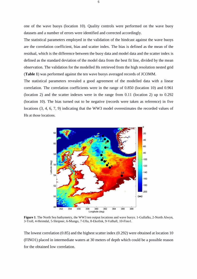
Figure 4. ECMWF wind speed (m/s) (left) and the WW3 Hs (m) map from the high resolution nested grid on the 25th December 2013 at 05 UTC.

5.1.1 Wave roses

As wave directional data was missing at nine of the ten wave buoys in the North Sea, only the

directional data from the WW3 model is analysed. The good performance of WW3 based on

the low scatter indexes and high correlations supports the directional analysis below. Wave

roses (Figure 5) were constructed using the output of the wave model from the high resolution

nested grid. The wave rose spokes point in the direction from which the waves propagate. At

each of the ten locations (only three representative roses for the North, central and South parts

of the North Sea are shown), most of the spokes are pointing in a southerly direction. The

largest spokes were pointing in a south easterly or south westerly direction, meaning that for

the most of the time waves propagated from south to north. It seems that the significant wave

height increases with latitude, for waves propagating from south to north, because in this

direction the fetch is larger.

This analysis allows to characterize the wave climate during a peculiar winter (2013-2014)

dividing the North Sea in three main regions: North (locations 1, 2, 3), central (4, 5, 6, 7) and

southern (8, 9, 10) parts (Figure 5). Locations 1 and 3 presented very similar wave roses with

the highest percentage of waves coming from the South and South East sectors with 3-6 m and

10

6-9 m of Hs. Only a small part of Hs higher than 9 m were observed from the North West sector.

On the case of location 2, the majority of the waves came from the SE sector and were in the

range of 3-6 m and 6-9 m of Hs.

The central part of the basin was characterized by the wave roses of locations 4, 5, 6, 7 for

which locations 6 and 7 presented similar wave roses showing a high occurrence of waves

propagating from the SW sector (Hs in the range of 3-6 m and 6-9 m) and only a few cases

were higher than 9 m from NW. Locations 4 and 5 which were more in the centre of the North

Sea were characterized mainly by waves coming from the South East and South West with Hs

on the range of 6-9 m and 3-6 m.

The south part of the North Sea was characterized with the wave roses of locations 8, 9, 10

(Figure 5). It seems that the South is less energetic than the central and the northern part of the

North Sea. Locations 8, 9 and 10 show almost the same proportion of the waves in the range

from 0-3 m and 3-6 m coming from the SW and again the highest Hs, with values of 9 m or

higher, come from the NW sector.

This suggests that while waves propagating from a northerly direction are infrequent, their

significant wave height is much more likely to be above 9 metres than waves propagating from

a southerly direction.

11

Figure 5. Wave roses (WW3 data) for the period of 1st December 2013 up to 15th February 2014. From North to South North part of the basin (top panels): left location 1, middle-location 2, right-location 3. Central part of North Sea: Middle panels: left-loc5, middle-location 6, right-location 7. South part (bottom panels): locations 8,9,10, respectively.

6) Discussion

6.1 Frequency spectra at Sleipner

The comparison of the time series for the U10 is depicted in Figure 6A. The evolution in time

of the wind speed at 10 meters (U10) height shows two maxima, the first one of 21.66 m/s

(MIROS) and 21.25 m/s (ECMWF model) on the 25th December 03 UTC and the second one

of 21.06 m/s (MIROS radar) and 19.59 m/s (ECMWF wind) on 27th December at 07 UTC

corresponding to two different storms.

The time series for the Hs clearly show the duration of the first and second storms (Figure 6B).

The highest Hs value recorded by the radar was 8.02 m on 25/12/2013 at 05 UTC (Figure 6B).

However, the wave model underestimated the Hs (7.28 m). The second maximum took place

12

on the 27/12/2013 at 20 UTC and it is 7.07 m (radar) and 6.67 m (model).

The highest errors measured by the RMS difference between radar and model frequency

spectrum (highlighted by the dashed vertical lines in Figure 6C) were obtained during the two

storms as can be seen. Thus, we focused our attention to those dates where these errors were

high by analysing the one dimensional spectra and their respective source functions.

Figure 6. Time series of A) U10 (m/s); B) Hs (m), C) Root mean square (RMS) error of WW3 frequency spectra for the period of 20/12/2013 up to 31/12/2013. RMS error computed by interpolating radar spectra to WW3 frequency grid (in the common frequency range). Dashed vertical lines at 25/12/2013 04 UTC, 28/12/2013 05 UTC and 30/12/2013 23 UTC. Red line-recorded by radar; dashed black line-WW3.

The discrepancies between radar and model frequency spectra during the two storms can be

attributed to a slight shift of the spectral peaks in the case of the spectrum of 25th September

2013 at 04 UTC (Figure 7) and in the spectrum of the 28th of December at 05 UTC (Figure

8). In both cases the dominant local processes in the spectral energy balance are wind input and

nonlinear interactions (Figure 10A) and B)), whose distributions with frequency are such as to

13

inject energy in the low frequency range at and below the peak frequencies.

The second cause of error is a difference in the level of spectral energy at the peak frequency

(Figure 9). In the case of the pronounced underestimation of the wave model on the 30th of

December of 2013 at 23 UTC, the dominant local process was the four-wave non-linear

interactions (Figure 10C). The non-linear interactions (Snl) play the principal role in the

adjustment of the total source balance as was demonstrated in Tamura et al., (2010). In addition,

there are some differences in the variance density spectra at the high frequency tail of the

spectra, especially at the last two dates where secondary peaks are clearly visible in the radar

spectra while they are absent in the WW3 spectra.

Figure 7. Frequency spectra at Sleipner on the 25th of December at 04 UTC. A) Radar and WW3 spectra. B) Difference between radar and WW3 spectra.

14

Figure 8. Frequency spectra at Sleipner on the 28th of December at 05 UTC. A) Radar and WW3 spectra. B) Difference between radar and WW3 spectra.

Figure 9. Frequency spectra at Sleipner on the 30th of December at 23 UTC. A) Radar and WW3 spectra. B) Difference between radar and WW3 spectra.

15

Figure 10. Source functions (WW3) for the A) 25/12/2013 at 04 UTC; B) 28/12/2013 at 05 UTC; C) 30/12/2013 at 23 UTC. Sin is wind input, Snl is nonlinear interactions, Sbreak is breaking dissipation, Sbot is bottom friction dissipation and Stot is total source function magnitude.

Since the location 5 (Sleipner) is at a deep water location the bottom friction dissipation (Sbot)

does not play any role. In the case of the storms of 25th and 28th December 2013, the Snl played

a secondary role in the spectral balance; on the contrary, for the 30th of December, where the

wind speed was a breeze of about 10 m/s, it can be seen that Snl prevailed and reacted quickly

to changes in the source balance.

However, it is necessary to point out that the temporal variations of the wave spectrum are

determined not only by the source functions but also by the propagation term. The analysis of

the effect of advection is underway and we expect to report on this soon.

6.1 Directional spreading

Directional spreading is one of the parameters together with the steepness and the frequency

16

bandwidth which characterize the geometry of a directional wave spectrum. We compared the

directional spreading from the wave model to the one recorded by the MIROS radar during the

period of study. Prominent differences for the directional spreading were found. The highest

differences between the hindcast and radar values were found during the first storm that

occurred approximately between the 24th and the 26th of December of 2013, according to the

wave records (Figure 6B).

Radar records of the directional spreading parameter were taken as a reference and for the first

storm these differences are higher than for the second storm (Figure 11). For the first one the

differences ranged from 10º up to 23.47º and for the second one ranged between 10º and 18.48º.

The duration of the storms was almost two days. This means that the radar recorded higher

values than the model for both storms. These differences are very important for the prediction

of extreme sea states.

False extreme sea states or false freak waves can be derived from a hindcast or a wave forecast

if the model produces lower directional spreading than in reality. The reasons for the obtained

differences are not clearly understood yet. A possible interpretation is that the radar is showing

complex wave systems of the North Sea that the wave model cannot reproduce.

The implications of these differences in the directional spreading parameter are reflected in the

bidimensional wave spectra (Figure 13 and 14). The findings of poor representation of the

directional spreading affect the transition from a normal to dangerous sea state in a wave

forecast.

Tamura et al., (2010) obtained similar findings for an oceanic location in the Pacific Ocean.

However, their results showed that during the period of the study (two months) the hindcasted

directional spreading parameter was higher than the recorded values. In our case, the directional

spreading values recorded by the radar were available for a shortest period of ten days and

resulted higher most of the time than the modelled values (Figure 11).

The normalized directional distribution of spectral energy is shown in Figure 12 for the two

dates where the difference between radar and model were larger. For the 25th of December at

13 UTC the radar shows a multimodal distribution with two peaks whereas the model shows

only one significance peak, with a small secondary maxima. On the 26th of December at 01

17

UTC, both in the radar and the model, a growth in the secondary peak can be observed but the

model still shows considerable deviations from the radar distribution.

Figure 11 Parameter directional spreading (º) time series from the wave model (red line) and from the MIROS radar (black line). Period: 20th-31st December 2013 (left). Differences between the directional spreading recorded by radar (reference) and obtained from WW3 (right).

Figure 12. Normalized directional distribution of wave spectral energy. A) 25/12/2013 13 UTC; B) 26/12/2013 01 UTC. Red – Radar; Black –WW3.

18

6.1.2) 2d spectra

In this section we inspect the directional wave spectra retrieved from the radar and from WW3

at two dates identified above for which the directional spreading differences are higher (Figure

11). An important characteristic to be highlighted is that, in general, all of the WW3 directional

spectra analysed, coincident with the MIROS radar spectra dates, are broader than the observed

spectra (Figure 13 and 14), which also was remarked by Babanin et al., (2010) and Tamura et

al (2010).

On the 25th of December at 13 UTC, directional spreading difference between radar and WW3

attains a maximum of 23.5°. The directional spectrum for this date is shown in Figure 13,

where it can be observed that, while the peak frequency is similar between radar and model,

the WW3 peak direction is ~ 45° to the east of the radar spectrum peak direction. Total energy

is similar, judging from Hs values but the radar spectrum covers a sector with width of 135°

from southwest to east, while the model spectrum is limited to the southeast sector.

Additionally, in the radar spectrum, a secondary non-zero energy level can be observed

propagating in the opposite direction to the main wave system.

Figure 13. Directional wave spectra on the 25/12/2013 at 13 UTC. A) Radar; B) WW3.

19

Figure 14. Directional wave spectra on the 26/12/2013 at 01 UTC. A) Radar; B) WW3.

For the 26th of December at 01 UTC, radar and WW3 spectra are displayed in Figure 14. The

model shows a single peaked spectra with southeast peak direction while the radar shows a

peak direction south-southwest. The situation is similar to Figure 11, with peak frequencies ~

0.1 Hz for both radar and WW3 but a substantial difference in the peak direction is found,

together with a radar spectra spread through a 180° sector, while the model spectra is limited

to the southeast sector. Secondary peaks, both in frequency and direction spaces are visible in

the radar spectra.

7) Conclusions

The skill of a 3rd generation wave model in hindcasting extreme sea states was assessed for a

10 day winter period in the North Sea using buoys and Doppler radar records. Integrated

parameters of the sea state spectrum were accurately hindcasted by the model. The frequency

spectra of the model was compared to the one measured by the radar by means of the RMS

difference and a good agreement was found in general, but the RMS difference showed large

20

differences at the peak of two storms. These differences were attributed to a slight shift in the

peak frequency and an underestimation of the peak spectral energy. In this last case, the

dominant local process were nonlinear interactions, while the wind input was an additional

dominant source term in the previous cases.

When forecasting extreme waves in a directional sea, the directional spreading of the spectrum

is an important parameter. It was found that the model consistently underestimated the

directional spreading when compared to the value of the radar. The most severe

underestimation occurred near or at the peak of the storms, which aggravates the need to clarify

the source of these discrepancies because these are the most dangerous sea states, where the

appearance of extreme waves can be associated to severe risks to marine structures and

operations.

Ongoing work is devoted to reveal the source of these discrepancies in the directional spreading

estimated by the model and also on the more general source term balance in the wave spectrum.

In particular, the hindcast will be repeated for selected time windows during these 10 days with

a more advance method to better estimate the non-linear source term. Osborne (2013) found

that the nonlinear interactions computed by DIA in the WW3 leads to an underestimation of

the spectral wave energy.

Acknowledgements The authors are very grateful to STATOIL and Dr. Anne Karin Magnusson and Dr. Magnar Reistad from the Norwegian Meteorological Institute who kindly supplied the MIROS radar records. This work was supported by the European Research Council (ERC) under the research project ERC-2011-AdG 290562-MULTIWAVE and Science Foundation Ireland under grant number SFI/12/ERC/E2227. http://www.ercmultiwave.eu/

References

Babanin A.V., Tsagareli K.N., Young I.R., Walker D.J., 2010. Numerical investigation of spectral evolution of wind waves, Part II: Dissipation term and evolution tests. J. Phys. Oceanography 40, 667–683.

Battjes J.A., Janssen J.P.F.M., 1978. Energy loss and set-up due to breaking of random waves. In Proc. 16th Int. Conf. Coastal Eng., pp. 569–587. ASCE.

Behrens A., Gunther H., 2009. Operational wave prediction of extreme storms in Northern Europe. Natural Hazards 49, 387–399.

21

Bidlot J., 2012. Intercomparison of operational wave forecasting systems against buoys: data from ECMWF, Met. Office, FNMOC, MSC, NCEP, Meteo France, DWD, BoM, SHOM, JMA, KMA, Puerto del Estado, DMI, CNR-AM, METNO, SHN-SM. August 2012–October 2012. European Centre for Medium-range Weather Forecasts. November 25, 2012.

Boukhanovsky A.V., Lopatoukhin L.J., Guedes Soares C., 2007. Spectral wave climate of the North Sea. Appl. Ocean Res. 29, 146–154.

Chawla A., Spindler D.M., Tolman H.L., 2013. Validation of a thirty year wave hindcast using the Climate Forecast System Reanalysis winds. Ocean Modelling 70, 189–206.

De Winter R.C., Sterl A., Ruessink B.G., 2013. Wind extremes in the North Sea Basin under climate change: An ensemble study of 12 CMIP5 GCMs. Journal of Geophysical Research: Atmosphere. 118, 1601–1612.

Eldeberky Y., 1996. Nonlinear transformation of wave spectra in the nearshore zone. Ph.D. thesis, Delft University of Technology, Delft, The Netherlands.

Haver S., 2000. Evidences of the existence of freak waves. In: Rogues Waves 2000, Brest. Haver S., Andersen O.J., 2000. Freak Waves: Rare Realizations of a Typical Population or

Typical Realizations of a Rare Population? ISOPE -I-00-233. 10th International Offshore and Polar Engineering Conference, 28 May-2 June, Seattle, Washington, USA.

Kettle A.J., 2015. Storm Britta in 2006: offshore damage and large waves in the North Sea. Natural Hazards and Earth System Sciences 3, 5493–5510.

Komen G.J., Cavaleri L., Donelan M., Hasselmann K., Hasselmann S., Janssen P.A.E.M., 1994. Dynamics and Modelling of Ocean Waves. Cambridge University Press.

Met Office Report 2014. The recent storms and floods in UK. Centre for Ecology and Hydrology, Natural Environment Research Council. Feb 2014

Magnusson A., Donelan M., 2013. The Andrea wave characteristics of a measured North Sea rogue wave, J. OMAE, 135, 031108-1.

Osborne A.R., 2013. Advances in nonlinear waves with emphasis on aspects for ship design and wave forensics. Proceedings of the ASME 32nd International Conf. on Ocean, Offshore and Artic Eng. OMAE 2013-10873. Nantes, France.

Ponce de León S., Guedes Soares C., 2015. Hindcast of the Hercules winter storm in the North Atlantic. Natural Hazards. 78, Issue 3, 1883–1897.

Ponce de León S., Guedes Soares C., 2012. Distribution of winter wave spectral peaks in the Seas around Norway. Ocean Engineering 50, 63–7.

Pleskaschevsky A.L., Lehner S., Rosenthal W., 2012. Storm observations by remote sensing and influences of gustiness on ocean waves and on generation of rogue waves. Ocean Dynamics 62, 1335–1351.

Reistad M., Breivik Ø., Haakenstad H., Aarnes O.J., Furevik B.R., Bidlot J.R., 2011. A high-

22

resolution hindcast of wind and waves for the North Sea, the Norwegian Sea, and the Barents Sea. J. Geophys. Res. 116, C05019.

Tamura H., Waseda T., Miyazawa Y., 2009. Freakish sea state and swell-wind sea coupling: Numerical study of the Suwa-Maru incident, Geophys. Res. Lett., 36, L01607.

Tamura H., Waseda T., Miyawasa Y., 2010. Impact of nonlinear energy transfer on the wave field in Pacific hindcast experiments. Journal of Geophysical Research 115, C12036.

Tolman H.L., 2002. Alleviating the garden sprinkler effect in wind wave models. Ocean Mod., 4, 269–289.

Tolman H.L. 2014. The WAVEWATCH III Development Group, User manual and system documentation version 4.18. Tech. Note 316, NOAA/NWS/NCEP/MMAB, 282 pp.

Waseda T., Hallerstig M., Ozaki K., Tomita H., 2011. Enhanced freak wave occurrence with narrow directional spectrum in the North Sea. Geophysical Res. Letters, Vol. 38. L13605.

Waseda T., In K., Kiyomatsu K., Tamura H., Miyazawa Y., Iyama K., 2014. Predicting freakish sea state with an operational third-generation wave model. Nat. Hazards Earth Syst. Sci., 14, 945–957.