1

Comparison between different commercial

gear tooth contact analysis software

packages

B. Eng. Benjamin Mahr, KISSsoft AG Dr. Ing. Ulrich Kissling; KISSsoft AG

1. Introduction

The gear tooth contact analysis (TCA) is a very efficient method and used today in all relevant areas of geared power transmission helping to optimise the load and stress distribution on the gear flanks. A professional use allows for a direct assessment of the effect of gear corrections on gear vibrations, scuffing, micropitting and strength in a quantitative manner. Today, gearbox design, e.g. in vehicle transmissions or for wind gearboxes, cannot be imagined without optimisation of the gear microgeometry. It is possible to conduct a TCA using an FEM analysis, but this is a very time-consuming approach. For this reason, software packages specialised on TCA use a mix of FEM based approaches (complex sping models or volume models) and analytical methods (based on stiffness formulas) thus reducing the computing time massively. The TCA is not standardised, the software packages are validated through measurement, FEM calculations and field experience. The analytical methods and FEM methods used in the different software packages show different results. Also when using the same gear and running an FEM analysis, depending on the definition of the gear contact, the meshing or boundary conditions, different results will show. However, these differences should remain in a narrow bandwidth. The validation of software packages for TCA is complex. A common method is to compare results among well trusted software packages that have been used in the gearing industry for a long time. We have conducted such comparisons together with KISSsoft users who also use other software packages. The results were compared and we found sometimes considerable differences and sometimes good agreement. We therefore decided to investigate the reason for the differences by studying the underlying working principles of these software packages. For this, the leading four software packages used in central Europe, LVR, Version 1.5[1]; RIKOR, Version H [2]; STIRAK, Version 3.2.0.1 [3]; KISSsoft, Version 2013 [4] were compared. The calculations have been performed by different users in different companies using the same reference example. In parallel, FEM calculations were performed by another company to have a neutral comparison reference value. It is not the objective of the analysis to comment on each of these software packages. As a software developer, we tried to be as impartial as possible and we trust that we have compared the different packages in a fair way. However, as we have found considerable differences, we feel it important to publish the results, along with the recommendation to closely monitor TCA and corresponding field experience.

2

2. Overview of the working principles of the different

software packages

The relevant properties of the different software packages investigated are listed below. Three software packages use analytical slice-spring models while STIRAK uses a volume based FEM model

2.1. KISSsoft

KISSsoft uses a stiffness model for gear meshes based on Petersen [8], which in turn is based on Weber/Banaschek [9]. This stiffness model describes the deformation of a tooth pair during the

meshing in the plane of meshing. The deformation considers the linear bending (𝛿𝑧), the linear

gearbody deformation (𝛿𝑅𝐾) and the nonlinear (with respect to the force applied) Hertzian deformation

(𝛿𝐻) (Fig. 7). The model according Weber/Banaschek (or Petersen) describes the tooth mesh with a transverse

contact ratio 1 ≤ 휀𝛼 ≤ 4, which however remains valid even if 휀𝛼 > 4. Even though both

Weber/Banaschek and Peterson assume an involute shaped flank, it is important to note that the

stiffness formula is independent of the involute shape as the terms ∫(𝑦𝑝−𝑦)

2

(2𝑥′)3 𝑑𝑦𝑦𝑝

0 and ∫

𝑑𝑦

2𝑥′

𝑦𝑝

0 of the

tooth bending ([8], Eq. 53) allow for a numerical integration along the true tooth form (in a cartesian system, x,y). With this, the calculation of the stiffness may be done for involute flanks as for cycloidal or trochoidal flanks. An interaction between the different tooth pair meshes, which means cross-influence because of the

support effect or rather deformation of the neighbouring teeth in or out of the mesh (for 휀𝛼 > 1), and

the influence of thin gear rims on the gear mesh stiffness are not considered in this model. In KISSsoft, this stiffness model according to Petersen has been extended into the third dimension (slice model in the normal section) to allow the calculation of the deformation (and thus the corresponding load distribution) for helical gears, for gears with lead corrections and for misaligned gears (assembly errors, bending of the shafts, bearing clearance).

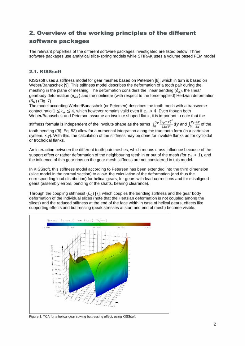
Through the coupling stiffnesst (𝐶𝐶) [7], which couples the bending stiffness and the gear body

deformation of the individual slices (note that the Hertzian deformation is not coupled among the slices) and the reduced stiffness at the end of the face width in case of helical gears, effects like supporting effects and buttressing (peak stresses at start and end of mesh) become visible.

Figure 1: TCA for a helical gear sowing buttressing effect, using KISSsoft

3

2.2. LVR

In the same way as Petersen calculation is based on Weber/Banaschek [9], LVR is also based on this spring-slice model. Compared to KISSsoft however, the slices are not in transverse section but in normal section. As LVR also considers coupled slices, the buttressing effect may also be simulated. LVR does not consider (or this effect is not documented) the cross influence between the different teeth in the mesh.

Figure 2: Helical gear TCA in LVR, showing buttressing effect

2.3. RIKOR

The stiffness model in RIKOR-H [2] partially considers the cross influence. The tooth bending and the tilting in the gear body does not have an influence on the neighbouring teeth, but the effect of torsion

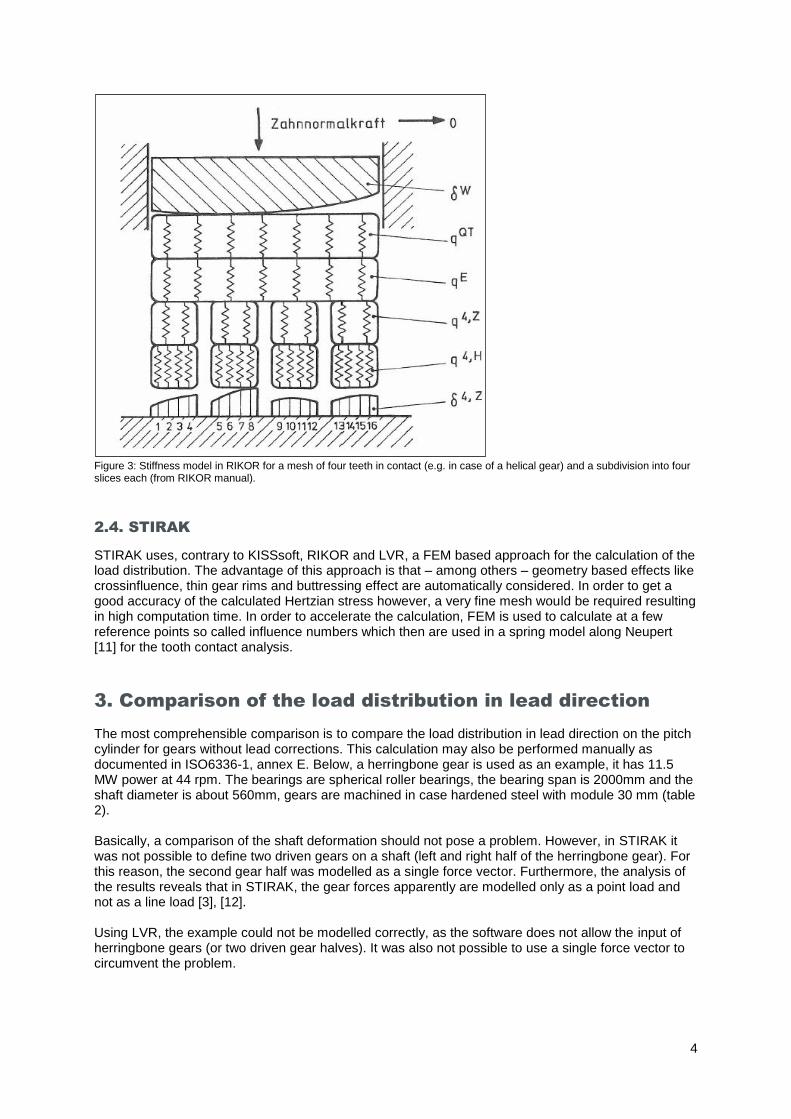
and shear deformation of the gear body (𝑞𝑄𝑇) is considered. The figure describing the model (Figure 3) suggests a full coupling between the individual slices for the

toot deformation (𝑞4,𝑍), tooth tilting (𝑞𝐸), Hertzian deformation (𝑞4,𝐻). But no function for the coupling of the slices is documented. The effect of buttressing cannot be shown or considered in RIKOR H.

4

Figure 3: Stiffness model in RIKOR for a mesh of four teeth in contact (e.g. in case of a helical gear) and a subdivision into four slices each (from RIKOR manual).

2.4. STIRAK

STIRAK uses, contrary to KISSsoft, RIKOR and LVR, a FEM based approach for the calculation of the load distribution. The advantage of this approach is that – among others – geometry based effects like crossinfluence, thin gear rims and buttressing effect are automatically considered. In order to get a good accuracy of the calculated Hertzian stress however, a very fine mesh would be required resulting in high computation time. In order to accelerate the calculation, FEM is used to calculate at a few reference points so called influence numbers which then are used in a spring model along Neupert [11] for the tooth contact analysis.

3. Comparison of the load distribution in lead direction

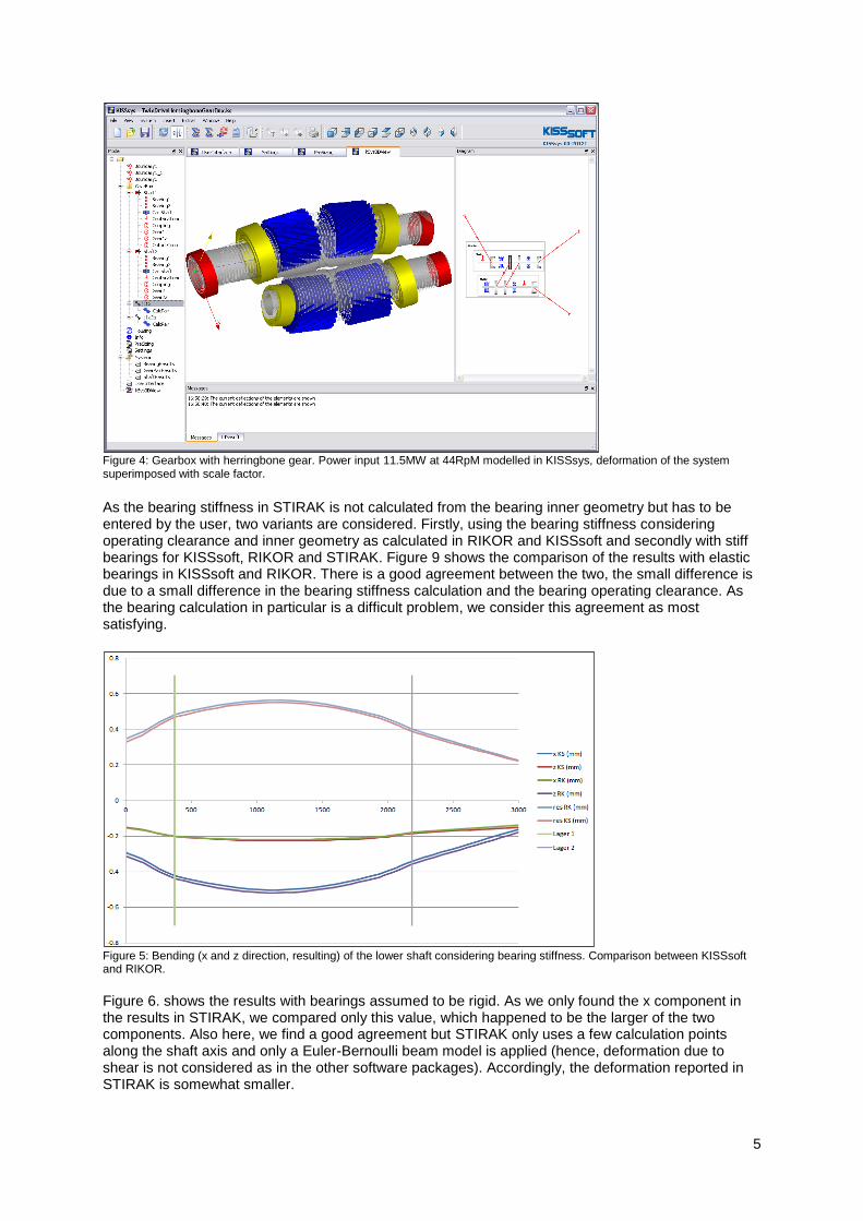
The most comprehensible comparison is to compare the load distribution in lead direction on the pitch cylinder for gears without lead corrections. This calculation may also be performed manually as documented in ISO6336-1, annex E. Below, a herringbone gear is used as an example, it has 11.5 MW power at 44 rpm. The bearings are spherical roller bearings, the bearing span is 2000mm and the shaft diameter is about 560mm, gears are machined in case hardened steel with module 30 mm (table 2). Basically, a comparison of the shaft deformation should not pose a problem. However, in STIRAK it was not possible to define two driven gears on a shaft (left and right half of the herringbone gear). For this reason, the second gear half was modelled as a single force vector. Furthermore, the analysis of the results reveals that in STIRAK, the gear forces apparently are modelled only as a point load and not as a line load [3], [12]. Using LVR, the example could not be modelled correctly, as the software does not allow the input of herringbone gears (or two driven gear halves). It was also not possible to use a single force vector to circumvent the problem.

5

Figure 4: Gearbox with herringbone gear. Power input 11.5MW at 44RpM modelled in KISSsys, deformation of the system superimposed with scale factor.

As the bearing stiffness in STIRAK is not calculated from the bearing inner geometry but has to be entered by the user, two variants are considered. Firstly, using the bearing stiffness considering operating clearance and inner geometry as calculated in RIKOR and KISSsoft and secondly with stiff bearings for KISSsoft, RIKOR and STIRAK. Figure 9 shows the comparison of the results with elastic bearings in KISSsoft and RIKOR. There is a good agreement between the two, the small difference is due to a small difference in the bearing stiffness calculation and the bearing operating clearance. As the bearing calculation in particular is a difficult problem, we consider this agreement as most satisfying.

Figure 5: Bending (x and z direction, resulting) of the lower shaft considering bearing stiffness. Comparison between KISSsoft and RIKOR.

Figure 6. shows the results with bearings assumed to be rigid. As we only found the x component in the results in STIRAK, we compared only this value, which happened to be the larger of the two components. Also here, we find a good agreement but STIRAK only uses a few calculation points along the shaft axis and only a Euler-Bernoulli beam model is applied (hence, deformation due to shear is not considered as in the other software packages). Accordingly, the deformation reported in STIRAK is somewhat smaller.

6

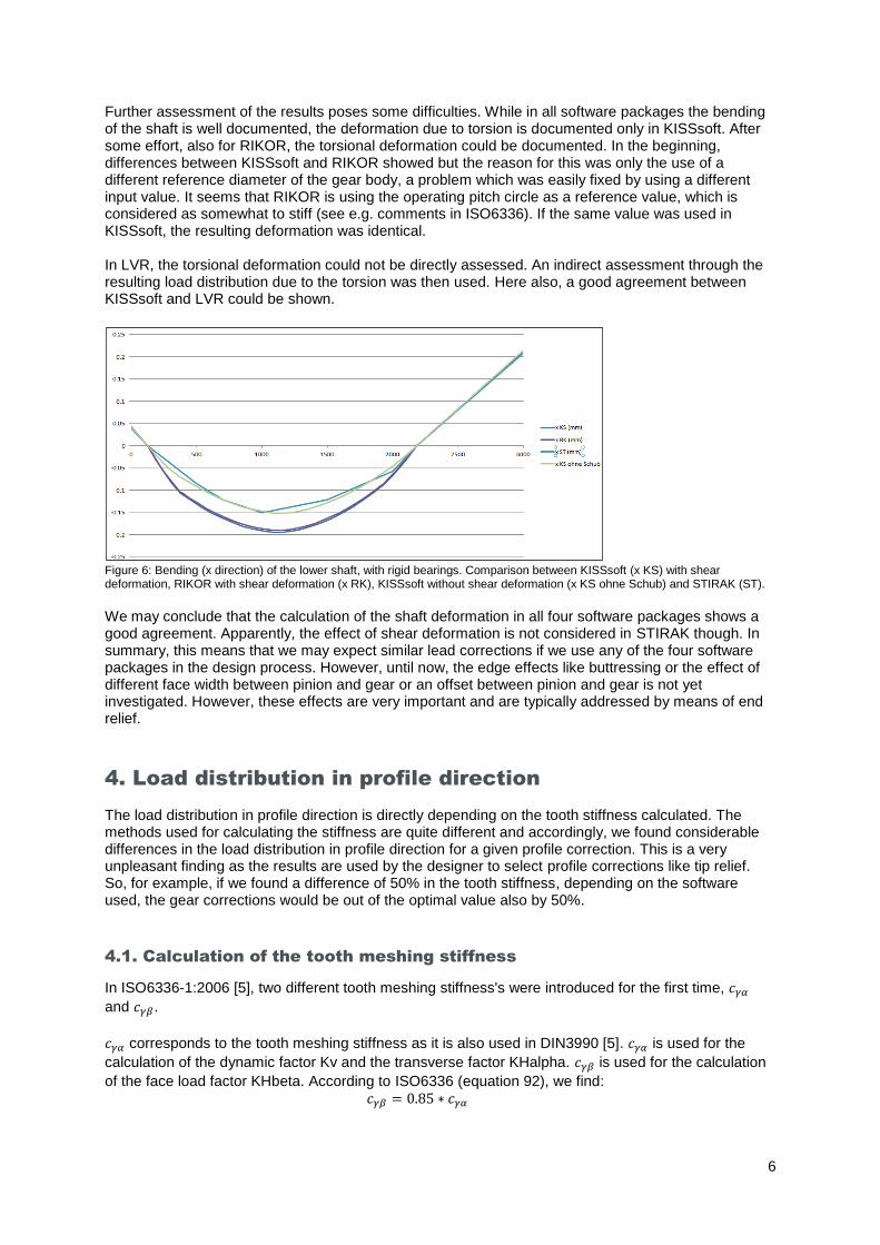
Further assessment of the results poses some difficulties. While in all software packages the bending of the shaft is well documented, the deformation due to torsion is documented only in KISSsoft. After some effort, also for RIKOR, the torsional deformation could be documented. In the beginning, differences between KISSsoft and RIKOR showed but the reason for this was only the use of a different reference diameter of the gear body, a problem which was easily fixed by using a different input value. It seems that RIKOR is using the operating pitch circle as a reference value, which is considered as somewhat to stiff (see e.g. comments in ISO6336). If the same value was used in KISSsoft, the resulting deformation was identical. In LVR, the torsional deformation could not be directly assessed. An indirect assessment through the resulting load distribution due to the torsion was then used. Here also, a good agreement between KISSsoft and LVR could be shown.

Figure 6: Bending (x direction) of the lower shaft, with rigid bearings. Comparison between KISSsoft (x KS) with shear deformation, RIKOR with shear deformation (x RK), KISSsoft without shear deformation (x KS ohne Schub) and STIRAK (ST).

We may conclude that the calculation of the shaft deformation in all four software packages shows a good agreement. Apparently, the effect of shear deformation is not considered in STIRAK though. In summary, this means that we may expect similar lead corrections if we use any of the four software packages in the design process. However, until now, the edge effects like buttressing or the effect of different face width between pinion and gear or an offset between pinion and gear is not yet investigated. However, these effects are very important and are typically addressed by means of end relief.

4. Load distribution in profile direction

The load distribution in profile direction is directly depending on the tooth stiffness calculated. The methods used for calculating the stiffness are quite different and accordingly, we found considerable differences in the load distribution in profile direction for a given profile correction. This is a very unpleasant finding as the results are used by the designer to select profile corrections like tip relief. So, for example, if we found a difference of 50% in the tooth stiffness, depending on the software used, the gear corrections would be out of the optimal value also by 50%.

4.1. Calculation of the tooth meshing stiffness

In ISO6336-1:2006 [5], two different tooth meshing stiffness's were introduced for the first time, 𝑐𝛾𝛼

and 𝑐𝛾𝛽.

𝑐𝛾𝛼 corresponds to the tooth meshing stiffness as it is also used in DIN3990 [5]. 𝑐𝛾𝛼 is used for the

calculation of the dynamic factor Kv and the transverse factor KHalpha. 𝑐𝛾𝛽 is used for the calculation

of the face load factor KHbeta. According to ISO6336 (equation 92), we find: 𝑐𝛾𝛽 = 0.85 ∗ 𝑐𝛾𝛼

7

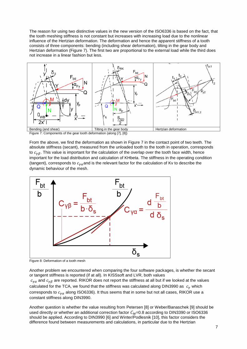
The reason for using two distinctive values in the new version of the ISO6336 is based on the fact, that the tooth meshing stiffness is not constant but increases with increasing load due to the nonlinear influence of the Hertzian deformation. The deformation and hence the apparent stiffness of a tooth consists of three components: bending (including shear deformation), tilting in the gear body and Hertzian deformation (Figure 7). The first two are proportional to the external load while the third does not increase in a linear fashion but less.

Bending (and shear) Tilting in the gear body Hertzian deformation

Figure 7: Components of the gear tooth deformation (along [7], [8])

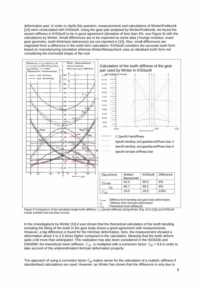
From the above, we find the deformation as shown in Figure 7 in the contact point of two teeth. The absolute stiffness (secant), measured from the unloaded tooth to the tooth in operation, corresponds

to 𝑐𝛾𝛽. This value is important for the calculation of the overlap over the tooth face width, hence

important for the load distribution and calculation of KHbeta. The stiffness in the operating condition

(tangent), corresponds to 𝑐𝛾𝛼and is the relevant factor for the calculation of Kv to describe the

dynamic behaviour of the mesh.

Figure 8: Deformation of a tooth mesh

Another problem we encountered when comparing the four software packages, is whether the secant or tangent stiffness is reported (if at all). In KISSsoft and LVR, both values

𝑐𝛾𝛼 and 𝑐𝛾𝛽 are reported. RIKOR does not report the stiffness at all but if we looked at the values

calculated for the TCA, we found that the stiffness was calculated along DIN3990 as 𝑐𝛾 which

corresponds to 𝑐𝛾𝛼 along ISO6336). It thus seems that in some but not all cases, RIKOR use a

constant stiffness along DIN3990. Another question is whether the value resulting from Petersen [8] or Weber/Banaschek [9] should be

used directly or whether an additional correction factor 𝐶𝑀=0.8 according to DIN3390 or ISO6336 should be applied. According to DIN3990 [6] and Winter/Podlesnik [10], this factor considers the difference found between measurements and calculations, in particular due to the Hertzian

8

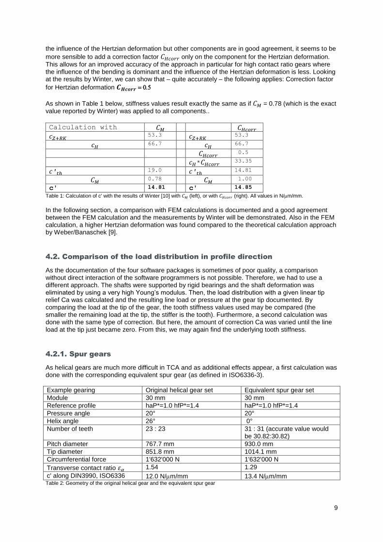
deformation part. In order to clarify this question, measurements and calculations of Winter/Podlesnik [10] were recalculated with KISSsoft. Using the gear pair analysed by Winter/Podlesnik, we found the secant stiffness in KISSsoft to be in good agreement (deviation of less than 5%, see Figure 9) with the calculations by Winter. Small differences are to be expected as some data (Youngs modulus, exact gear geometry, tooth thickness tolerances) are not reported in [10]. Also, small differences are originated from a difference in the tooth form calculation: KISSsoft considers the accurate tooth form based on manufacturing simulation whereas Weber/Banascheck uses an idealised tooth form not considering the trochoidal shape of the root.

Calculation of the tooth stiffness of the gear pair used by Winter in KISSsoft

(N/m/mm) Weber/ Banaschek

KISSsoft Difference

𝑐𝑍+𝑅𝐾 53.3 50.0 6%

𝑐𝐻 66.7 69.2 4%

𝑐′𝑡ℎ 19.0 18.3 3.8%

𝑐𝑍+𝑅𝐾 : Stiffness from bending and gear body deformation 𝑐𝐻 : Stiffness from Hertzian deformation 𝑐′𝑡ℎ : Theoretical mesh stiffness§

Figure 9 Comparison of the calculated single tooth stiffness 𝑐′𝑡ℎ (secant stiffness) along Winter (Fig. 18 in [10]) and KISSsoft results overlaid (red and blue curves).

In the investigations by Winter [10] it was shown that the theoretical calculation of the tooth bending including the tilting of the tooth in the gear body shows a good agreement with measurements. However, a big difference is found for the Hertzian deformation, here, the measurement showed a deformation about 2 to 2.5 times higher compared to the calculation. Meaning that the teeth deform quite a bit more than anticipated. This realisation has also been considered in the ISO6336 and

DIN3990: the theoretical mesh stiffness 𝑐′𝑡ℎ is multiplied with a correction factor 𝐶𝑀 = 0.8 in order to

take account of the underestimated Hertzian deformation properly.

The approach of using a correction factor 𝐶𝑀 makes sense for the calculation of a realistic stiffness if standardised calculations are used. However, as Winter has shown that the difference is only due to

9

the influence of the Hertzian deformation but other components are in good agreement, it seems to be

more sensible to add a correction factor 𝐶𝐻𝑐𝑜𝑟𝑟only on the component for the Hertzian deformation.

This allows for an improved accuracy of the approach in particular for high contact ratio gears where the influence of the bending is dominant and the influence of the Hertzian deformation is less. Looking at the results by Winter, we can show that – quite accurately – the following applies: Correction factor

for Hertzian deformation 𝑪𝑯𝒄𝒐𝒓𝒓

As shown in Table 1 below, stiffness values result exactly the same as if 𝐶𝑀 = 0.78 (which is the exact value reported by Winter) was applied to all components..

Calculation with 𝐶𝑀 𝐶𝐻𝑐𝑜𝑟𝑟

𝑐𝑍+𝑅𝐾 53.3 𝑐𝑍+𝑅𝐾

53.3

𝑐𝐻 66.7 𝑐𝐻

66.7

𝐶𝐻𝑐𝑜𝑟𝑟 0.5

𝑐𝐻*𝐶𝐻𝑐𝑜𝑟𝑟 33.35

𝑐′𝑡ℎ 19.0 𝑐′𝑡ℎ

14.81

𝐶𝑀 0.78 𝐶𝑀

1.00

c' 14.81 c' 14.85

Table 1: Calculation of c' with the results of Winter [10] with 𝐶𝑀 (left), or with 𝐶𝐻𝑐𝑜𝑟𝑟 (right). All values in N/m/mm.

In the following section, a comparison with FEM calculations is documented and a good agreement between the FEM calculation and the measurements by Winter will be demonstrated. Also in the FEM calculation, a higher Hertzian deformation was found compared to the theoretical calculation approach by Weber/Banaschek [9].

4.2. Comparison of the load distribution in profile direction

As the documentation of the four software packages is sometimes of poor quality, a comparison without direct interaction of the software programmers is not possible. Therefore, we had to use a different approach. The shafts were supported by rigid bearings and the shaft deformation was eliminated by using a very high Young’s modulus. Then, the load distribution with a given linear tip relief Ca was calculated and the resulting line load or pressure at the gear tip documented. By comparing the load at the tip of the gear, the tooth stiffness values used may be compared (the smaller the remaining load at the tip, the stiffer is the tooth). Furthermore, a second calculation was done with the same type of correction. But here, the amount of correction Ca was varied until the line load at the tip just became zero. From this, we may again find the underlying tooth stiffness.

4.2.1. Spur gears

As helical gears are much more difficult in TCA and as additional effects appear, a first calculation was done with the corresponding equivalent spur gear (as defined in ISO6336-3).

Example gearing Original helical gear set Equivalent spur gear set

Module 30 mm 30 mm

Reference profile haP*=1.0 hfP*=1.4 haP*=1.0 hfP*=1.4

Pressure angle 20° 20°

Helix angle 26° 0°

Number of teeth 23 : 23 31 : 31 (accurate value would be 30.82:30.82)

Pitch diameter 767.7 mm 930.0 mm

Tip diameter 851.8 mm 1014.1 mm

Circumferential force 1'632'000 N 1'632'000 N

Transverse contact ratio 휀𝛼 1.54 1.29

c' along DIN3990, ISO6336 12.0 N/m/mm 13.4 N/m/mm Table 2: Geometry of the original helical gear and the equivalent spur gear

10

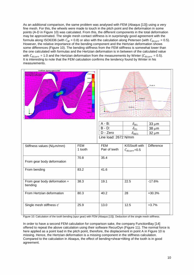
As an additional comparison, the same problem was analysed with FEM (Abaqus [13]) using a very fine mesh. For this, the wheels were made to touch in the pitch point and the deformation in some points (A-D in Figure 10) was calculated. From this, the different components in the total deformation may be approximated. The single mesh contact stiffness is in surprisingly good agreement with the

formula along ISO6336 (with 𝐶𝑀 = 0.8) or also with the calculation along Petersen (with 𝐶𝐻𝑐𝑜𝑟𝑟 = 0.5). However, the relative importance of the bending component and the Hertzian deformation shows some differences (Figure 10). The bending stiffness from the FEM stiffness is somewhat lower than the one calculated with formulas and the Hertzian deformation is in between of the calculated value

with 𝐶𝐻𝑐𝑜𝑟𝑟 = 1.0 and the Hertzian deformation from the measurements by Winter (𝐶𝐻𝑐𝑜𝑟𝑟 = 0.5). It is interesting to note that the FEM calculation confirms the tendency found by Winter in his measurements.

A - B: 𝛿𝐻1 33 m

B - D: 𝛿𝑍1 38 m

D - Zero 𝛿𝑅𝐾1 32 m

Line load: 2672 N/mm

Stiffness values (N/m/mm)

FEM 1 tooth

FEM Pair of teeth

KISSsoft with

𝐶𝐻𝑐𝑜𝑟𝑟=0.5

Difference

From gear body deformation

70.8

35.4

From bending

83.2 41.6

From gear body deformation + bending

38.3 19.1 22.5 -17.6%

From Hertzian deformation

80.3 40.2 28 +30.3%

Single mesh stiffness c'

25.9 13.0 12.5 +3.7%

Figure 10: Calculation of the tooth bending (spur gear) with FEM (Abaqus [13]). Deduction of the single mesh stiffness.

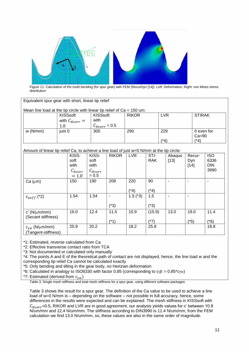
In order to have a second FEM calculation for comparison sake, the company FunctionBay [14] offered to repeat the above calculation using their software RecurDyn (Figure 11). The normal force is here applied as a point load in the pitch point, therefore, the displacement in point A in Figure 10 is missing. Hence, the Hertzian deformation is a missing component in the stiffness calculation. Compared to the calculation in Abaqus, the effect of bending+shear+tilting of the tooth is in good agreement.

11

Figure 11: Calculation of the tooth bending (for spur gear) with FEM (RecurDyn [14]). Left: Deformation, Right: von Mises stress distribution

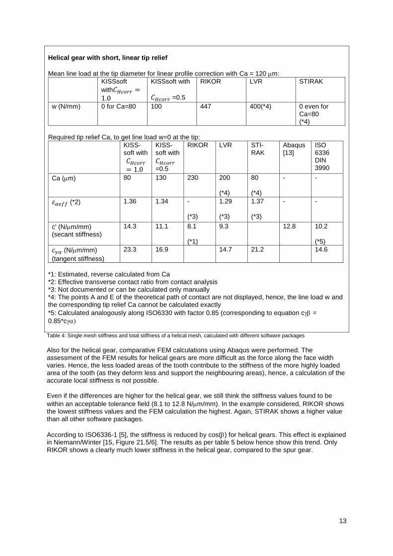
Equivalent spur gear with short, linear tip relief Mean line load at the tip circle with linear tip relief of Ca = 150 um:

KISSsoft

with 𝐶𝐻𝑐𝑜𝑟𝑟 =1.0

KISSsoft with

𝐶𝐻𝑐𝑜𝑟𝑟 = 0.5

RIKOR LVR STIRAK

w (N/mm)

just 0 300 290 229 (*4)

0 even for Ca=90 (*4)

Amount of linear tip relief Ca, to achieve a line load of just w=0 N/mm at the tip circle:

KISS-soft with

𝐶𝐻𝑐𝑜𝑟𝑟

= 1.0

KISS-soft with

𝐶𝐻𝑐𝑜𝑟𝑟

= 0.5

RIKOR LVR STI-RAK

Abaqus [13]

Recur-Dyn [14]

ISO 6336 DIN 3990

Ca (m)

150 190 208 220 (*4)

90 (*4)

- - -

휀𝛼𝑒𝑓𝑓 (*2)

1.54 1.54 - (*3)

1.5 (*3) 1.5 (*3)

- -

c' (N/m/mm) (Secant stiffness)

16.0 12.4 11.5 (*1)

10.9 (15.9) (*7)

13.0 19.0 (*5)

11.4 (*6)

𝑐𝛾𝛼 (N/m/mm)

(Tangent-stiffness)

25.9 20.2 18.2 25.8 18.8

*1: Estimated, reverse calculated from Ca *2: Effective transverse contact ratio from TCA *3: Not documented or calculated only manually *4: The points A and E of the theoretical path of contact are not displayed, hence, the line load w and the corresponding tip relief Ca cannot be calculated exactly *5: Only bending and tilting in the gear body, no Hertzian deformation

*6: Calculated in analogy to ISO6330 with factor 0.85 (corresponding to c = 0.85*c)

*7: Estimated (derived from 𝑐𝛾𝛼)

Table 3: Single mesh stiffness and total mesh stiffness for a spur gear, using different software packages

Table 3 shows the result for a spur gear. The definition of the Ca value to be used to achieve a line load of w=0 N/mm is – depending on the software – not possible in full accuracy, hence, some differences in the results were expected and can be explained. The mesh stiffness in KISSsoft with

𝐶𝐻𝑐𝑜𝑟𝑟=0.5, RIKOR and LVR are in good agreement, our analysis yields values for c‘ between 10.9 N/um/mm and 12.4 N/um/mm. The stiffness according to DIN3990 is 11.4 N/um/mm, from the FEM calculation we find 13.0 N/um/mm, so, these values are also in the same order of magnitude.

12

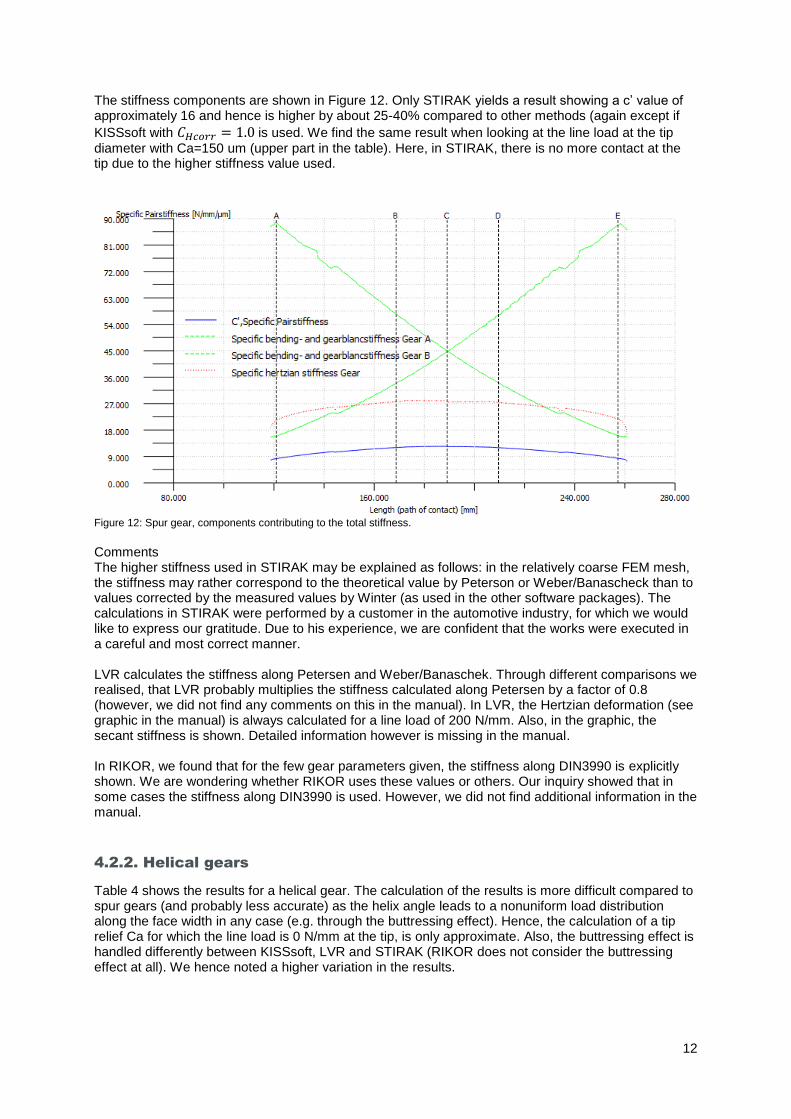
The stiffness components are shown in Figure 12. Only STIRAK yields a result showing a c’ value of approximately 16 and hence is higher by about 25-40% compared to other methods (again except if

KISSsoft with 𝐶𝐻𝑐𝑜𝑟𝑟 = 1.0 is used. We find the same result when looking at the line load at the tip

diameter with Ca=150 um (upper part in the table). Here, in STIRAK, there is no more contact at the tip due to the higher stiffness value used.

Figure 12: Spur gear, components contributing to the total stiffness.

Comments The higher stiffness used in STIRAK may be explained as follows: in the relatively coarse FEM mesh, the stiffness may rather correspond to the theoretical value by Peterson or Weber/Banascheck than to values corrected by the measured values by Winter (as used in the other software packages). The calculations in STIRAK were performed by a customer in the automotive industry, for which we would like to express our gratitude. Due to his experience, we are confident that the works were executed in a careful and most correct manner. LVR calculates the stiffness along Petersen and Weber/Banaschek. Through different comparisons we realised, that LVR probably multiplies the stiffness calculated along Petersen by a factor of 0.8 (however, we did not find any comments on this in the manual). In LVR, the Hertzian deformation (see graphic in the manual) is always calculated for a line load of 200 N/mm. Also, in the graphic, the secant stiffness is shown. Detailed information however is missing in the manual. In RIKOR, we found that for the few gear parameters given, the stiffness along DIN3990 is explicitly shown. We are wondering whether RIKOR uses these values or others. Our inquiry showed that in some cases the stiffness along DIN3990 is used. However, we did not find additional information in the manual.

4.2.2. Helical gears

Table 4 shows the results for a helical gear. The calculation of the results is more difficult compared to spur gears (and probably less accurate) as the helix angle leads to a nonuniform load distribution along the face width in any case (e.g. through the buttressing effect). Hence, the calculation of a tip relief Ca for which the line load is 0 N/mm at the tip, is only approximate. Also, the buttressing effect is handled differently between KISSsoft, LVR and STIRAK (RIKOR does not consider the buttressing effect at all). We hence noted a higher variation in the results.

13

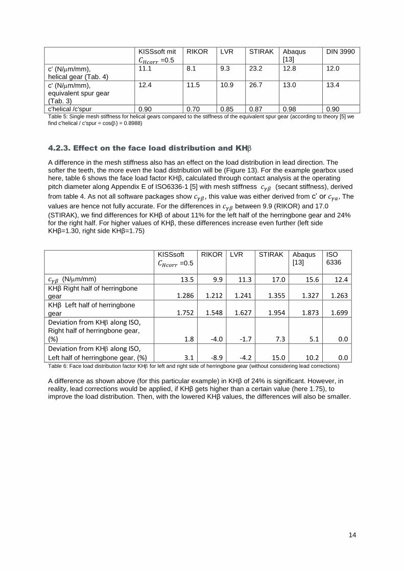
Helical gear with short, linear tip relief

Mean line load at the tip diameter for linear profile correction with Ca = 120 m:

KISSsoft

with𝐶𝐻𝑐𝑜𝑟𝑟 =1.0

KISSsoft with

𝐶𝐻𝑐𝑜𝑟𝑟 =0.5

RIKOR LVR STIRAK

w (N/mm)

0 for Ca=80 100 447 400(*4) 0 even for Ca=80 (*4)

Required tip relief Ca, to get line load w=0 at the tip:

KISS-soft with

𝐶𝐻𝑐𝑜𝑟𝑟

= 1.0

KISS-soft with

𝐶𝐻𝑐𝑜𝑟𝑟

=0.5

RIKOR LVR STI-RAK

Abaqus [13]

ISO 6336 DIN 3990

Ca (m)

80 130 230 200 (*4)

80 (*4)

- -

휀𝛼𝑒𝑓𝑓 (*2)

1.36 1.34 - (*3)

1.29 (*3)

1.37 (*3)

- -

c' (N/m/mm) (secant stiffness)

14.3 11.1 8.1 (*1)

9.3 12.8 10.2 (*5)

𝑐𝛾𝛼 (N/m/mm)

(tangent stiffness)

23.3 16.9 14.7 21.2 14.6

*1: Estimated, reverse calculated from Ca *2: Effective transverse contact ratio from contact analysis *3: Not documented or can be calculated only manually *4: The points A and E of the theoretical path of contact are not displayed, hence, the line load w and the corresponding tip relief Ca cannot be calculated exactly

*5: Calculated analogously along ISO6330 with factor 0.85 (corresponding to equation c =

0.85*c Table 4: Single mesh stiffness and total stiffness of a helical mesh, calculated with different software packages

Also for the helical gear, comparative FEM calculations using Abaqus were performed. The assessment of the FEM results for helical gears are more difficult as the force along the face width varies. Hence, the less loaded areas of the tooth contribute to the stiffness of the more highly loaded area of the tooth (as they deform less and support the neighbouring areas), hence, a calculation of the accurate local stiffness is not possible. Even if the differences are higher for the helical gear, we still think the stiffness values found to be

within an acceptable tolerance field (8.1 to 12.8 N/m/mm). In the example considered, RIKOR shows the lowest stiffness values and the FEM calculation the highest. Again, STIRAK shows a higher value than all other software packages.

According to ISO6336-1 [5], the stiffness is reduced by cos() for helical gears. This effect is explained in Niemann/Winter [15, Figure 21.5/6]. The results as per table 5 below hence show this trend. Only RIKOR shows a clearly much lower stiffness in the helical gear, compared to the spur gear.

14

KISSsoft mit

𝐶𝐻𝑐𝑜𝑟𝑟 =0.5

RIKOR LVR STIRAK Abaqus [13]

DIN 3990

c' (N/m/mm), helical gear (Tab. 4)

11.1 8.1 9.3 23.2 12.8 12.0

c' (N/m/mm), equivalent spur gear (Tab. 3)

12.4 11.5 10.9 26.7 13.0 13.4

c'helical /c'spur 0.90 0.70 0.85 0.87 0.98 0.90 Table 5: Single mesh stiffness for helical gears compared to the stiffness of the equivalent spur gear (according to theory [5] we

find c'helical / c'spur = cos() = 0.8988)

4.2.3. Effect on the face load distribution and KH

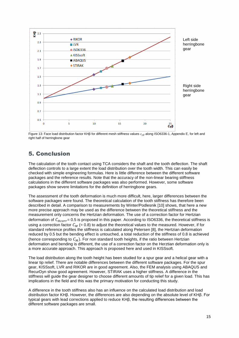
A difference in the mesh stiffness also has an effect on the load distribution in lead direction. The softer the teeth, the more even the load distribution will be (Figure 13). For the example gearbox used here, table 6 shows the face load factor KHβ, calculated through contact analysis at the operating

pitch diameter along Appendix E of ISO6336-1 [5] with mesh stiffness 𝑐𝛾𝛽 (secant stiffness), derived

from table 4. As not all software packages show 𝑐𝛾𝛽, this value was either derived from c’ or 𝑐𝛾𝑎, The

values are hence not fully accurate. For the differences in 𝑐𝛾𝛽 between 9.9 (RIKOR) and 17.0

(STIRAK), we find differences for KHβ of about 11% for the left half of the herringbone gear and 24% for the right half. For higher values of KHβ, these differences increase even further (left side KHβ=1.30, right side KHβ=1.75)

KISSsoft

𝐶𝐻𝑐𝑜𝑟𝑟 =0.5

RIKOR LVR STIRAK Abaqus [13]

ISO 6336

𝑐𝛾𝛽 (N/m/mm) 13.5 9.9 11.3 17.0 15.6 12.4 KHβ Right half of herringbone gear 1.286 1.212 1.241 1.355 1.327 1.263

KHβ Left half of herringbone

gear 1.752 1.548 1.627 1.954 1.873 1.699

Deviation from KH along ISO, Right half of herringbone gear, (%) 1.8 -4.0 -1.7 7.3 5.1 0.0

Deviation from KH along ISO, Left half of herringbone gear, (%) 3.1 -8.9 -4.2 15.0 10.2 0.0 Table 6: Face load distribution factor KH for left and right side of herringbone gear (without considering lead corrections)

A difference as shown above (for this particular example) in KHβ of 24% is significant. However, in reality, lead corrections would be applied, if KHβ gets higher than a certain value (here 1.75), to improve the load distribution. Then, with the lowered KHβ values, the differences will also be smaller.

15

Left side herringbone gear Right side herringbone gear

Figure 13: Face load distribution factor KHβ for different mesh stiffness values 𝑐𝛾𝛽 along ISO6336-1, Appendix E, for left and

right half of herringbone gear

5. Conclusion

The calculation of the tooth contact using TCA considers the shaft and the tooth deflection. The shaft deflection controls to a large extent the load distribution over the tooth width. This can easily be checked with simple engineering formulas. Here is little difference between the different software packages and the reference results. Note that the accuracy of the non-linear bearing stiffness calculations in the different software packages was also performed. However, some software packages show severe limitations for the definition of herringbone gears. The assessment of the tooth deformation is much more difficult, here, larger differences between the software packages were found. The theoretical calculation of the tooth stiffness has therefore been described in detail. A comparison to measurements by Winter/Podlesnik [10] shows, that here a new more precise approach may be used as the difference between the theoretical stiffness and the measurement only concerns the Hertzian deformation. The use of a correction factor for Hertzian

deformation of 𝐶𝐻𝑐𝑜𝑟𝑟= 0.5 is proposed in this paper. According to ISO6336, the theoretical stiffness is

using a correction factor 𝐶𝑀 (= 0.8) to adjust the theoretical values to the measured. However, if for

standard reference profiles the stiffness is calculated along Petersen [8], the Hertzian deformation reduced by 0.5 but the bending effect is untouched, a total reduction of the stiffness of 0.8 is achieved

(hence corresponding to 𝐶𝑀). For non standard tooth heights, if the ratio between Hertzian

deformation and bending is different, the use of a correction factor on the Herztian deformation only is a more accurate approach. This approach is proposed here and used in KISSsoft. The load distribution along the tooth height has been studied for a spur gear and a helical gear with a linear tip relief. There are notable differences between the different software packages. For the spur gear, KISSsoft, LVR and RIKOR are in good agreement. Also, the FEM analysis using ABAQUS and RecurDyn show good agreement. However, STIRAK uses a higher stiffness. A difference in the stiffness will guide the gear designer to choose different amounts of tip relief for a given load. This has implications in the field and this was the primary motivation for conducting this study. A difference in the tooth stiffness also has an influence on the calculated load distribution and load distribution factor KHβ. However, the differences are also depending on the absolute level of KHβ. For typical gears with lead corrections applied to reduce KHβ, the resulting differences between the different software packages are small.

16

For helical gears, similar results are found. Here, the differences are somewhat higher as additional effects like buttressing and stiffening from neighbouring, unloaded areas are added. However, the differences are again considered acceptable. Again, only STIRAK shows higher stiffness values than the other software packages.

6. Literatur

[1] LVR, Software of DriveKonzepts GmbH, Dresden. [2] RIKOR, Software of Forschungsvereinigung Antriebstechnik e.V, Frankfurt. [3] STIRAK, Software of Forschungsvereinigung Antriebstechnik e.V, Frankfurt. [4] KISSsoft, Software of KISSsoft AG, Bubikon, Switzerland. [5] ISO6336, Calculation of load capacity of spur and helical gears, Teil 1-3, 2006. [6] DIN3990, Tragfähigkeitsberechnung von Stirnrädern, Teil 1-3, 1987. [7] B.Mahr, Kontaktanalyse mit KISSsoft, Antriebstechnik 12/2011. [8] D. Petersen: Auswirkung der Lastverteilung auf die Zahnfusstragfähigkeit von hochüberdeckenden Stirnradpaarungen, Fakultät Maschinenbau, TU Braunschweig, 1989. [9] Weber, C.; Banaschek, K.; Formänderung und Profilrücknahme bei gerade- und schrägverzahnten Stirnrädern. Schriftenreihe Antriebstechnik Nr.11, Verlag Vieweg, Braunschweig (1953). [10] Winter, H.; Podlesnik, B.; Zahnfedersteifigkeit von Stirnradpaaren, Teile 1, 2 und 3; Antriebstechnik Nr. 22 (1983) und Nr. 23(1984). [11] Neupert, B. Berechnung der Zahnkräfte, Pressung und Spannungen von Stirn- und Kegelradgetrieben, RWTH Aachen, 1983 [12] Falk, S. Die Berechnung des beliebig gestützten Durchlauftägers nach dem Reduktionsverfahren, Ingenieur-Archiv, 1956 [13] R. Stebler, Berechnung mit ABAQUS, 2012, Matzendorf. [14] RecurDyn, Simulationsprogramm der FunctionBay GmbH, München. [15] Niemann G., Winter H.: Maschinenelemente, Band 2. Springer Verlag Berlin, 1983