Embed Size (px)
Citation preview

Edith Cowan University Edith Cowan University
Research Online Research Online
Theses : Honours Theses
2010
Comparison and application of three decorrelation methods PCA, Comparison and application of three decorrelation methods PCA,
MAF and ACDC MAF and ACDC
Jacqueline Ferreira Edith Cowan University
Follow this and additional works at: https://ro.ecu.edu.au/theses_hons
Part of the Statistical Methodology Commons
Recommended Citation Recommended Citation Ferreira, J. (2010). Comparison and application of three decorrelation methods PCA, MAF and ACDC. https://ro.ecu.edu.au/theses_hons/1217
This Thesis is posted at Research Online. https://ro.ecu.edu.au/theses_hons/1217

Edith Cowan University
Copyright Warning
You may print or download ONE copy of this document for the purpose
of your own research or study.
The University does not authorize you to copy, communicate or
otherwise make available electronically to any other person any
copyright material contained on this site.
You are reminded of the following:
Copyright owners are entitled to take legal action against persons who infringe their copyright.
A reproduction of material that is protected by copyright may be a
copyright infringement. Where the reproduction of such material is
done without attribution of authorship, with false attribution of
authorship or the authorship is treated in a derogatory manner,
this may be a breach of the author’s moral rights contained in Part
IX of the Copyright Act 1968 (Cth).
Courts have the power to impose a wide range of civil and criminal
sanctions for infringement of copyright, infringement of moral
rights and other offences under the Copyright Act 1968 (Cth).
Higher penalties may apply, and higher damages may be awarded,
for offences and infringements involving the conversion of material
into digital or electronic form.
THE COMPARISON AND APPLICATION OF THREE DECORRELATION METHODS PCA, MAF AND
ACDC.
BY
JACQUELINE FERREIRA
A Thesis Submitted to the
Faculty of Computing, Health and Science
Edith Cowan University
Perth, Western Australia
In Partial Fulfilment of the Requirements for the Degree of
Bachelor Science Honours (Mathematics)
January 2010
Supervisors: Associate Professor Ute Mueller
Dr Steven Richardson

USE OF THESIS
The Use of Thesis statement is not included in this version of the thesis.

Abstract
Geostatistics is a branch of applied mathematics that deals with spatially correlated data.
Analysing and modelling spatially correlated data can be difficult and time consuming,
especially for a multivariate data set. One of the techniques used to make analysis and
modelling easier involves decorrelation, whereby a linear transformation on the sample
variables is used to associate the spatially correlated variables with a set of decorrelated
factors which are statistically and spatially independent. PCA was one of the first
multivariate techniques and is mostly used as a data reduction technique. A popular
alternative decorrelation technique often used in the mining industry is MAF. A study
conducted by Bandarian (2008) found a relatively new decorrelation technique known
as ACDC to be the method which produced the best spatial decorrelation for a
multivariate moderately correlated data set consisting of four variables.
In this thesis the PCA, MAF and ACDC methods are described and then applied to a
multivariate data set supplied by Rio Tinto's Iron Ore Operations. Secondly, we explore
whether it is preferable for the data set to be standardised or transformed via Gaussian
anamorphosis to normal scores before being decorrelated.
The data set consists of ten variables; however the three decorrelation methods were
only applied to a subset of five variables (Fe, Ah03, Si02, LOI and Ti02) which have
the greatest similarity from a statistical and spatial point of view. The three methods
were applied to both standardised and normalised data. For ACDC, additional inputs
such as weights, number of iterations, tolerance and an initial guess for the
diagonalising matrix were explored and investigated in order to get the best spatial
decorrelation results possible.
The overall best spatial decorrelation was achieved by performing ACDC on the
standardised variables, using the matrix of eigenvectors of the correlation matrix as the
initial guess for the diagonalising matrix as well as the first four experimental
semivariogram matrices in the decorrelation. Transforming the variables to normal
scores before decorrelation was found to be of no benefit, as the factors that were
derived from the normalised variables with the exception of one, were not normally
distributed following the decorrelation.
Ill

Copyright and Access Declaration
I certify that this thesis does not, to the best of my knowledge and belief:
(i) Incorporate without acknowledgment any material previously submitted for a
degree or diploma in any institution of higher education;
(ii) Contain any material previously published or written by another person except
where due reference is made in the text; or
(iii) Contain any defamatory material.
(iv) Contain any data that has not been collected in a manner consistent with ethics approval.
The Ethics Committee may refer any incidents involving requests for ethics approval
after data collection to the relevant Faculty for action
Signed ...................... .
.Qd.- \~.;zo\o Dated ............................................................................................... .
IV

Acknowledgement
I would like to thank RioTinto Iron Ore Operations for making the Iron Ore multivariate
data set available to me. I would like to thank Dr Steven Richardson for his patience,
motivation, enthusiasm and positive attitude throughout this thesis. I would especially
like to thank Associate Professor Ute Mueller for her patience, guidance, support,
knowledge and encouragement throughtout my studies at Edith Cowan University;
without her this thesis would not be possible.
To my wonderful family, Mom, Dad and sisters, Dominique and Jeanette, I would like
to thank them all so very much for their ongoing support, words of encouragement,
patience and most importantly for always believing in me. Thank you for always being
there and trying to make my life that little bit easier during my time of study. To my
close friend Monica and her family I would like to thank them for their ongoing
enthusiasm and support throughout my studies. Finally, thanks must go to my special
dogs, Romeo and Bonita, for always brightening up my days.
v

VI

Table of Contents
1. Introduction ....................................................................................................... 1
1.1 Background and Significance ......................................................................... 1
1.2 Aims and Objectives ....................................................................................... 3
1.3 Thesis Outline ................................................................................................. 4
1.4 Software ........................................................................................................... 4
1.5 Notation ........................................................................................................... 5
1.6 Acronyms and Abbreviations .......................................................................... 8
2 Theoretical Framework ...................................................................................... 9
2.1 Multivariate Random Function ....................................................................... 9
2.2 Experimental Measures of Bivariate Relations ............................................. 11
2.3 Linear Model of Co-regionalisation .............................................................. 13
2.4 Linear Transformation Methods ................................................................... 14
2.4.1 PCA ............................................................................................................ 14
2.4.2 MAF ........................................................................................................... 15
2.4.3 ACDC ......................................................................................................... 17
2.5 Methods Used to Assess Spatial Decorrelation ............................................ 21
3 Analysis ............................................................................................................ 23
3.1 Data Set Background.; ................................................................................... 23
3.2 Exploratory Data Analysis ............................................................................ 24
3.3 Spatial Analysis ............................................................................................. 29
3.4 Transforming the Data Set ............................................................................ 31
3.5 Subsets .......................................................................................................... 33
3.6 Linearity ........................................................................................................ 35
3.7 Analysis of Experimental Semivariograms ................................................... 38
Chapter 4 Results ................................................................................................ 39
4.1 Decorrelation Results .................................................................................... 39
4.1.1 PCA Decorrelation Results ........................................................................ 39
4.1.2 MAF Decorrelation Results ....................................................................... 43
4.1.3 ACDC Decorrelation Results ..................................................................... 46
VII

4.2 Comparison of Results .................................................................................. 55
5. Discussion and Conclusion ............................................................................. 59
Reference .......................................................................... , ................................. 63
Appendices .......................................................................................................... 65
Appendix 1 - Standardised Variables ................................................................. 66
Appendix 2- Normal Scores ................................................................................ 67
2.1 Ananmorphosis Parameters Files .................................................................. 68
Appendix 3 -Average Distances, Experimental Semivariogram Matrices and
Eigenvalues ......................................................................................................... 78
Appendix 4- Scatter Plots and Correlation Coefficients of Factors .................. 84
4.1 PCA Factors using Normal Scores ................................................................ 84
4.2 PCA Factors using Standardised Variables .................................................. 85
4.3 MAF Factors using Normal Scores ............................................... , ............... 86
4.4 MAF Factors using Standardised Variables .................................................. 87
4.5 ACDC Factors using Normal Scores ............................................................ 88
4.6 ACDC Factors using Standardised Variables ............................................... 89
4. 7 ACDC Factors using Normal Scores and Matrix AoNs ................................. 90
4.8 ACDC Factors using Standardised Variables and Matrix A05t .................... 91
Appendix 5- Experimental Cross Semivariograms and Spatial Decorrelation
Plots of the ACDC Factors .................................................................................. 92
Appendix 6- MATLAB CODES ..................................................................... 112
6.1 ACDC code ................................................................................................. 112
6.2 Spatial Decorrelation Code Using ACDC method ..................................... 116
6.3 Spatial Decorrelation Code Using MAF and PCA Factors ......................... 121
VIII

List of Figures
Figure 1-The histograms for each of the ten variables, in alphabetical order ................. 25
Figure 2- The qqplots for each of the ten variables, in alphabetical order ..................... 26
Figure 3-Base map for study region ................................................................................ 27
Figure 4- The spatial maps for each of the ten variables in alphabetical order .............. 28
Figure 5- The spatial maps for each ofthe ten variables in alphabetical order .............. 30
Figure 6-Gaussian anamorphosis for each ofthe ten variables in alphabetical order ..... 32
Figure 7- The scree plot (left) and correlation circle (right) ........................................... 33
Figure 8- The scatter plots and correlation coefficients between each of the five
transformed normal score variables in the subset. .......................................................... 36
Figure 9- The scatter plots and correlation coefficients between each of the five
standardised variables in the subset. ............................................................................... 3 7
Figure 10- The experimental cross semivariograms ofthe five normal scores (left) and
standardised (right) variables .......................................................................................... 38
Figure 11- The experimental direct semivariograms of the five normal scores (left) and
standardised (right) variables .......................................................................................... 38
Figure 12- The histograms of the PCA factors using the normal scores subset. ........... .41
Figure 13- The histograms of the PCA factors using the standardised subset. .............. .42
Figure 14- The histograms of the MAF factors using the normal scores subset.. .......... .44
Figure 15- The histograms of the MAF factors using the standardised subset.. ............ .45
Figure 16- The histograms of the ACDC factors using the normal scores subset and first
eleven experimental semivariogram matrices ................................................................. 48
Figure 17- The histograms of the ACDC factors using the standardised subset. ........... 50
Figure 18- The histograms of the ACDC factors using the normal scores subset, the
matrix AoNs and first nine experimental semivariogram matrices .................................. 53
Figure 19- The histograms of the ACDC factors using the standardised subset and the
matrix A0 st ...................................................................................................................... 55
Figure 20- The plots of all the average spatial decorrelation results. The x axes title
'Number of Zeros' represent the number of zeros present in the weight vector ............. 55
Figure 21- The experimental cross semivariograms of the factors obtained for each of
the methods ..................................................................................................................... 57
Figure 22- The plots of the spatial decorrelation (((h), r(h) and K(h)) for every lag
for all the factors ............................................................................................................. 58
IX

List of Tables
Table 1- Summary statistic for the ten variables ............................................................. 24 Table 2- Correlation co-efficient matrix between the ten variables. The highlighted cells represent a correlation coefficient higher than 0.7 .......................................................... 27 Table 3- Minimum, maximum and number of polynomials used for each Gaussian anamorphosis fit. ............................................................................................................. 31 Table 4- Factor pattern matrix for the two factors .......................................................... 34 Table 5- The correlation coefficients for the five transformed normal scores ................ 35 Table 6- The correlation coefficients for the five standardised variables ....................... 35 Table 7- The Kolmogorov-Smimov statistics test of normality results for all the PCA factors using the normal scores subset. ........................................................................... 41 Table 8-The PCA average spatial decorrelation measures using both the normal scores and standardised subset. .................................................................................................. 43 Table 9- The Kolmogorov-Smimov statistics test of normality results for all the MAF factors using the normal scores subset ............................... ~ ............................................ 45 Table 10- The MAF average spatial decorrelation measures using both the normal score subset and standardised subset. ....................................................................................... 45 Table 11- The ACDC weights and corresponding average spatial decorrelation values using the normal scores subset. The borders indicate the best spatial decorrelation values for that column ..................................................................................................... 4 7 Table 12- The Kolmogorov-Smimov statistics test ofnormalityresults for all the ACDC factors using the normal scores subset and first eleven experimental semivariogram matrices ........................................................................................................................... 48 Table 13- The ACDC weights and corresponding average assessment values using the standardised subset. The borders indicate the best spatial decorrelation values for that column ............................................................................................................................. 49 Table 14- The ACDC weights and corresponding average assessment values using the normal scores subset and the matrix AoNs. The borders indicate the best spatial decorrelation values for that column ............................................................................... 52 Table 15- The Kolmogorov-Smimov statistics test ofnormalityresults for all the ACDC factors using the normal scores subset, the matrix AoNs and first nine experimental semivariogram matrices .................................................................................................. 53 Table 16- The ACDC weights and corresponding average assessment values using the standardised subset, the matrix A08t and first four experimental semivariogram matrices. The borders indicate the best spatial decorrelation values for that column .................... 54
X

1 .. Introduction
1.1 Background and Significance
Geostatistics is a branch of applied mathematics that deals with spatially correlated data.
It originated in the early fifties in the mining industry, to help solve ore reserve
estimation problems. The techniques used have evolved over time and are currently
being used in areas such as petroleum geology, hydrogeology, hydrology, meteorology,
oceanography, human geography, forestry, environmental control, landscape ecology
and even epidemiology (Wackemagel, 2003). The main aim of geostatistics is to
analyse, interpret, and derive a model from a sampled data set which may be spatially
correlated in a study region, to provide accurate and reliable estimates of variables at
unsampled locations. It is common that for each location under consideration there are
several variables that may have to be analysed jointly.
There are a variety of multivariate geostatistical techniques used today, making analysis
and modelling of several spatially correlated variables across a study region much
easier. One of these techniques involves decorrelation, whereby a linear transformation
of the sample variables is used to associate the spatially correlated variables with a set
of decorrelated factors which are statistically and spatially independent. Univariate
geostatistical techniques can then be used to model and possibly simulate the
uncorrelated factors, decreasing the complexity and shortcomings of multivariate
techniques, such as decreasing the size of cokriging systems used in multivariate
estimations or simulations.
Principal component analysis (PCA) was one of the first multivariate techniques and is
mostly used as a data reduction technique. Here the aim is to reduce a data set with a
large number ofvariables to a smaller subset ofuncorrelated factors, which accounts for
a large proportion of the variability in the original variables. PCA is based on the
eigenvector-eigenvalue decomposition of either the variance-covariance matrix or
correlation matrix between variables (Desbarats & Dimitrakopoulos, 2000). However,
the problem with PCA is that it only successfully decorrelates the factors at a lag
spacing of zero. The factors will only be uncorrelated for all lags, other than zero, in the
case of intrinsic correlation (Wackemagel, 2003). Most data sets do not exhibit intrinsic
1

correlation and therefore the PCA method is very limited and often does not provide the
best decorrelation results.
The method of minimum/maximum autocorrelation factors (MAF) is another linear
transformation technique based on PCA that decorrelates a set of variables into
uncorrelated factors for all lag spacings, provided that the covariance function of the
variables is characterised by a model of coregionalisation which consists of two
structures to ensure orthogonality for all lag spacings. MAF was first developed by
Switzer and Green (1984) as a data based approach used for multivariate spatial
imaging. It was later shown by Desbarats and Dimitrakopoulos (2000) to be suitable for
decorrelating variables in geostatical real data sets by applying the method to simulate a
regionalised pore size distribution. The computational properties of MAF and
limitations concerning a geostatistical context were later discussed by Vargas-Guzman
and Dimitrakopoulos (2003) who also discuss extending the MAF approach to three
covariance structures, but conclude that this is in general impossible. The method's
current assumption of a two structure linear model of coregionalisation (2SLMC) can be
restrictive as the model of a nugget plus one structure or two structures may be
inadequate to model all spatial features (Bandarian, 2008). A recent study by Rondon
and Tran (2008) in which the MAF method was used on a number of different data sets
showing weak or non-linear correlations, also discusses a number of limitations and
difficulties that may occur using the MAF method. A more general approach for spatial
decorrelation is to approximately diagonalise a set of target matrices which originate
from the experimental semivariogram matrices calculated at all relevant lag spacings.
One of the methods which can be used to do so is the Alternating Columns and
Diagonal Centres method, or more commonly known by its acronym ACDC. The
ACDC method is a joint approximate diagonalisation (JAD) method. The ACDC
method was first proposed by Y eredor in 2000 and is a relatively new linear
transformation method. The ACDC method differs from the other JAD methods as it is
not restricted to only finding an orthogonal diagonalising matrix (Yeredor, 2000).
A study performed by Bandarian (2008) illustrated and compared a variety of linear
transformation methods using a subset of the Jura data set (Goovaerts, 1997), two of the
methods which were considered where the MAF and ACDC. The subset consisted of
four moderately correlated variables (Cd, Co, Cr and Ni). The results found the ACDC
method to produce the better spatial decorrelation for the multivariate Jura subset,
2

thereby rmsmg the question whether the ACDC method is the better linear
transformation method to decorrelate any multivariate data set.
The linear transformation method, MAF (minimum/ maximum autocorrelation factors)
is currently used in the mining industry to reduce complexity and time devoted to
analysing and modelling multivariate data sets·. Mining companies are often looking for
the most cost effective methods which produce the best results. With this in mind even
though most linear transformation methods only approximately diagonalise a
multivariate data set, it would be cost effective to use the linear transformation method,
whether it be ACDC or MAF, which produces the best spatial decorrelation, taking into
account the time involved in using the linear transformation methods.
1.2 Aims and Objectives
The ultimate aim of this study is to compare the ACDC and MAF methods and
determine if the ACDC method is able to approximately decorrelate a multivariate data
set of more than four variables better than the currently used MAF method. Both
methods will be applied to a multivariate data set from a channel iron ore deposit
supplied by Rio Tinto's Iron Ore Operations. The factors obtained from both methods
will be examined in order to determine which decorrelation method produces the best
spatial decorrelation. Some of the variables in the data set are highly correlated. The
effectiveness of both of the methods on the highly correlated data will also be
considered.
The multivariate data set supplied by Rio Tinto consists of ten variables. A subset
grouping all the variables which are statistically and spatially similar will be discussed
in order to avoid variables which may be problematic. The most important variables are
aluminium oxide, iron and silica which will need to be modelled jointly and hence have
to be included in the subset, while there are other variables which may not be
appropriate to add to the subset due to geological reasons. This will be discussed further
in the thesis. Therefore, a suitable subset needs to be explored.
The ACDC algorithm, implemented in Matlab, allows for a variety of additional inputs
besides the target matrices which could potentially affect the decorrelation results. The
additional inputs such as weights, number of iterations, tolerance and an initial guess for
the diagonalising matrix will be explored and investigated in order to get the best spatial
decorrelation results possible using the ACDC method.
3

The decision to standardise the data set or to normalise the data before applying the
methods is another interesting aspect which will be explored. This simple decision may
have an effect on the decorrelation results for either method.
1.3 Thesis Outline
This thesis consists of five chapters and an Appendix. Chapter 2 discusses the
theoretical framework significant to this study. This includes the multivariate random
function model, linear model of co-regionalisation, a discussion of the linear
transformation methods and finally how the spatial decorrelation will be assessed.
Chapter 3 gives background information about the variables in the multivariate data set
as well as a detailed exploratory data analysis of the data. The last few sections of
Chapter 3 consist of the transformations of the variables and the investigation into
suitable subsets. The results of the spatial decorrelation for all the methods are given in
Chapter 4. The final chapter involves the discussion and conclusion.
1.4 Software
The main software packages used are Isatis and Matlab. Isatis is a geostastics software
package which was mainly used to carry out exploratory data analysis, spatial data
analysis and calculation of experimental semivariograms. The Gaussian anamorphosis
function in Isatis was used to transform the original data to normally distributed data.
The variables were also standardised using the corresponding population means and
standard deviations calculated in Isatis. The MAF technique in Isatis was used to
calculate the factors which were then analysed in Isatis. All the factors produced from
ACDC, MAF and PCA were analysed in Isatis and SPSS.
Matlab is an engineering/mathematical software package in which the ACDC algorithm
has been coded by Yeredor (2004). The target matrices produced in Isatis are run
through the ACDC algorithm in Matlab to produce a transformation matrix that will
approximately diagonalise the data. Matlab was furthermore used to calculate the spatial
decorrelation assessment results for all the factors as well as the graphs showing the
results. Microsoft Word and Excel were used for presentation and data preparation
purposes. Finally SPSS was used to investigate the relationship between the variables.
4

1.5 Notation
The majority of the notation used in this thesis comes from Goovaerts (1997).
A:
a:
bl . ij .
study region
maximum range of the semivariogram
ACDC transformation matrix
initial diagonalising matrix
coefficients of the basic semivariogram model Bl (h) in the linear
model of co-regionalisation
Bl : co-regionalisation matrix containing the coefficients bfj of the
semivariogram model Bl (h) in the corresponding linear model of co
regionalisation
B: matrix of correlation coefficient
C(O): covariance value at separation distance lhi=O
C(h): covariance function of the random function for lag vector h
C(h): experimental covariance function matrix of size K X K
Cij(h): experimental cross covariance between the two random function Zi and
Zj for a lag vector h
C18 (·): objective function
D: diagonal matrix
£{·}: expected values
F(u): factor values
f(h): semivariogram matrix of size K x K
f(·): experimental semivariogram matrix of size K x K
Bl (h): lth basic semivariogram model in the linear model of co-regionalisation
5

Yij(h): experimental cross semivariogram between Zi and Zj at lag value h
Yij(h): cross semivariogram between Zi and Zj at lag value h
h: separation vector
] : number of lag spacings
K(h): spatial diagonalisation efficiency at lag h.
K". average diagonalisation efficiency for all lags.
K: number ofvariables
A: eigenvalue matrix
A.: eigenvalue
L: number of models required to capture the spatial continuity of the
attributes
m: lagmeans
subscript NS: normal scores data set
n: number of samples in the study region A
N (h): is the number of pairs of data locations separated by the vector h
Q: PCA eigenvector matrix
pij: experimental correlation coefficient between zi and Zj
Pij(h): cross correlogram between zi and Zj for the lag vector h
8ij: experimental covariance between zi and Zj
CJ2
: lag variance
subscript St: standardised data set
r(h): quotient of the absolute deviation from diagonality and the sum of the
factor main diagonal entries efficiency at lag h.
6

f: the average quotient of the absolute deviation from diagonality and the
sum of the factor main diagonal entries efficiency for all lags.
Tr { ·}: trace of a matrix
u: coordinate vector
Ua: datum location
<;(h): the measure of absolute deviation from diagonality for each lag h
~: the average measure of absolute deviation from diagonality for all lags
wi: . weight vector
X: MAF eigenvector matrix
XT: MAF transformation matrix
Z: multivariate random valued function
zi(ua): zrdatum values at location Ua
zi(u): zi-datum values at location u
z(u): vector of true values of K attributes at location u
z(u): true value at unsampled location u
Z(u): vector of continuous random variable at location u
Zi(u): ith continuous random variable at location u
7

1.6 Acronyms and Abbreviations
The acronyms and abbreviations listed below are used in the content, Figure and Tables
throughout the thesis.
ACDC: Alternative Columns and Diagonal Centres method
Aluminium oxide
Calcium oxide
Fe: Iron
JAD: Joint Approximate Diagonalisation
LOI: Loss on Ignition or The measurement of water content of the ore
MAF: Maximum/minimum autocorrelation factors
MgO: Magnesium oxide
Mn: Manganese
P: Phosphorus
PCA: Principle component analysis
S: Sulphur
Silicon dioxide or silica
Titanium dioxide or Titania
2SLMC: Two structure linear model of coregionalisation
8

2 Theoretical Framework In this chapter we discuss the theoretical framework appropriate for this study. The first
part includes the geostatistical concepts relevant to the study, while the second part
includes information about the linear model of co-regionalisation. The three linear
transformation methods, PCA, MAF and ACDC, will also be discussed in this chapter
along with the way in which the spatial decorrelation for each method will be assessed.
2.1 Multivariate Random Function
Geostatistics is based upon the concept of the random function, whereby a set of
unknown values are regarded as realisations of spatially dependent random variables. A
sample on a study region, A, consists of a set of measurements at specific locations for a
number of attributes. The measurements in this region can be defined as
{ zi(ua), Ua E A, a=l, ... , n, i=l, .. . , K},
where Ua is the ath sampled location for n samples and zi is defined as the lh attribute
of K attributes. The set of values the variable zi attains on the study region A is
defined as
The value zi(u) can be thought of as being a realisation of the corresponding random
variable Zi(u) at the location u inA. When we consider the study region as a whole,
we have a set of usually dependent random variables, and can define a function from the
study region A to the set {Zi(u): u E A}, known as a random function.
In the multivariate case the vector, z(u) = [z1 (u), ..... , zK(u)Y of K attributes at
location u can be viewed as a realisation of the random variable valued vector Z(u) =
[Z1 (u), ..... ,ZK(u)f. The multivariate random function can therefore be defined as
Z: A~ {[Z1 (u), .... , ZK(u)]: u E A}.
Several assumptions need to be made about the multivariate random function. A random
function is called stationary if for any separation vector h, the joint distributions of
[Z(u1),Z(u2 ) ..... ,Z(uk)] and [Z(u1 + h),Z(u2 +h) ..... ,Z(uk +h)] are identical
for any lag h and for any k. The assumption of stationarity is impo-ssible to test and so
9

the weaker assumption of second order stationarity is used in practice. A random
function is said to be second order stationary if the expected mean value
m= E{Z(u)},
exists and is invariant within A. Herem= [m1 (u), ..... , m~u)JT and£{·} denotes the
mathematical expectation. The covariance function
C(h) = E{[Z(u)- m] · [Z(u +h)- m]T}
only depends on the separation vector h. The covariance function must be a positive
definite function. In many cases the assumption of second-order stationarity is not met
and a weaker hypothesis, second order stationarity of the increments Z(u)- Z(u +h)
is assumed. When the increments are second-order stationary, the random function is
said to be intrinsic stationary. In this case the mean
E{Z(u +h)- Z(u)}
exists and is equal to 0 and the semivariogram
f(h) = ~ E {[Z(u)- Z(u +h)]· [Z(u)- Z(u + h)]T} 2
depends only on h. The semivariogram matrix, f(h), is a K x K positive definite,
symmetric matrix that contains the direct semivariograms results along the main
diagonal and the experimental cross semivariogram off the diagonal. When the
variance-covariance matrix C(O) exists, the semivariogram matrix and covariance
function matrix are related by
f(h) = C(O)- C(h).
The semivariogram function is more commonly used in practise than the covariance
function.
10

2.2 Experimental Measures of Bivariate Relations
The covariance and correlation coefficient are the most frequently used measures of
bivariate relations. The experimental covariance Bij is a measure of the joint variation of
zi and Zj around their means and it is computed as
n
Bij = ~ I (zi(a)- ma . (zj(a)- mj), a=1
where the arithmetic means of zi and zj are denoted by mi and mj, respectively. In the
situation when i = j the covariance becomes the variance.
The standardised form of the experimental covariance IS the linear correlation
coefficient Pij which provides a measure of the linear relationship between two
variables. The experimental correlation coefficient is calculated as
(J·.
~ lJ E[-1,1] Pij = CJ· . CJ·
l 1
where CJi and CJj are the standard deviations of zi and Zj, respectively. The correlation
matrix B is a matrix of correlation coefficients Pij for all pairs i,j = 1 .... K. When the
variables have been transformed to normal scores or standardised the correlation matrix
is equivalent to the covariance matrix.
Spatial features of the data such as the location of extreme values, degree of continuity
and spatial trends are often of considerable interest in geostatistics, and there are a
variety of tools used to capture spatial continuity. In a multivariate data set consisting of
several attributes, such as the data set that will be used for this project, there is a need to
look at spatial cross continuity between measurements of different attributes. The cross
covariance and cross correlation function are some of the measures of spatial continuity
derived from the sample data that measure the similarities between colocated data. The
experimental cross covariance function is the covariance between a pair of locations of
different attributes, zi and Zj, separated by a vector h, which is also known as the lag.
The experimental cross covariance function is defined as
11

with
N(h) N(h)
mLh = N~h) I zi(ua) 1 and a=1
mj +h = N~h) I Zj(Ua +h) 1
a=1
where N(h) is the number of pairs of data locations separated by the vector h, while
mLh and mj +h are the means of the zi and Zj values. When i=j this is simply lrnown as
the experimental covariance function between data values of the same attribute
separated by a vector h. The cross correlogram is the standardised form of the
covariance and is given by
E [-111] (]'.2 (Jf
t -h 1 +h
with
where a? -h and af +h are the variances of zi and zj values. In the case where i=j the
function is known as a correlogram and measures the similarities between data of the
same attribute.
The experimental cross semivariogram 1s another measure of spatial continuity,
however unlike the covariance and correlation function, the experimental cross
semivariogram measures the average dissimilarity between data of different attributes
which is separated by a vector h. The experimental cross semivariogram between zi and
Zj at lag value h is defined as
N(h)
Yij(h) = ZN~h) I [zi(ua)- zi(ua +h)]· [zj(ua)- zj(ua +h)]. a=1
A direct semivariogram is obtained when i=j for the function fu (h). The
semivariogram function and covariance function are lrnown to be anisotropic if their
values depend both on the distance lhl and direction of the lag vector h. When the
covariance and semivariogram values depend only on distance and not on direction they
are said to be isotropic.
12

2.3 Linear Model of Co-regionalisation
Structural analysis and modelling is performed in order to be able to compute estimates
at unsampled locations. From the experimental semivariograms and experimental cross
semivariograms one only gets information for specific lag vectors, so a model for all
lags is required. A model of co-regionalisation is a model constructed from the
experimental semivariograms and cross semivariograms which provides estimates for
the semivariogram or covariance for any lag h. A type of model of co-regionalisation is
the linear model of co- regionalisation. This provides a method of modelling the cross
semivariograms of a number of variables so that the variance of any possible linear
combination of these variables is always positive (Isaaks and Srivastava, 1989). The
linear model of co-regionalisation defines the semivariogram model function as a KxK
matrix of linear combination of admissible models
L
Yij(h) = L bfjgz(h) i,j = 1, .... . ,K l=O
where each model function g1(h) is an acceptable semivariogram model (a list of
admissible models can be found in Goovaerts, pg 88, 1997), and the coefficients bfj are
the corresponding sills or slope coefficients of the model g1(h). The matrices B1 =
[bfj] are required to be positive semi-definite. The number L denotes the number of
models or structures required to capture the spatial continuity of the attributes.
Modelling the cross variograms via a linear model of co-regionalisation for a
multivariate data set can be very difficult, time consuming, and sometimes inaccurate
when basic models are used for all cross semivariograms. Therefore, there is a need to
find a way to appropriately and efficiently decorrelate spatially dependent data.
13

2.4 Linear Transformation Methods
Transformation methods have long been used in geostatistics to spatially decorrelate
data by transforming spatially correlated variables into a set .of decorrelated factors
which are statistically and spatially independent. The decorrelated factors derived from
these methods are linear combinations of the original variables and are needed to
produce a transformation matrix which approximately diagonalises the spatial
covariance matrix for all lags.
2.4.1 PCA
Principal component analysis (PCA) is the most popular multivariate data analysis
method and dates back to the early 1900's. PCA provides a linear transformation of a
set of correlated variables into a set of statistically uncorrelated factors (W ackernagel,
2003). The variables are replaced by linear combinations called principal components
which are uncorrelated at lag 0 (the vector h equals 0). The PCA method is basically an
eigenvalue problem, which consists of the extraction of the eigenvalues and
corresponding eigenvectors of the positive definite symmetric correlation matrix B. The
factors are obtained by pre-multiplying the vectors of the attributes by the transposed
eigenvector matrix
where the eigenvectors q 11 .•. 1 qK of B make up the orthogonal matrix Q. The
eigenvectors q11 ... 1 qK in Q are arranged in decreasing order of magnitude of the
corresponding eigenvalues lt1 ~ lt2 ~ • • · ~ AK. The problem with PCA is that
decorrelation is only guaranteed when the co-regionalisation matrices at different lag
spacings are proportional, in other words it is only guaranteed when the spatial
dependence of the variable under consideration can be modelled by a so-called intrinsic
model of co-regionalisation. In practice this condition is rarely satisfied and therefore
other methods may be better suited for decorrelation.
14

2.4.2 MAF
MAF decorrelates a set of variables into uncorrelated factors for all lag spacings
provided that the covariance function of the variables is fully characterised by a two
structure linear model of coregionalisation (2SLMC). This assumption can be restrictive
as using a model consisting of either a nugget plus one structure or two structures may
be inadequate to model all cross-semivariograms (Bandarian, 2008). For this thesis we
will concentrate on the MAF method involving the experimental semivariogram
matrices f(·), in which the factors are derived via two successive PCA's.
The general formulation of MAF is first described and shown in terms of the assumed
theoretical model. The assumption ofMAF is that the semivariogram function f(h) of a
multivariate random function can be modelled by a 2SLMC such that
where B0 and B1 are the symmetric positive semi-definite co-regionalisation matrices
which contain the sills of the semivariogram models g0 (h) and g1 (h). The
coregionalisation matrices add up to the correlation matrix
only when the data are normalised or standardised. Therefore, as both co-regionalisation
matrices are symmetric and therefore diagonalisable and B1 is positive definite, then B0
and B1 = B- B0 may be diagonalised simultaneously by congruence. Two matrices A
and S are said to be congruent if there exists a non-singular matrix X, not necessarily
orthogonal such that S=XT AX. The 2SLMC can be expressed as
The first PCA of the MAF method involves orthogonally diagonalising the positive
definite symmetric correlation matrix B such that
B = HDHT '
where the columns of H are orthonormal eigenvectors of B and the corresponding
eigenvalues A.v ... ,A.K, are arranged in order of decreasing magnitude to make up the
diagonal matrix D.
Premultiplying f(h) by HT and postmultiplying by H, one obtains
15

1 1
Next, HTf(h)H is premultiplied by D-2 and postmultiplied by D-2. The 2SLMC is
now able to be expressed as
1
where W = HD-2.
The initial transformation matrix w·only decorrelates the W(u) = WTZ(u) factors at
lag zero, like a PCA transformation matrix would. Therefore, unless intrinsic correlation
occurs the factors would still be correlated for all lags other than zero.
The matrix WTB0 Wand fw(h) are symmetric as
and
The second PCA is carried out on the symmetric matrix fw(h), resulting in the
calculation of the orthonormal eigenvectors C and a diagonal matrix of corresponding
eigenvalues D1 . The transpose of the eigenvector CT is able to orthogonally diagonalise
the factors M(u) = CTW(u) for all lags (Desbarats & Dimmitrakopos, 2000). The
orthonormal eigenvectors that would be calculated from the decomposition of WTB 0 W
would be similar to C. Both eigenvectors are independent of the lag h. Therefore, the
orthogonal diagonalisation offw(h) is
where the orthogonal matrix of eigenvectors is denoted as C and the diagonal matrix of
corresponding eigenvalues is denoted as [D1 g0 (h) + (I- D1)g1 (h)].
16

The transformation matrix AT IS a combination of the two decompositions and IS
calculated as
where ATBA = I as HTH = cT C = I. Since the theorecical LMC is not available in
practice the correlation matrix, which is equivalent to the covariance matrix in the case
of standardised or normalised data, and the semivariogram matrix at a lag close to the
sample spacing are used to derive A (Bandarian & Mueller, 2008, p. 1173). The
transformation matrix AT simultaneously diagonalises B and semivariogram matrix
chosen producing orthogonal factors at a lag of zero and lag of the semivariogram
matrix, regardless of the suitability of the 2SLMC.
The MAF factors are produced by putting
F(u) = ATZ(u).
As observed earlier, MAF can be very restrictive as the assumption of a 2SLMC being
able to model all the cross variogram factors is not always realistic. The MAF method
does not cope well with poorly correlated variables and non linearity between variables
(Rondon & Tran, 2008). For this reason the correlation coefficients and linearity
between the variables has been included in the analysis of the data set in order to check
for such limitation.
2.4.3 ACDC
A more general and recent approach for spatial decorrelation is to approximately
diagonalise a set of target matrices which originate from the experimental
semivariogram matrices calculated at all lag spacings. One of the methods which can be
used to do so is the Alternating Columns and Diagonal Centres method, or more
commonly known by its acronym ACDC. The ACDC method is a joint approximate
diagonalisation (JAD) method. Given a family of symmetric, positive definite matrices
(M11 M2 , .... , M1) the method iteratively determines a non orthogonal diagonalising
matrix A and a family of diagonal matrices A11 A2 , •••• , A1 such that
17

where ] denotes the number of K X K matrices and Mj = f(h)j· When the
experimental semivariogram matrices f(h) j are used then the matrix A and diagonal
matrices A1, A2, .... , A1 are estimates and denoted as A and A11 A2, .... , A1. The ACDC
algorithm aims to minimise the objective function
where w 1 , ... , w1 are non-negative weights and Tr { (Mj - A.AjA.T) T (M:j - A.A/fv)}
denotes the trace of (Mj- A.AjA.T) T (Mj- A.AjA.T) defined as the sum of the entries on
its main diagonal. The weights enable some of the matrices to have more of an impact
on the approximate diagonalisation than others. The algorithm alternates between two
phases, the alternating column phase (AC) and the diagonal centres phase (DC). The
AC phase consists of minimising the C18 (A., A11 A2, .... , A1) with respect to a particular
column of the diagonalising matrix A, while keeping its other columns and diagonal
matrices A11 A2 , .... , A1 fixed (Yeredor, 2000). The DC phase consists of minimising the
C15 (A,A11 A2, ... . ,A1) with respect to the diagonal matrices A1,A2, ... . ,A1, while the
diagonalising matrix A remains fixed (Yeredor, 2000).
The AC phase minimises C18 with respect to a particular column l of A (1 ~ l <K)
calculated by the following quadratic equation
where ak denotes the kth column of the diagonalising matrix A.= [a11 a 2, .... , ak] and
X f) denotes the corresponding k th diagonal value of Aj while XV\s the corresponding
diagonal value for the zth column. The unit-norm eigenvectors a and largest eigenvalue
of P are calculated and if )l <0 then set a1 = 0, otherwise set
~ av'i! az = .
jL~ w ·.ct.W) 2 j=l J l
This is done to determine if P is negative definite as if it is then the a1 is set to zero to
attain minimisation of C15 with respects to a 1.
18

The DC phase minimise the C15 with respect to the diagonal matrices A11 A2 , •••. ,A1. For
j = 1,2, .... ,] the diagonal matrices are calculated by
Ai = diag { [(AT A)* 8 (AT A) r1 diag {ATMi A}}
where 8 denotes Hadamard's (element wise) product and the superscript *represents
conjugation, however this is not needed in the case of the semi-positive matrices.
The ACDC algorithm alternates between the AC and DC phase until a pre-specified
tolerance or number of iterations has been reached. The initial phase of the algorithm
depends on the inputs added to the algorithm. If an initial guess for the diagonal
matrices is made then the AC phase is run first. In most cases where an initial guess of
the diagonal matrices or diagonalising matrix is not made, the DC phase is run first.
The diagonalising matrix is automatically set to the identity matrix so that the first DC
phase will be able to calculate the corresponding diagonal matrices (Y eredor, 2000).
The AC phase is then run over all f columns of the diagonalising matrix, minimising the
objective function with respect to the corresponding diagonal matrices. The improved
diagonalising matrix is then used in the DC phase to minimise the objective with respect
to the new calculated diagonalising matrix.
Intelligent initial guesses for the diagonal matrices or diagonalisation matrix may
possibly improve the quality of the ACDC algorithm. An intelligent guess for the
diagonalisation matrix would be the matrix that diagonalises the correlation matrix. The
reason being that the the ACDC method would just be improving the diagonalising
matrix in which the transpose is already used as the PCA transformation matrix to
approximately decorrelate variables. The other reason is because it is very easy and
simple to calculate and is the basis for a few methods.
Once the matrix A has been determined, the factors are computed by putting
F(u) = A-1 Z(u).
A Matlab program that implements the algorithm was published by Y eredor (2004).
This program was used extensively throughout this thesis. The additional inputs such as
weights, number of iterations, initial guesses for the diagonalising matrix and tolerance
were explored to investigate the impact they made on the ACDC decorrelation results. It
was hoped that the additional specified inputs would improve the quality of the
19

decorrelation resulting from the ACDC algorithm. The impact of the additional inputs
and results on the data set will be discussed further on in the thesis using the
multivariate data set supplied by Rio Tinto.
20
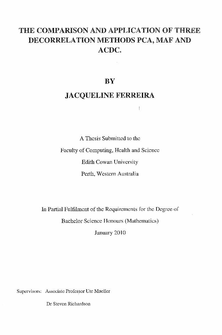
2.5 Methods Used to Assess Spatial Decorrelation.
There are a variety of ways to assess how successfully the factors have been spatially
decorrelated. For a visual assessment the cross semivariogram for each factor pair will
be graphed in order to detect any remaining spatial correlation. Perfect decorrelation is
shown when the experimental cross semivariogram factors are at zero for all lags. A
quantitative method used to measure spatial decorrelation is to calculate the absolute
deviation from diagonality ~(h), the quotient of the absolute deviation from diagonality
and the sum of the factor main diagonal entries r(h), and the spatial diagonalisation
efficiency K(h).
The deviation from diagonality at lag h, ~(h), is the sum of squares of the off-diagonal
elements of the factor experimental semivariogam matrix for all lag spacings,
K K
~(h)= LLCfp(h;k~j)) 2 ~ lhl > o. k=ljot=k
where YF denotes the experimental sem1vanogram for the factors. Perfect spatial
decorrelation occurs when ~(h) = 0 for all separation distances. A global measure is
given by the average (of ~(h) calculated at I lag spacings,
The measure of spatial decorrelation, r(h), compares the absolute sum of off-diagonal
elements of the factor experimental semivariogram matrix fp(h) with the absolute sum
of the diagonal elements calculated at each lag spacing h (Tercan, 1999). The formula
for r(h) along with the average f, of r(h) calculated at 1 lag spacings, are given by
"K "~ I" (h·k· ")I r(h) = L..k=lKL..Jo~=k YF I ~J I lhl > 0 Lk=liYF (h;k;k)l
and
J
f=yL r(hJ~ j=l
respectively. For perfect decorrelation to occur r(h)=O for all lags h.
21

Finally, the spatial decorrelation efficiency function at lag h, K(h), compares the sum of
squares of the off diagonal elements of the factor experimental semivariogram matrix
.fp(h) to the sum of squares of the off diagonal elements of the sample experimental
semivariogram matrix fz(h) (Tercan, 1999). It is given by
Perfect spatial decorrelation for all separation distances or lags h occurs when K(h)=l .
A set of matrices may be considered to be nearly in diagonal form if K(h);:::: 0.9 for all
lags h (Xie, Myers & Long, 1995). The average of K(h) for all] lag spacing is given as
The average calculated for flag spacings quantifies the overall spatial decorrelation.
22

3 Analysis This chapter discusses the exploratory and spatial analysis of the data set supplied by
Rio Tinto. The two ways in which the ten variables have been transformed will also be
discussed in this chapter. The last section of this chapter discusses the similarity and
differences between the ten variables in order to determine a suitable subset which will
be approximately decorrelated.
3.1 Data Set Background
The data set which will be used for the study has been supplied by Rio Tinto's Iron Ore
operation in Western Australia. The compositional data set contains ten variables;
aluminium oxide (Al20 3), calcium oxide (CaO), iron (Fe), the measurement of water
content of the ore (LOI), magnesium oxide (MgO), manganese (Mn), phosphorus (P),
sulphur (S), silicon dioxide or silica (Si02) and titanium dioxide or titania (Ti02). The
1885 sample measurements for each of these ten attributes come from one mining bench
in a channel iron deposit in the Pilbara region, located in the northwest of Western
Australia, approximately 1,100 km north ofPerth. The assays are from sampling ofblast
hole cuttings, where the patterns of the blast hole locations represent different phases of
mining. The original co-ordinates have been transformed, but otherwise all other
measurements are in meters. The ten variables influence the mining of iron ore as well
as the extraction of iron, and therefore need to be analysed and modelled in order to
successfully produce iron and subsequently steel.
The most important variables, in terms of saleable products, are iron, alumina and silica.
The iron content is important because it is the iron element in the ore which is
predominantly used to make steel. The main concern for mining companies would be to
identify, concentrate and mine in areas of the region which are rich in iron. Aluminium
(Al), present in Al20 3, has a number of adverse effects on the furnace operation
involved in producing iron and steel, reducing the quality of iron. Aluminium is also
very difficult to reduce once present. Therefore, it is important to identify the locations
of major Al20 3 concentrations in relation to iron, as potential clients are interested in a
high iron quality. Silica promotes the formation of gray iron which is a type of iron less
brittle and easier to finish than the more common white iron. Gray iron is preferred for
casting and is often used for housing structures while white iron is the starting material
for malleable cast iron. Thus, by mining companies knowing where areas of high silica
23
concentrations are in relation to iron deposits, they are more capable of producing a
higher quality of white and gray iron (Liddelow & Dinsdale, 1996).
The iron mineralisation occurs within the Hamersley Iron Province. The geology of this
Province is characterised by a 2,500 million year old group of late Archaean and early
Proterozoic rock formations known as the 'Hamersley Group'. The Hamersley group
was formed as a result of volcanic activity, which introduced basalt rock into the area.
Throughout its formation, ongoing transportation and weathering of the Hamersley
group led to the existence of sedimentary rocks, such as sandstone. Also during this
period, rocks with different chemical compositions were deposited in layers (Rio Tinto
Iron Ore, 2009)
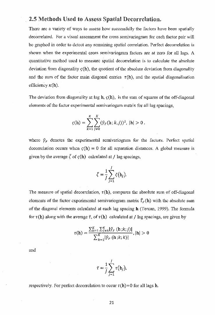
3.2 Exploratory Data Analysis
The summary statistics of the ten raw variables are given in Table 1. Each variable
comprises of 1885 observations, with no missing data. Except for Mn and Fe, the
variables are positively skewed. The severity of skewness differs for each variable, with
CaO being the most skewed and Mn being the least skewed. The kurtoses for all ten
variables are positive, indicating that the distributions are more peaked than a normal
distribution. The severity of peaks differ for each variable, with the CaO distribution
being the most peaked and S being the least peaked, compared to a normal distribution.
This is further illustrated in the histograms shown in Figure 1. The histogram for Mn
shows that the Mn distribution may be discrete.
a e -T bl 1 S ummary s ahshc or t e ten vana t .. 1" h . bl es.
Ab03 CaO Fe LOI MgO Mn p s Si02 Ti02
Mean 1.561 0.059 56.887 9.75 0.077 0.02 0.034 0.007 7.131 0.106
Median 1.21 0.06 57.18 9.73 0.07 0.02 0.033 0.007 6.97 0.07
Standard Deviation 1.202 0.026 1.96 0.411 0.027 0.006 0.007 0.003 1.752 0.102
Variance 1.446 0.001 3.84 0.169 0.001 0 0 0 3.069 0.01
Kurtosis 17.595 161.846 12.967 5.479 18.622 6.716 7.566 3.681 6.676 14.681
Skewness 3.077 8.957 -2.194 0.302 2.612 -0.229 1.521 0.981 1.11 2.932
Range 13.02 0.61 22.27 4.4 0.32 0.06 0.057 0.017 17.46 0.85
Minimum 0.33 0.03 38.21 7.34 0.03 0 0.022 0.002 3.49 0.01
Lower Quartile 0.84 0.04 56.12 9.49 0.06 0.02 0.03 0.005 5.9 0.05
Upper Quartile 1.87 0.07 58.1 9.98 0.09 0.02 0.037 0.009 8.07 0.13
Maximum 13.35 0.64 60.48 11.74 0.35 0.06 0.079 0.019 20.95 0.86
Count 1885 1885 1885 1885 1885 1885 1885 1885 1885 1885
24

llb samples: 1885 Mini mum: 0.33
Mean: Std. Dev.: 1.20
!lb samples: 1885 Minimum: 0.03 Maximum: Mean: Std. Dev.: 0.03
fib Samples: 1885 Minimum: 38.21
Mean: Std. Dev.: 1.96
Nb Sampl es: 1885 Minimum: 0 . 03
Mean : Std. Dev. : 0.03
'MgO
Figure 1-The histograms for each of the ten variables, in alphabetical order.
Shown in Figure 2 are the qq plots which are plotted against a lognormal distribution for
all variables, except Mn which is plotted against a normal distribution. The qq plots of
Al20 3, loss on ignition LOI and Si02 give the impression of following a lognormal
distribution. The qq plot for Mn shows that it may be discrete while the qq plots for S,
CaO, MgO and Ti02 indicate that these variables do not follow a lognormal
distribution. A x2 goodness of fit test with twenty two degrees of freedom, using twenty
five classes was performed. The results showed that at a five percent significance level
Si02 was the only variable which showed significant evidence that it is lognormal
(experimental x2 (30.55) <theoretical value (33.92)).
25

0
~
;;; .'l s -3
Gauss(m=0. 25 ;s=0. 59 )
g .;
0
j
Gauss (m:2 .2~;s=0.04 )
Gauss (m= -3 .39;s:O.l7 )
Gauss (m= - 2.55;9 =0 .75 )
Gauss(m=- 2 . 8S;ss0. 32)
+ ff
i
Gau ss (m=-2.6 l; s : 0.31)
-5.5 - 5.0 -4.5 -4 .0
Gauss(m:-4 .98;s=0.35)
;;; 3 3.8
0
j
3 . 6
31>.:-. 6 --:-'-:,....-:-L::---:-, '-:--. 9 ---,.:-L:-. 0 --,J-:4 . 1-----,-:J • . • 2
Gau ss(m=4 . 04;s=0 . 04 )
0.00 0.010.02 0 . 03 0.04 0.05 0.06
Gauss (m=0 .02;s =O.Ol)
Gauss {m:l. 9 4 ;.s= 0 . 24. )
Figure 2- The qq plots for each of the ten variables, in alphabetical order.
The matrix of the correlation coefficients is shown in Table 2. The highlighted red fields
indicate the variables which are highly correlated (r > 0.7). The highest correlation co
efficient is between Al20 3 and Ti02 , with a correlation of0.916. The lowest correlation
co-efficient (in terms of absolute value) is between Fe and S, with a correlation of only-
0.002. S and P are poorly correlated with all the variables, while CaO is poorly
correlated with all the variables, except MgO. Al20 3 and Fe have the highest
correlation, with being moderately or highly correlated with all the variables except for
CaO, S and P. Mn has a mixture of moderate and poor correlations with other variables.
MgO, Si02 and Ti02 have a mixture of linear correlation strengths.
26

Table 2- Correlation co-efficient matrix between the ten variables. The highlighted cells represent a I . ffi . h' h h 0 corre atwn coe tctent tgl er t an .7.
Al203 CaO Fe LOI MgO Mn p s Si02 Ti02
Al20 3 1 0.256 -0.85 0.51 0.583 -0.502 0.241 -0.106 0.541 0.916
CaO 0.256 1 -0.169 0.003 0.704 -0.121 -0.018 -0.402 0.089 0.176 Fe -0.85 -0.169 1 -0.465 -0.483 0.556 0.019 -0.002 -0.882 -0.753
LOI 0.51 0.003 -0.465 1 0.248 -0.545 0.239 -0.017 0.165 0.364 MgO 0.583 0.704 -0.483 0.248 1 -0.364 0.069 -0.424 0.316 0.424 Mn -0.502 -0.121 0.556 -0.545 -0.364 1 0.007 0.138 -0.423 -0.313 p 0.241 -0.018 0.019 0.239 0.069 0.007 1 -0.034 -0.258 0.278
s -0.106 -0.402 -0.002 -0.017 -0.424 0.138 -0.034 1 0.067 -0.024
Si02 0.541 0.089 -0.882 0.165 0.316 -0.423 -0.258 0.067 1 0.471
Ti02 0.91-6 0.176 -0.753 0.364 0.424 -0.313 0.278 -0.024 0.471 1
The base map showing the sample locations is displayed in Figure 3. The base map of
the study region shows that some areas of the region have been sampled extensively
while other areas, in particular the centre, have not been sampled as densely.
1 00
0
-1 00
-2 00 - 100 0 1 00 2 00
X (m)
Isatis
Figure 3-Base map for study region.
The spatial maps for each of the ten variables are shown in Figure 4. The colour scales
were defined via the corresponding deciles for each variable, except for Mn which was
based on the seven discrete values observed. The spatial map for Fe shows a region of
very high values on the western border. The spatial maps for Al20 3, Ti02, P and LOI do
not show any distinct areas of very high or very low values. For Si02 lower
concentrations are located on the western border. The spatial map for CaO shows that
the higher values are more concentrated on the western border, while the very low
values are more concentrated in an area in the south east. This is opposite for S. The
27

spatial map for Mn appears to have predominantly lower values. The very low values of
MgO are mainly concentrated in an area in the south east of the spatial map.
Al 203 (%)
13 35
1 0 0 2 . 77 1 00 2 . 06 1. 6 8 1. 4 1 ~ 1.21 1. 04 ><
90 - 100 7 7 -1 00
0. 63 0 . 33
X ( m) X (m)
I sat is I s a t is
Fe (%) LOI (%)
11 . 74
5 8 8 3 0 10. 2 5
58 340 1 00 1 0 . 05 1 00
9 3 0 9 . 92
5 6 5 ~
9 . 83
57 1 80 9 . 7 3
5 6 8 2 0 9 . 6 4 9 . 5 5
-1 00 9 . 43
8 2 0 9 . 2 7
-1 00
210 7 . 34
X (m) X (m)
I s a t is Isa t i s
1 00 1 00
. 3 50 0 . 06
. 1 00 0 . 05
0 . 090 ~ 0 . 04
0 . 080 0 03
>< 0 02 0 . 070 0 . 0 1
- 100 0 . 060
0 . 0 5 0 -1 00
0 . 00
0 . 030
X (m) X (m)
I s a t is I s a tis
p (%)
0 . 07 9 0 . 019
0 . 0 4 2 1 00 0 . 0 11
0 . 0 3 9 0 . 009
1 00
~ 0 . 008
0 3 3 0 . 0 07
>< 0. 006
0 . 005
- 1 00 -1 00 0 . 00 4
0. 002
X (m) X (m)
I s at is I s a tis
Si02(%) Ti02(%)
95
100 21 1 00 8 . 4 3 7 . 80
4 1 ~ 97
6 . 5 6 >< 06
6 . 1 6 05
-100 5 . 6 7 -1 00 5 . 1 3 3 . 49
X (m) X (m)
I s a ti s Isatis
Figure 4- The spatial maps for each of the ten variables in alphabetical order.
28

3.3 Spatial Analysis
The experimental semivariogram maps for each of the ten original variables were
calculated in order to identify the spatial features of each of the ten variables. An
average lag spacing of 15m using fifteen lags was used to obtain the experimental
semivariogram maps shown in Figure 5. It is clear from the experimental
semivariogram maps that the ten variables do not exhibit the same spatial behaviour.
Some ofthe variables such as LOI, Si02,Ab03 and Fe, appear to be isotropic or weakly
anisotropic, MgO and CaO appear to exhibit stronger anisotropy than LOI, Si02, Ab03
and Fe. The variables which exhibit the strongest anisotropy are Mn, P and S. There is
not a single direction of greatest continuity instead the direction of greatest continuity
varies from N20° to Nl 00° depending on the variable.
29

Al 203 CaO Fe
p s Si02
Ti02
Figure 5- The spatial maps for each of the ten variables in alphabetical order. The red shows areas of high semivariances and the blue shows areas of low semivariances.
30

3.4 Transforming the Data Set
Two types of transformations were applied to the data set. The first was a Gaussian
anamorphosis and the resultant transformation set will be denoted by subscript NS. The
other transformation involved the raw data set to be standardised by subtracting the
mean from each value in the variable and dividing the difference by the standard
deviation. For the mean and standard deviation values used for each variable, refer to
Table 1. The resultant standardised data will be denoted by. subscript St. Both
transformation methods are similar as they both transform the original variables into
variables which have a mean close to zero and standard deviation close to one. The two
transformation methods differ as standardising the raw data does not change the shape
of the original distribution, while the transformation of the raw data to normal scores
changes the original distribution of the variables into a normal distribution. In addition,
standardisation is a linear transformation, while the Gaussian anamorphosis is non
linear. The histograms of the standardised variables are shown in Figure A1 in
Appendix 1. By comparing the histograms in Figure A1 with the histograms of the raw
data in Figure 1 it is clear that the shape of the distributions of the variables have not
changed.
The transformation of the raw variables to normal scores was done in Isatis using
Gaussian anamorphosis. The Gaussian anamorphosis fit is shown in Figure 6, while
Table 3 contains the minimum, maximum and number of polynomials used for each
variable, as well as the theoretical mean and variance, and the difference between the
actual mean and theoretical mean. The parameters for each variable are shown in
Appendix 2.1.
Table 3- Minimum, maximum and number of polynomials used for each Gaussian anamorphosis fit. Number of Theoretical % error between Theoretical % error between
Min Max polynomials Mean Means Variance Variances
Al203 0 14 60 1.56 0.06406 1.445 0.06307
CaO 0 0.7 40 0.06 1.69492 0.001 32.70000
Fe 37 62 60 56.89 0.00527 3.836 0.09977
LOI 7 12 50 9.75 0.00000 0.169 0.12249
MgO 0 0.4 40 0.08 3.89610 0.001 27.80000
Mn 0 0.07 50 0.02 0.00000 0.000 0.00000
p 0 0.081 50 0.03 11.76471 0.000 0.00000
s 0 0.022 40 0.01 42.85714 0.000 0.00000
Si02 3 22 40 7.13 0.01402 3.067 0.06918
Ti02 0 0.88 50 0.11 3.77358 0.010 4.00000
31

The criteria used to determine the number of polynomials were to compare the
theoretical means and variances to the actual mean and variance, shown in Table 1 and a
visual inspection of the Gaussian anamorphosis fit for each variable. The smaller the
percentage error the better, however even though there appear to be a few high
percentage errors the slight decrease in percentage error when using a larger number of
polynomials does not warrant using the larger number of polynomials. The small
percentage difference shows how similar the actual means and variances are to the
theoretical mean and variance values, justifying the number of polynomials chosen. The
allowable range for the transformed variable was set to [ -4,4]. The histograms showing
that the variables have a normal distribution with a mean of zero and standard variation
of approximately one can be viewed in Figure A2 in Appendix 2.
;; 0.3 ~ so
; o.os
~ 0.2
~ 0.5
Figure 6-Gaussian anamorphosis for each of the ten variables in alphabetical order.
32

3.5 Subsets
The exploratory and spatial data analysis has shown how diverse the ten variables are;
· therefore using the MAF and ACDC algorithm on all ten variables may not be practical
for simulation or kriging. Instead a subset of variables needed to be selected. As the
most important variables, in terms of saleable products, are Fe, Ah03 and Si02, the
subset has to contain these three variables.
A Principal Component Analysis (PCA) and factor analysis using the correlation matrix
in SPSS was performed on the ten normal score variables. The normal scores were used
since the PCA and factor analysis are more robust when the distributions of the
variables are normal. The scree plot and correlation circle in Figure 7 show that most of
the information concerning the variability of the ten normal score variables is contained
in the first two principal components. The correlation circle of the two factors shows
that LOI, Ab03, Ti02 and Si02 are closely related. This relationship is further
highlighted by the factor pattern matrix shown in Table 4. The factor pattern matrix
contains the correlation coefficient between the variables and factors, therefore
measuring the importance of the variables to the factors, independent of the other
variables.
Scree Plot
6 7
Component Number
'" 0
Factor Plot
C•O 0
~ ' ~ oo+-----"------j----'o'-----rnr----,,.=.o,o;"""'--1 ~ 0
s 0
Factor1
0s102
Figure 7- The scree plot (left) and correlation circle (right).
The factor pattern matrix in Table 4 has fewer loadings than the original factor matrix
and therefore is easier to interpret as it only shows the highest loading for each variable.
The table shows that most of the variability for Fe, Ah03, Ti02, Si02, LOI and Mn is
present in factor one, while the variability for CaO, MgO and S can be explained in
factor two. The variability of P must be explained in one of the other factors, showing
that the statistical aspects of the variable are different to all the other variables. It would
be logical to produce two subsets, the first subset would consist of the group of
33

variables similar to that shown in factor one while the other subset would consist of the
variables shown in factor two, leaving P out.
Table 4 F - actor pattern matnx or t e two a . ~ h t: ctors ..
Factor
1 2
Fe -0.964
Alz03 0.879
Ti02 0.784
Si02 0.649
LOI 0.511 Mn -0.427 p
CaO 0.867
MgO 0.802
s -0.702
The PCA and factor analysis is a good way to determine which variables can be
grouped with each other, yet the spatial and statistical analysis has to be considered also
before a subset can be decided on. The group of variables shown in factor one appears
to make up a reasonable subset, with the exception of Mn. The reason for excluding Mn
from the subset is that it is statistically and spatial very different from the other
variables. The main concern with Mn is that it has a discrete distribution and will have
many detection limit values which may affect the normal score transformation and
hence the decorrelation. The subset of variables which was decided on was Fe, Ab03,
Si02, LOI and Ti02. These five variables were choosen because they make up the most
reasonable subset of more than four variables, which most importantly, show the most
similarity in statistical and spatial features.
34

3.6 Linearity
The MAF method does not cope well with non linear correlations or poorly correlated
variables (Rondon & Tran, 2008). Therefore, the correlation of the normal scores and
standardised variables were checked by examining the scatter plots between the five
variables in the subset, as shown in Figures 8 and 9. The corresponding correlation
coefficients are displayed in Table 5 and Table 6. The scatter plots and correlation
coefficients indicate varying degrees of linearity in the bivariate relationships between
the five variables. Linearity between the variables is better shown on the scatter plots
between the nonlial score variables than the scatter plots of the standardised variables.
The reason for this is that the normal score variables no longer have the extreme values
that the standardised variables have, as the presence of extreme values affects the
correlation coefficients and the shape of the scatter diagrams.
Table 5- The correlation coefficients for the five transformed normal scores
NS AhO~ Fe Si02 Ti02 LOI
Al203 1 -0.70229 0.3954 0.92189 0.52522
Fe -0.70229 1 -0.88765 -0.66213 -0.43529
Si02 0.3954 -0.88765 1 0.39257 0.13802
Ti02 0.92189 -0.66213 0.39257 1 0.3887
LOI 0.52522 -0.43529 0.13802 0.3887 1
Table 6- The correlation coefficients for the five standardised variables
St Al203 Fe Si02 Ti02 LOI
Al203 1 -0.84969 0.54139 0.91626 0.51003
Fe -0.84969 1 -0.88243 -0.75286 -0.46455
Si02 0.54139 -0.88243 1 0.47099 0.16513
Ti02 0.91626 -0.75286 0.47099 1 0.36436
LOI 0.51003 -0.46455 0.16513 0.36436 1
There is little difference in the correlation coefficients between the normal score
variables and standardised variables. Both of the tables show LOI to have the poorest
correlation with the other variables. This is further illustrated by the weak linear
relationship in the scatter plots which involve LOI. The scatter plots of Si02 with Ti02
and Al20 3 also show only weak correlation. The correlation coefficient between Ab03
and Fe show the two variables to have a strong negative relationship; however the
scatter plot between the two variables does not appear linear, with the upper values
showing a linear relationship but not the lower values.
35

0
~I
0
~I
0
. I
"'
-4 _,!----!-----:!-+----!:--7--7-!--~
-4 -4!----!-----:!:--+----!:--7--7-!--~
s ~I
0
~ I :i
+ +
Figure 8- The scatter plots and correlation coefficients between each of the five transformed normal score variables in the subset.
36

I ~
lsa t is
. I
0
. I
0
I
0
, . +
+
-+tr- ~I:t:+~ + -'- +
.:~ ... ++
Al203 -
+ + +
i+ +
r+
Al 203 -
+ + + : + ;+ + +
Fes
+ +"t+
+ + + .... t
t++ +
I
3
+ +
Al 203 -
. I
3
++
Fes
++ + +: -r+ .
I
~
LOI e
+ + +"* , ,. ... ,:· I 0
.,.+:: + + +
.. + +
'
Al203 -
+ ... -!#-;- ++ +
I ~
.~, 0
'.t ++ .
+· ... +
-r ,
Fe s
+ +
+ + +4-+ +
++
I
~
* ++ ++
LOI -
Figure 9- The scatter plots and correlation coefficients between each of the five standardised variables in the subset.
37

3. 7 Analysis of Experimental Semivariograms.
The experimental cross semivariogram of the normal scores and standardised subset are
shown in Fig1:1re 10. The figures show that the experimental cross semivariograms are
correlated as expected. The experimental direct semivariogram of the normal scores and
standardised subset is shown in Figure 11. A 3SLMC consisting of a nugget and two
acceptable semivariogram models '-''Ould be appropriate to capture the spatial variability
of the variables.
Experimental Cross Semivariograms of Normal Score Variables
1
0.8~-0.6
1+,--· +· ~~.~~~~~~
0.4 .!..-!-!.-..!-! I *4--.t i ·~ 0.2
-0.2
-0.4 1 'I + I I I I 4 I 1 • 1 1 -+--+
-0.6 -
-0 . 8 ·~
50 100 150 200 Lag h (m)
----+-- Fe & A1p3
----+-- Si0 2 & AI20 3
----+-- Si02
& Fe
----..-- no2
& Al2o
3
----+-- no2 & Fe
no2 & s1o2 ----+-- AII
20
3 & LOI
----+-- LOI & Fe
----+-- LOI & Si02
----+-- LOI & TI02
Experimental Cross Semivariograms of Standardised Variables
0.6 4>---+ .. • I + I :- ........... i L j t=t 0 . 4~
0.2 ; • • ------+ ~ 0~ ... 1_ 1_ ---
-0.2 -0.4_ :::~
50 100 150 200 Lag h (m)
----+-- Fe & A1p3 -+- Si02 & AI20 3
-+- Si02
&Fe
_...__ no2
& A12o
3
-+- no2 &Fe
no2 & Si02
-+- A1p3 & LOI
-+- LOI& Fe
-+- LOI & Si02
-t- LOI&TI02
Figure 10- The experimental cross semivariograms of the five normal scores (left) and standardised (right) variables.
Experimental Direct Semivariograms of Normal Score Variables Experimental Direct Semivariograms of Standardised Variables
1.15 -t- AI20 3
-- Fe
1.1 -+- Si02 -t- TI02
-+- LOI
50 100 150 200 Lag h (m)
Figure 11- The experimental direct semival"iograms of the five normal scores (left) and standardised (right) variables.
The average distance for each lag and experimental semivariogram matrices using the
normal scores and standardised variables can be viewed in Table Al and A2 in
Appendix 3. The corresponding eigenvalues for each of the experimental
semivariogram matrices are also shown in Tables A1 and A2. The eigenvalues for each
experimental semivariogram matrix are positive demonstrating that the experimental
semivariogram matrices, using the five normal scores and standardised variables
respectively, are positive definite.
38

4 Results In this chapter the results obtained throughout the study are presented. The average
spatial decorrelation results, transformation matrix and analysis of the factors for each
method will first be discussed separately. The final section will compare the spatial
decorrelation results and experimental cross semivariograms for all the methods.
4.1 Decorrelation Results
The PCA, MAF and ACDC methods were applied to the normal scores and
standardised variables for the subset, Al20 3 , Fe, Si02, Ti02 and LOI to determine
which of the methods decorrelates the subset better. The factors produced from each
method were assessed for spatial decorrelation using a number of criteria. These criteria
include a visual assessment ofthe experimental cross semivariograms ofthe factors and
plots of the absolute deviation from diagonality S'(h), the quotient of the absolute
deviation from diagonality and the sum of the factor main diagonal entries r(h) and the
spatial diagonalisation efficiency K(h) for every lag. The final criterion is a comparison
of~' the average absolute deviation from diagonality for all lags, f, an average of the
quotient of the absolute deviation from diagonality and the sum of the factor main
diagonal entries for all lags, and R, the average spatial diagonalisation efficiency for all
lags.
4.1.1 PCA Decorrelation Results
The PCA transformation using the normal scores and standardised scores was computed
using Isatis. The correlation matrix of the normal scores is
1 -0.702 0.395 0.922 0.525
-0.702 1 -0.888 -0.662 -0.435
BNs= 0.395 -0.888 1 0.393 0.138
0.922 -0.662 0.393 1 0.389
0.525 -0.435 0.138 0.389 1
The diagonal matrix of eigenvalues DrcANs and matrix of eigenvectors Q NS of BNs are
39

13.2545 0 0 0
0 I DPcA,~ ~ 1.0122 0 0 0
0 0.6400 0 0 ' 0 0 0.0657 0~0~77 0 0 0
and
0.4995 -0.2914 -0.3244 0.7085 0.2416
-0.5131 -0.3250 -0.1737 -0.1130 0.7670
QNs= 0.3927 0.6743 0.2085 -0.1020 0.5807 '
0.4789 -0.2269 -0.5185 -0.6711 0.0079
0.3220 -0.5507 0.7432 -0.1566 0.1273
respectively. The PCA transformation matrix when using the normal score variables is
the transpose of the eigenvector matrix Q and was calculated to be
0.4995 -0.5131 0.3927 0.4789 0.3220
-0.2914 -0.3250 0.6743 -0.2269 -0.5507 Q~s= -0.3244 -0.1737 0.2085 -0.5185 0.7432 .
0.7085 -0.1130 -0.1020 -0.6711 -0.1566 0.2416 0.7670 0.5807 0.0079 0.1273
The histograms of the PCA factors using the normal scores subset are shown in Figure
12. The distributions ofthe factors do not appear to follow a normal distribution. This is
supported by Kolmogorov-Smimov statistics with a Lilliefors significance level test of
normality, in Table 7, showing that there is significant evidence that the factors are not
normally distributed (sig.<0.05). The scatter plots and corresponding correlation
coefficients between the factors, shown in Appendix 4.1, confirm that the factors are
uncorrelated.
40

~ 0. 15
!
f.4 _PCA._US
Figure 12- The histograms of the PCA factors using the normal scores subset.
Table 7- The Kolmogorov-Smirnov statistics test of normality results for all the PCA factors using the normal scores subset.
Kolmogorov-Smimov
Statistic df Sig.
F1 PCA NS 0.032457 1885 0 - -
F2 PCA NS 0.022559 1885 0.026 - -
F3 PCA NS 0.084104 1885 0 - -
F4 PCA NS 0.047189 1885 0 - -
F5 PCA NS 0.037647 1885 0
The correlation matrix for the standardised scores is
1 -0.85 0.541 0.916 0.510
-0.85 1 -0.882 -0.753 -0.465
Bst= 0.541 -0.882 1 0.471 0.165
0.916 -0.753 0.471 1 0.364
0.510 -0.465 0.165 0.364 1
The diagonal matrix of eigenvalues DpcAst and matrix of eigenvectors Q st of Bs1 are
and
3.4632 0
DpcAst = 0 0 0
0 0.8857
0 0 0
0 0
0.5774 0 0
41
0 0 0
0.0659 0
0 0 0 0
0.0078

0.505 0.1385 -0.3394 -0.6989 -0.3494
-0.5197 0.1936 -0.2077 0.1586 -0.79
Q st= 0.4069 -0.5783 0.467 0.1988 -0.4923 '
0.4688 0.0715 -0.5987 0.6455 -0.0038
0.2992 0.777 0.5149 0.1736 -0.1069
respectively. The PCA transpose matrix when using the subset which had been
standardised is
0.505 -0.5197 0.4069 0.4688 0.2992
0.1385 0.1936 -0.5783 0.0715 0.777 QT-
St -0.3394 -0.2077 0.467 -0.5987 0.5149
-0.6989 0.1586 0.1988 0.6455 0.1736
-0.3494 -0.79 -0.4923 -0.0038 -0.1069
The histograms of the PCA factors using the standardised subset are shown in Figure
13. The distributions of the factors do not appear to follow a normal distribution, with
factors 1 and 3 appearing severely skewed and factors 2, 4 and 5 appearing as though
they may be slightly skewed. The scatter plots and corresponding correlation
coefficients between the factors, shown in Appendix 4.2, confirm that the factors are
uncorrelated.
~ 0. 4
~ ! 0.3 l 0.10
Figure 13- The histograms of the PCA factors using the standardised subset.
42

The measures of spatial decorrelation from the PCA transformation can be viewed in
Table 8.
Table 8-The PCA average spatial decorrelation measures using both the normal scores and standardised subset.
( f R Normal Scores Subset PCA 0.0393 0.1168 0.9938
Standardised Subset PCA 0.0182 0.076 0.9975
4.1.2 MAF Decorrelation Results
The MAF transformation was computed using Isatis. The MAF was performed using
the corresponding correlation matrix and the experimental semivariogram matrix for a
lag spacing of 15m. The correlation matrix of the normal scores used in the MAF
method is denoted as BNs and the correlation matrix for the standardised score is
denoted as Bst· The choice of 15m was made because this lag spacing best reflected the
data spacing. The experimental variance/covariance matrix of the normal scores for a
lag spacing of 15m (h=15m) used in the MAF is
1.81595 -1.29358 0.72332 1.63417 1.03795
-1.29358 1.61754 -1.36892 -1.19928 -0.73897
C(h)Ns= 0.72332 -1.36892 1.53154 0.69563 0.144 ' 1.63417 -1.19928 0.69563 1.63087 0.90966
1.03795 -0.73897 0.144 0.90966 1.63043
and the experimental variance/covariance matrix for the standardised scores is
1.78711 -1.55377 1.00519 1.62297 0.99212
-1.55377 1.69742 -1.43589 -1.37398 -0.78994
C(h)st= 1.00519 -1.43589 1.58067 0.8607 0.19738
1.62297 -1.37398 0.8607 1.64359 0.8461
0.99212 -0.78994 0.19738 0.8461 1.64241
The MAF transformation matrix for the normal scores subset is
-1.3636 1.8751 0.0589 1.9508 -0.9432
-0.4533 0.8892 -4.0597 0.9263 -1.8273 xT-Ns- -0.6262 -0.2707 -2.9026 0.9741 -1.7503 '
1.8943 -1.0675 -1.2877 -0.7616 0.6582
-0.6058 -0.3019 -1.1859 -0.2511 0.475
43

while the MAF transformation matrix using the standardised subset is
-1.564 3.369 -2.0569 -2.0027 -1.1812
-0.1431 3.2215 -7.8644 -2.1563 -2.0236 xT-s- -0.2403 1.002 -5.0363 -1.8031 -1.7193 .
2.0505 -1.06 -1.0208 0.3565 0.7166
-0.429 -0.1816 -1.6203 -0.0204 0.5043
The histograrns of the MAF factors using the normal scores subset and standardised
subset are displayed in Figure 14 and Figure 15, respectively. MAF factor 2 using the
normal scores subset appears to be the only MAF factor which may follow a normal
distribution. This is confirmed by the Kolmogorov-Smimov statistics with a Lilliefors
significance level test of normality (see Table 9) showing that at a 5% significance level
there is enough evidence to suggest that factor 2 may be normally distributed
(sig.>0.05). The distributions of the MAF factors using the standardised subset appear
to be skewed, with factor 4 showing to be severely skewed.
n_MAF_us
: •.lS
! ::: i ~ 0 10
FS_KAF_US
Figure 14- The histograms of the MAF factors using the normal scores subset.
44

MAF Factors using the Standardised Subset ,-------,
!lbsar:;plf!l:lSaS
H~~~~:;~ 1 -~~~~:o !-------,------,------,
scd..Dev., 1.000
r 0.2
Figure 15- The histograms of the MAF factors using the standardised subset.
Table 9- The Kolmogorov-Smirnov statistics test of normality results for all the MAF factors using the normal scores subset
Kolmogorov-Smimov
Statistic Df Sig.
F1 MAF NS 0.06471 1885 0 - -
F2 MAF NS 0.020641 1885 0.059 - -
F3 MAF NS 0.0309 1885 0 - -
F4 MAF NS 0.039033 1885 0 - -
F5 MAF NS 0.039735 1885 0
The scatter plots and corresponding correlation coefficients between the MAF factors
using the normal scores and standardised variables are shown in Appendix 4.3 and 4.4,
respectively. The scatter plots and corresponding correlation coefficients confirm that
the factors are uncorrelated.
The results of the average spatial decorrelation measures for the MAF factors using the
normal score subset and standardised subset are shown in Table 10. The spatial
decorrelation from the MAF transformation performed better than that from PCA (Table
8) for all the measures, except for r using the standardised subset.
Table 10- The MAF average spatial decorrelation measures using both the normal score subset and standardised subset.
( f R Normal Sco:t;es Subset MAF 0.0164 0.0907 0.9976
Standardised Subset MAF 0.0177 0.0797 0.9978
45

4.1.3 ACDC Decorrelation Results
The ACDC method was performed in Matlab. The target matrices to be diagonalised
consisted of fifteen symmetric positive definite matrices, calculated from the
experimental semivariograms of the five normal scores or standardised variables
respectively using a lag spacing of 15m. The ACDC function in Matlab was executed
initially using the call [A,D,Nit,Cls]=acdc(M,w,TOL), where A is the diagonalising
matrix, D is the K X ] matrix of diagonal values, Nit is the number of full iterations,
Cis is the vector of Nit Cis values, M is the array of target matrices (K X K X ]), w
(1 x]) is the weight vector, TOL is the tolerance which was set to lxl0-16• The initial
diagonalising matrix was not specified in the call; therefore it was automatically set to
the identity matrix. The ACDC function call in Matlab specifying the initial guess for
the diagonalising matrix Ao, was [A,D,Nit,Cls]=acdc(M,w,TOL,AO). The original
ACDC algorithm written by Yeredor (2004) was changed slightly, as the maximum
number of allowed full iterations was increased from 50 to 100,000. The MATLAB
code used can be viewed in Appendix 6.
The weight vector plays a significant part in the ACDC algorithm as it contains the
weights assigned to the corresponding target matrices. The weight vector was used to
systematically reduce the number of semivariogram matrices used in the
diagonalisation. The first weight vector ensured that all fifteen target matrices were
included; the next weight vector was reduced to that the first fourteen matrices were
approximately simultaneously diagonalised by making the weight of the last target
matrix zero. For every subsequent ACDC performed the last non zero weight was set to
zero until only the first target matrix remained. This process was carried out both for the
normal scores subset and standardised subset. The weight vectors and resulting values
of ~, f and R using the normal score subset and standardised subset are summarised in
Table 11 and Table 13, respectively.
With respect to ~and f , the best decorrelation for ACDC using the normal scores was
obtained using the first eleven semivariogram matrices, while for R the use of the first
thirteen semivariogram matrices yielded the best result. These values are highlighted on
Table 11 by having a border around them. The percentage difference between the values
for~~ f and R using thirteen or eleven semivariogram matrices was 117.03%, 90.86%,
0.11 %, respectively. Therefore using the first eleven semivariogram matrices yielded
the best results for ACDC using the normal scores. A visual inspection of the cross
46

semivariogram factors and spatial decorrelation plots (see Appendix 5) confirmed the
conclusion. The f value using the first eleven semivariogram matrices is lower than the
corresponding MAF f value ( :::0.0907). The R. using the first thirteen semivariograms is
higher than the corresponding MAF R. value ( ;::£).9976).
Table 11- The ACDC weights and corresponding average spatial decorrelation values using the normal scores b Th b d . d' h b . I d I . l £ h l su set. e or ers m 1cate t e est spatia ecorre atwn va ues or t at co umn.
Number ofExp. Weight vector Average Spatial Decorrelation Values semivariogram matrices used ( f K
15 [1 1 1 1 1 1 1 1 1 1 1 1 1 1 1] 0.0656 0.136 0.9893 14 [1 1 1 1 1 1 1 1 1 1 1 1 1 1 0] 0.076 0.1548 0.9874 13 [1 1 1 1 1 1 1 1 1 1 1 1 1 0 0] 0.0726 0.1567 I 0.9981 12 [1 1 1 1 1 1 1 1 1 1 1 1 0 0 0] 0.1361 0.1559 0.9783 11 [1 1 1 1 1 1 1 1 1 1 1 0 0 0 0] 0.019 I 0.0588 I 0.997 10 [1 1 1 1 1 1 1 1 1 1 0 0 0 0 0] 0.0507 0.1099 0.9924 9 [1 1 1 1 1 1 1 1 1 0 0 0 0 0 0] 0.0578 0.112 0.9915 8 [1 1 1 1 1 1 1 1 0 0 0 0 0 0 0] 0.0592 0.1073 0.9913 7 [1 1 1 1 1 1 1 0 0 0 0 0 0 0 0] 0.0434 0.1377 0.9937 6 [1 1 1 1 1 1 0 0 0 0 0 0 0 0 0] 0.0461 0.1125 0.9933 5 [1 1 1 1 1 0 0 0 0 0 0 0 0 0 0] 0.1188 0.16 0.9829 4 [1 1 1 1 0 0 0 0 0 0 0 0 0 0 0] 0.0677 0.1476 0.9903 3 [1 1 1 0 0 0 0 0 0 0 0 0 0 0 0] 0.0938 0.1727 0.9865 2 [1 1 0 0 0 0 0 0 0 0 0 0 0 0 0] 0.3753 0.398 0.9458 1 [1 0 0 0 0 0 0 0 0 0 0 0 0 0 0] 0.2839 0.251 0.959
For ACDC the transformation matrix is the inverse of the diagonalising matrix A. The
ACDC transformation matrix using the normal scores subset and including the first
eleven matrices is given as
1.584 -0.4104 -0.0845 -1.025 -0.5786 0.606 2.2174 1.3374 0.4762 0.3463
A-I= NS
-1.4133 -3.0201 -2.6701 0.8501 0.7002
-2.5549 -1.8318 -1.5408 2.6954 -0.9458
-1.7193 1.9411 2.9292 1.6409 1.2326
The histograms of the corresponding factors are displayed in Figure 16. The
distributions of the factors do not appear to be normal. This is supported by
Kolmogorov-Smimov statistics with a Lilliefors significance level test of normality, in
Table 12, showing that there is significant evidence that the factors are not normally
distributed (sig.<0.05). The scatter plots and corresponding correlation coefficients
between the factors, shown in Appendix 4.5, confirm that the factors are uncorrelated.
47

Fl_ ACOC_JIS
l 0"
;;, 0.10
Figure 16- The histograms of the ACDC factors using the normal scores subset and first eleven experimental semivariogram matrices.
Table 12- The Kolmogorov-Smirnov statistics test of normality results for all the ACDC factors using the normal scores subset and fi I · I · · · 1rst e even expenmenta sem1vanogram matnces.
Kolmogorov-Smimov
Statistic Df Sig_.
F1 ACDC NS 0.025149 1885 0.008 -
F2 ACDC NS 0.044756 1885 0 - -
F3 ACDC NS 0.044239 1885 0 - -
F4 ACDC NS 0.054831 1885 0 -
F5 ACDC NS 0.022927 1885 0.022
With respect to (and R, the best decorrelation for ACDC using the five standardised
variables was obtained using the first seven semivariogram matrices, while for i the
use of the first nine semivariograms yielded the best result. The percentage difference
between the values for (, i and K using seven or nine semivariogram matrices was
15.51%, 17.6% and 0.08%, respectively. A visual inspection of the experimental cross
semivariogram factors and spatial decorrelation plots (see Appendix 5) between using
seven or nine semivariogram matrices showed the decorrelation using seven
semivariogram matrices to be better than that using nine semivariogram matrices.
Therefore using the first seven semivariogram matrices yielded the best results for
ACDC using the five standardised variables. None of three average spatial decorrelation
values in Table 13 were better than the corresponding MAF average spatial
48

decorrelation values, therefore the MAF method is the better method when using just
the standardised variables.
Table 13- The ACDC weights and corresponding average assessment values using the standardised subset. The b d . d" t h b . 1 d 1 . 1 ~ h 1 or ers m 1ca e t e est spatia ecorre atwn va ues or t at co umn.
Number ofExp. Weight vector Average Spatial Decorrelation Values sem1vanogram matrices used ( f R
15 [1 1 1 1 1 1 1 1 1 1 1 1 1 1 1] 758480 1.8403 -100410 14 [1 1 1 1 1 1 1 1 1 1 1 1 1 1 0] 11948000 0.8145 -1582100 13 [1 1 1 1 1 1 1 1 1 1 1 1 1 0 0] 105820000 0.7761 -14008000 12 [1 1 1 1 1 1 1 1 1 1 1 1 0 0 0] 21018000 0.7986 -2781900 11 [1 1 1 1 1 1 1 1 1 1 1 0 0 0 0] 0.4708 0.3566 0.9364 10 [1 1 1 1 1 1 1 1 1 1 0 0 0 0 0] 0.2866 0.2218 0.9618 9 [1 1 1 1 1 1 1 1 1 0 0 0 0 0 0] 0.0382 I 0.0793 I 0.9951 8 [1 1 1 1 1 1 1 1 0 0 0 0 0 0 0] 0.0394 0.0997 0.9952 7 [1 1 1 1 1 1 1 0 0 0 0 0 0 0 0] 0.0327 I o.o946 I 0.9959 6 [1 1 1 1 1 1 0 0 0 0 0 0 0 0 0] 0.0379 0.1118 0.9954 5 [1 1 1 1 1 0 0 0 0 0 0 0 0 0 0] 0.0686 0.1083 0.992 4 [1 1 1 1 0 0 0 0 0 0 0 0 0 0 0] 0.1138 0.1738 0.9867 3 [1 1 1 0 0 0 0 0 0 0 0 0 0 0 0] 0.193 0.2137 0.977 2 [1 1 0 0 0 0 0 0 0 0 0 0 0 0 0] 0.2199 0.2534 0.974 1 [1 0 0 0 0 b 0 0 0 0 0 0 0 0 0] 0.3312 0.2716 0.9596
The ACDC transformation matrix
2.5068 4.3366 3.068 -0.2417 0.5622
-1.2471 -7.5238 -4.2105 -1.7231 -1.9398 A-1=
St 2.7725 1.6742 0.1346 -1.2494 -0.326
-1.2477 -0.0761 -0.3075 2.0621 -0.6093
-1.9128 -4.9115 -3.386 0.3537 0.0682
is the transformation matrix calculated when the ACDC method including the first
seven experimental semivariogram matrices is used on the standardised subset. The
histograms of the ACDC factors are displayed in Figure 17 and show all the
distributions of the factors to be skewed. The scatter plots and corresponding correlation
coefficients between the factors, shown in Appendix 4.6, confirm that the factors are
uncorrelated.
49

~ 0.15
!
Figure 17- The histograms of the ACDC factors using the standardised subset.
The effect of using an initial guess for the diagonalising matrix Ao with the ACDC
algorithm was also explored in conjunction with changing the weights as done
previously. The initial guess decided on was the eigenvector matrix obtained from the
PCA using the normal scores and standardised subset. The PCA eigenvalue matrix was
chosen because the transpose of the PCA already transforms the variables into
approximately uncorrelated factors , therefore the ACDC method would improve on the
PCA eigenvalue matrix. The PCA eigenvector matrix when using the normal score
subset was calculated to be
0.4995 -0.2914 -0.3244 0.7085 0.2416
-0.5131 -0.3250 -0.1737 -0.1130 0.7670
AoNs=QNs= 0.3927 0.6743 0.2085 -0.1020 0.5807
0.4789 -0.2269 -0.5185 -0.6711 0.0079
0.3220 -0.5507 0.7432 -0.1566 0.1273
The PCA eigenvector matrix using the standardised subset is
0.505 0.1385 -0.3394 -0.6989 -0.3494
-0.5197 0.1936 -0.2077 0.1586 -0.79
Aost=Qst= 0.4069 -0.5783 0.467 0.1988 -0.4923 .
0.4688 0.071 5 -0.5987 0.6455 -0.0038
0.2992 0.777 0.5149 0.1736 -0.1069
The results of the average spatial decorrelation measures using the ACDC method on
either the normal scores subset or standardised subset while changing the weights, as
50

well as including the initial diagonalising matrix A0NS or A08t for the corresponding
subset are shown in Table 14 and 16, respectively.
All three average spatial decorrelation results (Table 14) using the first ten, nine, six and
five experimental semivariogram matrices are better than the corresponding average
spatial decorelation results obtained for the MAF, shown in Table 10. In addition, the
values (and K. using thirteen, twelve, eleven and eight semivariogram matrices are
better than the corresponding MAF ( (::0.0164) and K. values (;:£).9976), but not for the
values off, which was lowest using the first seven experimental semivariogram
matrices. Overall, because there are so many options of good spatial decorrelations, the
experimental cross semivariograms of the factors and spatial decorrelation plots were
also examined to determine which number of included experimental semivariogram
matrices gives the overall best ACDC spatial decorrelation using the normal scores and
A0NS. The experimental cross semivariograms for every factor calculated with the
corresponding spatial decorrelation plots are shown in Appendix 5. The experimental
cross semivariogram factors and spatial decorrelation plots using the first ten, nine, six
and five matrices were compared and the best decorrelated cross semivariogram factors
resulted using the first nine semivariogram matrices. The reason for choosing the first
nine experimental semivariogram matrices was because the experimental cross
semivariograms of the factors appear to be more decorrelated for the first eight lags. For
most of the ACDC experimental cross semivariogram factors using the matrixA0 NS'
there is a linlc between the number of experimental semivariogram matrices used for
decorrelation and the number of lags showing excellent spatial decorrelation.
51

Table 14- The ACDC weights and corresponding average assessment values using the normal scores subset and the matrix A0 The borders indicate the best spatial decorrelation values for that column M~'
Number ofExp. Weight vector Average Spatial Decorrelation Values semtvanogram matrices used ( f R
15 [1 1 1 1 1 1 1 1 1 1 1 1 1 1 1] 207230 1.9721 -31720 14 [1 1 1 1 1 1 1 1 1 1 1 1 1 1 0] 0.0173 0.1633 0.9972 13 [1 1 1 1 1 1 1 1 1 1 1 1 1 0 0] 0.0139 0.1455 0.9978 12 [1 1 1 1 1 1 1 1 1 1 1 1 0 0 0] 0.013 0.1021 0.998 11 [1 1 1 1 1 1 1 1 1 1 1 0 0 0 0] 0.0117 0.0909 0.9982 10 [1 1 1 1 1 1 1 1 1 1 0 0 0 0 0] 0.0132 0.0894 0.9981 9 [1 1 1 1 1 1 1 1 1 0 0 0 0 0 0] 0.0147 0.0883 0.9979 8 [1 1 1 1 1 1 1 1 0 0 0 0 0 0 0] 0.0087 I 0.0934 I 0.9987 7 [1 1 1 1 1 1 1 0 0 0 0 0 0 0 0] 0.0172 0.0876 0.9975 6 [1 1 1 1 1 1 0 0 0 0 0 0 0 0 0] 0.0151 0.0813 0.9978 5 [1 1 1 1 1 0 0 0 0 0 0 0 0 0 0] 0.0144 I 0.0782 I 0.9979 4 [1 1 1 1 0 0 0 0 0 0 0 0 0 0 0] 0.0226 0.0933 0.9968 3 [1 1 1 0 0 0 0 0 0 0 0 0 0 0 0] 0.0338 0.1102 0.9951 2 [1 1 0 0 0 0 0 0 0 0 0 0 0 0 0] 0.0775 0.1974 0.9888 1 [1 0 0 0 0 0 0 0 0 0 0 0 0 0 0] 0.0282 0.1008 0.9959
The ACDC transformation matrix using the normal scores, A0 N8matrix and including
the first nine experimental semivariogram matrices is
2.364 1.3825 1.5983 -1.3335 -0.4226
1.9548 3.012 1.2632 -0.3682 0.4095 -1
A NS = -1.3222 0.418 0.1076 2.1648 -0.4263 AoNs -0.2409 0.6133 0.5944 0.3454 0.3787
-0.003 -1.4094 -1.176 -0.0893 -0.1312
The histograms of the factors using the normal scores subset and matrix AoNs are shown
in Figure 18. The distributions of the factors do not appear to be normal. This is
supported by Kolmogorov-Smimov statistics with a Lilliefors significance level test of
normality, in Table 15, showing that there is significant evidence that the factors are not
normally distributed (sig.<0.05). The scatter plots and corresponding correlation
coefficients between the factors, shown in Appendix 4. 7, confirm that the factors are
uncorrelated.
52

He an: Std.Oe'l.: 1.053
Figure 18- The histograms of the ACDC factors using the normal scores subset, the matrix AoNs and first nine experimental semivariogram matrices.
Table 15- The Kolmogorov-Smirnov statistics test of normality results for all the ACDC factors using the normal scores subset the matrix A and first nine experimental semivariogram matrices.
' ONs
Kolmogorov-Smimov
Statistic Df Sig.
F1_ACDC_NS+A0 0.024361 1885 0.011 F2_ACDC_NS+A0 0.05146 1885 0 F3_ACDC_NS+A0 0.063552 1885 0 F4_ACDC_NS+A0 0.039039 1885 0
F5 ACDC NS+A0 0.052242 1885 0
The best spatial decorrelation measures for ACDC using the standardised variables and
Aost are obtained using the first four experimental semivariogram matrices (Table 16).
The average spatial decorrelation resulting from using the first four experimental
semivariogram matrices is also overall the best spatial decorrelation result achieved.
The values of (and K. using eight, six and one experimental semivariogram matrix are
better than the value of ( ( :::0.0177) for MAF and the value of K. for MAF ( ~.9978).
The value off using five semivariogram matrices was better than the corresponding
PCA value off ( :::0.0760).
When the matrix A0 5t and the first experimental semivariogram matrix in the ACDC
algorithn1 were used the average spatial decorrelation results were very similar to the
results calculated from the MAF method used on the standardised variables.
53

Table 16- The ACDC weights and corresponding average assessment values using the standardised subset, the matrix A081 and first four experimental semivariogram matrices. The borders indicate the best spatial
decorrelation values for that column.
Number ofExp. Weight vector Average Spatial Decorrelation Values semivariogram matrices used ( f R
15 [1 1 1 1 1 1 1 1 1 1 1 1 1 1 1] 374650 1.8683 -49593 14 [1 1 1 1 1 1 1 1 1 1 1 1 1 1 0] 741010 1.6695 -98073 13 [1 1 1 1 1 1 1 1 1 1 1 1 1 0 0] 1250500 1.4464 -165470 12 [1 1 1 1 1 1 1 1 1 1 1 1 0 0 0] 1321300 1.0632 -174780 11 [1 1 1 1 1 1 1 1 1 1 1 0 0 0 0] 152240 1.1424 -20134 10 [1 1 1 1 1 1 1 1 1 1 0 0 0 0 0] 0.0432 0.2018 0.9943 9 [1 1 1 1 1 1 1 1 1 0 0 0 0 0 0] 0.0256 0.0916 0.9964 8 [1 1 1 1 1 1 1 1 0 0 0 0 0 0 0] 0.0103 0.0823 0.9986 7 [1 1 1 1 1 1 1 0 0 0 0 0 0 0 0] 0.0186 0.0922 0.9975 6 [1 1 1 1 1 1 0 0 0 0 0 0 0 0 0] 0.0153 0.0956 0.9981 5 [1 1 1 1 1 0 0 0 0 0 0 0 0 0 0] 0.0203 0.0729 0.9976 4 [1 1 1 1 0 0 0 0 0 0 0 0 0 0 0] 0.0076 I 0.0612 I 0.9991 3 [1 1 1 0 0 0 0 0 0 0 0 0 0 0 0] 0.0201 0.082 0.9976 2 [1 1 0 0 0 0 0 0 0 0 0 0 0 0 0] 0.0219 0.1077 0.9974 1 [1 0 0 0 0 0 0 0 0 0 0 0 0 0 0] 0.0177 0.0792 0.9978
The factors of the ACDC method using the standardised subset, Aost matrix and
including the first four experimental semivariogram matrices were calculated using the
transformation matrix
3.2673 4.9355 3.8439 -0.1762 0.9583
-0.5603 -1.8103 -1.8559 0.144 0.3372 -1
A St = 2.3918 3.5799 1.6771 -0.2971 0.0895 Aost -0.8222 -0.481 -0.3298 0.8346 -0.1925
0.0178 -1.654 -1.1417 -0.5042 -0.4807
The histograms of the ACDC factors are shown in Figure 19. The distributions of
factors show all the factors to be skewed with factors 1, 3 and 4 being severely skewed.
The scatter plots and corresponding correlation coefficients between the factors, shown
in Appendix 4.8, confirm that the factors are uncorrelated.
54

n_Acoc_s Fl_Acoc_s
!"!t!!3n, o.ooo Std.Oev.: 0.650
Figure 19- The histograms of the ACDC factors using the standardised subset and the matrix Aost·
4.2 Comparison of Results
Graphs of all the values (, f and K. calculated from the factor semivariogram matrices
that were produced by the three methods using the normal scores subset and
standardised subset are shown in Figure 20. Here the values (, f and K. are treated as
functions of the number of zeros in the weight vector. The three graphs on the left
correspond to the normal scores, those to the right corresponds to standardised
variables. The graphs in Figure 20 further illustrate the best spatial decorrelation
discussed in the previous section for each different ACDC method performed.
0 _ 1[Averag~e ~Results using Normal Scores ~ACDC 0.08 ~ ACDC+AONS
g( 0.06 --MAF
"' - -PCA ~ :~~~ c__ _ __ ___J
~~G~r=rcz:Jc_-_-_-_-_~:_'~-~-+A-OS_jl 0 2 4 6 8 10 12 14 0 2 4 6 8 10 12 14
Number of Zeros Number of Zeros
~ ~:o c_-_-_-_~ '-~~-~-~+-AO-NS-' f ~:c· 'O :_-_-_-_~:_'~-~-+A-OS_jl 0 2 4 6 8 10 12 14 0 2 4 6 8 10 12 14
Number of Zeros Number of Zeros
Average" Results using Normal Scores Average "Results using Standardised data
1 ~ACDC+A051 • r\1 .-~--AC_D_C_--,
t ::J~~ ~ ~ ---~~= 0 2 4 6 8 10 12 14
Number of Zeros Number of Zeros
Figure 20- The plots of all the average spatial decorrelation results. The x axes title 'Number of Zeros' represent the number of zeros present in the weight vector, as shown in Tables 11, 13, 14 and 16.
55

In general, the decorrelation results for ACDC are better when the data are transformed
to normal scores prior to the the application of the algorithm. For both approaches,
ACDC with the use of the diagonalising matrix of the correlation matrix as the initial
guess outperforms ACDC with the identity matrix as the intial diagonaliser. For the
normal scores variables the ACDC method performs at least as well as MAF, as long as
more than the first four experimental semivariogram matrices are used. For the
standardised variables, the ACDC method shows worse decorrelation than MAF when
the ACDC algorithm is initialised with the identity matrix. The performance is
comparable to MAF, when the initialising matrix is the diagonalising matrix of the
correlation matrix and no more than eleven experimental semivariogram matrices are
used for calculating the transformation matrix. At eleven lags, most of the
semivariograms and cross-variograms ofmost ofthe variables have reached the sill. The
experimental cross semivariograms ?f the PCA and MAF factors as well as the factors
of the ACDC methods which produced the best decorrelation measures are shown in
Figure 21.
Perfect spatial decorrelation occurs when the experimental cross semivariogram factors
are equal to zero for all lags. For PCA the spatial decorrelation is good for the majority
of the factors except for two or three factor pairs which still exhibit correlation. For
MAF, the spatial decorrelation is perfect at the second lag with the other lags showing
slight correlation between the factor pairs. The ACDC factors which included an initial
diagonalising matrix showed the best spatial decorrelation for both the normal scores
and standardised scores. The best overall spatial decorrelation was obtained by the
ACDC factors including the Aost using the standardised subset, while the worst spatial
decorrelation was shown by the experimental cross semivariogram factors for the
ACDC factors pairs using the standardised subset.
The plots of the corresponding measures of spatial decorrelation (((h), r(h) and K(h))
are displayed in Figure 22. The plots of K(h) appear to be very similar for all the plots.
The MAF spatial decorrelation plot for ((h) and r(h) is perfect at the second lag with
a slight increase occurring after the eleventh lag. For all the MAF and ACDC
((h) and r(h) plots, the values of ((h) and r(h) increase after the eleventh lag and
eighth lag for the ACDC using the normal scores and the matrix A0 NS' with varying
severity of increase. The best decorrelation plot is the ACDC transformation on the
standardised subset which included the matrix Aost·
56

Cross Semivariograms of PCA Factors using Normal Scores 0.15 ,--------,
0. 1
0.05
50 100 Lag h (m)
150 200
-+- PC1-PC2 -+- PC1 -PC3 -+- PC2-PC3 - +-- PC1-PC4
-+- PC2-PC4 PC3-PC4
-+- PC1-PC5 -+- PC2-PC5 -+- PC3-PC5 -+- PC4-PC5
Cross Semivariograms of MAF Factors using Normal Scores 0.15 ,-- - - -,
0.1
;;:
-0.1
50 100 Lag h (m)
-+- M1-M2 -+- M1-M3 --+- M2-M3 --+- M1-M4 -+- M2-M4
M3-M4 -+- M1-M5
--+- M2-M5 ~- M3-M5
--+- M4-M5
150 200
Cross Semivariograms of ACDC Factors using Normal Scores 0.15
0.1 \
0~~-· ~ . ~ 0 . ;;: . . : . . ',
. \ . . 4~ .
\ .
-0.1
50 100 150 200 Lag h (m)
--+- AC1-AC2 -+- AC1-AC3
--+- AC2-AC3 --+- AC1-AC4 -+- AC2-AC4
AC3-AC4 -+- AC1-AC5 --+- AC2-AC5 -+- AC3-AC5 --+- AC4-AC5
Cros~ 1~emivariograms of ACDC Factors using Normal Scores and AONs
-+- AC1-AC2
0.1
0.05
50 100 Lag h (m)
-+- AC1-AC3 -+- AC2-AC3 -~- AC1-AC4
-+- AC2-AC4 AC3-AC4
--t- AC1-AC5 -+- AC2-AC5 -+- AC3-AC5 --+- AC4-AC5
150
Cross Semivariograms of PCA Factors using Standardised Scores 0.15
-+- PC1-PC2 -+- PC1-PC3 -+- PC2-PC3 -+- PC1-PC4 -+- PC2-PC4
• PC3-PC4
-+- PC1 -PC5 -+- PC2-PC5 -+- PC3-PC5 -+- PC4-PC5
-0.05
-0.1
50 100 150 200 Lag h (m)
Cross Semivariograms of MAF Factors using Standardised Scores 0.15
-+- M1-M2 -+- M1-M3
0.1 --+- M2-M3 -+-- M1-M4
-4 -+- M2-M4 M3-M4
-+- M1-M5 --+- M2-M5 -+- M3-M5
f_ --+- M4-M5
-0.1
50 100 150 200 Lag h (m)
Cross Semivariograms of ACDC Factors using Standardised Scores 0.15
50 100 Lag h (m)
150
--+- AC1 -AC2 --+- AC1-AC3 --+- AC2-AC3 -+- AC1-AC4 --+- AC2-AC4
AC3-AC4 --t- AC1-AC5 --+- AC2-AC5 --4- AC3-AC5 -+- AC4-AC5
Cross ;1~mivariograms of ACDC Factors using Standardised Scores and A051
--+- AC1-AC2
0.1
-0.1
50 100 Lag h (m)
150 200
--+- AC1-AC3 --+- AC2-AC3 -+- AC1-AC4 -+- AC2-AC4
·· AC3-AC4 -+- AC1-AC5 --+- AC2-AC5 -+-- AC3-AC5 --+- AC4-AC5
Figure 21- The experimental cross semivariograms of the factors obtained for each of the methods
57
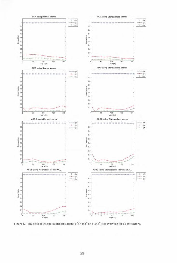
PC.A using Normal scores
1 0 0 0 0
0.9
0.8
0.7
0.6
0.5
0.4
0.3
0.2
PC.A using Standardised scores
0.9
0.8
0.7
0.6
0.5
0.4
0.3
0.2
0.1 0.1 .._.,._-+--+---+---.>---<1--+-......__~
~~~ 50 100 150 200 50 100 150
M.AF using Normal scores M.AF using Standardised scores
1 0 0 0 0 . ~ . ~
Q8 Q8
Q7 Q7
Q5 Q5
Q3 Q3
Q2 Q2
0.1 · -4\. y ............. ~--+...--.,-+--+---...~__......~ - "'-/-. ....--... v -='
50 100 150 200 50 100 150 Lag h (m) Lag h (m)
.ACDC using Normal scores .ACDC using Standardised scores
1 0 D D 0
0.9 0.9
0.8 0.8
0.7 0.7
0.6 0.6
0.5 0.5
0.4 0.4
0.3 0.3
0.2
0.1 0.1
50 100 150 200 50 100 150 Lag h (m) Lag h (m)
2oo
200
200
.ACDC using Normal scores and .AONs .ACDC using Standardised scores and .A051
1 0 0 0 0
0.9
0.8
0.7
0.6
0.5
0.4
0.3
0.2
0.1 ~---+---.....-......-0~~~~~-~~~~~F=~~~----~
0 50 100 150 200 Lag h (m)
0.8
0.7
0.6
0.5
0.4
0.3
0.2
50 100 150 200 Lag h (m)
Figure 22- The plots of the spatial decorrelation ({(h), r(h) and K(h)) for every lag for all the factors.
58

5 .. Discussion and Conclusion In this chapter the various transformation methods and effectiveness for spatial
decorrelation will be reviewed, and a conclusion will be made on which of the methods
seemed to be the most effective for the data set.
Linear transformation methods can be used to transform spatially correlated variables
into spatially decorrelated factors which can then be modelled and simulated using
univariate geostatistical techniques, which have less complexity than multivariate
techniques. Linear transformation methods, such as PCA and MAF, are established
techniques used for spatial decorrelation in geostatistics; however these methods have
limitations, such as not performing well with poorly correlated data, which has led to
the exploration of other linear transformation methods. In this thesis we looked at
whether a more general and recent approach for spatial decorrelation using the ACDC
method is able to decorrelate a multivariate data set of more than four variables better
than the currently used MAF method. The ACDC method is appealing as it has no
distributional requirements and there is no joint modelling required. In addition, we also
explored whether it is beneficial to transform the variables into normal scores rather
than standardised scores before decorrelating the variables.
PCA is very convenient and easy to implement, yet it is very limited as spatial
decorrelation is only guaranteed when the spatial dependence of the variables under
consideration can be modelled by an intrinsic model of co-regionalisation. Although,
the method still provided reasonable spatial decorrelation, it may be more suited to
performing multivariate data analysis prior to decorrelation via other methods (e.g.
MAF or ACDC).For example, PCA was used to select the variable subset to be
decorrelated, and to provide an initial guess for a diagonalising matrix in the ACDC
method. The spatial decorrelation was acceptable, considering that the data are not
intrinsically correlated, with only a few factor pairs showing correlation. The factors
obtained from applying the PCA method on the standardised variable appeared to have
better spatial decorrelation than those obtained from the PCA method using the
transformed normal scores.
The MAF method has been shown to overcome the limitations of the PCA provided that
the covariance function of the variables is fully characterised by a 2SLMC. In this thesis
the MAF method involved an experimental variance/covariance matrix and the
correlation matrix in which the factors were derived via two successive PCAs. The
59

spatial decorrelation obtained using MAF achieved better decorrelation results than
PCA and the ACDC using the standardised variables. The MAF using the standardised
variables achieved slightly better decorrelation results than the MAF using the normal
scores.
The MAF method does not cope well with poor correlation and non linear correlations
between variables. Poor correlation was exhibited between LOI and the other four
variables; this may have affected the efficiency of the MAF method. However, the
spatial decorrelation was good overall, so the impact of LOI on the results cannot have
been that strong.
The ACDC method is a more general approach to the spatial decorrelation of a set of
variables, and is not constrained to determining an orthogonal transformation matrix.
The ACDC method was used to simultaneously approximately diagonalise a set of up to
fifteen experimental semivariogram matrices calculated for lag spacings in multiples of
15m. The ACDC method showed the best and worst spatial decorrelation in comparison
to PCA and MAF. The spatial decorrelation for the ACDC factors using the
standardised variables showed the worst spatial decorrelation, regardless of how many
experimental semivariogram matrices were included in the joint-daigonalisation. On the
other hand, the ACDC factors using normal scores and including the first eleven
experimental semivariogram matrices achieved better decorrelation results than the
PCA and MAF factors. The best spatial decorrelation results using the standardised
variables and normal scores were obtained when the initial diagonalising matrix A05t
and AoNs were included in the ACDC method. The overall best spatial decorrelation
was achieved between the ACDC factors that were calculated using the standardised
variables using the ACDC method which used the diagonalising matrix Aost of the
correlation matrix and the first four experimental semivariogram matrices.
The ACDC decorrelation results using the matrix A05t and first experimental
semivariogram matrix on the standardised data set was similar to the decorrelation
results obtained when the MAF method was used on the standardised variables. This is
not a surprise as the matrices used in the ACDC method are similar to the matrices used
in the MAF method, suggesting consistency between the ACDC method and the MAF
method.
60

Overall, the ACDC method has been the best method to use on either transformed
subsets. However, the choice of the number of experimental semivariogram matrices to
include may need to be explored further, as there was no distinct pattern for the exact
number of experimental semivariogram matrices that need to be included. The ACDC
method is still relatively new and therefore it is unknown how the ACDC method may
decorrelate large multivariate data sets consisting of a variety of variables with different
statistically and spatial features.
With regard to transforming the variables before applying the transformation methods,
the results for the standardised data were superior to those for the normalised data, with
the exception of the ACDC method using only the standardised data. The
transformation methods applied to the standardised variables achieved better spatial
decorrelation than the transformation methods applied to the normal scores. This was
also observed by Bandarian (2008) who applied MAF and ACDC to a subset of the Jura
data set. Another reason not to transform the variables to normal scores is that the
variables that were transformed to normal scores before being decorrelated, for the
exception of MAF factor 2, did not yield normally distributed factors following the
decorrelation. If a Gaussian algorithm is used for simulating the factors, the factors
would still need to be further transformed to normal scores. Therefore the factors would
have to be back-transformed three times.
61

62

References Armstrong, M. (1998). Basic Linear Geostatistics. New York: Springer.
Bandarian, E. M. (2008). Linear Transformation Methods for Multivariate Geostatistical Simulation.Western Australia: ECU.
Bandarian, E. M., Bloom, L. M., & Mueller, U. A. (2007). Direct minimum/ maximum
autocorrelation factors within the framework of a two structure linear model of
coregionalisation. [Electronic version]. Computers and Geosciences,
Doi:10.116/j.cageo.21007.03
Bandarian, E. M. & Mueller, U. A. (2008). Reformulation of Direct Minimum/Maximum Austocorrelation Factors as a Generalised Eigenvalue Problem. In J. M. Ortiz & X. Emery (Eds.), Geostats 2008 (Vol. 2, pp. 1173-1178). Santiago, Chile: Universidad De Chile.
Bellman, R. (1970). Introduction to matrix analysis. USA: McGraw-Hill Book Company.
Berman, M. (1985). The statistical properties of three noise removal procedures for multi-channel remotely sensed data. North Ryde, New South Wales: CSIRO Division of Mathematics and Statistics.
Chiles, J. P. & Delfiner, P. (1999). Geostatistics: Modelling Spatial Uncertainty. New York: Wiley-Interscience.
Datta, B. N. (1995). Numerical linear algebra and applications. USA: Brookes/Cole Publishing Company.
Desbarats, J. A., & Dimitrakopoulos, R. (2000). Geostatistical Simulation of Regionalized Pore-Size Distributions Using Min/Max Autocorrelation Factors. Mathematical Geology, 32(8), 919-942.
Horn, R. A., & Johnson, C. R. (2007). Matrix Analysis. New York: Cambridge University Press.
Isaacs, H. 1., & Mohan Srivastava, R. (1989). An Introduction to Applied Geostatistics.
New York: Oxford University Press.
Goovaerts, P. (1997). Geostatistics for Natural Resources Evaluation. New York:
Oxford Univerisity Press.
Liddelow, W. R. and Dinsdale, G. D. (1996). R&R Chemistry Tutor. Australia: R&R
Publication Austrlia.
Pawlowsky-Glahn, V., & Egozcue, J. J. (2002). BLU estimators and compositional
data. Mathematical Geology, 34(3), 259-274.
Rio Tinto Iron Ore 2009, Geology. Retrieved May 4, 2009, from
http://www.riotintoironore.com/ENG/operations/497 geology.asp
63

Rio Tinto Iron Ore 2009, Pilbara. Retrieved May 4, 2009, from
http:/ /www.riotintoironore.com/ENG/operations/30 1 pilbara. asp
Rondon, 0., & Iran, T. (2008). Multivariate Simulation using Min/Max
Autocorrelation Factors: Practical Aspects and Case Studies in the Mining
Industry. In J. M. Ortiz & X. Emery (Eds.), Geostats 2008 (Vol. 1, pp. 269-278).
Santiago, Chile: Universidad De Chile.
Switzer, P., & Green, A. A. (1984). Min/Max autocorrelation factors for multivariate
spatial imaging. Palo Alto, California: Stanford University.
Tercan, A. E. (1999).Importance of Orthogonalization Algorithm m Modelling
Conditional Distributions by Orthogonal Transformation Indicator Methods.
Mathematical Geology, 31(2), 155-173.
Vargas-Guzman, J. A., & Dimitrakopoulos, R. (2002). Computational properties of
minimax autocorrelation factors. Computers & Geosciences, 29, 715-723.
Wackernagel, H. (2003). Multivariate Geostatistics (3rd rev. ed.). Berlin: Springer
Verlag.
Xie, T, Myers, D. E. & Long, A. E. (1995). Fitting matrix-valued variogram models by
simultaneous diagonalization (Part II: Application). Mathematical Geology,
27(7), 877-888.
Yeredor, A. (2000). Approximate Joint Diagonalization Using Non-Orthogonal
Matrices. Proceeding of the International workshop on Independent Component
Analysis and Blind Source Seperation (ICA2000) (pp.33-38). Helsinki.
Retrieved May3, 2009, from
www.eng.tau.ac.il/~arie/newhome files/psfiles/ica2000.abs.ps
Yeredor, A. (2004). ACDC: Approximate joint diagonalisation (in the direct Least
Squares sense) of a set of Hermitian matrices, using the iterative AC-DC
algorithm [MATLAB code]. Retrieved May 3, 2009, from
www.eng.tau.ac.il!~arie/
Y eredor, A. (2002). Non orthogonal joint diagonalization in the least square sense with
application in blind source seperation. IEEE Signal Processing , 50(7), 645-648.
64

Appendices
65

Appendix 1 - Standardised Variables
Al203 CaO -
~ ~ ~
o:o
LOI - MgO_s
!lb samples: 1885 Ub Samp l es: 1885 f-1inimum: -1 714 Minimum : -1.667
-1.000 Hean:
Std. Dev.:
~ ~ ~
Figure Al- The histograms for the standardised variables in alphabetical order.
66
Ub Samples: 1885 -9.529
MiiX 1 mum:
Mean: Std. Dev. :
Fe -
H~~i::les :
Mn -
!lb samples : Minimum:
1 805 ·).)))
1895 -2.078 7.888
0 . 000

Appendix 2- Normal Scores
Nb Samples: 1885 ,---,---,.-,---,----,--i Minimum: - 3,335
4 -3 - 2 - 1
Ana Al203\
3.335 0.000
0.999
Ana_MgO\
Figure A2- The histograms of the normal score variables in alphabetical order.
67

2.1 Anamorphosis Parameters Files
========== Parameter File Print========== Point Anamorphosis
================== Number of variables = 1 Number of Polynomials= 60 Raw Variable %AI203 :
Distribution Type =Standard Dispersion Law used = None Raw Variable Format = Decimal, Length = 10, Digits= 2 (Unit: "%") Mean (model) = 1.56% Mean (Exp.) = 1.56% Point Variance (model) = 1.445088 Point Variance (Exp.) = 1.445984 Gaussian Variable Name = Ana_AI203% Gaussian Mean (Exp.) = 0.000 Gaussian Variance (Exp.)= 0.999 Interval of Definition: Zmin = 0.00% Zmax = 14.00% Ymin = -4.645223 Ymax = 4.354389 Lower Left Control PointY = -4.000000 Upper Right Control PointY= 4.000000 Lower Left Control Point Z = 0.00% Upper Right Control Point Z = 14.00% Normalized coefficients for the Hermite polynomials:
0 1 2
0+ 1.562 -1.021 0.576 5+ 0.046 -0.054 0.017 10+ -0.001 0.013 -0.002 15+ 0.005 -0.007 0 20+ -0.005 0.007 0 25+ 0.004 -0.008 0 30+ -0.006 0.009 0.002 35+ 0.01 -0.008 -0.007 40+ -0.012 0.002 0.011 45+ 0.01 0.005 -0.012 50+ -0.003 -0.01 0.006
55+ -0.005 0.009 0.002
========== End of Parameter File Print ==========
68
3 4
-0.248 0.045 0.016 -0.019
-0.008 0.005 0.007 -0.004
-0.007 0.004 0.008 -0.005
-0.011 0.003 0.011 0.003
-0.007 -0.009 -0.001 0.012 0.008 -0.008
-0.008 0.001

========== Parameter File Print========== Point Anamorphosis
================== Number of variables = 1 Number of Polynomials= 40
Raw Variable %Ca0 :
Distribution Type =Standard Dispersion Law used = None Raw Variable Format = Decimal, Length = 10, Digits = 2 (Unit: "%") Mean (model) = 0.06% Mean (Exp.) = 0.06% Point Variance (model) = 0.000673 Point Variance (Exp.) = 0.000685
Gaussian Variable Name = Ana_CaO% Gaussian Mean (Exp.) = 0.000 Gaussian Variance (Exp.)= 0.999
Interval of Definition: Zmin = 0.00% Zmax = 0.70% Ymin = -4.257693 Ymax = 4.596678
Lower Left Control PointY = -4.000000 Upper Right Control PointY= 4.000000 Lower Left Control Point Z = 0.00% Upper Right Control Point Z = 0.70% Normalized coefficients for the Hermite polynomials:
0 1 2
0+ 0.059 -0.02 0.008 5+ -0.006 0 0.004 10+ 0.002 -0.002 0 15+ 0 0.001 -0.001 20+ 0 -0.001 0 25+ 0 0 0 30+ 0 0 0
35+ 0 0 0
==========End of Parameter File Print==========
69
3 4
-0.008 0.009 -0.003 0 0.001 -0.001
-0.001 0.001 0 0 0 0 0 0
0 0

==========Parameter File Print========== Point Anamorphosis
================== Number of variables = 1 Number of Polynomials=:= 60
Raw Variable %Fe :
Distribution Type =Standard Dispersion Law used = None Raw Variable Format = Decimat Length = 10, Digits = 2 (Unit: "%") Mean (model) = 56.89% Mean (Exp.) = 56.89% Point Variance (model) = 3.836169 Point Variance (Exp.) = 3.840118
Gaussian Variable Name = Ana_Fe% Gaussian Mean (Exp.) = 0.000 Gaussian Variance (Exp.)= 0.999 Interval of Definition: Zmin = 37.00% Zmax = 62.00% Ymin = -3.776427 Ymax = 4.402786
Lower Left Control PointY = -4.000000 Upper Right Control PointY= 4.000000 Lower Left Control Point Z = 37.00% Upper Right Control Point Z = 62.00% Normalized coefficients for the Hermite polynomials:
0 1 2
0+ 56.887 -1.812 -0.628 5+ 0.049 0.09 0.024 10+ 0.004 0.021 -0.002 15+ 0.017 0.009 -0.008 20+ 0.009 0.009 -0.002 25+ 0.009 0.011 -0.004 30+ 0.007 0.007 0 35+ 0.007 0.012 -0.002 40+ 0.012 0.008 -0.007 45+ 0.013 0.006 -0.012 50+ 0.015 -0.003 -0.016
55+ 0.009 -0.011 -0.013
========== End of Parameter File Print ==========
70
3 4
-0.349 -0.137 -0.022 -0.024 -0.021 -0.002 -0.012 -0.002 -0.012 -0.006 -0.012 -0.002 -0.008 -0.007 -0.014 -0.003 -0.012 0 -0.012 0.008 -0.003 0.015
0.007 0.015

========== Parameter File Print========== Point Anamorphosis
================== Number of variables = 1 Number of Polynomials= 50
Raw Variable %LOI :
Distribution Type =Standard Dispersion Law used = None Raw Variable Format = Decimal, Length = 10, Digits = 2 (Unit: "%") Mean (model) = 9.75% Mean (Exp.) = 9.75% Point Variance (model) = 0.168793 Point Variance (Exp.) = 0.168805
Gaussian Variable Name = Ana_LOI% Gaussian Mean (Exp.) = 0.000 Gaussian Variance (Exp.)= 0.999
Interval of Definition: Zmin = 7.00% Zmax = 12.00% Ymin = -4.306025 Ymax = 4.499673
Lower Left Control PointY = -4.000000 Upper Right Control PointY= 4.000000 Lower Left Control Point Z = 7.00% Upper Right Control Point Z = 12.00% Normalized coefficients for the Hermite polynomials:
0 1 2
0+ 9.75 -0.406 0.027 5+ -0.004 -0.011 0.013 10+ -0.003 -0.003 -0.005
15+ -0.002 -0.006 0 20+ 0.002 -0.002 -0.004
25+ 0 -0.004 -0.001
30+ 0 -0.001 -0.002
35+ 0 -0.003 -0.001
40+ -0.002 -0.002 0.001
45+ -0.001 -0.001 0
========== End of Parameter File Print==========
71
3 4
-0.051 -0.01 0.012 -0.004
0.004 0.008 0.002 0.002 0.001 0.005 0.002 0.002
0 0.003
0.002 0.002 0.001 0
0.001 0.001

========== Parameter File Print========== Point Anamorphosis
================== Number of variables = 1 Number of Polynomials= 40
Raw Variable %Mg0 :
Distribution Type =Standard Dispersion Law used = None Raw Variable Format = Decimal, Length = 10, Digits = 2 (Unit: "ppm") Mean (model) = 0.08ppm Mean (Exp.) = 0.08ppm Point Variance (model) = 0.000722 Point Variance (Exp.) = 0.000730
Gaussian Variable Name = Ana_MgO% Gaussian Mean (Exp.) = 0.000 Gaussian Variance (Exp.)= 0.999
Interval of Definition: Zmin = O.OOppm Zmax = 0.40ppm Ymin = -4.306025 Ymax = 4.402786
Lower Left Control PointY = -4.000000 Upper Right Control PointY= 4.000000 Lower Left Control Point Z = O.OOppm Upper Right Control Point Z = 0.40ppm Normalized coefficients for the Hermite polynomials:
0 1 2
0+ 0.077 -0.024 0.009 5+ 0 -0.002 0.001 10+ 0 0 0 15+ 0 0 0 20+ 0 0 0
25+ 0 0 0 30+ 0 0 0
35+ 0 0 0
========== End of Parameter File Print ==========
72
3 4
-0.005 0.004 0 -0.001 0 0 0 0 0 0 0 0 0 0
0 0

========== Parameter File Print========== Point Anamorphosis
================== Number of variables = 1 Number of Polynomials = 50
Raw Variable %Mn:
Distribution Type =Standard Dispersion Law used = None Raw Variable Format = Decimal, Length = 10, Digits= 2 (Unit: "%") Mean (model) = 0.02% Mean (Exp.) = 0.02% Point Variance (model) = 0.000032 Point Variance (Exp.) = 0.000034
Gaussian Variable Name = Ana_Mn% Gaussian Mean (Exp.) = 0.000 Gaussian Variance (Exp.)= 0.999
Interval of Definition: Zmin = 0.00% Zmax = 0.07% Ymin = -2.597642 Ymax = 4.209395
Lower Left Control Point Y = -4.000000 Upper Right Control PointY= 4.000000 Lower Left Control Point Z = 0.00% Upper Right Control Point Z = 0.07% Normalized coefficients for the Hermite polynomials:
0 1 2
0+ 0.02 -0.005 0
5+ 0.001 0.001 -0.001
10+ 0 -0.001 0 15+ 0 0 0 20+ 0 0 0 25+ 0 0 0 30+ 0 0 0
35+ 0 0 0 40+ 0 0 0
45+ 0 0 0
========== End of Parameter File Print ==========
73
3
-0.001 -0.001 0.001
0 0 0 0
0 0
0
4
0 0.001
0 0 0 0 0 0 0
0
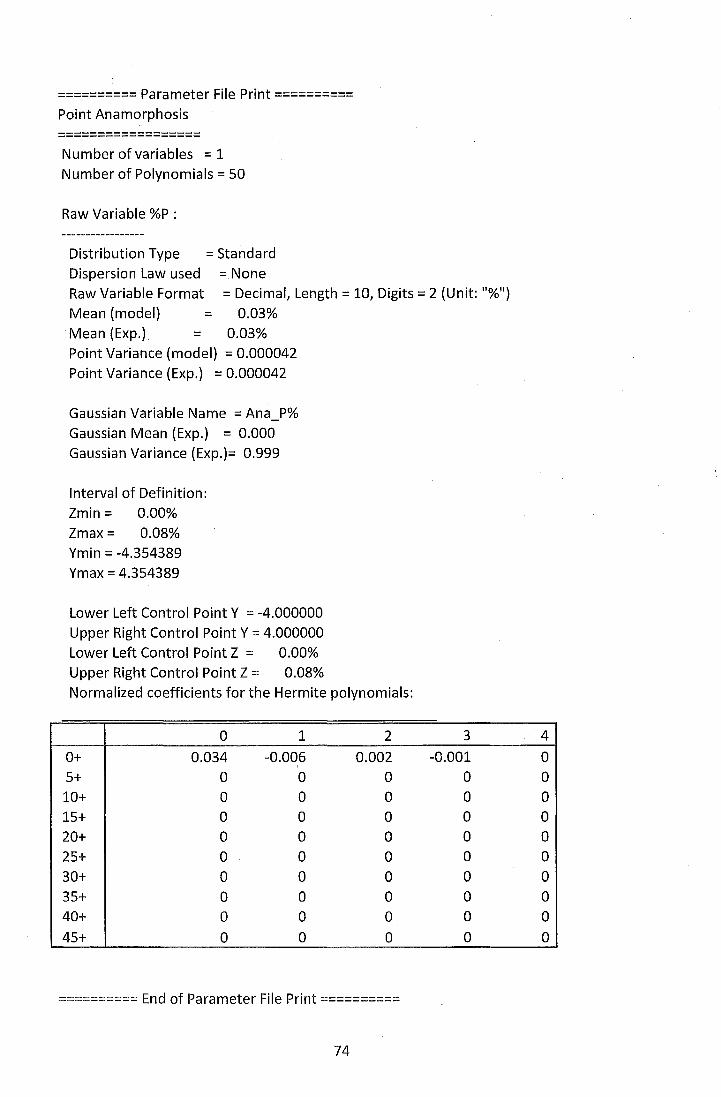
========== Parameter File Print========== Point Anamorphosis
================== Number of variables = 1 Number of Polynomials= 50
Raw Variable %P :
Distribution Type =Standard Dispersion law used = None Raw Variable Format = Decimal, Length = 10, Digits = 2 (Unit: "%") Mean (model) = 0.03% Mean (Exp.) = 0.03% Point Variance (model) = 0.000042 Point Variance (Exp.) = 0.000042
Gaussian Variable Name = Ana_P% Gaussian Mean (Exp.) = 0.000 Gaussian Variance (Exp.)= 0.999
Interval of Definition: Zmin = 0.00% Zmax = 0.08% Ymin = -4.354389 Ymax = 4.354389
lower left Control PointY = -4.000000 Upper Right Control PointY= 4.000000 lower left Control Point Z = 0.00% Upper Right Control Point Z = 0.08% Normalized coefficients for the Hermite polynomials:
0 1 2
0+ 0.034 -0.006 0.002
5+ 0 0 0 10+ 0 0 0 15+ 0 0 0 20+ 0 0 0 25+ 0 0 0
30+ 0 0 0 35+ 0 0 0 40+ 0 0 0
45+ 0 0 0
========== End of Parameter File Print==========
74
3
-0.001 0 0 0 0 0
0 0 0
0
4
0 0 0 0 0 0 0 0 0
0

========== Parameter File Print========== Point Anamorphosis
================== Number of variables = 1 Number of Polynomials= 40
Raw Variable %5 :
Distribution Type =Standard Dispersion Law used = None Raw Variable Format = Decimal, Length = 10, Digits = 2 (Unit: "%") Mean (model) = 0.01% Mean (Exp.) = 0.01% Point Variance (model) = 0.000007 Point Variance (Exp.) = 0.000007
Gaussian Variable Name = Ana_S% Gaussian Mean (Exp.) = 0.000 Gaussian Variance (Exp.)= 0.999
Interval of Definition: Zmin = 0.00% Zmax = 0.02% Ymin = -4.742394 Ymax = 4.354389
Lower Left Control Point Y = -4.000000 Upper Right Control PointY= 4.000000 Lower Left Control Point Z = 0.00% Upper Right Control Point Z = 0.02% Normalized coefficients for the Hermite polynomials:
0 1 2
0+ 0.007 -0.003 0.001 5+ 0 0 0 10+ 0 0 0 15+ 0 0 0 20+ 0 0 0 25+ 0 0 0 30+ 0 0 0
35+ 0 0 0
========== End of Parameter File Print==========
75
3
0 0 0 0 0 0 0
0
4
0 0 0 0 0 0 0
0

========== Parameter File Print========== Point Anamorphosis
================== Number of variables = 1 Number of Polynomials= 40
Raw Variable %Si02 :
Distribution Type =Standard Dispersion Law used = None Raw Variable Format = Decimal, Length = 10, Digits= 2 (Unit: "%") Mean (model) = 7.13% Mean (Exp.) = 7.13% Point Variance (model) = 3.066877 Point Variance (Exp.) = 3.068877
Gaussian Variable Name = Ana_Si02% Gaussian Mean (Exp.) = 0.000 Gaussian Variance (Exp.)= 0.999
Interval of Definition: Zmin = 3.00% Zmax = 22.00% Ymin = -4.451214 Ymax = 4.645223
Lower Left Control Point Y = -4.000000 Upper Right Control PointY= 4.000000 Lower Left Control Point Z = 3.00% Upper Right Control Point Z = 22.00% Normalized coefficients for the Hermite polynomials:
0 1 2
0+ 7.131 -1.707 0.346 5+ -0.013 -0.035 0.029 10+ 0.005 -0.001 0.007 15+ 0.01 0.005 -0.01 20+ -0.008 0 0.007 25+ 0.007 -0.001 -0.006 30+ -0.006 0 0.005
35+ 0.004 0.001 -0.003
========== End of Parameter File Print==========
76
3 4
-0.137 0.106 -0.009 -0.007 -0.004 -0.01 0.003 0.006
-0.005 -0.004 0.004 0.003
-0.002 -0.003
0.001 0.002

========== Parameter File Print ========== Point Anamorphosis
================== Number of variables = 1 Number of Polynomials= 50
Raw Variable %Ti02 :
Distribution Type = Standard Dispersion Law used = None Raw Variable Format = Decimal, Length = 10, Digits= 2 (Unit: "%") Mean (model) = 0.11% Mean (Exp.) = 0.11% Point Variance (model) = 0.010400 Point Variance (Exp.) = 0.010412
Gaussian Variable Name = Ana_Ti02% Gaussian Mean (Exp.) = 0.000 Gaussian Variance (Exp.)= 0.999
Interval of Definition: Zmin = 0.00% Zmax = 0.88% Ymin = -4.306025 Ymax = 4.402786
Lower Left Control Point Y = -4.000000 Upper Right Control PointY= 4.000000 Lower Left Control Point Z = 0.00% Upper Right Control Point Z = 0.88% Normalized coefficients for the Hermite polynomials:
0 1 2
0+ 0.106 -0.085 0.051 5+ 0.007 -0.005 0 10+ 0 0.001 -0.001 15+ 0 0 0 20+ 0 0 0 25+ 0 0 0 30+ 0 0 0 35+ 0 0 0 40+ 0 0 0
45+ 0 0 0
========== End of Parameter File Print==========
77
3 4
-0.02 0 0.003 -0.002
0 0.001 0 0 0 0 0 0 0 0 0 0 0 0
0 0

Appendix 3 - Average Distances, Experimental
Semivariogram Matrices and Eigenvalues Table Al- The average distance, experimental semivariogram matrices using the normal scores and corresponding eigenvalues.
Average Distance Matrix Eigenvalues
Al203 Fe Si02 Ti02 LOI
AI20 3 0.8517 -0.6108 0.3467 0.7624 0.5083 0.0188
6.959 Fe -0.6108 0.7558 -0.6458 -0.5632 -0.3632 0.04
Si02 0.3467 -0.6458 0.7283 0.3322 0.0739 0.3217
Ti02 0.7624 -0.5632 0.3322 0.7568 0.4439 0.7916
LOI 0.5083 -0.3632 0.0739 0.4439 0.782 2.7024
AhOl Fe Si02 Ti02 LOI
AI20 3 0.9073 -0.6464 0.3615 0.8164 0.5184 0.0222
16.721 Fe -0.6464 0.8083 -0.6841 -0.5992 -0.369 0.0431
Si02 0.3615 -0.6841 0.7652 0.3476 0.0718 0.3577
Ti02 0.8164 -0.5992 0.3476 0.8147 0.4544 0.8385
LOI 0.5184 -0.369 0.0718 0.4544 0.8145 2.8486
Al203 Fe Si02 Ti02 LOI
AI20 3 0.9416 -0.6642 0.3649 0.8559 0.5165 0.0252
30.822 Fe -0.6642 0.8345 -0.7007 -0.6238 -0.3656 0.0489
Si02 0.3649 -0.7007 0.784 0.3563 0.0626 0.3959
Ti02 0.8559 -0.6238 0.3563 0.8722 0.449 0.8709
LOI 0.5165 -0.3656 0.0626 0.449 0.8382 2.9296
Al203 Fe Si02 Ti02 LOI
Al203 0.9719 -0.6753 0.3637 0.8859 0.5243 0.0264
45.331 Fe -0.6753 0.8512 -0.7134 -0.6367 -0.3607 0.0548
Si02 0.3637 -0.7134 0.7998 0.3578 0.0499 0.4208
Ti02 0.8859 -0.6367 0.3578 0.9154 0.4486 0.9099
LOI 0.5243 -0.3607 0.0499 0.4486 0.8616 2.988
Al203 Fe Si02 Ti02 LOI
Al203 0.9941 -0.6928 0.3775 0.9137 0.5333 0.0271
60.155 Fe -0.6928 0.8779 -0.7367 -0.6559 -0.3732 0.0577
Si02 0.3775 -0.7367 0.8221 0.3748 0.0551 0.4569
Ti02 0.9137 -0.6559 0.3748 0.9578 0.4462 0.9317
LOI 0.5333 -0.3732 0.0551 0.4462 0.8991 3.0779
78

Table Al continued- The average distance, experimental semivariogram matrices using the normal scores and corresponding eigenvalues.
AhO"l Fe Si02 Ti02 LOI
Al20 3 1.0116 -0.7026 0.3821 0.9323 0.5407 0.0271 75.159 Fe -0.7026 0.8968 -0.7546 -0.6651 -0.3804 0.0595
Si02 0.3821 -0.7546 0.8404 0.3804 0.0584 0.487
Ti02 0.9323 -0.6651 0.3804 0.9834 0.4441 0.955
LOI 0.5407 -0.3804 0.0584 0.4441 0.9297 3.1333
AhOJ Fe Si02 Ti02 LOI
Al20 3 1.0163 -0.6996 0.3805 0.9387 0.543 0.0272
90.052 Fe -0.6996 0.8976 -0.7602 -0.6621 -0.383 0.0611
Si02 0.3805 -0.7602 0.8491 0.3796 0.0626 0.5159
Ti02 0.9387 -0.6621 0.3796 0.9984 0.4357 0.9674
LOI 0.543 -0.383 0.0626 0.4357 0.9536 3.1434
AhOJ Fe Si02 Ti02 LOI
Al20 3 1.0223 -0.7013 0.3836 0.9473 0.5453 0.0267
104.986 Fe -0.7013 0.9099 -0.7809 -0.6665 -0.384 0.063
Si02 0.3836 -0.7809 0.8772 0.3859 0.0652 0.536
Ti02 0.9473 -0.6665 0.3859 1.0158 0.432 0.9914
LOI 0.5453 -0.384 0.0652 0.432 0.9677 3.1758
AhOJ Fe Si02 Ti02 LOI
Al20 3 1.0201 -0.7085 0.393 0.9437 0.5445 0.0269
120.005 Fe -0.7085 0.9268 -0.802 -0.6722 -0.389 0.0638
Si02 0.393 -0.802 0.9035 0.3954 0.0722 0.5551
Ti02 0.9437 -0.6722 0.3954 1.0151 0.421 1.0047
LOI 0.5445 -0.389 0.0722 0.421 0.9875 3.2025
AhOJ Fe Si02 Ti02 LOI
Al20 3 1.0314 -0.7222 0.4063 0.9518 0.5556 0.0268
135.021 Fe -0.7222 0.9402 -0.815 -0.6851 -0.3995 0.0641
Si02 0.4063 -0.815 0.9156 0.4086 0.0807 0.5591
Ti02 0.9518 -0.6851 0.4086 1.0233 0.4243 1.0069
LOI 0.5556 -0.3995 0.0807 0.4243 1.0026 3.2562
Al203 Fe Si02 Ti02 LOI
Al20 3 1.0275 -0.7256 0.4122 0.9445 0.5469 0.0264
149.904 Fe -0.7256 0.9514 -0.8276 -0.6883 -0.4005 0.0648
Si02 0.4122 -0.8276 0.9272 0.4164 0.087 0.5758
Ti02 0.9445 -0.6883 0.4164 1.017 0.4056 1.005
LOI 0.5469 -0.4005 0.087 0.4056 1.0097 3.2607
79

Table Al continued- The average distance, experimental semivariogram matrices using the normal scores and corresponding eigenvalues.
Al203 Fe s'io2 Ti02 LOI
Al203 1.0312 -0.7219 0.4127 0.9387 0.5472 0.0256
164.941 Fe -0.7219 0.9497 -0.8343 -0.6832 -0.3988 0.0653
Si02 0.4127 -0.8343 0.9372 0.418 0.0918 0.5829
Ti02 0.9387 -0.6832 0.418 1.0064 0.3944 1.0059
LOI 0.5472 -0.3988 0.0918 0.3944 1.008 3.2529
AI20 3 Fe Si02 Ti02 LOI
AI20 3 1.0228 -0.7128 0.403 0.9254 0.54 0.0254
179.968 Fe -0.7128 0.9575 -0.8464 -0.6765 -0.3968 0.0677
Si02 0.403 -0.8464 0.9537 0.4136 0.0943 0.6091
Ti02 0.9254 -0.6765 0.4136 0.9985 0.3726 1.0195
LOI 0.54 -0.3968 0.0943 0.3726 1.0186 3.2295
AhO~ Fe Si02 Ti02 LOI
Al203 1.0297 -0.716 0.4067 0.9269 0.5411 0.0255
194.881 Fe -0.716 0.9671 -0.8579 -0.6764 -0.4069 0.071
Si02 0.4067 -0.8579 0.9665 0.4149 0.1081 0.6289
Ti02 0.9269 -0.6764 0.4149 1.0045 0.3656 1.0142
LOI 0.5411 -0.4069 0.1081 0.3656 1.0226 3.2508
AhO~ Fe Si02 Ti02 LOI
Al203 1.0196 -0.7049 0.3985 0.9197 0.5273 0.0262
209.877 Fe -0.7049 0.9753 -0.8704 -0.6671 -0.4137 0.0722
Si02 0.3985 -0.8704 0.984 0.4089 0.1208 0.6653
Ti02 0.9197 -0.6671 0.4089 1.0052 0.3468 1.0128
LOI 0.5273 -0.4137 0.1208 0.3468 1.0266 3.2342
80

Table A2- The average distance, experimental semivariogram matrices using the standardised and corresponding eigenvalues.
Avera~eLa~ Matrix Ei~envalues
Al203 Fe Si02 Ti02 LOI
Al203 0.8678 -0.7567 0.4924 0.7814 0.4993 0.0045 6.959 Fe -0.7567 0.8199 -0.6951 -0.6676 -0.3898 0.0363
Si02 0.4924 -0.6951 0.7645 0.4234 0.0984 0.2661
Ti02 0.7814 -0.6676 0.4234 0.7797 0.4296 0.7292
LOI 0.4993 -0.3898 0.0984 0.4296 0.7858 2.9816
AhOl Fe Si02 Ti02 LOI
AI20 3 0.8951 -0.7778 0.5033 0.8127 0.4962 0.0059
16.721 Fe -0.7778 0.8492 -0.7184 -0.6877 -0.3948 0.0393
Si02 0.5033 -0.7184 0.7908 0.4309 0.0986 0.3092
Ti02 0.8127 -0.6877 0.4309 0.8229 0.4232 0.76
LOI 0.4962 -0.3948 0.0986 0.4232 0.8211 3.0649
AhOl Fe Si02 Ti02 LOI
Al203 0.8865 -0.7614 0.4835 0.8128 0.4794 0.007
30.822 Fe -0.7614 0.8397 -0.7115 -0.678 -0.3825 0.0436
Si02 0.4835 -0.7115 0.7941 0.416 0.0856 0.3479
Ti02 0.8128 -0.678 0.416 0.8425 0.4025 0.7851
LOI 0.4794 -0.3825 0.0856 0.4025 0.8399 3.0191
AI20 3 Fe Si02 Ti02 LOI
AI20 3 0.8807 -0.7511 0.4693 0.8108 0.478 0.0077
45.331 Fe -0.7511 0.8353 -0.7074 -0.6712 -0.3776 0.0469
Si02 0.4693 -0.7074 0.7951 0.4064 0.0751 0.3672
Ti02 0.8108 -0.6712 0.4064 0.8534 0.3941 0.8088
LOI 0.478 -0.3776 0.0751 0.3941 0.8596 2.9935
AbOl Fe Si02 Ti02 LOI
Al203 0.917 -0.7776 0.4838 0.8477 0.4914 0.0078
60.155 Fe -0.7776 0.8638 -0.7291 -0.6968 -0.3928 0.0496
Si02 0.4838 -0.7291 0.8155 0.4229 0.0811 0.3997
Ti02 0.8477 -0.6968 0.4229 0.8996 0.3953 0.8334
LOI 0.4914 -0.3928 0.0811 0.3953 0.8989 3.1042
AhOl Fe Si02 Ti02 LOI
Al203 0.9524 -0.8032 0.4959 0.8835 0.5068 0.0077
75.159 Fe -0.8032 0.8882 -0.7457 -0.7233 -0.4089 0.0517
Si02 0.4959 -0.7457 0.831 0.4376 0.0881 0.4256
Ti02 0.8835 -0.7233 0.4376 0.9435 0.3999 0.8514
LOI 0.5068 -0.4089 0.0881 0.3999 0.9315 3.21
81

Table A2 continues- The average distance, experimental semivariogram matrices using the standardised and corresponding eigenvalues.
Al203 Fe Si02 Ti02 LOI
Al203 0.9694 -0.812 0.4982 0.902 0.5157 0.0076
90.052 Fe -0.812 0.8978 -0.7548 -0.7317 -0.4193 0.0523
Si02 0.4982 -0.7548 0.8436 0.4395 0.0942 0.4527
Ti02 0.902 -0.7317 0.4395 0.9679 0.3996 0.8664
LOI 0.5157 -0.4193 0.0942 0.3996 0.9582 3.2578
Ah_01 Fe Si02 Ti02 LOI
Al203 0.9855 -0.8283 0.513 0.9191 0.5203 0.0076
104.986 Fe -0.8283 0.9234 -0.7842 -0.7473 -0.426 0.054
Si02 0.513 -0.7842 0.88 0.4535 0.0991 0.473
Ti02 0.9191 -0.7473 0.4535 0.9917 0.3992 0.8866
LOI 0.5203 -0.426 0.0991 0.3992 0.973 3.3323
Ah01 Fe Si02 Ti02 LOI
AI20 3 1.0235 -0.8623 0.5385 0.9495 0.5306 0.0077
120.005 Fe -0.8623 0.9622 -0.8201 -0.7731 -0.4386 0.0562
Si02 0.5385 -0.8201 0.9184 0.4724 0.1091 0.4977
Ti02 0.9495 -0.7731 0.4724 1.0216 0.3995 0.9071
LOI 0.5306 -0.4386 0.1091 0.3995 0.9966 3.4537
Al201 Fe Si02 Ti02 LOI
Ai20 3 1.0458 -0.89 0.562 0.9628 0.5479 0.0077
135.021 Fe -0.89 0.995 -0.8484 -0.7929 -0.4555 0.0581
Si02 0.562 -0.8484 0.9434 0.4905 0.1218 0.4971
Ti02 0.9628 -0.7929 0.4905 1.0323 0.4098 0.9124
LOI 0.5479 -0.4555 0.1218 0.4098 1.0088 3.5501
Al201 Fe Si02 Ti02 LOI
AI20 3 1.0238 -0.8783 0.5616 0.9392 0.5349 0.0077
149.904 Fe -0.8783 0.9926 -0.8548 -0.7819 -0.4491 0.0614
Si02 0.5616 -0.8548 0.9536 0.4918 0.1245 0.5016
Ti02 0.9392 -0.7819 0.4918 1.0156 0.3922 0.9117
LOI 0.5349 -0.4491 0.1245 0.3922 1.007 3.5102
Ah_03 Fe Si02 Ti02 LOI
AI20 3 1.0364 -0.8917 0.5753 0.9443 0.5382 0.0075
164.941 Fe -0.8917 1.0111 -0.8761 -0.79 -0.4526 0.0655
Si02 0.5753 -0.8761 0.9772 0.5027 0.131 0.5105
Ti02 0.9443 -0.79 0.5027 1.0263 0.386 0.9116
LOI 0.5382 -0.4526 0.131 0.386 1.002 3.5579
82

Table A2 continued- The average distance, experimental semivariogram matrices using the standardised and corresponding eigenvalues.
Al203 Fe Si02 Ti02 LOI
Al203 1.0284 -0.8837 0.5693 0.9307 0.5313 0.0075
179.968 Fe -0.8837 1.0109 -0.8821 -0.7804 -0.4504 0.0704
Si02 0.5693 -0.8821 0.9905 0.4982 0.1345 0.5308
Ti02 0.9307 -0.7804 0.4982 1.0221 0.3665 0.9133
LOI 0.5313 -0.4504 0.1345 0.3665 1.0025 3.5323
Ah01 Fe Si02 Ti02 LOI
Al203 1.0581 -0.9078 0.5867 0.9522 0.5393 0.0075
194.881 Fe -0.9078 1.0374 -0.9053 -0.7969 -0.465 0.0771
Si02 0.5867 -0.9053 1.0122 0.5088 0.1512 0.5548
Ti02 0.9522 -0.7969 0.5088 1.0537 0.3676 0.9073
LOI 0.5393 -0.465 0.1512 0.3676 1.0066 3.6213
Al203 Fe Si02 Ti02 LOI
Al203 1.0559 -0.9007 0.5804 0.9486 0.5301 0.0076
209.877 Fe -0.9007 1.0368 -0.9086 -0.7897 -0.4698 0.0843
Si02 0.5804 -0.9086 1.0193 0.5048 0.1633 0.5911
Ti02 0.9486 -0.7897 0.5048 1.0695 0.3472 0.8981
LOI 0.5301 -0.4698 0.1633 0.3472 1.0093 3.6097
83

Appendix 4 - Scatter Plots and Correlation Coefficients of
Factors
4.1 PCA Factors using Normal Scores
Scatter plots
~~ ~I • S
" ~~ 'f:_
1 ·0.5
+ ••
Correlation Matrix:
VARIABLES F1 PCA NS
F1 PCA NS 1 - -
F2 PCA NS 0 - -
F3 PCA NS 0 - -
F4 PCA NS 0 - -
F5 PCA NS 0
0
FlPCA IIS
F2 PCA NS
0
1
0
0
0
9 -, ~I
=,
~I
+
*
...
. ~:~-" .. :~ + +
+ t
F3 PCA NS F4 PCA NS
0 0
0 0
1 0
0 1
0 0
84
F5 PCA NS
0
0
0
0
1

4.2 PCA Factors usin.g Standardised Variables
Scatter plots
~:
~I ~I
~:
~:
+ t;:..,. +
+ +
+ + + +
+ + tl-+ + + ++ +
Correlation Matrix:
VARIABLES F1 PCA S
F1 PCA S 1 - -
F2 PCA S 0 - -
F3 PCA S 0 - -
F4 PCA S 0 - -
F5 PCA S 0
~:
~:
~:
F2 PCA S
0
1
0
0
0
+ + + +
F3 PCA S
0
0
1
0
0
85
~:
~:
~:
F4 PCA S
0
0
0
1
0
++
++ +
F5 PCA S
0
0
0
0
1

4.3 MAF Factors using Normal Scores
Scatter plots
~I ~ I
~I ~ I
~I
~I
~ I
~I
Correlation Matrix: F1 PCA
VARIABLES NS
F1 PCA NS 1 - -
F2 PCA NS 0 - -
F3 PCA NS 0 - -
F4 PCA NS 0 - -
F5 PCA NS 0
+.,.
F2 PCA NS
0
1
0
0
0
86
+ + +
F3 PCA NS
0
0
1
0
0
~I
~I
~I
~I
F4 PCA NS
0
0
0
1
0
+ + +
+ + +
F5 PCA NS
0
0
0
0
1

4.4 MAF Factors usi~g Standardised Variables
Scatter plots
:
Correlation Matrix:
VARIABLES F1 MAF S
F1 MAF S 1 - -
F2 MAF S 0 - -
F3 MAF S 0 - -
F4 MAF S 0 - -
F5 MAF S 0
+ +
F2 MAF S
0 1
0
0
0
87
++
-4 -3 -2 -1 0
F3 MAF S
F3 MAF S F4 MAF S
0 0
0 0
1 0
0 1
0 0
+ +
++
F5 MAF S
0 0
0
0
1

4.5 ACDC Factors using J~ormal Scores
Scatter plots
Correlation Matrix:
VARIABLES
F1 ACDC NS -
F2 ACDC NS - -
F3 ACDC NS - -
F4 ACDC NS - -
F5 ACDC NS
·• +
+ +
F1 ACDC NS
1
0
-0.01
-0.02
-0.01
+ .
F2 ACDC -NS
0
1
-0.05
0.03
-0.08
+ +
F3 ACDC -
NS
-0.01
-0.05
1
0
0.02
88
F4 ACDC NS
-0.02
0.03
0
1
-0.05
+ +
\ +
F5 ACDC NS
-0.01
-0.08
0.02
-0.05
1

4.6 ACDC Factors u~ing Standardised Variables
Scatter plots
+ +++4 + + +
-I¢
~I ++ "' I ~I ~I
ii-~I ;I
... + ++ + +++ / }" + + +
fl ACDC S fl ACDC S F l ACDC S -
+ + ++
++ + + "'++
++
~I ~I ~I ;I ~I ~I
++
+ ++
+ +
+ + +_, +
Fl ACDC s - F2 ACDC S F2 ACDC S
+:·+ +
+ + + +
~I ~I :I s ;I
+ + ;I ~I
+ +
++ +
F2 ACDC S F3 ACDC S F3 ACDC S -
. + ++-t
:I s ;I
Correlation Matrix:
VARIABLES F1 ACDC s F2 ACDC s F3 ACDC s F4 ACDC s F5 ACDC s F1 ACDC S 1 0.01 0 -0.06 0.02
-
F2 ACDC S 0.01 1 -0.01 -0.03 0.02 - -
F3 ACDC S 0 -0.01 1 0.01 -0.02 - -
F4 ACDC S -0.06 -0.03 0.01 1 -0.03 - -
F5 ACDC S 0.02 0.02 -0.02 -0.03 1
89

4.7 ACDC Factors using Normal Scores and Matrix AoNs
Scatter plots
~I
~I
++ +
CorrelationMatrix:
VARIABLES
FI ACDC NS+AO - -
F2 ACDC NS+ AO - -
F3 ACDC NS+ AO - -
F4 ACDC NS+AO - -
F5 ACDC NS+ AO - -
++
FI ACDC -NS+AO
1
-0.03
-0.05
0.04
0.02
F2 ACDC NS - -+AO
-0.03
1
0.02
-O.I
0
90
~I
~I
5 .
F3 ACDC NS - -+AO
-0.05
0.02
I
-0.07
0
- 4 · l 0 l 2 3 "
+ +
Fl_Acoc_i1s
F4 ACDC NS - -+AO
0.04
-O.I
-0.07
I
-0.05
F5 ACDC NS - -+AO
0.02
0
0
-0.05
1

4.8 ACDC Factors us.ing Standardised Variables and Matrix
Aost Scatter plots
++ +-+:..+ ..
+
~
· "· ~~ + ...
"' + + +
++ ,.<f'll- ....
~+ + +"'
f- T+ +~ + +++
15
Fl ACDC S Pl ACOC S Fl ACDC S
+ .. +
' ,:j: + ~ ....
il w w I
*-;. ++ ~ ~ ++ +
I +T.o. + l!: :;: ;!
4 +
Pl ACOC S P2 ACDC S F2 ACDC S
++ + "' +
+ +
: I w
:I
~ I
~ ~ I
l!: ;! l!:
+ ++ ...
P2 ACDC S FJ ACDC S F3 ACDC S
Correlation matrix:
F1 ACDC F2 ACDC F3 ACDC S F4 ACDC S F5 ACDC S - - - - - - - -VARJABLES S+AO S+AO +AO +AO +AO
F1 ACDC S +AO 1 -0.01 -0.04 -0.05 -0.02 - -
F2 ACDC S +AO -0.01 1 0.09 -0.06 0.04 - -F3 ACDC S +AO -0.04 0.09 1 0.04 0.11 - -
F4 ACDC S +AO -0.05 -0.06 0.04 1 -0.03 - -
F5 ACDC S +AO -0.02 0.04 0.11 -0.03 1
91

Appendix 5- Experimental Cross Semivariograms and Spatial
Decorrelation Plots of the ACDC Factors
ACDC using Normal scores, weight vector [1 1 1 1 1 1 1 1 1 1 1 1·1 1 1]
0.9
0.8 -4-AC1-AC2 --+-ACl-ACJ
0.7 -4- AC2-AC3 -t-- AC1-AC4
-4- AC2-AC4 0.6
---+--- AC 1-AC5 0.5 -4- AC2-ACS --+- ACJ-ACS 0.4 ~AC4-AC5
0.3
oL_----~----~----~~~~~ 0 50 100 200
Lag h (m)
ACDC using Normal scores, weight vector [1 1 1 1 1 1 1 1 1 1 1 1 1 1 0]
-+- AC2-AC3
-t- AC1-AC4
-+- AC2-AC4 AC3-AC4
100 120 140 160 180 200 Lagh(m)
0.9
0.8
0.7
_Q 0.6
'" w ~ 0.5
0 0.4
0.3
ACDC using Normal scores, weight vector [1 1 1 1 1 1 1 1 1 1 1 1 1 0 0]
0.9
-+- AC1-AC2 -t-- AC1-AC3 0.8
-t-- AC2-AC3
-I--- AC1-AC4 0.7
-+- AC2-AC4 AC3-AC4 0.6
---+- AC2-AC5 0.5 ~AC3-AC5
---+- AC4-AC5 0.4
0.3
Lagh(m)
92

ACDC using Normal scores, weight vector [1 1 1 1 1 1 1 1 1 1 1 1 0 0 0]
-+- AC1 -AC2 --+- AC1-AC3
--+- AC2-AC4
AC3-AC4 --+-- AC1-ACS --t- AC2-ACS -+- AC3-AC5 -+- AC4-AC5
0.9
0.8
0.7
_§ 0.6 iii 1 05
0 0.4
0.3
0.1
QL-----~------~----~~------~ 0 50 100 150 200
lag h (m)
ACDC using Normal scores, weight vector [1 1 1 1 1 1 1 1 1 1 1 0 0 0 0]
0. 1
-O. 1 o'.'---:20'::-----='4o=--~so=---:':so,--1~oo=--1~20=--1""4o::--1-':-:60,------,1-':-:B0------=200':-:
Lagh(m)
-+-AC1-AC2 -+- AC 1-AC3 -+- AC2-AC3 -+- AC 1-AC4 -+- AC2-AC4
AC3-AC4 -+- AC 1-AC5 ----.- AC2-AC5 -+- AC3-AC5 -+- AC4-AC5
0.9
0.8
0.7
~ 0.6 Qj
~ 0.5
0 0.4
0.3
0.2
lag h (m)
ACDC using Normal scores, weight vector [1 1 1 1 1 1 1 1 1 1 0 0 0 0 0]
0.9
--+- AC1-AC2 0.8 -.-- AC1-AC3 --+- AC2-AC3 0.7 ->-- AC1-AC4
--+- AC2-AC4 AC3-AC4
0.6
-;- AC1-AC5
--+- AC2-AC5 0.5
--+- AC3-AC5 --+- AC4-AC5 0.4
0.3
0.2
-0.2 0. 1
.o.25 oL_ _____ so:':-------1~oo:------~, so-=--------:"200~ 0 0
Lagh (m) lag h (m)
93

ACDC using Normal scores, weight vector [1 1 1 1 1 1 1 1 1 0 0 0 0 0 0]
.0.25
100 Lagh(m)
150
-+- AC 1-AC2 -+- AC 1-AC3 -+- AC2-Ac:J --t-- AC 1-AC4
-+- AC2-AC4 AC3-AC4
-+-AC1-AC5 -+- AC2-ACS _._ ACJ-ACS -+- AC4-ACS
200
0.9
0.8
0.7
c 0.6 0
iii
1 0.5
~ 0.4
0.3
0.2
0.1
ACDC using Normal scores, weight vector [1 1 1 1 1 1 1 1 0 0 0 0 0 0 0]
-0.25
50 100 Lagh(m)
150 200
0.9 -+- AC1-AC2 --AC1-AC3 0.8 -+- AC2-AC3
--+- AC1-AC4 0.7 -+- AC2-AC4
AC3-AC4 0 0.6 -+-AC1-AC5 "' -+- AC2-AC5 1 0.5 -+- Ac:J.ACS -+- AC4-AC5 0 0.4
0.3
0.1
Lag h (m)
ACDC using Normal scores, weight vector [1 1 1 1 1 1 1 0 0 0 0 0 0 0 0]
0.15
0.1
-0 1
-0 15L_ ____ ~50 _______ 1 00~----~150~--~2~00
Lag h (m)
-+- AC1-AC2 --AC1-AC3 -+- AC2-AC3 -+- AC1-AC4 -+- AC2-AC4
AC3-AC4 -+-AC1-AC5 -+- AC2-AC5 -+- AC3-AC5 -+- AC4-AC5
0.9
0.8
0.7
0.6
0.5
0.4
94
200

ACDC using Normal scores, weight vector [1 1 1 1 1 1 0 0 0 0 0 0 0 0 0]
ACDC using Normal scores, weight vector [1 1 1 1 1 0 0 0 0 0 0 0 0 0 0]
0.9
0.4 --+- AC1-AC2 0.8 _...__ AC1 -AC3
0.3 --+- AC2-AC3 0.7 -~ AC1 -AC4
0.2
--+- AC2-AC4 c 0.6 AC3-AC4
0
ro -+-AC1-ACS 1 0.5 --+- AC2-ACS --+- AC3-ACS --+- AC4-ACS
0 0.4
0.3
0.2
0.1
Lag h {m)
ACDC using Normal scores, weight vector [1 1 1 1 0 0 0 0 0 0 0 0 0 0 0]
-+- AC1 -AC2 0.9
0.1 -+- AC1 -ACJ 0.8 -+- AC2-ACJ
-- AC1-AC4 0.7
-+- AC2-AC4 AC~AC4
0.6 -+- AC1-AC5 -+- AC2-AC5
0.5 -~ AC~ACS
-+- AC4-AC5 0.4
.0.2
50 100 150 200 Lag h(m) Lag h {m)
95

ACDC using Normal scores, weight vector [1 1 1 0 0 0 0 0 0 0 0 0 0 0 0]
0.2
0.15
-0.15
-0.2
.o.25':----::so:-----:1-::oo------:-!1so=---20::-o::
Lag h (m)
-+- AC1-AC2 _.,__ AC1-AC3 -+- AC2-AC3 -+- AC1 -AC4 -+- AC2-AC4
AC3-AC4 --+- AC1 -AC5 -+- AC2-AC5 -+- AC3-AC5 -+- AC4-AC5
0.9
0.8
0.7
0 0.6 1a
~ 0.5 hl
. 0 0.4
0.3
Lag h (m)
ACDC using Normal scores, weight vector [1 1 0 0 0 0 0 0 0 0 0 0 0 0 0]
-+-- AC1-AC2 0.9 -+-- AC1 -AC3 -+-- AC2-AC3 0.8 --+- AC1-AC4 -+-- AC2-AC4 0.7
AC3-AC4 -+-- AC1-AC5 .Q 0.6 -+-- AC2-ACS iii
;:/ a;
-+-- AC3-AC5 ~ 0.5 -+-- AC4-AC5
0 0.4
0.3 ./if 0.2 /
/'
/Jil 0.1 -~)"
0 0 50 100 150
Lag h (m) Lag h (m)
ACDC using Normal scores, weight vector [1 0 0 0 0 0 0 0 0 0 0 0 0 0 0]
-.;..- AC1 -AC2 -!-- AC1-AC3 --+- AC2-AC3 0.9
-+- AC1 -AC4
--+- AC2-AC4 0.8
AC3-AC4 0.7 -.;..- AC1 -ACS
--+- AC2-ACS 0.6 --+- AC3-ACS --+- AC4-ACS 0.5
0.4
-0.4 0.3
-0.5
50 100 150 200 150 Lag h (m) Lag h (m)
96
200
200

ACDC using Normal scores and AoNs matrix, weight vector [1 1 1 1 1 1 1 1 1 1 1 1 1 1 1]
-+- AC1-AC2 -<>-- AC1-AC3
-+- AC2-AC3 --AC1-AC4 --AC2-AC4
AC3-AC4 -+- AC1-AC5 -+- AC2-AC5 -t-- AC3-AC5 -+- AC4-AC5
Lag h (m)
0.9
0.8
0.7
_Q 0.6 1ij Qj
~ 0.5 g 0 0.4
0.3
0 . 2f~ .
0.1 7""""-'?,~~ 0 ~'"-= -,.-
0 50 100 150 200 Lag h (m)
ACDC using Normal scores and AoNs matrix, weight vector [1 1 1 1 1 1 1 1 1 1 1 1 1 1 0]
0.9
--t-- AC 1-AC2 0.8
_...._ AC1-AC3
-+- AC2-AC3 0.7 -+- AC1-AC4 -+- AC2-AC4 0 0.6
AC3-AC4 ~ -+- AC1 -ACS ~ 0.5 -+- AC2-AC5 g --AC3-AC5 0 0.4 -+- AC4-ACS
0.3
0.2
0.1
0 0 50 100 150 200
Lag h (m)
ACDC using Normal scores and AoNs matrix, weight vector [1 1 1 1 1 1 1 1 1 1 1 1 1 0 0]
0.9
-+- AC1-AC2 --.-- AC1-AC3
0.8
-+- AC2-AC3 0.7
- t - AC1-AC4
-+- AC2-AC4 0.6 AC3-AC4
-+-- AC1-AC5
-+-- AC2-AC5 0.5
--.-- AC3-ACS -+-- AC4-AC5 0.4
0.3
0.1
Lagh(m)
97

ACDC using Normal scores and AoNs matrix, weight vector [1 1 1 1 1 1 1 1 1 1 1 1 0 0 0]
0.06 ""'
0.04 I '\....-
-0.08
50 100 150 Lag h (m)
-+- AC1-AC2 0.9
-t- AC1-AC3 0.8
-+- AC2-AC3 - - AC1-AC4 0.7 -+- AC2-AC4
AC3-AC4 0 0.6
--+- AC1-AC5 ~ -+- AC2-AC5 1 0.5 --+- AC3-AC5 -+- AC4-AC5 0 0.4
0.3
0.2
Lag h (m)
ACDC using Normal scores and AoNs matrix, weight vector [1 1 1 1 1 1 1 1 1 1 1 0 0 0 0]
-+- AC1-AC2 0.9
---.- AC1 -AC3 0.8
-+- AC2-AC3 --<- AC1-AC4 0.7 -+- AC2-AC4
AC3-AC4 0 0.6 --+- AC 1-AC5 iij
-+- AC2-AC5 1 0.5 --+-- AC3-AC5 -+- AC4-AC5 0 0.4
0.3
0.2
Lag h (m)
ACDC using Normal scores and AoNs matrix, weight vector [1 1 1 1 1 1 1 1 1 1 0 0 0 0 0]
50 100 150 Lag h (m)
200
--+- AC1-AC2 --+- AC1-AC3 --+- AC2-AC3 -+- AC1-AC4
--+- AC2-AC4 AC3-AC4
---+-- AC1-AC5
--+- AC2-AC5 --+- AC3-AC5 --+- AC4-AC5
0.9
0.8
0.7
0.6
0.5
0.4
0.3
0.2
0.1
0 ~ 0 50 100
Lag h (m)
98

ACDC using Normal scores and AoNs matrix, weight vector [1 1 1 1 1 1 1 1 1 0 0 0 0 0 O]
-0.12
-0.14o.._ --~50:---1"-:00 _____ 150'c:---2,-c00.,-
Lagh(m)
-+- AC1-AC2 -.- AC1-AC3 -+- AC2-AC3 -.- AC1-AC4 -+- AC2-AC4
AC3-AC4 -+- AC1-AC5 --t- AC2-AC5 -.- AC3-AC5 -+- AC4-AC5
0.9
0.8
0.7
~ 0.6
1 0.5
0 0.4
0.3
0.2
Lag h (m)
ACDC using Normal scores and AoNs matrix, weight vector [1 1 1 1 1 1 1 1 0 0 0 0 0 0 0]
-+- AC1-AC2 0.9 __.__ AC1-AC3
-+- AC2-AC3 0.8
--+-- AC1-AC4
-+- AC2-AC4 0.7
AC3-AC4 c 0.6 --AC1-AC5
0
iii -+- AC2-AC5 1 0.5 -..- AC3-AC5 -+- AC4-AC5 0 0.4
0.3
0.2
0.1
Lag h (m)
ACDC using Normal scores and AoNs matrix, weight vector [1 1 1 1 1 1 1 0 0 0 0 0 0 0 0]
0.9
0.06 ~ -+- AC1-AC2 --AC1-AC3 0.8
-+- AC2-AC3 - ~- AC1-AC4 0.7
-+- AC2-AC4 AC3-AC4 0.6
-+- AC1-AC5 -+- AC2-AC5 0.5 --+-- AC3-AC5 -+- AC4-AC5 0.4
0.3
-0.1
-0.12 0.1
-0.14 0 50 100 150 200
Lagh (m) Lag h (m)
99

ACDC using Normal scores and AoNs matrix, weight vector [1 1 1 1 1 1 0 0 0 0 0 0 0 0 0]
0.06
0.04
-0.12 0:-----,so=----1.,.:-00::-----::150:::------::20::-o
lag h (m)
-+- AC1-AC2 -t- AC1-AC3 -+- AC2-AC3 -+-- AC1-AC4 -+- AC2-AC4
AC3-AC4 -+-- AC1-AC5 -+- AC2-AC5 -+-- AC3-AC5 -+- AC4-AC5
0.9
0.8
0.7
.~ 0.6 iii
1 0.5
0 0. 4
0.3
0.1
ACDC using Normal scores and AoNs matrix, weight vector [1 1 1 1 1 0 0 0 0 0 0 0 0 0 0]
0.05 -+-- AC1-AC2 -+-- AC1-AC3 -+-- AC2-AC3 0.9
-+-- AC1-AC4 -+-- AC2-AC4 0.8
AC3-AC4 0.7 -+-- AC1-AC5
--AC2-AC5 .§ 0.6 -+-- AC3-AC5 iii
~ Qj
-+-- AC4-AC5 5 0. 5 hl 0 0.4
0.3
0.2
0.1
-0. 1 0 50 100 150 200 0 sb
Lag h (m) Lag h (m)
ACDC using Normal scores and AoNs .matrix, weight vector [1 1 1 1 0 0 0 0 0 0 0 0 0 0 0]
0.04
0.02
o P* t ~ -ll.02
-ll.04
'2 -ll.06 -.:.
-ll.OB
-ll .1
-ll. 12
-{),14
-ll.16
50 100 Lagh (m)
150 200
0.9
-+- AC1-AC2 -t-AC1-AC3 0.8
-+- AC2-AC3 -+- AC1-AC4 0.7
-+- AC2-AC4 AC3-AC4 0.6
-+- AC1-AC5 -+- AC2-AC5 0. 5 -.- AC3-AC5 -+- AC4-AC5 0.4
0.3
0.2
0.1
0 0 50
100

ACDC using Normal scores and AoNs matrix, weight vector [1 1 1 0 0 0 0 0 0 0 0 0 o o OJ
0.,. -0.05
;;:. -0.1
-0.15
-0.2
50 100 150 200 Lag h (m)
-+- AC1-AC2 -+- AC1-AC3
-+- AC2-AC3 -+- AC1-AC4
-+- AC2-AC4 AC3-AC4
-+- AC1-AC5
-+- AC2-AC5 -+- AC3-AC5 -+- AC4-AC5
0.9
0.8
0.7
.§ 0.6 -ro a;
~ 0.5
0 0.4
0.3
Lag h (m)
ACDC using Normal scores and AoNs matrix, weight vector [1 1 0 0 0 0 0 0 0 0 0 0 0 0 OJ
0.9 -+- AC1 -AC2 -+- AC1 -AC3 0.8
0.1
-+- AC2-AC3 0.05 -+- AC1 -AC4 0.7
-+- AC2-AC4
~ -Q.1
AC3-AC4 0 0.6 -+-AC1-AC5 ~ -+- AC2-AC5 i 0.5 -+- AC3-AC5 -+- AC4-AC5 ~ 0.4
-0.05
-0.15 0.3
0.2 -0.2
0.1 -0.25
0 0
Lag h (m)
ACDC using Normal scores and AoNs matrix, weight vector [1 0 0 0 0 0 0 0 0 0 0 0 0 0 OJ
-+- AC1-AC2 0.9 -t-- AC1-AC3 -+- AC2-AC3 0.8 -+- AC1 -AC4 -+- AC2-AC4 0. 7
AC3-AC4 --+--- AC1-AC5 0.6 -+- AC2-AC5 --+- AC3-AC5 0.5 -+- AC4-AC5
0.4
0.3
-0.1 0.2
-0.15
50 100 150 200 Lag h (m)
101

ACDC using Standardised scores, weight vector [1 1 1 1 1 1 1 1 1 1 1 1 1 1 1]
-t- AC1-AC2 -..._ AC1-AC3
-t- AC2-AC3 -t- AC1-AC4
0 __ .. ------
~=e:=¥¥4 I ! ¥ t-44 =-- ~~~:~~ -1 00
\~-········· -400
~ :::: ~\:. -500 ~
50 100 150 200 Lag h (m)
-t- AC1-AC5
---+-- AC2-AC5 --o-- AC3-AC5 ---+-- AC4-AC5
X 105
10~----~----~----~----~~
-2 '-------'------~------'-----~-:-' 0 50 100 150 200
Lag h (m)
ACDC using Standardised scores, weight vector [1 1 1 1 1 1 1 1 1 1 1 1 1 1 0]
ot:trtiiiiJiiiJii -500
-1000
~-1500\ -2000
-2500 ~
50 100 150 200 Lag h (m)
---+-- AC1 -AC2 -t- AC1 -AC3 ---+-- AC2-AC3 -t- AC1-AC4
-t- AC2-AC4 AC3-AC4
---+-- AC1-AC5 ---+-- AC2-AC5 --AC3-AC5 -t- AC4-AC5
X 106
14 .-----~~--~----~----~~
12
10
; / ~ 4 0
-4'-------'-------:-'-------'-----~-:-' 0 50 100 150 200
Lag h (m)
ACDC using Standardised scores, weight vector [ 1 1 1 1 1 1 1 1 1 1 1 1 1 0 0]
o * l l I iIi t44- I I l 1>4 -1000
-2000
-3000
~-4000\ -5000
-6000
-7000
~ -8000
50 100 150 200 Lag h (m)
---t- AC1-AC2 -t- AC1-AC3
---+-- AC2-AC3 -t- AC1-AC4
- AC2-AC4 AC3-AC4
-+- AC1-AC5
---+-- AC2-AC5 -t- AC3-AC5 -t- AC4-AC5
X 107
14.-----~----~----~----~~
12 /A'---~~-"~· 10
4 '7
0,~~+-+-+-~~~-+-+~~~~
-2LI ~___:::~il=Et::::§::~~~:::::=:~:--~~ 0 50 100 150 200
Lag h (m)
102

ACDC using Standardised scores, weight vector [1 1 1 1 1 1 1 1 1 1 1 1 0 0 0]
0 t I I 4- i4~ i#4 bi 1 ! I I --- AC1-AC2
-500
-1000
-1500
-3000
-3500
50 100 Lag h (m)
150 200
--AC1-AC3
--- AC2-AC3 - -• - AC1-AC4 --- AC2-AC4
AC3-AC4 --- AC1-AC5 --- AC2-AC5 -~AC3-AC5
--- AC4-AC5
c 0
16
1 :;J 0
X 107
2.5,.------,--=----,------,----,-,
150 200
ACDC using Standardised scores, weight vector [ 1 1 1 1 1 1 1 1 1 1 1 0 0 0 0]
Lag h (m)
--- AC1-AC2 -+- AC1-AC3
--- AC2-AC3 -+- AC1-AC4
--- AC2-AC4 AC3-AC4
--+- AC1-AC5
-....- AC3-AC5 --- AC4-AC5
0.8
0.7
~ 0.6 a; ~ 0.5 :;J 0 0.4
0.1
OOL---~50~-~1~00--~150~. -~2~00~
Lag h (m)
ACDC using Standardised scores, weight vector [1 1 1 1 1 1 1 1 1 1 0 0 0 0 0]
0.2
100 150 Lag h (m)
200
--- AC1-AC2 -+- AC1-AC3
--- AC2-AC3 -~ AC1-AC4
--- AC2-AC4 AC3-AC4
--+- AC1-AC5
--- AC2-AC5 ---- AC3-AC5 --- AC4-AC5
oL---~--~--~~--~ 0 50 100 150 200
Lag h (m)
103

ACDC using Standardised scores, weight vector [1 1 1 1 1 1 1 1 1 0 0 0 0 0 0]
--+------ AC1-AC2
0.1 --+------ AC1-AC3
--+------ AC2-AC3 0.9
--+------ AC1 -AC4
----+------ AC2-AC4 0.8
AC3-AC4 0.7
--+------ AC1-AC5
--+------ AC2-AC5 0.6
~ ----+------ AC3-AC5
--+------ AC4-AC5 0.5
0.4
0.3
-0.1 0.2
'>t 0.1
-0.15
0 50 100 150 200 50 100 150 200
Lag h (m) Lag h (m)
ACDC using Standardised scores, weight vector [1 1 1 1 1 1 1 1 0 0 0 0 0 0 0]
--+------ AC1-AC2
--+------ AC1-AC3 0.9
--+------ AC2-AC3
--+------ AC1 -AC4 0.8
--+------ AC2-AC4 AC3-AC4 0.7
--+------ AC1-AC5 0 0.6
--+------ AC2-AC5 ~ --+------ AC3-AC5 i 0.5 --+------ AC4-AC5
0 0.4
0.3
-0.2'------~---'------'-------'--50 100 150 200
Lag h (m) Lag h (m)
ACDC using Standardised scores, weight vector [1 1 1 1 1 1 1 0 0 0 0 0 0 0 0]
--+------ AC1 -AC2 -+---- AC 1-AC3 0.9 --+------ AC2-AC3
--.-- AC1-AC4 0.8
--+------ AC2-AC4 AC3-AC4 0.7
--+------ AC1-AC5
--+------ AC2-AC5 0.6
--+------ AC3-AC5 0.5
--+------ AC4-AC5
0.4
0.3
0.1
50 100 150 200 Lag h (m)
104

ACDC using Standardised scores, weight vector [1 1 1 1 1 1 0 0 0 0 0 0 0 0 0]
0.1
50 100 150 200 Lag h (m)
--AC1-AC2 --.- AC1-AC3
--AC2-AC3
- • · ··- AC1-AC4 --AC2-AC4
AC3-AC4 -+- AC1-AC5
--AC2-AC5 -t-- AC3-AC5 --AC4-AC5
0.9
0.8
0.7
.2 0.6 iii ~ ~ 0.5
0 0.4
0.3
ACDC using Standardised scores, weight vector [ 1 1 1 1 1 0 0 0 0 0 0 0 0 0 0]
0.3
,. 0.2 I
0.1
50 100 150 Lag h (m)
-+- AC1-AC2 --AC1-AC3
--AC2-AC3 -+- AC1-AC4 -+- AC2-AC4
AC3-AC4 -+- AC1 -AC5
--AC2-AC5 ---+- AC3-AC5 -+- AC4-AC5
200
0.9
0.8
0.7
.Q 0.6 iii ~ ~ 0.5
0 0.4
0.3
0.2
200
ACDC using Standardised scores, weight vector [1 1 1 1 0 0 0 0 0 0 0 0 0 0 0]
-0.3 ~--~5~0----~10~0----~150=---~20~0
Lag h (m)
--AC1-AC2 -+- AC1-AC3 -+- AC2-AC3 __.,.._ AC1 -AC4
--AC2-AC4 AC3-AC4
-+- AC1-AC5 -+- AC2-AC5 ~- AC3-AC5
-+- AC4-AC5
Lag h (m)
105

ACDC using Standardised scores, weight vector [1 1 1 0 0 0 0 0 0 0 0 0 0 0 0]
-+- AC1-AC2 -+- AC1-AC3 -+- AC2-AC3 0.9
~- AC1-AC4
-+- AC2-AC4 AC3-AC4
--t-- AC1-AC5 -+- AC2-AC5 -+- AC3-AC5 -+- AC4-AC5
0.8
0.7
.§ 0.6 -.. a; ~ 0.5
0 0.4
0.3
0.2
0.1
100 150 200 Lag h (m)
ACDC using Standardised scores, weight vector [1 1 0 0 0 0 0 0 0 0 0 0 0 0 0]
0.3
-0.4
50 100 150 200 Lag h (m)
-+- AC1-AC2 __..,__ AC1-AC3
-+- AC2-AC3 0.9
-+- AC1-AC4
-+- AC2-AC4 AC3-AC4
--t-- AC1-AC5 -+- AC2-AC5 --t-- AC3-AC5 -+- AC4-AC5
0.8
0.7
.Q 0.6 -.. a; ~ 0.5
0 0.4
0.3
0.2
0.1
0~~~~----~----~~----~ 0 100 150 200
Lag h (m)
ACDC using Standardised scores, weight vector [1 0 0 0 0 0 0 0 0 0 0 0 0 0 0]
-+- AC1-AC2 -o-- AC1 -AC3
-+- AC2-AC3 0.9
--t AC1-AC4 -+- AC2-AC4 0.8
AC3-AC4 0.7 --f- AC1-AC5
-t- AC2-AC5 0.6 --->- AC3-AC5 -+- AC4-AC5 0.5
0.4
0.3
0.2
0.1
0 50 100 150 200 0 50 100 150 200
Lag h (m) Lag h (m)
106

ACDC using Standardised scores and A05t matrix, weight vector [1 1 1 1 1 1 1 1 1 1 1 1 1 1 1]
I + j
~--t 100 &:::::::: 50 .,.........,~·--t-4-t-4~-+' _.___,.__.
0 t:n: EE-rn rn -50 . . .
-100
~-150 ".
-200 +. ., -+- 1 1 t ; + I 1 + t --+-
-250
-300
-350
-400
50 100 150 200 Lag h (m)
--+-- AC1-AC2 ___.____ AC1-AC3
--+-- AC2-AC3 ___.____ AC1-AC4
--+-- AC2-AC4 AC3-AC4
--+--AC1-AC5 - AC2-AC5 --+-- AC3-AC5 --+-- AC4-AC5
X 105
5
~
I ~~~
-1 0 50 100 150
Lag h (m)
-· --'V-'ir
200
ACDC using Standardised scores and A05t matrix, weight vector [ 1 1 1 1 1 1 1 1 1 1 1 1 1 1 0]
.__.......- t t I I I ; I I j t > 100 ~
otl:! LUUJ~ t-+----,,~ __ ,.__. ______ __.__;- ·------·
- 100 ~, •••
_-200 ~ ~
-300
-400
-500
-600
50 100 150 200 Lag h (m)
--+-- AC1-AC2 -4>-- AC1-AC3 --+-- AC2-AC3 --+-- AC1-AC4 --+-- AC2-AC4
AC3-AC4 ----.- AC1 -AC5
--+-- AC2-AC5 -+-- AC3-AC5 --+-- AC4-AC5
X 105
10,-----~----~------~----~~
-2 ot,------------:!50:-------:--:1 oc:-o -----1-:--:50:::------2::-:o,-::-lo
Lag h (m)
ACDC using Standardised scores and A0 5t matrix, weight vector [1 1 1 1 1 1 1 1 1 1 1 1 1 0 0]
100 ~+ +It+ +I I I I 1 I
o ~-H---;t * i i z i i H ¥:::£::±>?~-.----..~--t-~----.;-~
-100 . 1 < i ' - I i------+--+--+
-200~ + ' I 1 I 1 I I I I I
-300
~ -400
-500
-600
-700
-800
50 100 150 200 Lag h (m)
--+-- AC1-AC2 --+-- AC1-AC3
--+-- AC2-AC3
--+-- AC1-AC4 - AC2-AC4
AC3-AC4 -+-- AC1-AC5
- AC2-AC5 -+- AC3-AC5 - AC4-AC5
107
X 105
16.-----~----~------~----~~
-4L_----~----~------~----~~ 0 50 100 150 200
Lag h (m)

ACDC using Standardised scores and Aost matrix, weight vector [ 1 1 1 1 1 1 1 1 1 1 1 1 0 0 OJ
X 105
~++1111111111
ot=tl!!iilii I! iTt 16
-+-- AC1-AC2 -+- AC1-AC3 14 -+-- AC2-AC3 -+-- AC1-AC4 12
-50 -+-- AC2-AC4 AC3-AC4 10
-+-- AC1 -AC5 -100 -+-- AC2-AC5
.c -- AC3-AC5
;;:: -1 50 -+-- AC4-AC5
-200
-250
-300
50 100 150 200 100 150 200 Lag h (m) Lag h (m)
ACDC using Standardised scores and Aost matrix, weight vector [1 1 1 1 1 1 1 1 1 1 1 0 0 0 OJ
100 ~+ I II I I I I I I I I
0 lE4 t ! WH--R-H-!4=4 -100
-200
-300
:2 -400 ;;::
-800
-900
50 100 150 200 Lag h (m)
-+-- AC1-AC2 -+-- AC1 -AC3 -+-- AC2-AC3 -+-- AC1-AC4
-+-- AC2-AC4 AC3-AC4
---+--- AC1-AC5
-+-- AC2-AC5 --- AC3-AC5 -+-- AC4-AC5
X 104
20~----~----~------~----~~
15
-5 OL__ ____ --"5'=-0 --------'10:-::-0------,-'15:-:-0 -----2:-':0-:-'0
Lag h (m)
ACDC using Standardised scores and Aost matrix, weight vector [1 1 1 1 1 1 1 1 1 1 0 0 0 0 OJ
0.1 -+-- AC1-AC2 --- AC1 -AC3
-+-- AC2-AC3 0.9
--+-- AC1-AC4
-+-- AC2-AC4 0.8
AC3-AC4 0.7 -+-- AC1-AC5
-+-- AC2-AC5 0.6 -+-- AC3-AC5 -+-- AC4-AC5 0.5
0.4
0.3
50 100 150 Lag h (m)
108

ACDC using Standardised scores and A05t matrix, weight vector [1 1 1 1 1 1 1 1 1 0 0 0 0 0 0]
-+-- AC1-AC2 -+-- AC1-AC3 -+-- AC2-AC3 0.9
0.1 -+-- AC1-AC4 -+-- AC2-AC4 0.8
AC3-AC4 0.7 -+-- AC1-AC5 -+-- AC2-AC5 c
0.6 0
:2 -+-- AC3-AC5
1 ;;:: -+-- AC4-AC5 0.5
0 0.4
0.3
-0.1
150 200
ACDC using Standardised scores and A05t matrix, weight vector [1 1 1 1 1 1 1 1 0 0 0 0 0 0 0]
0.1 -+-- AC1-AC2 -+- AC1-AC3 -+-- AC2-AC3 -+- AC1-AC4 -+-- AC2-AC4
AC3-AC4 -+-- AC1-AC5 -+-- AC2-AC5
-+- AC3-AC5 -+-- AC4-AC5
0.9
0.8
0.7
.§ 0.6 iii Qj
~ 0.5
0 0.4
0.3
0.2
ACDC using Standardised scores and A05t matrix, weight vector [1 1 1 1 1 1 1 0 0 0 0 0 0 0 0]
-+-- AC1-AC2 -----.- AC1-AC3
-+- AC2-AC3 0.9
--AC1-AC4
-+-- AC2-AC4 0.8
AC3-AC4 0.7
-+-- AC2-AC5 0.6 -+-- AC3-AC5 -+-- AC4-AC5 0.5
0.4
0.3
0.1
109

ACDC using Standardised scores and A05t matrix, weight vector [1 1 1 1 1 1 0 0 0 0 0 0 0 0 OJ
0.12 -+- AC1-AC2 -+- AC1-AC3
0.1 -+- AC2-AC3 0.9
-+- AC1-AC4 0.08 -+- AC2-AC4 0.8
AC3-AC4 0.7 -+- AC1-AC5 -+- AC2-AC5 0 0.6 --w- AC3-AC5 "' -+- AC4-AC5 i 0.5
0 0.4
0.3
0.2
0.1
50 Lag h (m)
ACDC using Standardised scores and A05t matrix, weight vector [1 1 1 1 1 0 0 0 0 0 0 0 0 0 OJ
-+- AC1-AC2 __._ AC1-AC3
-+- AC2-AC3 0.9
-..- AC1-AC4
-+- AC2-AC4 0.8
AC3-AC4 0.7 -+- AC1-AC5 -+- AC2-AC5 ~ 0.6 -+- AC3-AC5 -+- AC4-AC5 ~ 0.5
-0.1 l;l 0 0.4
0.3 -0.15
0.2
-0.2
50 100 150 200 Lag h (m) Lag h (m)
ACDC using Standardised scores and A05t matrix, weight vector [1 1 1 1 0 0 0 0 0 0 0 0 0 0 OJ
0.06 -+- AC1-AC2
~
--<>-- AC1-AC3
-+- AC2-AC3 0.9
-+- AC1-AC4
-+- AC2-AC4 0.8
AC3-AC4 0.7 --.- AC1 -AC5 -+- AC2-AC5 0.6 -+- AC3-AC5 -+- AC4-AC5 0.5
0.4 -0 .04
\ 0.3
-0.06 0.2
-0.08 0.1 _._ ~ ~ ....
50 100 150 200 0o ' 50 100 150 200
Lag h (m) Lag h (m)
110
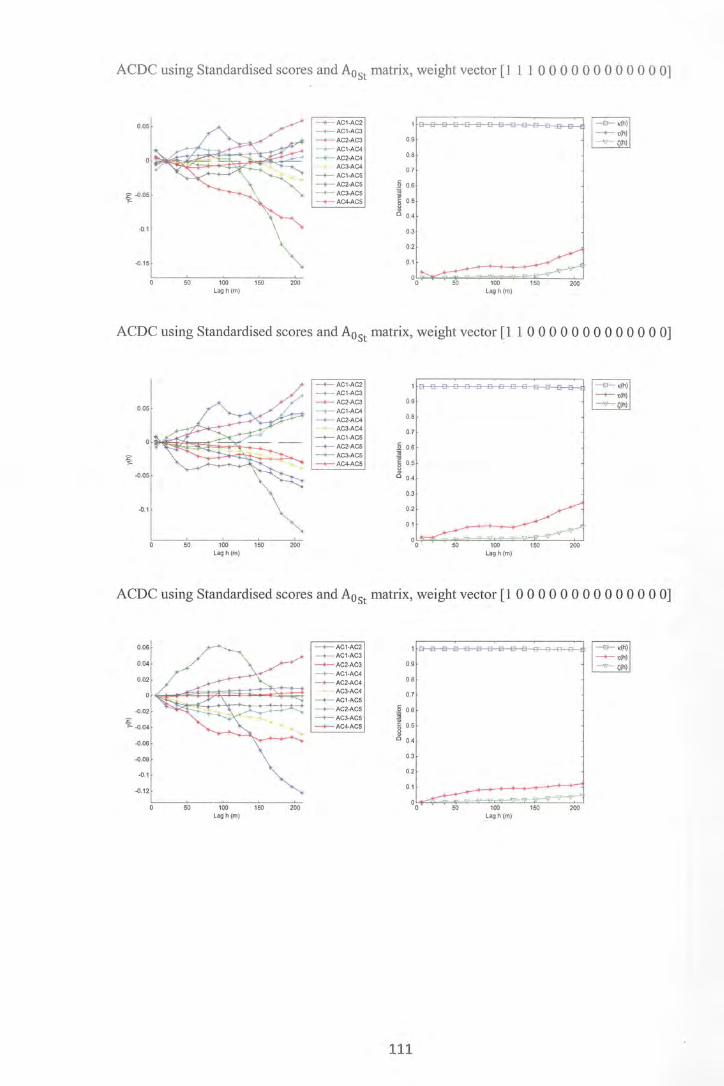
ACDC using Standardised scores and A05t matrix, weight vector [1 1 1 0 0 0 0 0 0 0 0 0 0 0 0]
--t- AC1 -AC2 --t- AC1-AC3 --t- AC2-AC3 0.9
-t-- AC1 -AC4
--t- AC2-AC4 0.8
AC3-AC4 0.7 -t- AC1-AC5
--t- AC2-AC5 .2 0.6 ---- AC3-AC5 ;;;
a; --+-- AC4-AC5 ~ 0.5
0 0.4
0.3
0.2
50 100 150 200 Lag h (m)
ACDC using Standardised scores and A05t matrix, weight vector [1 1 0 0 0 0 0 0 0 0 0 0 0 0 0]
--t- AC1-AC2 --t- AC1-AC3 --+-- AC2-AC3 0.9
-t-- AC1-AC4
--t- AC2-AC4 AC3-AC4
--t- AC1-AC5 --t- AC2-AC5 --+-- AC3-AC5 --+-- AC4-AC5
0.8
0.7
.Q 0.6 ;;; a;
~ 0.5
0 0.4
0.3
ACDC using Standardised scores and A05t matrix, weight vector [1 0 0 0 0 0 0 0 0 0 0 0 0 0 0]
--t- AC1-AC2 -+- AC1-AC3
--t- AC2-AC3 0.9
-4- AC1-AC4
--t- AC2-AC4 0.8
AC3-AC4 0.7 --t- AC1-AC5 --+-- AC2-AC5 0.6 -t-- AC3-AC5 --t- AC4-AC5 0.5
0.4
0.3
-0.1 0.2
-0.12 0.1
0 50 100 150 200 0
Lag h (m) Lag h (m)
111

Appendix 6- MATLAB CODES
6.1 ACDC code function [A,Lam,Nit,Cls]= ...
acdc(M,w,TOL,AO,LamO);
%acdc: appoximate joint diagonalization %(in the direct Least-Squares sense) of %a set of Hermitian matrices, using the %iterative AC-DC algorithm. 9,-0
%the basic call: %[A,Lam]=acdc(M); 9,-0
%Inputs: 9,-0
%M(N,N,K) - the input set of K NxN % "target matrices". Note that % all matrices must be % % 9,-0
9,-0
% % %
Hermitian (but need not be positive-definite) . If they are not Hermitian, an equivalent problem can always be formulated using Hermitian matrices.
%Outputs: % %A(N,N) - the diagonalizing matrix. % %Lam(N,K) - the diagonal values of the K % diagonal matrices. 9,-0
%The algorithm finds an NxN matrix A and %K diagonal matrices % L (: r :I k) =diag (Lam (:, k)) %such that % c_{LS}= % \sum_k\IM(:, :,k)-A*L(:, :,k)*A'\I_FA2 %is minimized. %
%-----------------------------------------% Optional additional input/output % parameters: %-----------------------------------------% %[A,Lam,Nit,Cls]= % acdc(M,w,AO,LamO); % %(additional) Inputs: 9,-0
%w(K) - a set of positive weights such that % C_{LS}= % \ s urn_ k \ w ( k) I M ( : , : , k) -A* L ( : , : , k) *A ' \ I_ FA 2 % Default: w=ones(K,l); 9-0
%AO - an initial guess for A % default: eye(N); %
112

%Lam0 - an initial guess for the values of % Lam. If specified, an AC phase is % run first; otherwise, a DC phase is % run first. S-o
%(additional) Outputs: So
%Nit - number of full iterations % %Cls - vector of Nit Cls values S-o
%-----------------------------~-----------% Additional fixed processing parameters %-----------------------------------------% %TOL -S-o
S-o
% % %
a tolerance value on the change of c_{Ls}. AC-DC stops when the decrease of C_{LS} is below tal. Originally set to:
10A-3/(N*N*sum(w));
%MAXIT - maximum number of allowed full S-o iterations. S-o Originally set to: 50; S-o
%INTLC - number of AC sweeps to interlace % de sweeps. % Originally set to: 1. % %-----------------------------------------% %Note that the implementation here is %somewhat wasteful (computationally) , %mainly in performing a full eigenvalue %decomposition at each AC iteration, %where in fact only the largest eigenvalue %(and associated eigenvector) are needed, %and could be extracted e.g. using the %power method. However, for small N (<10), %the matlab eig function runs faster than %the power method, so we stick to it.
%-----------------------------------------%version R1.0, June 2000. %By Arie Yeredor [email protected] S-o
%rev. R1.1, December 2001 %forced s=real(diag(S)) rather than just s=diag(S) %in the AC phase. S is always real anyway; however, %it may be set to a complex number with a zero %imaginary part, in which case the following %max operation yields the max abs value, rather %than the true max. This fixes that problem. -AY S-o
%Permission is granted to use and %distribute this code unaltered. You may %also alter it for your own needs, but you %may not distribute the altered code %without obtaining the author's explicit %consent. %comments, bug reports, questions %and suggestions are welcome. S-o
113

%References: %[1] Yeredor, A., Approximate Joint %Diagonalization Using Non-Orthogonal %Matrices, Proceedings of ICA2000, %pp.33-38, Helsinki, June 2000. %[2] Yeredor, A., Non-Orthogonal Joint %Diagonalization in the Least-Squares %Sense with Application in Blind Source %Separation, IEEE Trans. On Signal Processing, %vol. 50 no. 7 pp. 1545-1553, July 2002.
[N N1 K]=size(M); if N-=N1
error('input matrices must be square'); end if K<2
error('at least two input matrices are required'); end
if exist('w', 'var') & -isempty(w) W=W(:) i
if length(w)-=K error('length of w must equal K')
end if any(w<O)
error('all weights must be positive'); end
else w=ones(K,1);
end
if exist('AO', •var') & -isempty(AO) [NAO,Nc]=size(AO); if NAO-=N
error('AO must have the same number of rows as the target matrices')
else
end
end
AO=eye (N); Nc=N;
if exist('LamO', •var') & -isempty(LamO) [NLO,'KLO]=size(LamO); if NLO-=Nc
error('each vector in LamO must have M elements') end if KLO-=K
error('LamO must have K vectors') end if -isreal(LamO)
error('LamO must be real') end skipAC=O;
else skipAC=1;
end
%-----------------------------------------% here's where the fixed processing% parameters are set (and may be
114

% modified) : %-----------------------------------------%TOL=le-3/(N*N*sum(w)); %MAXIT=50; MAXIT=lOOOOO; %MAXIT=1000000; INTLC=l;
%-----------------------------------------and this is where we start working
%-----------------------------------------
Cls=zeros(MAXIT 1 1); Lam= zeros (N r K) ; A=AO; for Nit=l:MAXIT
if -skipAC
%AC phase for nsw=1:INTLC
for 1=1:Nc P=zeros (N) ; for k=l:K
D=M ( : I : I k) i
for nc=[l:l-1 1+1:Nc] a=A(: rnc); D=D-Lam(ncrk)*a*a';
end
end P=P+w(k)*Lam(l 1 k)*D;
[V S] =eig (P) ; s=real(diag(S)); [vix 1 mix]=max(s); if vix>O
%R1.1 - ay
al=V(: 1 mix); %this makes sure the 1st nonzero %element is positive 1 to avoid %hopping between sign changes: fnz=find(al-=0); al=al*sign(al(fnz(l))); lam=Lam (lr :) ; f=vix/((lam.*lam)*w}; a=al*sqrt(f);
else a=zeros(Nr1);
end A (: r 1) =a;
end %sweep end %interlaces
end %skip AC skipAC=O;
%DC phase AtA=A' *A; AtA2=AtA.*conj (AtA); G=inv(AtA2); for k=1:K
Lam(: /k) =G*diag(A' *M(: I: rk) *A) i
L=diag(Lam(: 1 k)); D=M(: I: /k) -A*L*A' i
Cls(Nit)=Cls(Nit)+w(k)*sum(sum(D.*conj (D)));
115
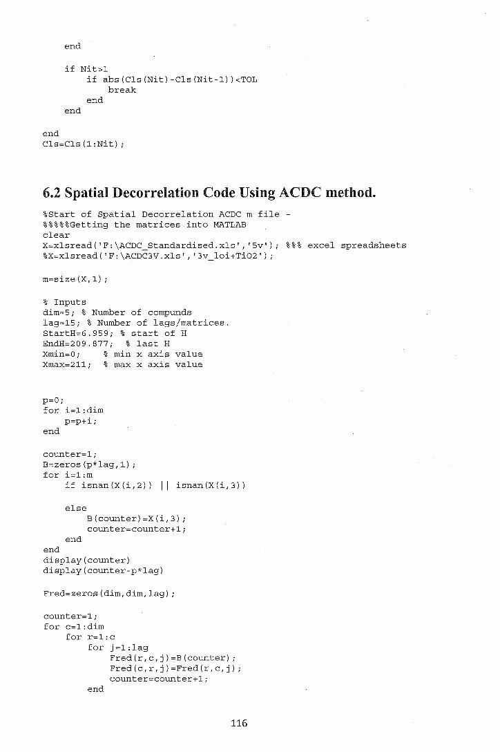
end
if Nit>l if abs(Cls(Nit)-Cls(Nit-l))<TOL
break end
end
end Cls=Cls(l:Nit);
6.2 Spatial Decorrelation Code Using ACDC method. %Start of Spatial Decorrelation ACDC m file -%%%%%Getting the matrices into MATLAB clear X=xlsread('F:\ACDC_Standardised.xls', '5v'); %%%excel spreadsheets %X=xlsread('F:\ACDC3V.xls', '3v_loi+Ti02');
m=size(X,l);
% Inputs dim=5; % Number of compunds lag=15; % Number of lags/matrices. StartH=6.959; % start of H EndH=209.877; % last H Xmin=O; % min x axis value Xmax=211; % max x axis value
p=O; for i=l:dim
p=p+i; end
counter=l; B=zeros(p*lag,l); for i=l:m
if isnan(X(i,2)) II isnan(X(i,3))
end
else B(counter)=X(i,3); counter=counter+l;
end
display(counter) display(counter-p*lag)
Fred=zeros(dim,dim,lag);
counter=l; for c=l:dim
for r=l:c for j=l:lag
Fred(r,c,j)=B(counter); Fred(c,r,j)=Fred(r,c,j); counter=counter+l;
end
116

end end
display(counter-1) M=Fred
%Getting the off diagonal values from the expeimental semivariogram matrices m=zeros(O.S*dim*(dim+1) ,lag); figure counter=1; for counter1=1:dim
end
for counter2=1:counter1
end
for i=1:lag m(counter,i)=M(counter2,counter1,i);
end counter=counter+1;
%%%%%%%%%%%%%%%%%%Experimental Cross semivariograms counter=1; mr=zeros(O.S*dim*(dim-1),lag); % mr=off diagonal values of exp semivariogram
· md=zeros (dim, lag); % md=diagonal values of exp. semivariograms for i=1:0.5*dim*(dim+1)
end
if i==0.5*counter*(counter+1) md(counter, :)=m(i, :) ; counter=counter+1;
else mr(i+1-counter, :)=m(i, :) ;
end
hold on l=linspace(StartH,EndH,lag); z=zeros(lag,1); plot (l,mr, '-*') plot(l,z, 'k--') xlabel ('Lag h (m) ') ylabel ('\gamma (h) ' ) hold off Ymin=(min(min(mr)))*1.1; Ymax=(max(max(mr)))*1.1; axis ( [Xmin Xmax Ymin Ymax])
%%%%%%%%%%%Legends for variables legendS= legend('Fe & Al_20_3', 'Si0_2 & Al_20_3'i 'SiO 2 & Fe', 'TiO 2 & Al_20_3', 'Ti0_2 & Fe', 'Ti0_2 & Si0_2', 'Al_20_3 & LOI', 'LOI & Fe', 'LOI & Si0_2', 'LOI & Ti0_2', 'Location', 'NEO');
%%%%%%%%Titles h=Title('Cross Semivariograms of Standardised Variables') %h=Title('Cross Semivariograms of Normal Score Variables') set(h, 'FontSize',12, 'FontWeight', 'bold');
%%%%%%%%%%%%% ACDC Algorithms
A0=[0.505 0.1385 -0.3394 -0.6989 -0.3494; matrix using standardised data
-0.5197 0.1936 -0.2077 0.1586 0.4069 -0.5783 0.467 0.1988 0.4688 0.0715 -0.5987 0.6455
-0.79; -0.4923; -0.0038;
117
%PCA eigenvectors

0.2992 0.777 0.5149 0.1736 -0.1069];
%AO= [ 0.4995 -0.2914 -0.3244 0.7085 0.2416 %PCA eigenvector matrix using normal scores data % -0.5131 -0.3250 -0.1737 -0.1130 0.7670 % 0.3927 0.6743 0.2085 -0.1020 0.5807 ;
% 0.4789 -0.2269 -0.5185 -0.6711 0.0079; % 0.3220 -0.5507 0.7432 -0.1566 0.1273 l ;
w=[1,0,0,0,0,0,0,0,0,0,0,0,0,0,0]; %%%weigh vector NitTemp=1; TOL=1e-16;
[A,D,Nit,Cls]=acdc(M,w,TOL); %%%%%%%%%% ACDC with no AO [A,D,Nit,Cls]=acdc(M,w,TOL,AO); %%%%%%%%%%ACDC with an AO
%%%%%%%%%%%End of ACDC
inv(A) %%%% transformation matrix
display(M) % matrices of experimental semivariogram matrices b3=zeros(dim,dim,lag); for i=1:lag
b3(:, :,i)=inv(A)*M(:, :,i)*inv(A 1); %%Obtaining the Factor
matrices end display(b3) % decorrelated factor matrices
%%%%%%Getting the cross validation decorrelated Factor values from the matrices into vectors for plotting )
b=zeros(0.5*dim*(dim+1) ,lag);
counter=1; for counter1=1:dim
for counter2=1:counter1 for i=1:lag
b(counter,i)=b3(counter2,counter1,i);
end end
end counter=counter+1;
figure counter=1; br=zeros(0.5*dim*(dim-1) ,lag); bd=zeros(dim,lag); for i=1:0.5*dim*(dim+1)
end
if i==0.5*counter*(counter+1) bd(counter, :)=b(i, :) ; counter=counter+1;
else br(i+1-counter, :)=b(i, :) ;
end
hold on l=linspace(StartH,EndH,lag); z=zeros(lag,1); plot ( 1, br I I *- I )
plot(l,z, 1 k-- 1 )
xlabel ( 1 Lag h (m) 1 )
ylabel ( 1 \gamma (h) 1 )
% br=off diagonal factor values % bd=diagonal factor values
118

hold off Ymin=(min(min(br)))*1.1; Ymax=(max(max(br)))*1.1; axis([Xmin Xmax Ymin Ymax]) legendS= legend('AC1-AC2' 1 'AC1-AC3' 1 'AC2-AC3' 1 'AC1-AC4' 1 'AC2-AC4'1 'AC3-AC4' I 'AC1-AC5'/ 'AC2-AC5'/ 'AC3-AC5' I 'AC4-AC5' 1 'Location' 1 'NEO'); br;
% Zeta values and plot yy=(br) ."2; zeta=sum(yy)*2 figure l=linspace(StartH 1EndH 1lag) ;%****???? z=zeros(lag 11); plot(l 1zeta 1 'g-v' 1 1 1 Z 1 'k--') xlabel ('Lag h (m) ' ) ylabel('\zeta(h) ') z1=min(zeta) z2=max (zeta); Ymin=z1-(z1*0.1); Ymax=z2+(z2*0.1); axis([Xmin Xmax Ymin Ymax]) legend('\zeta(h) 1
1 'Location'/ 'NEO');
% Average Zeta Value Avezeta=sum(zeta)/lag
%Tau Values and plot xx= sum(abs(br))*2; rr=sum (abs (bd)) ; tau= (xx) . I (rr) figure l=linspace(StartH 1EndH 1lag) ;%****???? z=zeros(lag 11); plot (1 1 tau/' r-*' 1 1 1 Z 1 'k--') xlabel ('Lag h (m) ') ylabel ( ' \tau (h) ' ) z1=min (tau); z2=max (tau); Ymin=z1-(z1*0.1); Ymax=z2+(z2*0.1); axis ( [Xmin Xmax Ymin Ymax]) legend('\tau(h) ' 1 'Location' 1 'NEO');
%Average Tau AveTau=sum(tau)/lag
% Kappa Value and plot ·jj=(mr) ."2; ori=sum(jj)*2; ii=zeta./ori; kappa=1-ii figure l=linspace(StartH1EndH 1lag); z=zeros(lag 11); plot(l 1kappa 1 'b-S 1 1l 1Z 1 'k--') xlabel ('Lag h (m) ') ylabel ( ' \kappa (h) ' )
z1=min(kappa); % very high negative values z2=max (kappa); Ymin=z1+(z1*0.1);
119

Ymax=z2-(z2*0.1); zl=min(kappa); % positive z2=max (kappa) ; Ymin=zl-(zl*O.l); %Ymin=O; Ymax=z2+(z2*0.1); axis([Xmin Xmax Ymin Ymax]) legend('\kappa(h) ','Location', 'NEO');
%Average Kappa AveKappa=sum(kappa)/lag
%Plot for all spatial decorrelation measures figure linspace(StartH,EndH,lag); z=zeros(lag,l); plot(l,kappa, 'b-s' ,l,tau, •r-*' ,l,zeta, 'g-v' ,l,z, 'k--') xlabel ('Lag h (m) • ) ylabel('Decorrelation') Ymin=[]; Ymax=[];
% zl=min(kappa); % Very negative values % z2=max(zeta); % Ymin=zl+(zl*O.l); % Ymax=z2+(z2*0.1);
Ymin=O; Ymax=l.OS; axis([Xmin Xmax Ymin Ymax]) %% Create legend legendl = legend('\kappa(h) ', '\tau(h) ', '\zeta(h) ','Location', 'NEO'); %%%%%%%%%%%%%Titles
%h=Title('ACDC using Normal scores and AO_N_S') %h=Title('ACDC using Normal scores') h=Title('ACDC using Standardised scores and AO_S') %h=Title('ACDC using Standardised scores') set(h, 'FontSize' ,12, 'FontWeight', 'bold');
%%%%%%%% Eigenvalues of Experimental semivariogram matrices for i=l:lag
eig (M ( : , : , i) ) end
%%%%%%%%%%Average Spatial Decorrelation Measures Avezeta AveTau AveKappa
%%%%%%%%%%%Plot the direct semivariograms m=zeros(O.S*dim*(dim+l) ,lag); figure counter=l; for counterl=l:dim
for counter2=l:counterl for i=l:lag
m(counter,i)=M(counter2,counterl,i);
end end
end counter=counter+l;
counter=l;
120

mr=zeros(0.5*dim*(dim-1) ,lag); % mr=off diagonal values of exp semivariogram md=zeros(dim,lag); % md=diagonal values of exp. semivariograms for i=1:0.5*dim*(dim+l)
end
if i==0.5*counter*(counter+l) md(counter, :)=m(i, :) ; counter=counter+l;
else mr (i+l-counter, :) =m (i, :) ;
end
hold on l=linspace(StartH,EndH,lag) ;%****???? z=zeros(lag,l); plot (l,md, '-*') plot (l, z, 'k-- ') xlabel ('Lag h (m) ' ) ylabel ('\gamma (h) ' ) hold off Ymin=(min(min(md))); Ymax=(max(max(md)))*l.l; axis([Xmin Xmax Ymin Ymax])
%Legends legendS = legend('Al 20_3', 'Fe', 'Si0_2', 'Ti0_2', 'LOI', 'Location', 'NEO'); %h=Title('Experimental Direct Semivariograms of Standardised
Variables ' ) h=Title('Experimental Direct Semivariograms of Normal Score Variables' ) set(h, 'FontSize' ,12, 'FontWeight', •bold');
6.3 Spatial Decorrelation Code Using MAF and PCA Factors %M-File used to obtain MAF and PCA spatial decorrelation results clear; A=xlsread('F:\MAF&PCA_5V.xls', 'MAF5_S'); stats
m=size(A,l);
% Inputs dim=5; % Number of compunds lag=15; % Number of lags/matrices. StartH=6.959; %start of H EndH=209.877; % last H Xmin=O; % min x axis value Xmax=210; % max x axis value
p=O; for i=l:dim
p=p+i; end
counter=l; B=zeros(p*lag,l);
121
% The MAF/PCA factor global

for i=1:m if isnan(A(i,2)) II isnan(A(i,3))
else
end end
B(counter)=A(i,3) i
counter=counter+1i
display(counter) display(counter-p*lag)
Fred=zeros(dim,dim,lag) i
counter=1i for c=1:dim
for r=1:c for j=1:lag
Fred(r,c,j)=B(counter) i
Fred(c,r,j)=Fred(r,c,j) i
counter=counter+1i end
end end
display(counter-1)
b3=Fred display(b3) % decorrelated matrices
%Getting the cross validation decorrelated values from the matrices into %vectors for plotting
b=zeros(0.5*dim*(dim+1) ,lag) i
counter=1i for counter1=1:dim
for counter2=1:counter1 for i=1:lag
b(counter,i)=b3(counter2,counter1,i) i
end end
figure
end counter=counter+1i
counter=1i br=zeros(O.S*dim*(dim-1) ,lag) i % br=off diagonal values bd=zeros(dim,lag) i % bd=diagonal values for i=1:0.5*dim*(dim+1)
end
if i==0.5*counter*(counter+1) bd(counter, :)=b(i, :) i
counter=counter+1i else
br (i+1-counter, :) =b (i, :) i
end
hold on l=linspace(StartH,EndH,lag) i
z=zeros(lag,1) i
122
plot (l,br, '*-') plot(l,z, 'k--') xlabel ('Lag h (m) ' ) ylabel ('\gamma (h) ' ) hold off %end of boogie Ymin=-0.1S Ymax=0.1S %Ymin=(min(min(br)))*1.1; %Ymax=(max(max(br)))*1.1; axis([Xmin Xmax Ymin Ymax] )% might need to change (,, min value of b and maximum value of b)
%LEGENDS
legendS= legend('M1-M2'r 'M1-M3'r 'M2-M3', 'M1-M4', 'M2-M4', 'M3-M4 1 , 'M1-MS'r 'M2-MS' 1 'M3-MS'r 'M4-MS', 'Location'r 'NEO'); %legendS= legend('PC1-PC2', 'PC1-PC3', 'PC2-PC3', 'PC1-PC4 1 , 'PC2-PC4', 'PC3-PC4', 'PC1-PCS', 'PC2-PCS', 'PC3-PCS', 'PC4-PCS'r 'Location'r 'NEO'); %h=Title('Cross Semivariograms of MAF Factors using Normal Scores'); h=Title('Cross Semivariograms of MAF Factors using Standardised Scores') set(h 1 'FontSize',12, 'FontWeight', 'bold'); br % zeta yy=(br) .A2; zeta=sum(yy)*2 figure l=linspace(StartH,EndH,lag) ;%****???? z=zeros(lag 1 1); plot(l 1 zeta, 'g-v',l,z, 'k-- 1 )
xlabel ( 'Lag h (m) ' ) ylabel ( '\gamma (h) ' ) %z1=min (zeta); z2=max(zeta); Ymin=O; %Ymin=z1-(z1*0.1); Ymax=z2+(z2*0.2); axis ( [Xmin Xmax Ymin Ymax] ) legend('\zeta(h) ','Location', 'NEO');
% Average Zeta AveZeta=sum(zeta)/lag
%tau xx= sum(abs(br))*2; rr=sum(abs(bd)); tau=(xx) ./(rr) figure l=linspace(StartH,EndH,lag) ;%****???? z=zeros(lag 1 1); plot(l,tau 1 'r-*' ,l,z, 'k-- 1 )
xlabel ('Lag h (m) ') ylabel ( '\gamma (h) 1 )
%z1=min (tau) ; z2=max (tau); %Ymin=z1-(z1*0.1); Ymin=O; Ymax=z2+(z2*0.1); axis([Xmin Xmax Ymin Ymax]) legend('\tau(h) ','Location', 'NEO');
123

%Average Tau AveTau=sum(tau)/lag
%Get the experimental semivariogram Al=xlsread('F:\ACDC_Standardised.xls', 'Sv'); %Original experimental semivariogram results %Al=xlsread('F:\ACDC3V.xls', '3v_loi+Ti02');
m=size(Al,l);
% Inputs dim=5; % Number of compunds lag=15; %Number of lags/matrices. StartH=6.959; .% start of H EndH=209.877; % last H Xmin=O; % min x axis value Xmax=210; % max x axis value
p=O; for i=l:dim
p=p+i; end
counter=l; B=zeros(p*lag,l); for i=l:m
if isnan(Al(i,2)) II isnan(Al(i,3))
end
else B(counter)=Al(i,3); counter=counter+l;
end
display(counter) display(counter-p*lag)
counter=l; for c=l:dim
for r=l:c for j=l:lag
Fredl(r,c,j)=B(counter); Fredl(c,r,j)=Fredl(r,c,j); counter=counter+l;
end end
end
display(counter-1) M=Fredl
%kappa
% Start of getting the off diagonal values from the origianl experimental % semivariograms matrices
124

m=zeros(O.S*dim*(dim+l) ,lag);
counter=l; for counterl=l:dim
for counter2=1:counterl for i=l:lag
m(counter,i)=M(counter2,counterl,i);
end end
end counter=counter+l;
counter=l; mr=zeros(O.S*dim*(dim-l),lag); % mr=off diagonal values of exp semivariogram md=zeros(dim,lag); % md=diagonal values of exp. semivariograms for i=l:O.S*dim*(dim+l)
end
if i==0.5*counter*(counter+l) md(counter, :)=m(i, :) ; counter=counter+l;
else mr(i+l-counter, :)=m(i, :) ;
end
%end of getting values and start of kappa
j j = ( mr) . "'2 ; ori=sum(jj)*2; ii=zeta./ori; kappa=l-ii figure l=linspace(StartH,EndH,lag) ;%****???? z=zeros(lag,l); plot(l,kappa, 'b-s',l,z, 'k--') xlabel ('Lag h (m) ' ) ylabel ( '\gamma (h) ' ) %zl=min(kappa) z2=max (kappa) ; %Ymin=Zl-(zl*O.Ol) Ymin=O; Ymax=z2+(z2*0.1); axis([Xmin Xmax Ymin Ymax]) legend('\kappa(h) ','Location', 'NEO');
%Average Kappa AveKappa=sum(kappa)/lag
%plot all averages figure linspace(StartH,EndH,lag); z=zeros(lag,l); plOt ( l, kappa I I b- S I I 1, taU I I r- * I 1 l, Zeta 1 I g -V I I 1, Z 1 I k- - I )
xlabel ('Lag h (m) ' ) ylabel('Decorrelation') Ymin=[]; Ymax=[]; zl=min(zeta); Ymin=zl-(zl*O.S); Ymax=max(kappa)*l.l; axis( [Xmin Xmax Ymin Ymax])
125

%% Create legend legendl = legend('\kappa(h) ', '\tau(h) ', '\zeta(h) ','Location', 'NEO'); %h=Title('MAF using Normal scores') h=Title('MAF using Standardised scores') set(h, 'FontS~ze' ,12, 'FontWeight', 'bold'); for i=l:l5
eig (M ( : , : , i) ) end
AveZeta A veT au AveKappa
126


![[188]Comparison of Fuzzy Reasoning Methods](https://img.dokumen.tips/doc/110x75/55cf854a550346484b8c6328/188comparison-of-fuzzy-reasoning-methods.jpg)