Comparing vector–host and SIR models for dengue

transmission

Abhishek Pandeya,∗, Anuj Mubayib, Jan Medlockc

aDepartment of Mathematical Sciences, Clemson University, Clemson, South Carolina 29634,USA

bDepartment of Mathematics, Northeastern Illinois University, Chicago, Illinois 60625, USAcDepartment of Biomedical Sciences, Oregon State University, Corvallis, Oregon 97331, USA

Abstract

Various simple mathematical models have been used to investigate dengue transmis-sion. Some of these models explicitly model the mosquito population, while othersmodel the mosquitoes implicitly in the transmission term. We study the impactof modeling assumptions on the dynamics of dengue in Thailand by fitting denguehemorrhagic fever (DHF) data to simple vector–host and SIR models using BayesianMarkov chain Monte Carlo estimation. The parameter estimates obtained for bothmodels were consistent with previous studies. Most importantly, model selectionfound that the SIR model was substantially better than the vector–host model forthe DHF data from Thailand. Therefore, explicitly incorporating the mosquito pop-ulation may not be necessary in modeling dengue transmission for some populations.

Keywords: Dengue, mathematical model, parameter estimation, Markov chainMonte Carlo (MCMC)

1. Introduction

Dengue infection is one of the leading causes of illness in the tropics and subtrop-ics, where it inflicts substantial health, economic and social burdens [1]. Humansare infected with dengue viruses by the bite of an infective female mosquito Aedesaegypti, the principal vector of dengue. Once a person gets bitten by an infectivemosquito, the virus undergoes an incubation period of about 4 to 7 days, after which

∗Corresponding author:Abhishek Pandey,O-110 Martin Hall, Box 340975,Clemson, SC 29634-0975, USA;Email: abhishe@g.clemson.edu; Phone: +1 (864) 633 9240

Preprint submitted to Mathematical Biosciences October 9, 2013

the person enters the acute phase of infection. The acute phase can be as short as 2days and as long as 10 days. If other female A. aegypti mosquitoes bite the ill personduring this acute phase, those mosquitoes may become infected and subsequentlybegin the transmission cycle anew. Dengue infection is generally characterized by asudden onset of fever and other nonspecific signs and symptoms, including frontalheadache, body aches, nausea and vomiting [2]. Symptoms range from mild fever tohigh fever with severe headache and joint pain, and even to internal hemorrhaging,circulatory failure and death. Cases are classified, in order of increasing severityas dengue fever, dengue hemorrahagic fever (DHF) and dengue shock syndrome [3].Dengue has been recognized in over 100 countries and an estimated 50–100 millioncases of dengue fever and several hundred thousand DHF cases occur yearly, depend-ing on epidemic activity [4]. Particularly, in Thailand, dengue disease incidence hasincreased from 9 per 100 000 in 1958 to 189 per 100 000 in 1998, with the largestreported incidence of 325 per 100 000 in 1987, making dengue a severe public healthproblem in Thailand [5].

Several mathematical models have been proposed to investigate dengue epidemi-ology, some of which explicitly model the mosquito population [e.g. 3, 6, 7], whileothers implicitly model it in the transmission term [e.g. 8–10]. Although both kindsof models have been extensively used for dengue, little guidance exists for which typeof model should be preferred. In particular, there has been no comparison of howwell these models explain observed incidence. In this study, we considered simpledengue models with and without explicitly modeling mosquitoes, fit both models toDHF incidence data, and used model selection to compare the models.

Fitting models to data validates the model as well as provides estimates of un-known model parameters. There are some examples in the literature where denguemodels have been fit to data. Chowell et al. [11] estimated the transmissibility ofdengue during a 2002 epidemic in the Mexican state of Colima using municipal epi-demic data to evaluate the effect of spatial heterogeneity. Ferguson et al. [12] usedlongitudinal incidence of serious dengue disease from Thailand and estimated thebasic reproductive number R0 to gain insight into the transmission dynamics andepidemiology of dengue. We fit a simple vector–host dengue model as well as anSIR-type dengue model and obtain estimates of unknown parameters like recoveryrate, probability of severe form of disease, mosquito mortality rate, etc.

The goal of the present study is to understand the impact of some modelingassumptions on quantifying estimates of epidemiological metrics for dengue. We ap-plied Bayesian Markov chain Monte Carlo (MCMC) estimation on a simple vector–host dengue model as well as an SIR-type dengue model to estimate model parame-ters using monthly DHF incidence data in Thailand for January 1984 to March 1985.

2

The Bayesian MCMC techniques that we used in this study have been commonlyused to estimate model parameters of infectious diseases [13–16]. We use the poste-rior distribution of the model parameters obtained from Bayesian MCMC to performuncertainty and sensitivity analysis of basic reproductive number R0 and thereafter,use model selection on a set of vector–host and SIR models to find a model whichagrees with the data most parsimoniously.

2. Methods

We built two mathematical models of dengue transmission, one in which themosquitoes are explicitly tracked and another without explicit mosquito populations.We then used Bayesian MCMC to fit DHF data from Thailand to these two models.In this section, we outline the data source, models and methods and refer to moredetailed descriptions in the Supplementary Material.

2.1. Data Source

The Thailand Ministry of Public Health have been recording the number of DHFcases since 1972. Cases are diagnosed using criteria established by the World HealthOrganization. We obtained the monthly incidence of DHF for Thailand from 1983to 1997 (Figure 1) [17]. We chose one epidemic, from January 1984 to March 1985(Figure 2), to fit the dengue models: this particular epidemic was chosen as a clear,representative example among this data. More specifically, we used the cumulativemonthly number of DHF cases for the period January 1984 to March 1985. Cumula-tive incidence is generally smoother than the original incidence data and thus easierto fit and it also easily handles delayed reporting on holidays and weekends.

2.2. Vector–host model

The Ross–Macdonald model, originally developed for malaria, is a standard math-ematical model for vector-borne pathogens that tracks infections in both humans andmosquitoes [18]. Following this framework, we built a vector–host model for dengueconsisting of three human host compartments, susceptible (the number of susceptiblehumans isHS), infectious (HI) and recovered (HR), and two mosquito compartments,susceptible (VS) and infectious (VI). Mosquitoes do not recover from infection. The

3

model is the system of differential equations

dHS

dt= BH −mcβH

VIVHS − µHHS,

dHI

dt= mcβH

VIVHS − γHHI − µHHI ,

dHR

dt= γHHI − µHHR,

dVSdt

= BV − cβVHI

HVS − µV VS,

dVIdt

= cβVHI

HVS − µV VI ,

(1)

where H = HS +HI +HR and V = VS +VI are the human and mosquito populationsizes, respectively. A susceptible human gets infected with force of infection mcβH

VI

V,

where m is number of mosquitoes per person, c is mean rate of bites per mosquitoand βH is the mosquito-to-human transmission probability per bite. Infectious peo-ple recover at rate γH . The force of infection for mosquitoes is cβV

HI

H, where βV is

the human-to-mosquito transmission probability. For simplicity, we ignored disease-induced mortality in both humans and mosquitoes, which is small [19]. Because weonly fit the model to an epidemic lasting about a year, we assumed the human pop-ulation was constant size by using the birth rate BH = µHH. We also assumed themosquito population was constant size (BV = µV V ), neglecting seasonal fluctuationsfor simplicity.

Standard mathematical analysis of the model (Supplementary Material S1) showsthat the basic reproductive number, the number of new human infections caused bya single infected human in an otherwise completely susceptible population, is

R0 =mc2βHβV

µV (µH + γH). (2)

In addition, there are two equilibrium points, the disease-free equilibrium and theendemic equilibrium. An equilibrium point is asymptotically stable if nearby orbitsconverge to it as time increases, and it is globally asymptotically stable if all orbits,not just those nearby, converge to the equilibrium [20]. For R0 > 1, the disease-freeequilibrium is unstable and the endemic equilibrium is locally asymptotically stable.The disease-free equilibrium is globally asymptotically stable when R0 ≤ 1 (and theendemic equilibrium is out of the relevant state space, having HI and VI negative,and unstable).

To simplify the parameter estimation, rather than fitting human mortality ratealong with the other parameters, we fixed µH = 1/69 y−1 based on the average

4

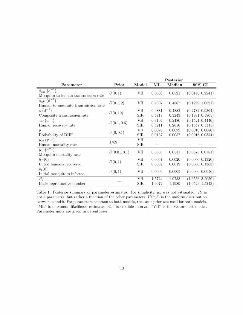
human duration of life in Thailand in 1984 of about 69 years [21]. The remain-ing unknown parameters are the human recovery rate (γH), the mosquito mortalityrate (µV ), the probability of DHF (p), the mosquito biting rate (c), the numberof mosquitoes per person (m), the mosquito-to-human transmission probability (βH)and the human-to-mosquito transmission probability (βV ). The biting rate, c, alwaysappears in the model multiplied with either βH or βV . Similarly, m always appearsmultiplied with βH . Therefore, only 2 of these 4 parameters can be separately esti-mated, which we chose to be βaH = mcβH and βaV = cβV . In addition, the initialproportion of humans recovered in the host population (hR(0) = HR(0)/H) as well asinitial proportion of mosquitoes infected in the vector population (vI(0) = VI(0)/V )are unknown and must be determined. Thus, we estimated a total of 5 unknownparameters and 2 initial conditions for the vector–host model. We used the inci-dence data for January 1984 and Thailand’s population in year 1984 to calculateinitial conditions for initial proportion of hosts infected, i.e. hI(0) = HI(0)/H(0),where HI(0) = 454 and H(0) = 46 806 000. Since both the human and mosquitopopulations are constant, initial proportions of susceptible humans and mosquitoeswere calculated using the other initial conditions, i.e. hS(0) = 1− hI(0)− hR(0) andvS(0) = 1− vI(0).

2.3. SIR model

Dengue transmission has been extensively modeled using SIR-type models, whichonly explicitly track human infections [e.g. 8–10]. These SIR models are simpler thanvector–host models, making analysis and parameter estimation easier. SIR modelsfor dengue have typically been constructed directly [e.g. 8]. Alternately, an SIR modelcan be derived from a vector–host model by assuming that infection dynamics in thevector are fast compared to those of the host, a quasi-equilibrium approximation[22].

We used a standard SIR model,

dHS

dt= BH − β

HI

HHS − µHHS,

dHI

dt= β

HI

HHS − γHHI − µHHI ,

dHR

dt= γHHI − µHHR,

(3)

where H = HS + HI + HR is the human population size. Again, we kept thepopulation size constant by setting the birth rate to BH = µHH. A susceptibleperson gets infected with force of infection βHI

H, where β is the composite human-

to-human transmission rate. Comparing the equilibria of the vector–host model and

5

the SIR model (Supplementary Material S2) provides β in terms of the parametersof the vector–host model:

β ≈ mc2βHβVµV

. (4)

SIR model (3) is a standard mathematical model for directly transmitted pathogenslike influenza and has been thoroughly analyzed [e.g. 23]. The basic reproductivenumber is

R0 =β

µH + γH. (5)

As with vector–host model (1), there are two equilibrium points, the disease-freeequilibrium and the endemic equilibrium: for R0 > 1 the disease-free equilibrium isunstable and the endemic equilibrium is globally stable, while the disease-free equi-librium is globally asymptotically stable for R0 ≤ 1 (with the endemic equilibriumhaving HI < 0 and being unstable).

The unknown parameters are the transmission rate (β), the recovery rate (γH) andthe probability of DHF (p), along with the initial proportion of humans recovered(hR(0) = HR(0)/H). As in the vector–host model, we used the fixed value forthe human mortality rate µH = 1/69 y−1 to simplify the parameter estimation.Again, the initial proportion of infected humans is given by hI(0) = HI(0)/H(0)with HI(0) = 454 and H(0) = 46 808 000. Like the vector–host model, the otherinitial condition is hS(0) = 1− hI(0)− hR(0).

2.4. Bayesian Markov chain Monte Carlo estimation

To estimate the unknown parameters, we used a Bayesian MCMC technique.Bayesian inference uses prior information of the model parameters from previousstudies, which is then combined with new data to generate estimates in the form of aprobability distribution for the parameters. More precisely, for parameters θ and dataD, with the prior parameter distribution Pr(θ) and likelihood function Pr(D | θ),the posterior parameter distribution Pr(θ | D) is given by Bayes’s Theorem:

Pr(θ | D) =Pr(D | θ) Pr(θ)

Pr(D)(6)

or, alternately,Pr(θ | D) ∝ Pr(D | θ) Pr(θ). (7)

Because there are no general closed-form solutions, MCMC or other methods mustbe used to generate approximate samples from the posterior parameter distributionPr(θ | D).

6

The connection between the data and the parameters is made by the likelihoodfunction L(θ) = Pr(D | θ), which is the conditional probability of obtaining the data(D) for the given parameter values (θ). Therefore, L(θ) needs to be maximized toobtain best-fit parameter set. In our case, the likelihood function is derived fromthe vector–host and SIR models, the solutions to which provide estimates of theDHF monthly incidence data. We added a compartment to each model to calculatethe cumulative number of DHF infections (HC). We assumed that a fraction p ofinfections were diagnosed as DHF, with p constant in time. We added differentialequations for the HC compartment,

dHC

dt= pmcβH

VIVHS, (8)

for the vector–host model, and

dHC

dt= pβ

HI

HHS, (9)

for the SIR model, which are precisely the rates of new infections multiplied by p.The “ode15s” function in Matlab was used to numerically solve the vector-host model(1) & (8) and the SIR model (3) & (9). These numerical solutions give the predictedmonthly cumulative DHF incidence, yi = HC(ti)/H, where ti = 0, 30, 60, ... days.Using the least-squares error between the cumulative DHF data Di and the modelprediction,

E2 =15∑i=1

(Di − yi(θ)

)2, (10)

we assumed the errors were Gaussian, giving the likelihood function

L(θ) = Pr(D | θ) = exp(−E2

). (11)

For the prior parameter distributions, we assigned wide uniform distributions,with ranges chosen to represent our general understanding about where the param-eter values may lie. In the absence of any information on parameters estimates, weused least-squares fitting to find best-guess estimates of parameters. Estimates of γH ,µV and µH from the literature (γH = 1/7 d−1, µV = 1/14 d−1 and µH = 1/69 y−1)were used and the vector–host model was fitted to the data using least squaresin Berkeley Madonna to find initial point estimates βaH = 0.002, βaV = 1.8 andp = 0.04. We used these initial point estimates to form uniform priors for theseparameters such that their point estimates lie inside the range of priors. For thetransmission term β of the SIR model, we simply choose a very wide uniform prior.

7

Where parameters were common to both models, both models used the same prior(Table 1).

To generate the posterior parameter distribution, we used an MCMC methodbased on the Metropolis algorithm using a Gaussian jumping distribution with anadaptive covariance matrix. For each model, we simulated 4 independent MCMCchains and used the Gelman–Rubin test to determine when the chains had convergedto the stationary distribution, i.e. the parameter posterior distribution. The Gelman–Rubin test signals convergence when the variance between independent chains issimilar to the variance within the chains. (See Supplementary Material S3 for moredetails.) Once the Gelman–Rubin test passed, we continued sampling from one ofthe chains for 10 000 more iterations without updating the covariance matrix, savingevery 5th iterate as the posterior parameter distribution.

3. Results

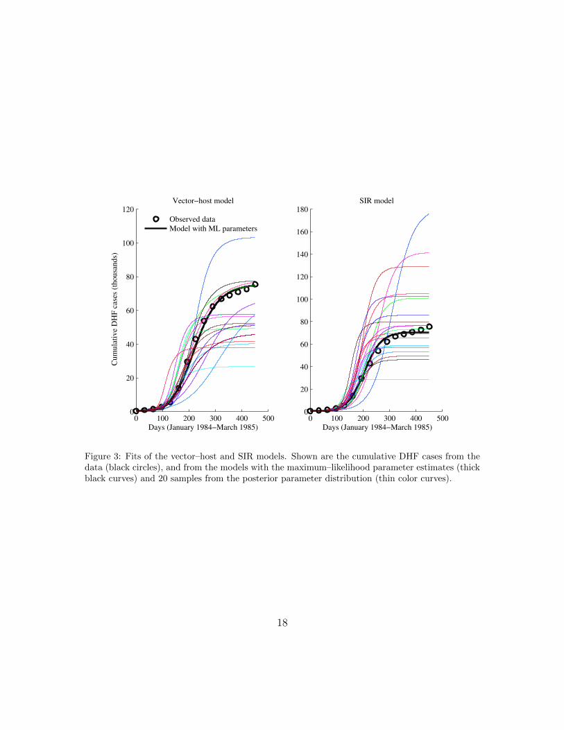
We estimated 7 total parameters for the vector–host model and 4 total parametersfor the SIR model by Bayesian MCMC using the cumulative DHF incidence data.Both models with their maximum-likelihood (ML) parameter estimates fit the datawell (Figure 3), with the vector–host model fitting slightly better. (More on modelfitting and model selection below.)

The estimates of the human recovery rate were similar for both models (Fig-ure 4(d) and Table 1). The average duration of human dengue infection is between2 and 7 days approximately, with ML estimates of about 2 to 3 days. The initialproportion of humans recovered (hR(0)) was estimated to be small in both models,indicating that the human populations were almost entirely susceptible when theoutbreak started.

Estimates of the probability of DHF differed somewhat between models: ML ofaround 3 DHF cases per 1000 infections from the vector–host model and around 14DHF cases per 1000 infections from the SIR model. The vector–host model includesseveral parameters not present in the SIR model. From the vector–host model, therange of average lifespan of mosquitoes (1/µV ) was found to be approximately 13 to26 days, with ML estimate of about 15 days. The initial proportion of mosquitoesinfected was very small (ML of about 0.5%), so that the outbreak had just startedin the mosquitoes as well as the humans.

The transmission rates are not common between the models, but comparison ofequilibria of both the models allowed us to compare the composite transmission rateβ from the SIR model with β = βaHβaV /µV for the vector–host model (Figure 4(c)).Although, the ML estimates of β from both models are similar, the distribution from

8

the vector–host model has more weight at higher values of β than the distributionfrom the SIR model: e.g. the median estimates are 0.4882 and 0.3243 respectively.

The basic reproductive number (R0), the expected number of secondary casesproduced by a single infection in a completely susceptible population, was calculatedusing equations (2) and (5) for the respective models, for each MCMC parametersample (Figure 4(i)). For all parameter samples, R0 > 1 as expected since the datashow an epidemic, but the R0 values from the vector–host model (ML: 1.57) arehigher than from the SIR model (ML: 1.10).

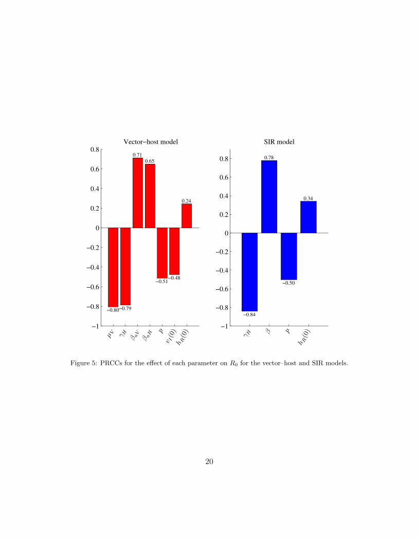
Because R0 is an important metric for an infectious disease, we performed uncer-tainty and sensitivity analysis of R0 for both models using partial rank correlationcoefficients (PRCC). The PRCC measures the independent effect of each input pa-rameter on R0, assuming the parameters to be independent [24]. The ordering ofthese PRCCs directly corresponds to the level of statistical influence, the impactthat uncertainty in the estimate of a parameter has on the variability of R0 [25]. Weused the “prcc” function of the R library epiR [26].

For both models, all of the parameters were significantly different from 0 (p-value <2.5×10−135). For the vector–host model, all parameters except hR(0) and vI(0) weremost influential in determining the magnitude of R0 (|PRCC| > 0.5), while only βand γH for the SIR model were most influential on the magnitude of R0. A positivePRCC value indicates that an increase in that parameter leads to an increase in R0,while a negative value shows that increasing that parameter decreases R0. For theparameters that appear explicitly in the R0 equations (2) and (5), the signs of thePRCCs were as expected. Of the remaining parameters, p and vI(0) have a negativeinfluence on R0, while hR(0) has a positive influence on R0.

Parameter estimates for both models suggest that the initial proportion of humansrecovered and the initial proportion of vectors infectious are very small. As a result,we tried fitting both models by fixing hR(0) = 0 and vI(0) = 2hI(0) and estimatingthe other parameters in order to decrease the complexity of the models (Figure 6).We fit the vector–host model by fixing hR(0) only, fixing vI(0) only and fixing bothhI(0) and vI(0). Similarly we fit the SIR model by fixing hR(0).

We used the Akaike Information Criterion (AIC) to compare the competing 6models (Table 2). The AIC is a measure of the relative goodness of fit of a statisticalmodel, balancing fit with number of parameters, finding the simplest model thatbest approximates the true, but unknown mechanisms generating the data. TheSIR model with fixed hR(0) had the minimum AIC value, implying this model wasthe best among the models. The difference in AIC between the best model andthe others (∆AIC) gave “considerably less support” for all the vector–host modelsand “substantial support” for both SIR models [27]. Alternatively, Akaike weights

9

provide the probability that a model is the best among the set of candidate models.The Akaike weight for the SIR model with fixed hR(0) gave 62% probability of itbeing the better model whereas the SIR model where hR(0) is also estimated was26% likely to be the better model. There was only a 12% probability that any of thevector–host models was best.

4. Discussion

The fitting of dengue incidence data from Thailand to simple vector–host and SIRmodel provided estimates of model parameters. The estimates of human recoveryrate from both the models suggest a recovery period of 2 to 7 days, which is consistentwith the estimates used in previous studies [2, 8]. The estimates of the probabilityof DHF from the vector–host model and the SIR model are that about 3 and 14out of 1000 infections develop into DHF, respectively for the two models. Based onthe annual number of dengue infections and DHF cases [2], 5 out of 1000 infectionsdevelop into DHF.

The ML estimate of the basic reproductive number (R0) for the SIR model is 30%smaller than the estimate for the vector–host model. This is driven by the recoveryrate (γH) being estimated as 68% larger in the SIR model. The MLE probability ofDHF (p) is 4.9 times larger for the SIR model. The two models—one with high R0

and low p, the other with low R0 and high p—both fit the data well. The PRCCresult showing a negative influence of p on R0 confirms the relationship between thesetwo parameters.

Dengue had been causing annual outbreaks in Thailand for some time prior tothe 1984 epidemic [5]. Despite this, our estimates of the initial proportion of peopleimmune (hR(0)) from both models are very small. A high birth rate [28] and thereemergence of dengue serotypes 3 and 4 [5] could explain this low immunity. Inaddition, mosquito seasonality may be important to explain the monthly variationin dengue incidence [6], and keeping the mosquito population constant for simplicityin our model could have contributed towards small estimates of hR(0).

The vector–host model fits the data slightly better than the SIR model, but thefewer number of parameters results in the SIR model being strongly selected by theAIC. Alternative measures for model selection like the Bayesian Information Cri-terion and the Deviance Information Criterion more strongly penalize the numberof parameters than AIC, so we expect the result of model selection to remain un-changed. This suggests that incorporating mosquito populations explicitly in denguemodels may not be necessary to estimate incidence.

We believe that for any vector-borne pathogen, explicitly including vector popu-lations may generally be unnecessary to model prevalence or incidence in human or

10

other primary host. We expect that models with and without explicit vectors willfit primary-host data about equally well and then the fewer parameters of the modelwithout explicit vectors will result in it being preferred by formal model selection.Other factors like seasonality in mosquito abundance may be crucial to fit somelong-term data (e.g. Figure 1), which could result in explicit-vector models fittingthe data significantly better than implicit-vector models. In addition, explicit-vectormodels are necessary when interventions are targeted at the disease vector, e.g. in-secticide or genetically modified mosquitoes. When the desired model output is theeffectiveness or cost-effectiveness of an intervention that acts on the primary host,our result suggests that implicit-vector models are likely to be sufficient.

The composite transmission parameter (β) for the vector–host model was ob-tained from the equilibria of the two models and may not be a good approximationfor our comparison of the dynamics of the models. This may explain the difference inthe estimates of the composite transmission parameter (β) between the two models.This is reinforced by the fact that the SIR model fits the observed data well, but notfor the same β values as the vector–host model. Thus, in addition to being preferredby model selection, use of the SIR model is justified when only the equilibrium valuesare of interest.

We chose to use DHF cases because the data was available monthly, while we areonly aware of annually reported DF cases [5]. Moreover, a person infected with DHFis more likely to visit hospital due to the severity of the disease, and so more likelyto be diagnosed and reported. Therefore, data on reported DHF cases may be moreaccurate to actual DHF cases than DF data is to DF cases.

We used a Bayesian MCMC technique for estimation, though other estimationmethods have also been used in the literature. In particular, least-squares error fittingis popular [e.g. 29] and the expectation maximization (EM) algorithm has seen someuse [30, 31]. We choose Bayesian MCMC approach as it provides a huge amount ofmodeling flexibility and enables analysis of all the model parameters or functions ofparameters. It also has advantage of providing a complete distribution for parametersas posterior distributions instead of point estimates. Moreover, posterior summariessuch as mean, medians, maximum likelihoods, maximum, minimum and credibleintervals are easy to obtain as well.

In this paper, we fitted dengue incidence data from Thaiand to vector–host andSIR models and obtained estimates of model parameters including average durationof dengue infection in humans, lifespan of mosquitoes and the probability of the severeform of disease. The parameter estimates were consistent with existing publishedvalues and PRCC values showed that all the parameters except initial conditions havesignificant influence on the magnitude of the basic reproduction number R0. Both the

11

vector–host model as well as the SIR model fit the incidence data well, however AICmodel selection found the SIR model with fixed hR(0) to be substantially better thanthe vector–host model, implying that incorporating mosquito population explicitlyin a dengue model may not be necessary to explain the incidence data from Thailand.

Acknowledgements

The authors thank Clemson University and Oregon State University for the fund-ing for this study.

References

[1] Center for Disease Control and Prevention, Dengue (Accessed January 14, 2013).URL http://www.cdc.gov/dengue/

[2] D. J. Gubler, Dengue and dengue hemorrhagic fever, Clin. Microbiol. Rev. 11 (3)(1998) 480–496.

[3] J. Medlock, P. M. Luz, C. J. Struchiner, A. P. Galvani, The impact of transgenicmosquitoes on dengue virulence to humans and mosquitoes, Am. Nat. 174 (4)(2009) 565–577.

[4] M. G. Guzman, G. Kouri, Dengue: an update, Lancet Infect. Dis. 2 (1) (2002)33–42.

[5] A. Nisalak, T. P. Endy, S. Nimmannitya, S. Kalayanarooj, R. M. Scott, D. S.Burke, C. H. Hoke, B. L. Innis, D. W. Vaughn, et al., Serotype-specific denguevirus circulation and dengue disease in Bangkok, Thailand from 1973 to 1999,Am. J. Trop. Med. Hyg. 68 (2) (2003) 191–202.

[6] H. J. Wearing, P. Rohani, Ecological and immunological determinants of dengueepidemics, Proc. Natl. Acad. Sci. U.S.A. 103 (31) (2006) 11802–11807.

[7] L. Esteva, C. Vargas, Influence of vertical and mechanical transmission on thedynamics of dengue disease, Math. Biosci. 167 (1) (2000) 51–64.

[8] D. A. T. Cummings, I. B. Schwartz, L. Billings, L. B. Shaw, D. S. Burke,Dynamic effects of antibody-dependent enhancement on the fitness of viruses,Proc. Natl. Acad. Sci. U.S.A. 102 (42) (2005) 15259–15264.

12

[9] Y. Nagao, K. Koelle, Decreases in dengue transmission may act to increase theincidence of dengue hemorrhagic fever, Proc. Natl. Acad. Sci. U.S.A. 105 (6)(2008) 2238–2243.

[10] B. Adams, E. C. Holmes, C. Zhang, M. P. Mammen Jr., S. Nimmannitya,S. Kalayanarooj, M. Boots, Cross-protective immunity can account for the al-ternating epidemic pattern of dengue virus serotypes circulating in Bangkok,Proc. Natl. Acad. Sci. U.S.A. 103 (38) (2006) 14234–14239.

[11] G. Chowell, P. Diaz-Duenas, J. C. Miller, A. Alcazar-Velazco, J. M. Hyman,P. W. Fenimore, C. Castillo-Chavez, Estimation of the reproduction number ofdengue fever from spatial epidemic data, Math. Biosci. 208 (2) (2007) 571–589.

[12] N. M. Ferguson, C. A. Donnelly, R. M. Anderson, Transmission dynamics andepidemiology of dengue: insights from age–stratified sero–prevalence surveys,Philos. Trans. R. Soc. Lond. B Biol. Sci. 354 (1384) (1999) 757–768.

[13] S. Cauchemez, F. Carrat, C. Viboud, A. J. Valleron, P. Y. Boelle, A BayesianMCMC approach to study transmission of influenza: application to householdlongitudinal data, Stat. Med. 23 (22) (2004) 3469–3487.

[14] Y. Huang, D. Liu, H. Wu, Hierarchical Bayesian methods for estimation ofparameters in a longitudinal HIV dynamic system, Biometrics 62 (2) (2006)413–423.

[15] J. S. Brownstein, T. R. Holford, D. Fish, Enhancing West Nile virus surveillance,United States, Emerg. Infect. Dis. 10 (6) (2004) 1129–1133.

[16] J. Reiczigel, K. Brugger, F. Rubel, N. Solymosi, Z. Lang, Bayesian analysis ofa dynamical model for the spread of the Usutu virus, Stoch. Environ. Res. RiskAssess. 24 (3) (2010) 455–462.

[17] Johns Hopkins Center for Immunization Research, Monthly incidence of DengueHemorrhagic Fever, 1983-1997, in 72 provinces of Thailand (Accessed January14, 2013).URL http://web.archive.org/web/20041216074102/http://www.jhsph.

edu/cir/dengue.html

[18] G. Macdonald, The Epidemiology and Control of Malaria, Oxford UniveristyPress, New York, 1957.

13

[19] M. N. Burattini, M. Chen, A. Chow, F. A. B. Coutinho, K. T. Goh, L. F. Lopez,S. Ma, E. Massad, Modelling the control strategies against dengue in Singapore,Epidemiol. Infect. 136 (3) (2008) 309.

[20] K. T. Alligood, T. D. Sauer, J. A. Yorke, Chaos: An Introduction to DynamicalSystems, Springer, New York, 1996.

[21] World Bank, Life expectancy at birth, total (years) (Accessed January 14, 2013).URL http://data.worldbank.org/indicator/SP.DYN.LE00.IN/countries/

TH-4E-XT?page=5&display=default

[22] M. J. Keeling, P. Rohani, Modeling Infectious Diseases in Humans and Animals,Princeton University Press, Princeton, 2008.

[23] H. W. Hethcote, The mathematics of infectious disease, SIAM Rev. 42 (4) (2000)599–653.

[24] S. M. Blower, H. Dowlatabadi, Sensitivity and uncertainty analysis of complexmodels of disease transmission: an HIV model, as an example, Int. Stat. Rev.62 (2) (1994) 229–243.

[25] M. A. Sanchez, S. M. Blower, Uncertainty and sensitivity analysis of the basicreproductive rate: tuberculosis as an example, Am. J. Epidemiol. 145 (12) (1997)1127–1137.

[26] M. Stevenson, epiR: An R package for the analysis of epidemiological data (Ac-cessed March 10, 2013).URL http://cran.r-project.org/web/packages/epiR/index.html

[27] K. P. Burnham, D. R. Anderson, Model Selection and Multimodel Inference:A Practical Information-Theoretic Approach, 2nd Edition, Springer, New York,2002.

[28] United Nations, World Fertility Data 2012 (Accessed March 25, 2013).URL http://www.un.org/esa/population/publications/WFD2012/

MainFrame.html

[29] A. Mubayi, C. Castillo-Chavez, G. Chowell, C. Kribs-Zaleta, N. Ali Siddiqui,N. Kumar, Transmission dynamics and underreporting of Kala-Azar in the In-dian state of Bihar, J. Theor. Biol. 262 (1) (2010) 177–185.

14

[30] S. Duncan, M. Gyongy, Using the EM algorithm to estimate the disease pa-rameters for smallpox in 17th Century London, in: Proceedings of the 2006IEEE International Conference on Control Applications, Omnipress, Madison,Wisconsin, 2006, pp. 3312–3317.

[31] M. Lavielle, A. Samson, A. Karina Fermin, F. Mentre, Maximum likelihoodestimation of long-term HIV dynamic models and antiviral response, Biometrics67 (1) (2011) 250–259.

15

1985 1990 19950

10

20

30

40

Year (1983−1997)

DH

F c

ase

s (t

housa

nds)

Figure 1: Monthly dengue hemorrhagic fever (DHF) incidence in Thailand from 1983 to 1997.

16

0 100 200 300 4000

5

10

15

Days (January 1984−March 1985)

DH

F c

ase

s (t

housa

nds)

Figure 2: Monthly DHF incidence in Thailand from January 1984 to March 1985.

17

0 100 200 300 400 5000

20

40

60

80

100

120

Days (January 1984−March 1985)

Cum

ula

tive D

HF

case

s (t

housa

nds)

Vector−host model

Observed data

Model with ML parameters

0 100 200 300 400 5000

20

40

60

80

100

120

140

160

180

Days (January 1984−March 1985)

SIR model

Figure 3: Fits of the vector–host and SIR models. Shown are the cumulative DHF cases from thedata (black circles), and from the models with the maximum–likelihood parameter estimates (thickblack curves) and 20 samples from the posterior parameter distribution (thin color curves).

18

0 0.2 0.40

0.1

0.2

βaH

(a)

0 1 20

0.05

0.1

βaV

(b)

0 10

0.05

0.1

β

(c)

0.2 0.4 0.60

0.05

γH

Rela

tiv

e f

req

uen

cy (d)

0 0.050

0.2

0.4

p

(e)

0 0.50

0.5

1

hR

(0)

(g)

Vector−host model

SIR model

0 0.050

0.5

1

vI(0)

(h)

2 4 60

0.05

0.1

R0

(i)

Figure 4: Posterior parameter densities for the vector–host and SIR models. (For the vector–hostmodel, β = βahβav/µv.)

19

−1

−0.8

−0.6

−0.4

−0.2

0

0.2

0.4

0.6

0.8

Vector−host model

0.71

0.65

0.24

−0.80−0.79

−0.51−0.48

µ V γ H β aV

β aH p

v I(0)

h R(0)

−1

−0.8

−0.6

−0.4

−0.2

0

0.2

0.4

0.6

0.8

SIR model

0.78

0.34

−0.84

−0.50

γ H

β p

h R(0)

Figure 5: PRCCs for the effect of each parameter on R0 for the vector–host and SIR models.

20

0 50 100 150 200 250 300 350 400 4500

10

20

30

40

50

60

70

80

Days (January 1984−March 1985)

Cum

ula

tive D

HF

case

s (t

housa

nds)

Observed data

Vector−host

Vector−host, vI(0) fixed

Vector−host, hR

(0) fixed

Vector−host, hR

(0) & vI(0) fixed

SIR

SIR, hR

(0) fixed

Figure 6: The maximum likelihood fits of models to the data.

21

PosteriorParameter Prior Model ML Median 90% CI

βaH(d−1

)U(0, 1) VH 0.0686 0.0521 (0.0146, 0.2241)

Mosquito-to-human transmission rate

βaV(d−1

)U(0.1, 2) VH 0.4307 0.4867 (0.1299, 1.6821)

Human-to-mosquito transmission rate

β(d−1

)U(0, 10)

VH 0.4881 0.4882 (0.2782, 0.9364)Composite transmission rate SIR 0.5718 0.3243 (0.1931, 0.5805)

γH(d−1

)U(0.1, 0.6)

VH 0.3104 0.2480 (0.1521, 0.4440)Human recovery rate SIR 0.5211 0.2650 (0.1347, 0.5315)p

U(0, 0.1)VH 0.0028 0.0022 (0.0010, 0.0086)

Probability of DHF SIR 0.0137 0.0057 (0.0018, 0.0354)

µH

(y−1

)1/69

VH — — —Human mortality rate SIR — — —

µV

(d−1

)U(0.01, 0.1) VH 0.0605 0.0531 (0.0378, 0.0781)

Mosquito mortality ratehR(0)

U(0, 1)VH 0.0067 0.0020 (0.0000, 0.1320)

Initial humans recovered SIR 0.0332 0.0019 (0.0000, 0.1363)vI(0)

U(0, 1) VH 0.0009 0.0005 (0.0000, 0.0056)Initial mosquitoes infectedR0 —

VH 1.5724 1.9733 (1.3556, 3.2059)Basic reproductive number SIR 1.0972 1.1989 (1.0523, 1.5243)

Table 1: Posterior summary of parameter estimates. For simplicity, µh was not estimated. R0 isnot a parameter, but rather a function of the other parameters. U(a, b) is the uniform distributionbetween a and b. For parameters common to both models, the same prior was used for both models.“ML” is maximum-likelihood estimate; “CI” is credible interval; “VH” is the vector–host model.Parameter units are given in parentheses.

22

Log- AkaikeModel df likelihood AIC ∆AIC weight

Vector–host 7 −0.0779 14.1559 7.7212 0.0130Vector–host, vI(0) fixed 6 −0.6847 13.3695 6.9348 0.0193Vector–host, hR(0) fixed 6 −0.1173 12.2346 5.7999 0.0341Vector–host, hR(0) & vI(0) fixed 5 −0.5835 11.1669 4.7322 0.0581SIR 4 −0.1020 8.2039 1.7692 0.2558SIR, hR(0) fixed 3 −0.2173 6.4347 0 0.6196

Table 2: Comparison of the vector–host and SIR models with and without fixed initial conditions.“df” is degrees of freedom, i.e. number of parameters.

23

Supplementary material for Comparingvector–host and SIR models for dengue

transmission

Abhishek Pandey∗ Anuj Mubayi† Jan Medlock‡

September 26, 2013

S1 Stability analysis of the vector–host model

For the vector–host model (1), scaling the state variables by their respective popu-lation sizes, to the proportions hS = HS/H, hI = HI/H, hR = HR/H, vS = VS/Vand vI = VI/V , gives the system of differential equations

dhSdt

= µH − βaHvIhS − µHhS,

dhIdt

= βaHvIhS − γHhI − µHhI ,

dhRdt

= γHhI − µHhR,

dvSdt

= µV − βaV hIvS − µV vS,

dvIdt

= βaV hIvS − µV vI .

(S1)

Using the next-generation method [1], the basic reproductive number is

R0 =βaHβaV

µV (µH + γH). (S2)

∗Department of Mathematical Sciences, Clemson University, Clemson, South Carolina 29634,USA†Department of Mathematics, Northeastern Illinois University, Chicago, Illinois 60625, USA‡Department of Biomedical Sciences, Oregon State University, Corvallis, Oregon 97331, USA

1

Because hS + hI + hR = 1 and vS + vI = 1, the reduced system

dhSdt

= µH − βaHvIhS − µHhS,

dhIdt

= βaHvIhS − γHhI − µHhI ,

dvIdt

= βaV hIvS − µV vI ,

(S3)

is equivalent to the full system (S1). This system is defined on the domain

Ω = (hS, hI , vI) : 0 ≤ vI ≤ 1, 0 ≤ hS, 0 ≤ hI , hS + hI ≤ 1. (S4)

A simple check shows that the vector field defined by model (S3) on the boundaryof Ω does not point to the exterior of Ω, so Ω is positively invariant under theflow induced by system (S3). This guarantees that the model numbers of humansand mosquitoes in the various epidemiological compartments never become negative,which is an obvious biological constraint.

The equilibrium points of system (S3) are

E0 = (1, 0, 0) and Ee = (h∗S, h∗I , v

∗I ), (S5)

where

h∗S =δ +M

δ +MR0

, h∗I =R0 − 1

δ +MR0

, v∗I =δ(R0 − 1)

(δ +M)R0

, (S6)

with

δ =βaVµV

and M =µH + γHµH

. (S7)

E0 is the disease-free equilibrium and Ee is the endemic equilibrium. For R0 < 1, E0

is the only equilibrium in Ω but the endemic equilibrium Ee also lies in Ω for R0 ≥ 1.The local stability of the equilibrium points is governed by the Jacobian matrix

DF =

−βaHvI − µH 0 −βaHhSβaHvI −(µH + γH) βaHhS

0 βaV − βaV vI −βaV hI − µV

. (S8)

2

S1.1 Disease-free equilibrium

The Jacobian matrix (S8) at E0 is

DF (E0) =

−µH 0 −βaH0 −(µH + γH) βaH0 βaV −µV

, (S9)

which has eigenvalues

− µH and−(µH + γH + µV )±

√(µH + γH + µV )2 − 4µV (µH + γH)(1−R0)

2.

(S10)All of the eigenvalues have negative real part for R0 < 1 and so E0 is locally asymp-totically stable for R0 < 1.

To show global stability of E0, we consider the Lyapunov function on interior ofΩ

Λ =βaHµV

vI + hI (S11)

which has orbital derivative

dΛ

dt=βaHµV

dvIdt

+dhIdt

= −βaH(1− hS)vI − (µH + γH)[1−R0(1− vI)]hI .(S12)

For R0 ≤ 1, the orbital derivative dΛdt≤ 0 in Ω and the subset of Ω where dΛ

dt= 0 is

given by(1− hS)vI = 0 (S13)

and

hI = 0 if R0 < 1,

hIvI = 0 if R0 = 1.(S14)

Thus E0 is the only invariant set contained in dΛdt

= 0. Also, the interior of Ω isbounded. Therefore, E0 is locally stable and all trajectories starting in Ω approachE0 as t → +∞ [2, p. 317, Corollary 1.1]. This establishes the global asymptoticstability of E0 for R0 ≤ 1.

For R0 > 1, the eigenvalue

−(µH + γH + µV ) +√

(µH + γH + µV )2 − 4µV (µH + γH)(1−R0)

2> 0, (S15)

so E0 is unstable.

3

S1.2 Endemic equilibrium

As R0 increases through 1, the disease-free equilibrium E0 becomes unstable and theendemic equilibrium Ee moves from outside to inside Ω. The Jacobian matrix at Eeis

DF (Ee) =

−µHδ+MR0

δ+M0 −µHMR0

δδ+Mδ+MR0

µHM(R0−1)δ+M

−µHM µHMR0

δδ+Mδ+MR0

0 µV δR0

δ+MR0

δ+M−µVR0

δ+Mδ+MR0

. (S16)

The characteristic polynomial of matrix (S16) is

p(λ) = λ3 + Aλ2 +Bλ+ C, (S17)

where

A = µHδ +MR0

δ +M+ µHM + µVR0

δ +M

δ +MR0

B = µ2HM

δ +MR0

δ +M+ µV µHR0 +

µHµVM(R0 − 1)δ

δ +MR0

C = µ2HµVM(R0 − 1).

(S18)

For R0 > 1, the coefficients A, B, and C are positive and

AB > µ2HµVMR0 > C, (S19)

so the characteristic polynomial (S17) satisfies the Routh–Hurwithz conditions [3].Therefore, Ee is locally asymptotically stable.

S2 Comparing equilibria of the vector–host and

SIR model

The endemic equilibrium (S6) for the vector–host model has

h∗S =δ +M

δ +MR0

=1 + µH

βaHR0

R0 + µHβaH

R0

,

h∗I =R0 − 1

δ +MR0

= (R0 − 1)µH

(µH + γH)(R0 + µH

βaHR0

) . (S20)

IfµHβaH

R0 1, (S21)

4

as is true of our ML estimates, then since R0 > 1,

h∗S ≈1

R0

,

h∗I ≈ (R0 − 1)µH

(µH + γH)R0

= (R0 − 1)µHβ,

(S22)

where

β =βaV βaHµV

, (S23)

which is exactly the endemic equilibrium of the SIR model (3).

S3 Detailed explanation of the Bayesian MCMC

method

Given a mathematical model, the aim is to find the distribution of the unknownparameter values θ for the model that are consistent with the data D. In our case,the data are a time series of monthly cumulative incidence, and yi(θ) = HC(ti)/His the time series produced by the model at the same monthly time points ti as thedata. We used the least-squares error function

E2 =∑i

(Di − yi(θ)

)2

(S24)

to calculate the distance between the model output and the data. We assumed thatthe error function obeys a normal distribution with zero mean and variance 1/2:

Pr(E2)∝ exp

(−E2

). (S25)

This is the likelihood function of the parameters given the data,

L(θ) = Pr(D | θ) ∝ exp(−E2

). (S26)

Once the prior distribution Pr(θ) for the unknown parameters is defined, theprobability of parameters given the data points, i.e. the posterior distribution, isgiven by Bayes’s Theorem,

Pr(θ | D) =Pr(D | θ) Pr(θ)

Pr(D), (S27)

5

where Pr(D | θ) is the likelihood function (S26) and Pr(D) is called the evidence,which is the integral of the likelihood over the prior distribution of the parameters:

Pr(D) =

∫Pr(D | θ) Pr(θ) dθ. (S28)

It is difficult to compute Pr(D), but we can instead use

Pr(θ|D) ∝ Pr(D|θ) Pr(θ) (S29)

to find the posterior parameter distribution.Using Bayes’s Theorem (S29), we form a Markov chain which asymptotically

converges to the posterior parameter distribution by using the Metropolis Algorithm.The Metropolis Algorithm is an iterative procedure that uses an acceptance–rejectionrule to converge to the required distribution [4]. The algorithm is:

1. Start with some initial guess for the parameter values. We randomly chose astarting point θ0 from the prior distribution Pr(θ).

2. For each iteration n = 1, 2, 3, ......

(a) A new proposed set of parameter values is generated by sampling θ∗

from the proposal distribution J (θ∗ | θn−1). The proposal distributionJ (θ∗ | θn−1) must be symmetric, i.e. J (θ∗ | θn−1) = J (θn−1 | θ∗), for thisalgorithm.

(b) Using the likelihood function, the ratio

r = min

Pr(θ∗ | D) Pr(θ∗)

Pr(θn−1 | D) Pr(θn−1), 1

(S30)

is calculated.

(c) We generate a random uniform number between 0 and 1 and call it α.Then the parameter values for this iteration are

θn =

θ∗ if α < r,

θn−1 otherwise.(S31)

This algorithm must be run for enough iterations for the parameter values toconverge to the posterior distribution. There are several convergence diagnosticswhich can be employed to detect whether the chain has converged [5]. We used the

6

Gelman–Rubin test [6] for the convergence diagnostic of our simulations, which isbased on multiple independent simulated chains. The variances within each chainare compared to the variances between the chains: large deviation between these twovariances indicates non-convergence.

The posterior is insensitive to the choice of proposal density, J(θ∗ | θn−1), but thenumber of iterations until the chain converges may be heavily affected. It is difficultto choose an efficient proposal distribution, but normal distributions have been foundto be useful in many problems [4]. We used a multivariate normal distribution withmean θn−1 and covariance λ2Σ as our proposal distribution,

J(θ∗ | θn−1

)∼ N

(θn−1, λ2Σ

). (S32)

For the multivariate normal proposal distribution, for optimal convergence, proposalsshould be accepted at a rate of 0.44 in one dimension and 0.23 in higher dimensions[4]. To achieve this, we used a variant of the Metropolis Algorithm that updatesthe covariance matrix Σ and the scaling factor λ of the proposal distribution afterevery 500 iterations. We initially chose the covariance to be the d×d identity matrix(Σ0 = I) and the initial scaling factor to be λ0 = 2.4/

√d, where d is the number

of parameters being estimated. After every 500 iterations, the covariance matrix isupdated by

Σk = pΣk−1 + (1− p)Σ∗ (S33)

where Σ∗ is the covariance of the last 500 parameter values and p = 0.25 is theweight given to the old covariance matrix. Similarly, the scaling factor is updatedusing the Robbins–Monro algorithm [7],

λk = λk−1 exp

(α∗ − αk

), (S34)

where α∗ is the acceptance rate for the last 500 iterations and the target acceptancerate is

α =

0.44 for d = 1,

0.23 for d > 1.(S35)

We ran the adaptive algorithm in two phases: first, the adaptive phase, which isrun until the Gelman–Rubin convergence test passed, and then the fixed phase, wherethe algorithm is run to sample from the posterior distribution without updating thecovariance matrix and the scaling factor. Samples from the only last phase were usedin the final inferences.

7

References

[1] O. Diekmann, J. A. P. Heesterbeek, M. G. Roberts, The construction of next-generation matrices for compartmental epidemic models, J. R. Soc. Interface7 (47) (2010) 873–885.

[2] J. K. Hale, Ordinary Differential Equations, John Wiley & Sons, New York, 1969.

[3] F. Brauer, C. Castillo-Chavez, Mathematical Models in Population Biology andEpidemiology, Springer, New York, 2001.

[4] A. Gelman, J. B. Carlin, H. S. Stern, D. B. Rubin, Bayesian Data Analysis, 2ndEdition, Chapman & Hall/CRC, Boca Raton, 2004.

[5] M. K. Cowles, B. P. Carlin, Markov chain Monte Carlo convergence diagnostics:a comparative review, J. Am. Statist. Ass. 91 (434) (1996) 883–904.

[6] A. Gelman, D. B. Rubin, Inference from iterative simulation using multiple se-quences, Stat. Sci. 7 (4) (1992) 457–472.

[7] H. Robbins, S. Monro, A stochastic approximation method, Ann. Math. Stat.22 (3) (1951) 400–407.

8