Comparing the Consistency of Price Parities for Regions of ... · In our previous RPP estimates, we used the only the CPI data, that is, the Rents and Owners’ Equivalent Rent observations

Comparing the Consistency of Price Parities for Regions of the U.S. in an Economic Approach Framework

Bettina Aten and Marshall Reinsdorf*

U.S. Bureau of Economic Analysis Email addresses: [email protected], [email protected].

Presented at the 31st General Conference of IARIW St. Gallen, Switzerland

Session 7C: Price Comparisons I

August 27, 2010

* This work was made possible by an interagency agreement and the collaboration of the Bureau of Labor Statistics (BLS), the Census Bureau, and the Bureau of Economic Analysis (BEA). The agreements provided access to the micro-data in the CPI (Consumer Price Index) survey and in the ACS (American Community Survey). We are grateful to the BLS Division of Prices and Index Number Research, and to Walter Lane, Frank Ptacek, Robert Cage, and Joshua Klick in the CPI Division. We also thank the support of the Housing and Household Economic Statistics Division of the Census Bureau, particularly David Johnson for his unflagging encouragement, as well as Trudi Renwick and Ali Bishaw for their help. Special thanks to Lyuba Rosenthal (BLS) and Roger D’Souza (BEA) for their excellent programming skills and analytical support. Finally, we would like to thank the organizers and participants of the Conference on International Comparisons of Prices, Income and Productivity at the University of Oxford, England, on April 8-9, 2010, for comments and suggestions on earlier versions of this paper.

1. Introduction

Real comparisons of incomes1 generally imply either (1) an adjustment of nominal incomes for price changes over time, that is, an adjustment to separate volume from price changes, or (2) an adjustment for relative price differences across space, or a purchasing power parity adjustment. If both those adjustments exist for a set of geographic entities and time periods, the question then becomes one of obtaining a measure that is consistent across both space and time. Feenstra, Ma and Rao (2009), and Rao, Rambaldi and Doran (2008) have recently looked at ways of obtaining this space-time consistency in the international context, while others such as Oulton (2008), Neary (2004), have developed approaches that shed light on the properties of both chained and cost-of-living approximations to price indexes, respectively. Studies go back much further to Kravis, Heston and Summers (1982), Varjonen (2001), Dalgaard and Sorensen (2002), and Schreyer and Koechlin (2002), who faced the practical problems of reconciling benchmark purchasing power parities (PPPs) with national accounts growth rates. In the regional context, Gong and Meng (2008) derive price differences in urban China for 1986-2001. They use the Chinese CPI series and unit values from a household expenditure survey, while Hawkes (1998) and Silver (2004) use scanner data to identify some of the underlying issues. This paper uses regional price and expenditure data to explore the space-time consistency question for the U.S. for the years 2005-2008 and a set of 38 geographic areas. We estimate a number of traditional multilateral price indexes, as well as a demand model extension developed by Neary (2004) and termed the ‘Geary Allen International Accounts’ or GAIA system. The traditional and the GAIA multilateral indexes allow us to convert nominal regional income values measured at national prices into regional incomes at regional prices. Currently, the only official measure of regional real incomes in the U.S. is based on national prices, and there are also no constant price income time series at the regional level, in part because of the instability of the sub-national inflation adjustments.2 Our intended use of the multilateral price indexes in comparing real personal incomes of regions does not necessarily imply the use of the cost-of-living index concept embodied in

1 Ultimately, we would like to adjust household incomes, but for this exercise, we are in fact using only expenditure data, so our reference to incomes is a loose one, referring neither to total GDP nor total income, but simply to total consumption expenditures. 2 BLS discourages the use of sub-national CPIs for indexation (see http://www.bls.gov/cpi/cpifaq.htm#Question_18). For research purposes only, alternative CPI series at the 38 area level are available.

the GAIA indexes. Nevertheless GAIA indexes offer certain advantages that make them a worthwhile alternative for us to consider. One advantage of the GAIA method is that it sheds light on the problem of lack of correspondence between changes from year to year in our estimates of the areas’ RPPs and changes in their CPIs. In particular, the GAIA has the potential to model the degree to which non-homothetic preferences (income effects) are responsible for deviations of the areas’ CPI changes from the changes in their Geary RPPs. GAIA indexes also have the convenient additive properties of the Geary method without incurring the Geary method’s disadvantage of being prone to distortion from Gerschenkron effects (Gerschenkron [1947], Jonas and Sardy [1970]). When the volumes of consumption of two countries are compared, each country’s relative volume of consumption tends to be shown as higher if the prices of the other country are used to value the two countries’ consumption baskets than if its own prices are used. This is known as the Gerschenkron effect. It occurs because the relative quantity consumed of a commodity is generally higher in the country where its price is lower. The same sort of bias exists when countries’ relative price levels are compared, where relative price levels are measured using the ratio of a purchasing power parity (PPP) exchange rate to the market exchange rate. The relative price level comparison will generally imply a lower price level for a country if its own consumption basket is used for the comparison than if the other country’s basket is used, because things consumed in relatively greater quantities in the other country are likely to have low prices there. Multi-lateral comparisons using the Geary method are also susceptible to Gerschenkron effects because the Geary world price vector often reflects either the structure of prices in the largest economy or their structure in a large block of similar economies. In either case, the relative volume of consumption in the countries whose prices most closely resemble the Geary world prices tends to be understated because of Gerschenkron effects. The GAIA method avoids this problem by substituting the commodity baskets that would be predicted to occur if each country faced the world prices for the commodity baskets that actually occur. This helps to avoid distortions caused by high relative consumption of commodities with low prices in countries whose price structure differ greatly from that of the world prices. The starting point of our estimates is a set of spatial price relatives for 207 consumption goods and services in the CPI (Aten and D’Souza 2008) and their corresponding weights in the Consumer Expenditure Survey. These spatial price relatives originate from direct price observations, and are uniquely identified by a set of characteristics, including the geographic area in which they are sampled. Section Two describes the estimation of an aggregate multilateral price index, or overall Regional Price Parity (RPP), for each area and each time-period, based on the detailed price relatives and expenditure weights.

Section 2 has two parts. Part a) describes the price-related data for housing costs in the RPPs using two sources of data. One is the CPI itself, called Rents and Owners’ Equivalent Rents (henceforth ROER), while the other is the American Community Survey (ACS), produced by the Census Bureau. The housing component of the ACS survey also contains information on rents and on the monthly owner costs (henceforth RMOC), but does not impute owners’ equivalent rents as in the BLS data. One of the advantages of the ACS survey is its scope and geographic representation. Unlike the BLS, it covers all metropolitan and non-metropolitan counties, including rural counties, but does so over a multi-year period. For example, the 3-year ACS includes all geographic areas with a population of 20,000 or more, while the 5-year ACS includes area with a population less than 20,000. It is more comprehensive than the BLS housing survey, but less timely: the first 2005-2009 estimates will be released in late 2010. In Part b) of Section 2 we explain how we aggregate the price and expenditure data into sub-aggregate headings, such as Food, Goods, Services and Rents, and also into an overall RPP. These sub-aggregate headings are needed in Section 3 to examine differences in demand with explicit assumptions about tastes using Deaton and Muellbauer’s (1980) demand system and the GAIA method. In Section 4 we bring in the time-dimension and look at the consistency of the estimates by comparing the benchmark RPPs from estimates extrapolated using the chained and the fixed-weight Consumer Price Index (CPI) for the 38 areas.

2. Regional Price Parities (RPPs) RPPs are multilateral or spatial price indexes and refer to aggregates of consumption goods and services. The CPI survey compiles detailed price observations and sampling quote weights representing the consumption purchases of approximately 87% of the U.S. population. Given these price quotes, we first obtain estimates of the price parities for various categories of expenditure, such as Flour, Women’s Suits, Men’s Haircuts and New Cars. There are 207 such categories, known as Item Strata in the CPI, or Basic Headings in the International Comparison Program. For items with large expenditures, such as New Cars, a hedonic regression is estimated, with the outlet type, and other item characteristics as independent variables, and a dummy for each area. For many of the smaller expenditures, generally comprising less than 2% of an area’s expenditure, a simpler method is used, known as the Country Product Dummy (CPD), (Summers, 1973). The CPD is a regression with dummy variables for the areas and when possible, controlling for other quality differences such as the outlet type and the product type. It is weighted (as are the more detailed hedonic regressions), with weights equal to the probability sampling quote weights. The description of the hedonic regressions and the CPD methodology for obtaining these 207 item strata price parities is in Aten (2005, 2006).

2a) Housing or Shelter Costs Two of the 207 items in the CPI refer to the costs of Housing, or Shelter. One is for actual Rents paid by renters and the other for Owners’ Equivalent Rents, or the rent imputed for owner-occupied homes (see Poole, Ptacek and Verbrugge [2005], the BLS Handbook of Methods [1992], and Lane and Sommers [1984]). These two items make up about 30% of average household expenditures in the Consumer Expenditure (CE) Interview Survey3 . In our previous RPP estimates, we used the only the CPI data, that is, the Rents and Owners’ Equivalent Rent observations (ROER) from the BLS, together with the other goods and services. Here we introduce another source of data, just for housing costs: the multi-year ACS survey, with Rents and Monthly Owner Costs (RMOC), from the Census Bureau. One reason for comparing these two sources is that the relative cost of housing or shelter is hard to measure, both in terms of available data, and in terms of competing approaches to imputing home-owner relative costs. The two data sources are discussed briefly below.

1. ROER The ROER observations, like the rest of the CPI, are designed to measure changes in prices over time, and contain approximately 34,000 observations on occupied housing units per year on a rotating-6 month schedule4. We run two sets of regression models, one for Rents, and the other for Owners´ Equivalent Rents. The regressions (Aten, 2005), are sensitive to different specifications, although the area coefficients are relatively stable from year to year. Their predicted values at the means5, and their standard errors are shown in Appendix Table A1. One advantage of using the CPI housing costs is that they are available on a timely basis (soon after the end of the calendar year, as are the other good and items in the CPI). A second advantage is that there are more characteristics recorded per observation, for example, the number of bathrooms and the length of occupancy of the rental unit. The disadvantage, for spatial comparisons, is that there are few observations per area once we control for various characteristics, resulting in high leverage points and larger variances when compared to the ACS data from Census.

3 http://www.bls.gov/bls/fesacp1120905.pdf 4 http://www.bls.gov/cpi/cpifact6.htm 5 In SAS, these are the marginal or least squares means, referring to the group means after having controlled for the covariates. (see http://support.sas.com/onlinedoc/913/getDoc/en/statug.hlp/glm_sect34.htm )

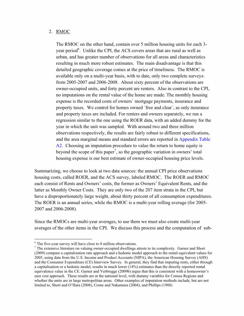
2. RMOC The RMOC on the other hand, contain over 5 million housing units for each 3-year period6. Unlike the CPI, the ACS covers areas that are rural as well as urban, and has greater number of observations for all areas and characteristics resulting in much more robust estimates. The main disadvantage is that this detailed geographic coverage comes at the price of timeliness. The RMOC is available only on a multi-year basis, with to date, only two complete surveys: from 2005-2007 and 2006-2008. About sixty percent of the observations are owner-occupied units, and forty percent are renters. Also in contrast to the CPI, no imputations on the rental value of the home are made. The monthly housing expense is the recorded costs of owners´ mortgage payments, insurance and property taxes. We control for homes owned ´free and clear´, as only insurance and property taxes are included. For renters and owners separately, we run a regression similar to the one using the ROER data, with an added dummy for the year in which the unit was sampled. With around two and three million observations respectively, the results are fairly robust to different specifications, and the area marginal means and standard errors are reported in Appendix Table A2. Choosing an imputation procedure to value the return to home equity is beyond the scope of this paper7, so the geographic variation in owners’ total housing expense is our best estimate of owner-occupied housing price levels.

Summarizing, we choose to look at two data sources: the annual CPI price observations housing costs, called ROER, and the ACS survey, labeled RMOC. The ROER and RMOC each consist of Rents and Owners’ costs, the former as Owners’ Equivalent Rents, and the latter as Monthly Owner Costs. They are only two of the 207 item strata in the CPI, but have a disproportionately large weight, about thirty percent of all consumption expenditures. The ROER is an annual series, while the RMOC is a multi-year rolling average (for 2005-2007 and 2006-2008). Since the RMOCs are multi-year averages, to use them we must also create multi-year averages of the other items in the CPI. We discuss this process and the computation of sub-

6 The five-year survey will have close to 8 million observations. 7 The extensive literature on valuing owner-occupied dwellings attests to its complexity. Garner and Short (2009) compare a capitalization rate approach and a hedonic model approach to the rental equivalent values for 2005, using data from the U.S. Income and Product Accounts (NIPA), the American Housing Survey (AHS) and the Consumer Expenditure (CE) Interview Survey. In general, they find that imputing rents, either through a capitalization or a hedonic model, results in much lower (14%) estimates than the directly reported rental equivalence value in the CE. Garner and Verbrugge (2009b) argue that this is consistent with a homeowner’s user cost approach. These results are at the national level, with dummy variables for Census Regions and whether the units are in large metropolitan areas. Other examples of imputation methods include, but are not limited to, Short and O’Hara (2008), Crone and Nakamura (2004), and Phillips (1988)

aggregate headings and the overall RPPs below. Part of the motivation for examining both sources of housing or shelter data is our need for consistency and stability over time. We address this question in Section Four in more detail.

2b) Sub-Aggregate Headings BLS uses data from the Consumer Expenditure (CE) Survey to estimate budget shares for the 207 item strata used in the CPI for each of the 38 geographic areas. The CE surveys rural areas, and estimates expenditures on Medical Insurance, but since these are not in the CPI survey, they are not included in the RPPs. Also, as there are no expenditure weights below the item strata level8, or for a finer level of geography, we are constrained to estimating aggregate RPPs for 38 areas. The aggregation techniques for multilateral price indexes are borrowed from the international literature on purchasing power parities (PPPs) (see for example, Summers and Heston [1991], Heston and Lipsey [1999], Diewert [1993, 1999], Rao [2009], Deaton and Heston [2009]). In the international context, aggregate country PPPs are estimated at the level of GDP and for major expenditure headings, based on prices and expenditure distributions available from national statistical offices and international agencies and programs, such as Eurostat, the OECD (2006), and the World Bank (2010) International Comparison Program (ICP). We will make estimates for only the top level of aggregation, total expenditures. However, these expenditures are only for personal consumption, and exclude the other components of GDP. In addition, for inputs into the GAIA multilateral aggregation method, we must estimate sub-aggregate RPPs for expenditure headings. We would like to explore the economic relationships in a demand model for all 207 items, but with only 38 areas, we are limited in our choice of models by the degrees of freedom.9 We therefore begin by consolidating the 207 item strata into fewer categories, corresponding to groupings that might make sense in terms of consumption habits and differences in spatial prices. A justification for this comes from Kravis, Heston and Summers or KHS, (1982), Chapter 9, which discusses tastes and revealed preferences in the context of a demand analysis for 34 countries. KHS suggest that tastes at higher levels of aggregation, such as food, clothing and shelter, might be similar, 8 There are quote weights below the item stratum level, but they refer to the adjustment in the probability sampling procedure of the CPI. 9 Oulton (2008) suggests an alternative method in a time-series context where a set of principal components, rather than an aggregate grouping, is used in the system. We began to explore this approach here, but found that it took 27 components to account for 90% of the variance in the 207 relative prices using the correlation matrix, and 24 components using the covariance matrix. Given that we only have 38 areas, we feel that 10 components is probably the maximum. The 10 components would account for only 60% of the cumulative variation. The principal components approach could be further researched in the time-series context.

“but with food or clothing or shelter requirements being satisfied in different ways in different countries” (p.347). Their results using a linear expenditure system indicate that their proposition is supported “for most practical purposes”. In the case of the U.S., we would expect even stronger results, as differences in the quantities of goods and services consumed across urban and metropolitan areas are likely to be more similar than for example, between India and Poland. We choose four groupings: Food, Goods (other than Food), Housing or Shelter costs (ROER and RMOC) and Services10. Housing (or shelter) is treated as a separate category because both ICP studies (KHS 1982) and studies of areas within the US (Aten 2005, p.27) show that the spatial dispersion of prices of services is much greater than that of goods, and that within services, housing costs for Rents and Owners’ Equivalent Rents vary more than other services. When we aggregate the price relatives into groupings for four or more headings, or at the aggregate level for the overall price parity, the results must retain the fundamental properties of a multilateral price index: reciprocity and transitivity. Deaton and Heston (2009) and Balk (2009) provide full accounts of these properties and of how they are attained by the four ‘traditional’ multilateral aggregation formulas considered here:

(1) the Törnqvist based Gini-EKS, (2) the Fisher Gini-EKS (3) the Weighted CPD, (4) and the Geary method (also known as the Geary-Khamis, or GK, method).11

Only one of these traditional aggregation methods, the Geary method, is additive. That is, the Geary sub-aggregate price parities and expenditures may be added up to the overall price parity. Additivity is a very convenient property, but it is generally not considered essential in a framework for multilateral comparisons.12 The sequence of our estimation is as follows. First calculate the Geary national average price (πn) for each of the 207 items, along with the overall price parity (RPP) for each area.13

10 In earlier work, we presented more groupings: subdividing Food into At Home and Away from Home, and adding Gasoline to form six categories. Available from the authors are eight groups: separating Automobiles and Alcohol & Tobacco categories from the Good categories. Beyond eight, there are too few degrees of freedom for meaningful estimates with 38 areas. 11 See also Gini [1924], Eltetö and Köves [1964], Szulc [1964], Diewert [1976, 2001] , Summers [1973], Rao [2004], Geary [1958] and Khamis [1972]. There are other formulas for multilateral aggregations, such as the Iklé (1972), the Minimum Spanning Tree method (Koves [1983], Hill [1999]), the CKS (Commensurable Kurabayashi-Sakuma) method (Sakuma, Rao and Kurabayashi 2009) and the SS (Standardized Structure) method (Sergueev 2009). They bear consideration for future research. 12 As evidenced by the use of non-additive price indexes in Eurostat and the OECD. 13 The solution is obtained iteratively from the following equations:

Next calculate the expenditure on each item in each area measured at the item’s national price. 14 These calculated expenditures at national prices are then summed for the desired groupings (such as Food). The ratio of expenditures on Food at an area’s own prices to the expenditures at national prices is equal to the area’s price parity for Food, and similarly for the other groupings. Finally, the price parities for each area-grouping cell are used as the inputs for the demand model in the GAIA system, along with the nominal shares (at own area prices), and the per capita total ‘real’ expenditures. There are a number of options for the sub-aggregate price parities and per capita ‘real’ expenditures inputs to the demand model. We have chosen the Geary method, but another multilateral method, such as one of the variants of the Gini-EKS method, could be used. Similarly, various price indexes exist that are suitable for deflating total per capita nominal expenditures into the initial ‘real’ expenditures of the demand model. The Geary, Gini-EKS (Törnqvist and Fisher approaches) and the Weighted CPD are candidates.15 So is a Stone-type (1953) index derived simply as the share-weighted average of the price parities, where the weights are the national averages of the nominal shares. We use the Stone index, but it seems to make little difference what the starting point is, as the final estimates are obtained iteratively as discussed in Section 3. The Geary national average prices (πn; n=1 to 4) for the annual and multi-year averages for the four sub-aggregates of Food, Goods, Shelter Costs and Services are shown in Table 1a. The columns labeled 2005 through 2007 are for the annual CPI only data, using the ROER series, while the columns 2005-2007 and 2006-2008 are the multi-year averages with the ROMC housing cost data from the ACS. The weighted average across the four items equals 1 in each year by construction.

( )

for n 1... items

( )for a 1... areas

na

a an

naa

nan

an na

n

pqRPP

Nq

pqRPP A

q

π

π

⎛ ⎞⎜ ⎟⎜ ⎟= =⎜ ⎟⎜ ⎟⎝ ⎠

⎛ ⎞⎜ ⎟= =⎜ ⎟⎜ ⎟⎝ ⎠

∑∑

∑∑

14 We follow KHS (1982) and use the term ‘notional’ quantity to denote expenditures at area’s own prices divided by the initial own area item price relatives. When multiplied by the national average prices (the π’s), these notional quantities are the expenditures at national prices. The ratio of an area’s total expenditures at own prices to its total expenditures at national prices is the area’s relative price parity (RPP). The total of all expenditures (across areas and items) is the same at national and area-specific prices, so that the overall national RPP is equal to one. 15 Their formulas are given in the Appendix.

For reference, the national average prices for Shelter (π3) using the annual ROER more closely resemble those of Minneapolis in 2005, Denver in 2006, Tampa in 2007 and Portland in 2008, while when using the multi-year ROMC, they more closely resemble those of Minneapolis for both periods. If the average prices and expenditures were dominated by very high cost Shelter areas, then the national Geary averages (πn) would tend towards these higher levels, and there would be a greater likelihood of a Gerschenkron-type effect, with an overestimate of the price parities for Shelter in the very inexpensive areas. However, Minneapolis, and Denver, Tampa and Portland are in the middle rather than at the high end of Shelter costs. Chart 1 shows the 2005 Geary price averages at the national level and for a few of the areas. In the next section, we describe the steps in the GAIA estimation: first, we specify a demand model and obtain its parameters, then re-estimate Geary with the predicted values to obtain the final GAIA national price parities for the commodity groupings and the overall RPPs.

3. The GAIA Method To implement Neary’s (2004) GAIA method, we replace the ‘notional’ quantities in the Geary formula with a set of ‘virtual’ quantities. Notional quantities refer to nominal expenditures divided by input prices, and are expressed in dollar terms, not in physical quantities. These notional quantities enter the Geary method as weights, and are ‘fixed’ in the sense that the areas with the largest weights will have greater influence on the resulting price parities. This can lead to a Gerschenkron effect if some areas are much larger than the others. If, for example, we were only comparing large, high rent cities with small, low rent areas, the Geary system would overestimate the price parity for rents in those smaller areas, and hence underestimate their overall RPPs, making the smaller areas look better off in ‘real’ terms than they actually were (assuming the relative prices of other goods were similar).16 In the case of the US areas, it is not clear a priori whether the large cities are dominant enough to cause a significant Gerschenkron effect, as the sampling frame for expenditures is more evenly spread across the country, and prices are more homogenous across the areas of the US than across the world. As mentioned in the previous section, the average prices, for Shelter costs resemble those of middle-income areas such as Denver and Minneapolis, rather than a higher income area such as New York City or San Francisco.

16 In the ICP, this problem was more pronounced when a smaller subset of the world’s countries was sampled. As the ICP has grown to include countries like China and India, the argument that the price parities more closely resembled a high-income country than any middle-income country no longer holds.

The GAIA system uses the expenditure shares and quantities that are estimated to be chosen at world prices taking into account substitution behavior across groups of goods. It therefore approximates a cost-of-living index framework. If we are to compare results over time, as we would like to in the long-run, the GAIA framework is more consistent with a chain-type price index series, such as the C-CPI-U of the Bureau of Labor Statistics. This we examine more closely in Section 4. To estimate the expenditure shares and quantities of the GAIA system, we fit the nonhomothetic “almost ideal” (AI) demand system of Deaton and Muellbauer (1980). The theoretical AI system imposes three sets of constraints on the AI demand system coefficients (shown in the Technical Appendix) so that the demand system will satisfy the homogeneity and Slutsky matrix symmetry restrictions of economic theory. Estimation of this constrained version of the AIDS model begins with Stone’s price index, calculated as the simple weighted geometric mean of the input prices, where the weights are the average weights for the country. We then impose homogeneity and symmetry in the price coefficients and use an iterative Seemingly Unrelated Regression (SUR) procedure to obtain the parameter estimates. The Stone index is then replaced with a new index P evaluated with the values of the estimated parameters.17 The process is repeated until the system converges.18 The GAIA national prices (πn) for the annual and multi-year averages are shown in Table 1b. Unlike the prices in Table 1a, these are calculated using estimated demand model parameters. The demand model was estimated at the four grouping level (Food, Goods, Rents: ROER and RMOC, and Services). As expected, the demand model predicts some substitution across the groups, so that the range of national average prices will be smaller.

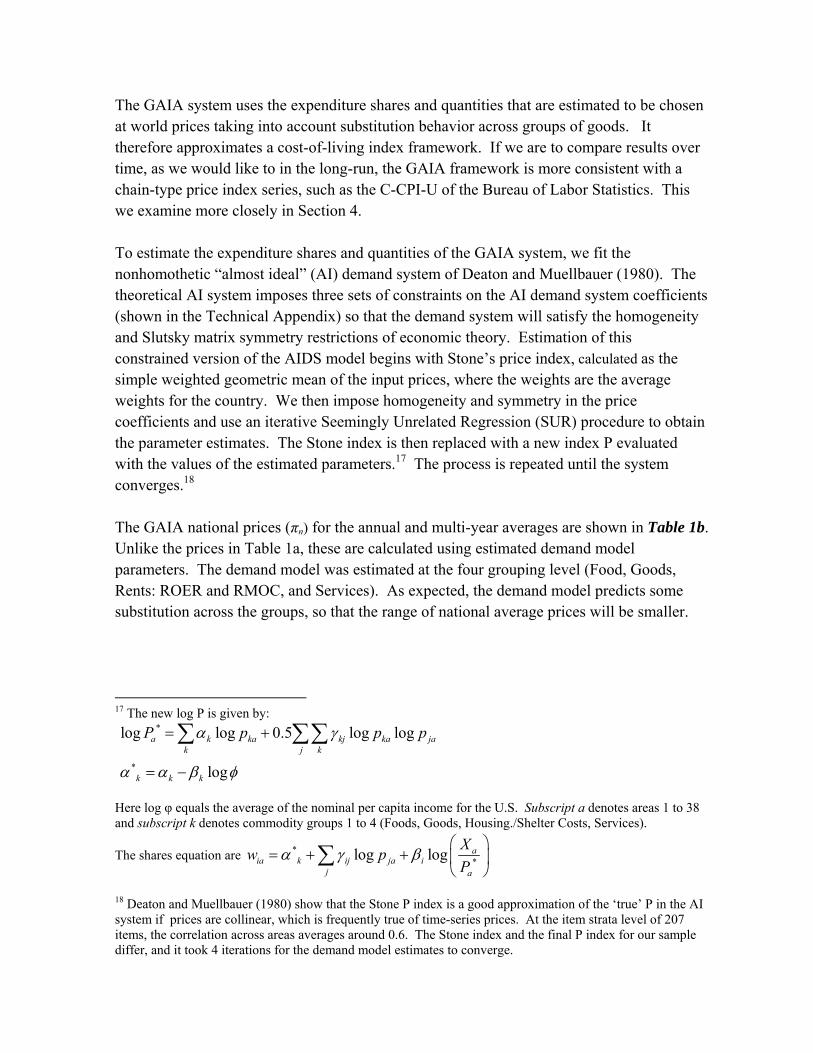
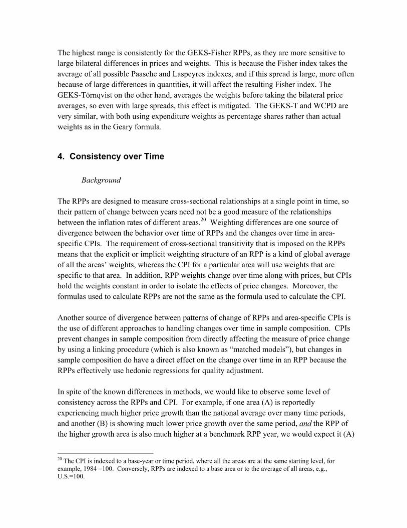
17 The new log P is given by:

*

*

log log 0.5 log log

log

a k ka kj ka jak j k

k k k

P p p pα γ

α α β φ

= +

= −

∑ ∑∑

Here log φ equals the average of the nominal per capita income for the U.S. Subscript a denotes areas 1 to 38 and subscript k denotes commodity groups 1 to 4 (Foods, Goods, Housing./Shelter Costs, Services).

The shares equation are **log log a

ia k ij ja ij a

Xw pP

α γ β⎛ ⎞

= + + ⎜ ⎟⎝ ⎠

∑

18 Deaton and Muellbauer (1980) show that the Stone P index is a good approximation of the ‘true’ P in the AI system if prices are collinear, which is frequently true of time-series prices. At the item strata level of 207 items, the correlation across areas averages around 0.6. The Stone index and the final P index for our sample differ, and it took 4 iterations for the demand model estimates to converge.

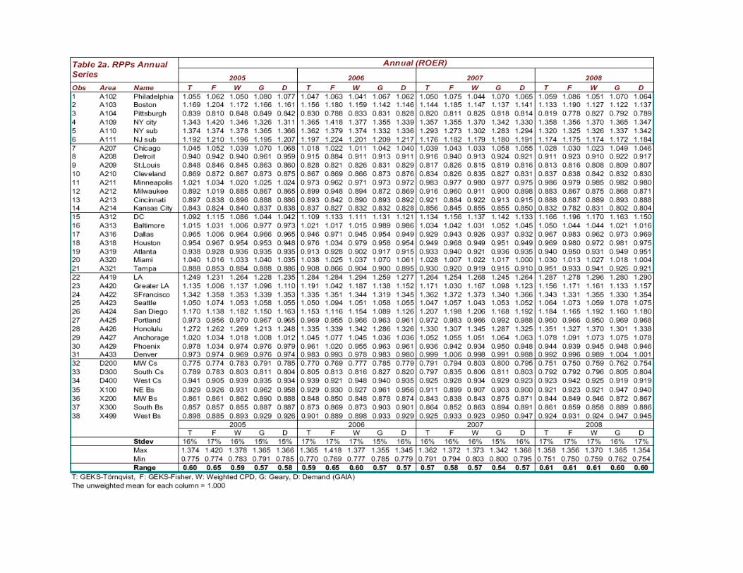
Tables B1 and B2 in the Appendix shows the estimated parameters of the constrained versions of the AI demand system for each of the estimated series (ROER, RMOC).19 There are four equations for each series, corresponding to the four groups: Food, Goods, Housing/Shelter Costs, and Services. The parameters of the fourth equation (Services) are obtained from the symmetry and homogeneity constraints of the demand system. That is, the sum of the four price parameters (γ) in each equation must sum to zero, the sum of the real expenditure per capita parameters (β) must sum to zero, and the sum of the intercepts (α) must be one. Also, the price parameters are symmetric, so that γij = γji , where i,j=1,..4. The only significant coefficients are on the Goods and Housing/Shelter equations, and for their own prices (γ2 and γ3). The Housing/Shelter coefficients (γ3) are negative for the Goods equation with a value around -0.07 for all four ROER years, and -0.12 for the RMOC multi-year series. The Housing/Shelter coefficients (γ3) are positive and significant for the Housing/Shelter equations, 0.2203 and 0.2053 for the RMOC series and between 0.1536 and 0.1144 for the ROER years. The coefficients on the per capital total expenditure variables (β) are negative for the Food equations as expected, and for most of the Housing/Shelter cost equations. The Food equations are very weak overall, while the Housing/Shelter cost equations are the strongest. The parameter estimates provides a predicted set of shares, and thus a predicted set of ‘virtual’ quantities. These virtual quantities enter into a final multilateral Geary estimation, together with the original nominal expenditures. The resulting RPPs for the 38 areas are called the GAIA RPPs. They are shown in Tables 2a (ROER) and 2b (RMOC), together with the four other traditional RPP estimates. The columns are labeled T for the GEKS-Törnqvist RPPs, F for the GEKS-Fisher, W for WCPD, G for Geary and D for the demand model in the GAIA RPPs. Looking at the summary results of these tables (the last lines labeled Standard Deviation, Maximum, Minimum and Range), there seems to be weak evidence only of a Gerschenkron effect, as the RPP range using Geary is slightly smaller than the GEKS-Törnqvist (GEKS-T) range, particularly in Table 2b.

19 The unconstrained parameter estimates are not shown, but we did calculate them. For the unconstrained estimates, we begin in the same way, with an estimate of Stone’s index, but since the demand system is linear in parameters when written in shares or budget form, it may be estimated equation by equation using OLS (ordinary least squares). As in the constrained version, the Stone index is then replaced by the new index P, and the model is re-estimated until the parameters converge and P is stable.

The highest range is consistently for the GEKS-Fisher RPPs, as they are more sensitive to large bilateral differences in prices and weights. This is because the Fisher index takes the average of all possible Paasche and Laspeyres indexes, and if this spread is large, more often because of large differences in quantities, it will affect the resulting Fisher index. The GEKS-Törnqvist on the other hand, averages the weights before taking the bilateral price averages, so even with large spreads, this effect is mitigated. The GEKS-T and WCPD are very similar, with both using expenditure weights as percentage shares rather than actual weights as in the Geary formula.

4. Consistency over Time

Background The RPPs are designed to measure cross-sectional relationships at a single point in time, so their pattern of change between years need not be a good measure of the relationships between the inflation rates of different areas.20 Weighting differences are one source of divergence between the behavior over time of RPPs and the changes over time in area-specific CPIs. The requirement of cross-sectional transitivity that is imposed on the RPPs means that the explicit or implicit weighting structure of an RPP is a kind of global average of all the areas’ weights, whereas the CPI for a particular area will use weights that are specific to that area. In addition, RPP weights change over time along with prices, but CPIs hold the weights constant in order to isolate the effects of price changes. Moreover, the formulas used to calculate RPPs are not the same as the formula used to calculate the CPI. Another source of divergence between patterns of change of RPPs and area-specific CPIs is the use of different approaches to handling changes over time in sample composition. CPIs prevent changes in sample composition from directly affecting the measure of price change by using a linking procedure (which is also known as “matched models”), but changes in sample composition do have a direct effect on the change over time in an RPP because the RPPs effectively use hedonic regressions for quality adjustment. In spite of the known differences in methods, we would like to observe some level of consistency across the RPPs and CPI. For example, if one area (A) is reportedly experiencing much higher price growth than the national average over many time periods, and another (B) is showing much lower price growth over the same period, and the RPP of the higher growth area is also much higher at a benchmark RPP year, we would expect it (A)

20 The CPI is indexed to a base-year or time period, where all the areas are at the same starting level, for example, 1984 =100. Conversely, RPPs are indexed to a base area or to the average of all areas, e.g., U.S.=100.

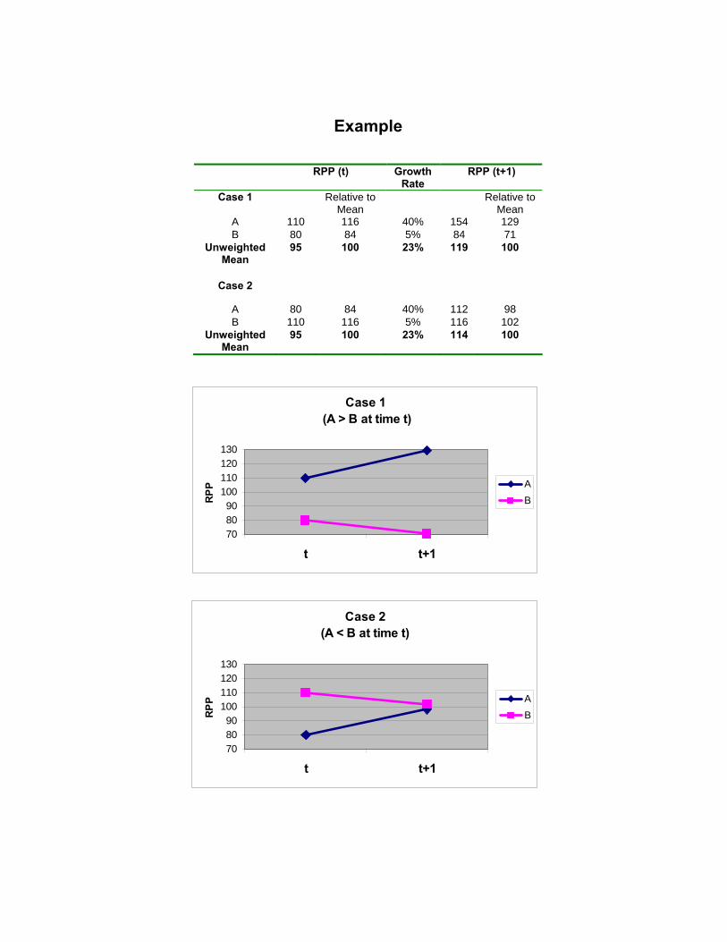
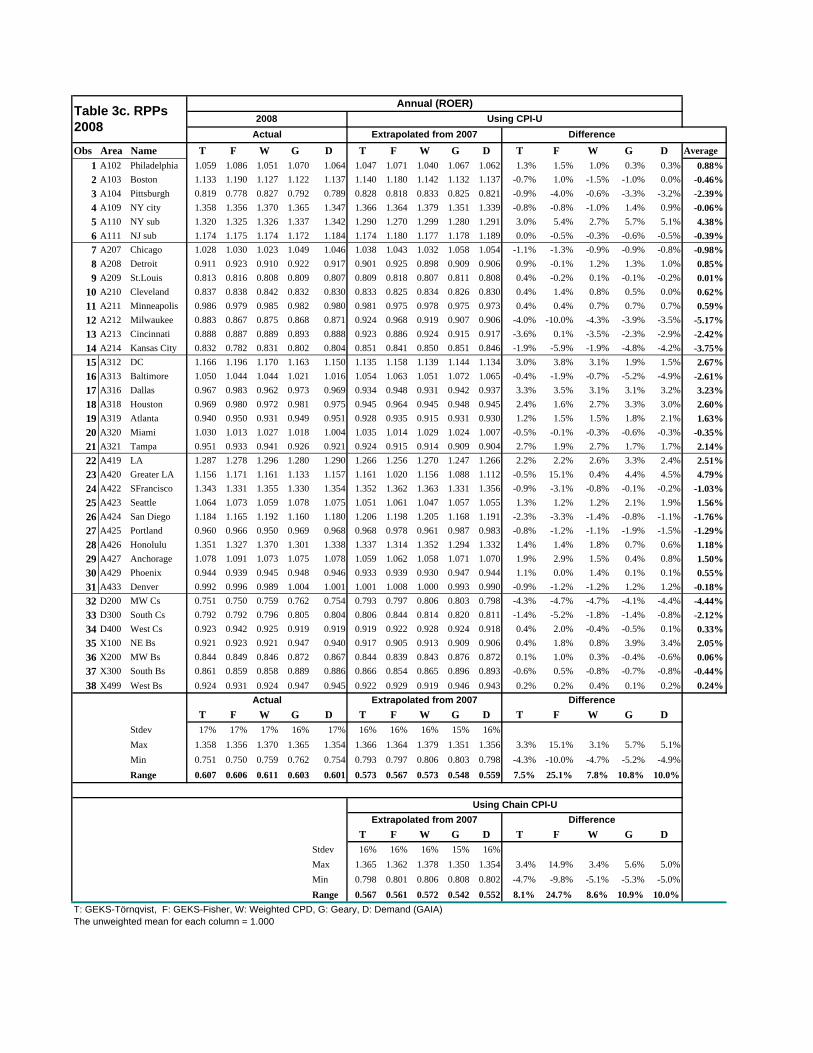
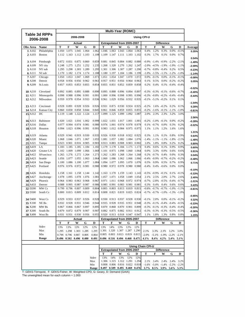
to remain higher at the next comparison year. This is illustrated in the Example (Case 1) at the end of the text. If the initial benchmark RPPs were reversed, and A was much lower than B, then even with a much higher growth rate, A will not necessarily have a higher RPP than B in the next time period. This is Case 2 in the Example. The simple example is for the unweighted case, whereas in practice, each area’s prices are weighted by its expenditures, and the CPIs and the RPPs are aggregated from more detailed level data. We use two-type of CPIs that BLS produces, the all urban CPI (CPI-U) and the chained CPI. The chained Consumer Price Index (C-CPI-U) is a Törnqvist-type index developed by the BLS in 2002 (Cage, Greenlees and Jackman, 2003). It is designed to more closely approximate a cost-of-living index than the existing fixed-weight (CPI-U) measures published by the BLS21. The former is only available at the 38 area level for research purposes, but the latter is available publicly for all areas and at detailed expenditure groupings. We are therefore able to show the detailed extrapolations using the CPI-U, but not the chained series at this time, although the results will be summarized and contrasted to the fixed-weight CPI. As described earlier, we estimated two series of RPPs because we use two housing data sources. One is the annual series from 2005-2008 using just the BLS-CPI data, and the other a multi-year rolling average for 2005-2007 and 2006-2008 using the BLS data plus the ACS rents and owner-cost data for housing from the Census Bureau. The extrapolated RPPs (2006 from 2005, 2007 from 2006 and 2008 from 2007 as well as 2006-08 from 2005-07 using the CPI-U indexes are shown in Tables 3a-3d, together with their percentage difference from the actual RPPs. Only the summary results for the Chain CPI-U are shown. The average of the differences across all five multilateral methods is also shown in the last column. The multi-year CPI used in the extrapolation for the RMOC series (Table 3d) was taken as the ratio of the unweighted geometric mean of the three years in consecutive periods (the geometric mean of the CPI indexes for 2006 through 2008 divided by the geometric mean of the CPI indexes for 2005-2007). Turning first to Table 3a, and comparing the Actual to the Extrapolated values in the summary rows, we note that the Range across methods is again highest for the F column (GEKS-Fisher), 0.650 for actual 2006 values and 0.659 for the extrapolated values using the 21 For details of the differences in construction between the two, see Table 5.1 in Cage et al (2003)

CPI-U. It drops to 0.649 when using the Chain CPI-U but is still the largest of the five methods. The GEKS-T seems to do better than the Geary or the GAIA in matching extrapolated RPPs to benchmark RPPs. Looking at the summary rows, the differences for the T (GEKS-T) columns consistently have smaller ranges than the differences for the G (Geary) or D (Demand-GAIA) columns. For Table 3a the values are 7.7% for T, 15.0% and 12.6% respectively for G and D using the CPI-U. The figures for the Chain CPI-U are very similar. In Table 3b, the range for T increases to 12.6%, then drops again to 7.5% in Table 3c. Out of the three annual ROER extrapolations, the 2007 to 2008 (Table 3c) have the smallest range, except for the F column, which is 25.1%. In contrast, the multi-year RMOC extrapolations shown in Table 3d are much closer to the actual values. The largest is still the F column (8.4%), but the others drop to 4.1%, 5.4% and 5.1% for T, G and D respectively. In addition, the volatility observed in Tables 3a-c with respect to which areas have the largest absolute differences disappears. Some of the volatility is due to the GEKS-F estimates, which are much more sensitive to outliers in the detailed data. Excluding the F column, the largest positive difference in Table 3a is for DC (G =8.6% and D=7.8%), and T=4.6% for Greater LA, and the largest negative differences are for San Diego (G=-6.4%), Detroit (D=-4.8%) and Minneapolis (T=-3.0%). In Table 3d, the largest positive differences are for DC and Anchorage (for T, G and D), and largest negative difference is for NY city (T=-2.0%) and Pittsburgh (G=-2.2%, D=-2.1%) and around -1.0% for NY city for G and D. These results strongly suggest that the multi-year series helps to reduce the effect of a) outliers in the RPPs when estimating the multilateral aggregations, and b) the variance of the housing/shelter cost estimates when using the larger RMOC series. Figures 1-5 graph the observed versus the CPI-U extrapolated values for the Multi-Year averages for each of the estimated indexes. The dashed diagonal line indicates where the extrapolated values would lie if they equaled exactly the observed values. The linear regression line and R2 are given to help compare the differences across methods. We note again that the WCPD method is very close to the GEKS-T in all situations, and in previous interarea work with this data (Aten & D’Souza 2008), we used the WCPD for our estimates. In this paper, we chose to focus on the GEKS-T and GAIA differences for two reasons. The first is that the GEKS is used extensively by international statistical offices for their comparisons, and the second that the GAIA is a demand –modified version of the Geary method, which blends the additive properties of the Geary with an economic demand system that has a theoretical appeal.

We expect the GEKS-T to be more consistent with the Chain CPI-U as they both use Törnqvist-type averages, while the Geary and the GAIA are likely to be more consistent with the fixed-weight traditional CPI-U. In the Multi-Year results, this expectation was clearly met: the GEKS-T range is smaller (3.7% versus 4.1%) when using the chain versus the fixed-weight CPI, and both the Geary and the GAIA ranges are smaller for the fixed versus chain extrapolation differences (5.4% Geary fixed CPI, 5.6% Geary chain and 5.1% GAIA fixed versus 5.3% GAIA chain). In the Annual series, the same expectations are met for the 2006 and 2008 extrapolations, but for the 2007 series, all three methods have smaller ranges using the chain series. We saw above that 2007 also has the greatest variability between actual and extrapolated values, particularly for the New York suburbs and San Diego areas, and further work is needed to pinpoint the reasons for this greater variability in the ROER results. Thirty-four out of the thirty-eight areas (90%) have differences of less than 2.0% in the Multi-Year estimates using the GEKS-T. In contrast, for 2006 and 2008, only twenty-eight (74%) have differences less than 2.0%, and even fewer, twenty-one (55%) in 2007. The pattern is repeated across methods, and underscores the greater stability and consistency of the multi-year series with respect to the CPI.

5. Conclusion We know from the international comparison literature that it is difficult to achieve space-time consistency when looking at national growth rates versus benchmark year price level differences. One reason is that the growth rates are measured by own-country statistical agencies using varying methods and practices, while benchmark comparisons of price levels are done by regional and international agencies seeking to match different goods and services across countries.22 Furthermore, to adjust for quality change when items exit or enter the sample, indexes aimed at measuring price change over time rely mainly on “matched models” or “linking”, a procedure that effectively assumes that price level differences between items are measures of the value of their quality differences. The hedonic regression procedures that are mainly used to control for quality differentials in indexes aimed at measuring price change over space do not make this assumption. Finally, Feenstra et al. (2009, p.172) and Rao et al (2008, note 8, p.190) note that homotheticity usually fails to hold in national consumption data, but without homotheticity “… when the

22 See the ICP by the World Bank (www.worldbank.org/data/icp). The SNA (System of National Accounts) seeks to minimize methodological differences across countries, but methods and practices still vary, particularly for difficult to measure items, such as services and housing costs

NPC (National Price Comparison) is done in one benchmark year and then extrapolated forward using the NPC (in the previous year) there is no reason to expect that we will obtain a result that matches the NPC done in that future year.” Nevertheless, the demand system coefficient estimates used in our GAIA model results imply that non-homotheticity is a trivial factor in these types of discrepancies in the case of regions of the US. In the U.S., we expect the differences across areas to be less than what one finds across countries. We also have the advantage of working with the same price and expenditure data that enter the estimation of the Consumer Price Index, enabling more detailed and comprehensive comparisons of similar goods and services. We estimated four traditional multilateral price indexes or RPPs, and one economic framework RPP, the GAIA (Neary, 2004). For each method, we used two sources of data for the housing cost component. The first was from the CPI, called ROER (for Rents and Owners’ Equivalent Rents), while the second was from the microdata of the American Community Survey of the Census Bureau, labeled RMOC (for Rents and Monthly Owners’ Costs). The RMOC has better geographic coverage, including rural areas that are not in the CPI. For the remaining items (207 non-housing items), we use the annual price and expenditure data from the CPI. We then compared the values of the RPPs extrapolated forward using area-specific CPIs to the subsequent actual ‘benchmark’ RPP. This is equivalent to the NPC approach in Feenstra et al (2009). The extrapolations used two kinds of CPI series. One is the published CPI-U (Urban consumers), which is publicly available at the 38 area level detail, and the other is the new Chain CPI-U, which has not been released at the area level.23 We expected the extrapolated GEKS-Törnqvist RPPs to be closer to the Chain CPI-U, and the GAIA, and to a lesser extent the Geary RPPs, to be closer to the Laspeyres type CPI-U. We also expected the RPPs calculated using the multi-year housing data (ROMC) to be more robust than the annual ROER series. These expectations were met, although the difference between the Geary and the GAIA estimates were smaller than expected when comparing consistency over time. This could be due to a) the lack of a strong Gerschenkron effect that is more prevalent when comparing very dissimilar geographic areas, and b) to the fact that by construction, the GAIA estimates new ‘virtual’ quantity shares which adjust to the expected demand in each period. Thus, the Laspeyres CPI-U would be more similar to the Geary fixed weight extrapolation than the GAIA. The objective of this work is ultimately to adjust regional incomes at the state and more detailed metropolitan level than the 38 areas reported here. However, we are limited by the 23 See Cage et al (2003) for details.

price and expenditure data collected by the BLS, as their sampling framework was designed for measures over time, not across space. It is also for this reason that the ROER data is relatively sparse when compared to the RMOC from the Census Bureau, so we compare the two as a way to reduce the variability over time of the RPPs, since housing costs are a large component of the expenditures and the price variation in the surveys. We find that using a multi-year rolling average for the housing component results in RPPs whose changes are generally consistent with the CPIs over the period studied (2005-2008). Only three out of the 38 areas (New York City, Washington DC and Anchorage AK) had differences greater than 2.0% between actual and extrapolated versions using the multi-year average and 30 out of 38 have differences of less than 1%. By the end of 2010, the Census Bureau is expected to release their five-year (2005-2009) multi-year average for the American Community Survey, and we will update our results, hoping for even more robust estimates. In the interim, we will investigate ways to extend the geographic coverage of the RPPs, thereby allowing us to obtain a measure that can be used to adjust BEA’s personal income estimates at the state and detailed metropolitan area levels.

TABLES and CHARTS

Table 1a. Geary National Average Price Levels (πs)

Obs Group 2005 2006 2007 2008 2005-2007 2006-2008

ROER* RMOC**

1 Food 1.0085 1.0031 1.0041 1.0079 1.0042 1.00422 Goods 1.0150 1.0141 1.0146 1.0150 1.0122 1.01263 Housing costs

ROER/RMOC 0.9812 0.9841 0.9831 0.9832 0.9859 0.98624 Services 1.0025 1.0021 1.0025 1.0010 1.0017 1.0012

* ROER: Rents and Owners’ Equivalent Rents from BLS CPI, annual series; **RMOC: Rents and Monthly Owner Costs from ACS Housing survey, 3-year average

Table 1b. GAIA National Average Price Levels (πs)

Obs Group 2005 2006 2007 2008 2005-2007 2006-2008

ROER* RMOC**

1 Food 1.0081 1.0040 1.0066 1.0099 1.0071 1.00402 Goods 1.0057 1.0145 1.0086 1.0149 1.0039 1.00483 Housing costs

ROER/RMOC 0.9992 0.9961 0.9933 0.9885 0.9992 0.99574 Services 0.9981 0.9984 1.0052 1.0016 0.9975 1.0016

* ROER: Rents and Owners’ Equivalent Rents from BLS CPI, annual series; **RMOC: Rents and Monthly Owner Costs from ACS Housing survey, 3-year average

Example

RPP (t) Growth Rate

RPP (t+1)

Case 1 Relative to Mean

Relative to Mean

A 110 116 40% 154 129 B 80 84 5% 84 71

Unweighted Mean

95 100 23% 119 100

Case 2

A 80 84 40% 112 98 B 110 116 5% 116 102

Unweighted Mean

95 100 23% 114 100

Case 1 (A > B at time t)

708090

100110120130

t t+1

RPP A

B

Case 2(A < B at time t)

708090

100110120130

t t+1

RP

P AB

Chart 1. Price Parities U.S. Average and Selected Areas: 2005

Figure 1. GEKS-Tornqvist

Multi-Year GEKS-Tornqvist

y = 1.0005x - 7E-05R2 = 0.996

0.70

0.80

0.90

1.00

1.10

1.20

1.30

1.40

0.70 0.80 0.90 1.00 1.10 1.20 1.30 1.40

Actual 2006-2008

Extr

apol

ated

from

200

5-20

07

0.9

0.95

1

1.05

1.1

Food Goods Rents Services

Denver

Portland

US PRICES(Geary)Minneapolis

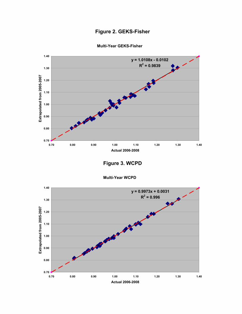
Figure 2. GEKS-Fisher

Figure 3. WCPD

Multi-Year GEKS-Fisher

y = 1.0108x - 0.0102R2 = 0.9839

0.70

0.80

0.90

1.00

1.10

1.20

1.30

1.40

0.70 0.80 0.90 1.00 1.10 1.20 1.30 1.40

Actual 2006-2008

Extr

apol

ated

from

200

5-20

07

Multi-Year WCPD

y = 0.9973x + 0.0031R2 = 0.996

0.70

0.80

0.90

1.00

1.10

1.20

1.30

1.40

0.70 0.80 0.90 1.00 1.10 1.20 1.30 1.40

Actual 2006-2008

Extr

apol

ated

from

200

5-20

07

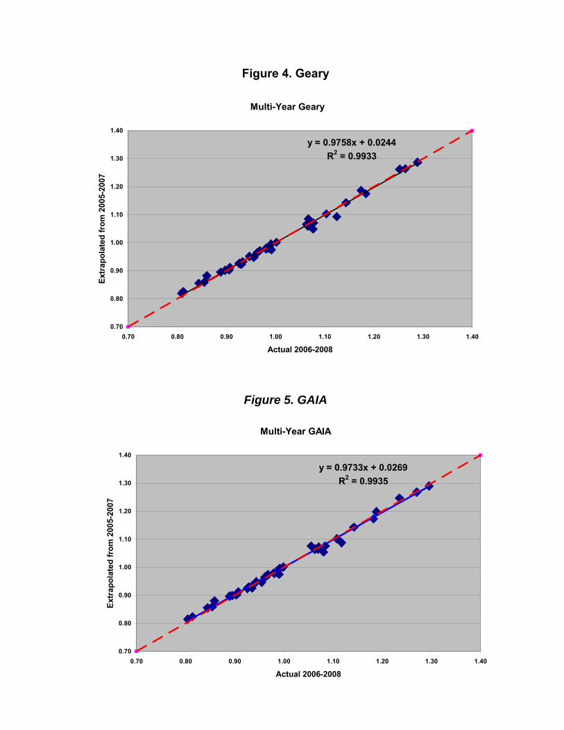
Figure 4. Geary

Figure 5. GAIA

Multi-Year Geary

y = 0.9758x + 0.0244R2 = 0.9933

0.70

0.80

0.90

1.00

1.10

1.20

1.30

1.40

0.70 0.80 0.90 1.00 1.10 1.20 1.30 1.40

Actual 2006-2008

Extr

apol

ated

from

200

5-20

07

Multi-Year GAIA

y = 0.9733x + 0.0269R2 = 0.9935

0.70

0.80

0.90

1.00

1.10

1.20

1.30

1.40

0.70 0.80 0.90 1.00 1.10 1.20 1.30 1.40

Actual 2006-2008

Extr

apol

ated

from

200

5-20

07

Obs Area Name T F W G D T F W G D T F W G D Average1 A102 Philadelphia 1.047 1.063 1.041 1.067 1.062 1.061 1.068 1.056 1.086 1.083 -1.4% -0.5% -1.5% -1.9% -2.0% -1.48%2 A103 Boston 1.156 1.180 1.159 1.142 1.146 1.168 1.202 1.171 1.165 1.160 -1.1% -2.2% -1.2% -2.3% -1.4% -1.63%3 A104 Pittsburgh 0.830 0.788 0.833 0.831 0.828 0.839 0.809 0.847 0.848 0.841 -0.9% -2.1% -1.4% -1.6% -1.3% -1.45%4 A109 NY city 1.365 1.418 1.377 1.355 1.339 1.351 1.428 1.354 1.334 1.318 1.4% -1.0% 2.3% 2.1% 2.1% 1.39%5 A110 NY sub 1.362 1.379 1.374 1.332 1.336 1.368 1.368 1.372 1.360 1.361 -0.6% 1.2% 0.2% -2.8% -2.4% -0.89%6 A111 NJ sub 1.197 1.224 1.201 1.209 1.217 1.210 1.229 1.214 1.213 1.225 -1.3% -0.4% -1.3% -0.5% -0.8% -0.85%7 A207 Chicago 1.018 1.022 1.011 1.042 1.040 1.033 1.040 1.027 1.058 1.056 -1.6% -1.7% -1.6% -1.5% -1.6% -1.60%8 A208 Detroit 0.915 0.884 0.911 0.913 0.911 0.939 0.942 0.940 0.961 0.959 -2.4% -5.8% -2.9% -4.8% -4.8% -4.13%9 A209 St.Louis 0.828 0.821 0.826 0.831 0.829 0.837 0.834 0.833 0.851 0.849 -0.9% -1.4% -0.7% -2.0% -1.9% -1.37%

10 A210 Cleveland 0.867 0.869 0.866 0.873 0.876 0.857 0.860 0.855 0.860 0.863 1.0% 0.9% 1.2% 1.3% 1.4% 1.14%11 A211 Minneapolis 0.973 0.962 0.971 0.973 0.972 1.003 1.016 1.003 1.007 1.007 -3.0% -5.4% -3.2% -3.5% -3.5% -3.72%12 A212 Milwaukee 0.899 0.948 0.894 0.872 0.869 0.885 1.011 0.877 0.860 0.858 1.5% -6.3% 1.6% 1.2% 1.1% -0.18%13 A213 Cincinnati 0.893 0.842 0.890 0.893 0.892 0.902 0.843 0.902 0.894 0.891 -0.9% -0.1% -1.2% 0.0% 0.0% -0.44%14 A214 Kansas City 0.837 0.827 0.832 0.832 0.828 0.838 0.819 0.835 0.832 0.833 -0.1% 0.8% -0.2% 0.1% -0.5% 0.01%15 A312 DC 1.109 1.133 1.111 1.131 1.121 1.093 1.117 1.087 1.046 1.043 1.6% 1.6% 2.4% 8.6% 7.8% 4.40%16 A313 Baltimore 1.021 1.017 1.015 0.989 0.986 1.027 1.043 1.019 0.989 0.985 -0.7% -2.6% -0.3% 0.1% 0.1% -0.68%17 A316 Dallas 0.946 0.971 0.945 0.954 0.949 0.963 1.004 0.962 0.964 0.963 -1.7% -3.3% -1.7% -1.0% -1.4% -1.81%18 A318 Houston 0.976 1.034 0.979 0.958 0.954 0.950 0.962 0.950 0.948 0.944 2.6% 7.2% 2.9% 1.0% 1.0% 2.93%19 A319 Atlanta 0.913 0.928 0.902 0.917 0.915 0.932 0.922 0.930 0.929 0.930 -2.0% 0.6% -2.9% -1.2% -1.5% -1.39%20 A320 Miami 1.038 1.025 1.037 1.070 1.061 1.058 1.033 1.050 1.057 1.052 -2.0% -0.9% -1.3% 1.3% 0.8% -0.39%21 A321 Tampa 0.908 0.866 0.904 0.900 0.895 0.896 0.860 0.891 0.895 0.893 1.2% 0.6% 1.3% 0.5% 0.2% 0.77%22 A419 LA 1.284 1.284 1.294 1.259 1.277 1.262 1.243 1.276 1.240 1.247 2.3% 4.1% 1.8% 1.8% 3.0% 2.59%23 A420 Greater LA 1.191 1.042 1.187 1.138 1.152 1.145 1.015 1.147 1.106 1.121 4.6% 2.7% 3.9% 3.2% 3.1% 3.51%24 A422 SFrancisco 1.335 1.351 1.344 1.319 1.345 1.342 1.358 1.353 1.339 1.353 -0.8% -0.7% -0.9% -2.0% -0.7% -1.02%25 A423 Seattle 1.050 1.094 1.051 1.058 1.055 1.054 1.078 1.057 1.063 1.060 -0.4% 1.6% -0.6% -0.4% -0.5% -0.06%26 A424 San Diego 1.153 1.116 1.154 1.089 1.126 1.173 1.140 1.185 1.153 1.165 -2.0% -2.5% -3.1% -6.4% -4.0% -3.60%27 A425 Portland 0.969 0.955 0.966 0.963 0.961 0.967 0.951 0.964 0.961 0.960 0.1% 0.4% 0.1% 0.2% 0.1% 0.19%28 A426 Honolulu 1.335 1.339 1.342 1.286 1.326 1.305 1.295 1.303 1.244 1.280 3.0% 4.4% 3.9% 4.2% 4.6% 4.03%29 A427 Anchorage 1.045 1.077 1.045 1.036 1.036 1.019 1.033 1.017 1.006 1.011 2.6% 4.4% 2.8% 3.0% 2.5% 3.05%30 A429 Phoenix 0.961 1.020 0.955 0.963 0.961 0.976 1.032 0.971 0.973 0.977 -1.5% -1.2% -1.7% -1.0% -1.6% -1.39%31 A433 Denver 0.983 0.993 0.978 0.983 0.980 0.977 0.977 0.973 0.980 0.978 0.6% 1.5% 0.5% 0.3% 0.2% 0.64%32 D200 MW Cs 0.770 0.769 0.777 0.785 0.779 0.771 0.770 0.780 0.787 0.781 0.0% -0.1% -0.2% -0.2% -0.2% -0.17%33 D300 South Cs 0.805 0.813 0.816 0.827 0.820 0.795 0.788 0.809 0.817 0.810 1.1% 2.5% 0.7% 1.0% 1.0% 1.27%34 D400 West Cs 0.939 0.921 0.948 0.940 0.935 0.941 0.905 0.938 0.935 0.934 -0.1% 1.6% 1.0% 0.6% 0.1% 0.63%35 X100 NE Bs 0.929 0.930 0.927 0.961 0.956 0.932 0.929 0.935 0.965 0.961 -0.4% 0.0% -0.8% -0.4% -0.5% -0.39%36 X200 MW Bs 0.848 0.850 0.848 0.878 0.874 0.855 0.855 0.855 0.883 0.881 -0.7% -0.5% -0.7% -0.5% -0.7% -0.59%37 X300 South Bs 0.873 0.869 0.873 0.903 0.901 0.857 0.857 0.855 0.887 0.887 1.6% 1.2% 1.8% 1.7% 1.4% 1.53%38 X499 West Bs 0.901 0.889 0.898 0.933 0.929 0.894 0.881 0.889 0.925 0.922 0.7% 0.8% 0.9% 0.8% 0.6% 0.77%

T F W G D T F W G D T F W G DStdev 17% 17% 17% 15% 16% 16% 17% 16% 15% 16%Max 1.365 1.418 1.377 1.355 1.345 1.368 1.428 1.372 1.360 1.361 4.6% 7.2% 3.9% 8.6% 7.8%Min 0.770 0.769 0.777 0.785 0.779 0.771 0.770 0.780 0.787 0.781 -3.0% -6.3% -3.2% -6.4% -4.8%Range 0.595 0.650 0.600 0.570 0.566 0.597 0.659 0.592 0.573 0.579 7.7% 13.5% 7.2% 15.0% 12.6%

T F W G D T F W G DStdev 16% 17% 16% 15% 16%

Max 1.377 1.420 1.381 1.369 1.370 4.9% 7.3% 4.2% 8.4% 7.7%Min 0.772 0.771 0.781 0.788 0.782 -2.7% -6.6% -3.3% -6.7% -4.9%Range 0.605 0.649 0.601 0.581 0.587 7.6% 13.9% 7.5% 15.1% 12.6%

Table 3a. RPPs 2006

T: GEKS-Törnqvist, F: GEKS-Fisher, W: Weighted CPD, G: Geary, D: Demand (GAIA)The unweighted mean for each column = 1.000

Actual

Extrapolated from 2005

Using Chain CPI-U

Difference

Annual (ROER)2006 Using CPI-U

Extrapolated from 2005 Difference

Extrapolated from 2005 Difference

Actual

Obs Area Name T F W G D T F W G D T F W G D Average1 A102 Philadelphia 1.050 1.075 1.044 1.070 1.065 1.041 1.057 1.034 1.061 1.056 1.0% 1.8% 1.0% 1.0% 0.9% 1.12%2 A103 Boston 1.144 1.185 1.147 1.137 1.141 1.146 1.170 1.149 1.132 1.137 -0.2% 1.5% -0.2% 0.4% 0.5% 0.40%3 A104 Pittsburgh 0.820 0.811 0.825 0.818 0.814 0.831 0.789 0.834 0.832 0.829 -1.1% 2.2% -0.9% -1.5% -1.5% -0.56%4 A109 NY city 1.357 1.355 1.370 1.342 1.330 1.377 1.430 1.389 1.367 1.351 -1.9% -7.5% -1.9% -2.4% -2.1% -3.17%5 A110 NY sub 1.293 1.273 1.302 1.283 1.294 1.358 1.375 1.369 1.328 1.332 -6.5% -10.2% -6.8% -4.5% -3.9% -6.37%6 A111 NJ sub 1.176 1.182 1.179 1.180 1.191 1.192 1.219 1.196 1.204 1.212 -1.6% -3.8% -1.7% -2.4% -2.1% -2.32%7 A207 Chicago 1.039 1.043 1.033 1.058 1.055 1.022 1.027 1.015 1.047 1.044 1.7% 1.7% 1.8% 1.2% 1.1% 1.48%8 A208 Detroit 0.916 0.940 0.913 0.924 0.921 0.906 0.876 0.902 0.905 0.902 1.0% 6.4% 1.0% 1.9% 1.9% 2.43%9 A209 St.Louis 0.817 0.826 0.815 0.819 0.816 0.822 0.814 0.820 0.825 0.823 -0.5% 1.1% -0.5% -0.6% -0.7% -0.22%

10 A210 Cleveland 0.834 0.826 0.835 0.827 0.831 0.862 0.864 0.862 0.868 0.872 -2.8% -3.8% -2.6% -4.1% -4.1% -3.49%11 A211 Minneapolis 0.983 0.977 0.980 0.977 0.975 0.972 0.961 0.969 0.971 0.970 1.2% 1.6% 1.1% 0.6% 0.4% 0.98%12 A212 Milwaukee 0.916 0.960 0.911 0.900 0.898 0.893 0.942 0.888 0.866 0.864 2.3% 1.8% 2.3% 3.4% 3.5% 2.66%13 A213 Cincinnati 0.921 0.884 0.922 0.913 0.915 0.892 0.840 0.888 0.892 0.890 2.9% 4.3% 3.4% 2.1% 2.5% 3.05%14 A214 Kansas City 0.856 0.845 0.855 0.855 0.850 0.835 0.825 0.830 0.830 0.826 2.1% 2.0% 2.5% 2.5% 2.5% 2.32%15 A312 DC 1.134 1.156 1.137 1.142 1.133 1.114 1.137 1.115 1.136 1.126 2.0% 1.9% 2.2% 0.6% 0.7% 1.49%16 A313 Baltimore 1.034 1.042 1.031 1.052 1.045 1.033 1.030 1.028 1.002 0.998 0.0% 1.3% 0.4% 5.0% 4.7% 2.27%17 A316 Dallas 0.929 0.943 0.926 0.937 0.932 0.934 0.959 0.934 0.942 0.937 -0.5% -1.6% -0.7% -0.5% -0.5% -0.78%18 A318 Houston 0.949 0.968 0.949 0.951 0.949 0.965 1.023 0.968 0.948 0.944 -1.7% -5.5% -1.9% 0.4% 0.5% -1.65%19 A319 Atlanta 0.933 0.940 0.921 0.936 0.935 0.916 0.931 0.905 0.921 0.918 1.7% 0.9% 1.5% 1.5% 1.7% 1.47%20 A320 Miami 1.028 1.007 1.022 1.017 1.000 1.051 1.038 1.051 1.084 1.074 -2.3% -3.1% -2.9% -6.7% -7.4% -4.49%21 A321 Tampa 0.930 0.920 0.919 0.915 0.910 0.928 0.885 0.924 0.920 0.915 0.2% 3.5% -0.4% -0.5% -0.5% 0.45%22 A419 LA 1.264 1.254 1.268 1.245 1.264 1.289 1.288 1.299 1.263 1.282 -2.5% -3.4% -3.0% -1.8% -1.8% -2.50%23 A420 Greater LA 1.171 1.030 1.167 1.098 1.123 1.197 1.047 1.193 1.143 1.157 -2.6% -1.8% -2.6% -4.5% -3.5% -2.98%24 A422 SFrancisco 1.362 1.372 1.373 1.340 1.366 1.340 1.356 1.349 1.324 1.350 2.3% 1.6% 2.4% 1.6% 1.6% 1.89%25 A423 Seattle 1.047 1.057 1.043 1.053 1.052 1.061 1.106 1.062 1.070 1.067 -1.4% -4.9% -1.9% -1.6% -1.5% -2.27%26 A424 San Diego 1.207 1.198 1.206 1.168 1.192 1.146 1.109 1.147 1.082 1.119 6.1% 8.9% 5.9% 8.6% 7.3% 7.33%27 A425 Portland 0.972 0.983 0.966 0.992 0.988 0.976 0.962 0.973 0.971 0.968 -0.4% 2.0% -0.7% 2.1% 2.0% 1.00%28 A426 Honolulu 1.330 1.307 1.345 1.287 1.325 1.359 1.364 1.366 1.309 1.350 -2.9% -5.7% -2.1% -2.2% -2.5% -3.09%29 A427 Anchorage 1.052 1.055 1.051 1.064 1.063 1.038 1.070 1.038 1.029 1.029 1.3% -1.5% 1.3% 3.5% 3.4% 1.60%30 A429 Phoenix 0.936 0.942 0.934 0.950 0.948 0.965 1.025 0.959 0.968 0.965 -2.9% -8.3% -2.6% -1.8% -1.7% -3.46%31 A433 Denver 0.999 1.006 0.998 0.991 0.988 0.976 0.986 0.972 0.976 0.974 2.4% 2.0% 2.7% 1.4% 1.4% 1.97%32 D200 MW Cs 0.791 0.794 0.803 0.800 0.795 0.770 0.769 0.777 0.785 0.779 2.0% 2.5% 2.6% 1.5% 1.6% 2.05%33 D300 South Cs 0.797 0.835 0.806 0.811 0.803 0.803 0.811 0.814 0.825 0.817 -0.6% 2.4% -0.8% -1.4% -1.4% -0.36%34 D400 West Cs 0.925 0.928 0.934 0.929 0.923 0.945 0.926 0.954 0.945 0.940 -2.0% 0.2% -2.0% -1.7% -1.8% -1.45%35 X100 NE Bs 0.911 0.899 0.907 0.903 0.900 0.926 0.927 0.924 0.959 0.953 -1.5% -2.8% -1.7% -5.6% -5.3% -3.39%36 X200 MW Bs 0.843 0.838 0.843 0.875 0.871 0.847 0.849 0.847 0.878 0.874 -0.4% -1.1% -0.5% -0.3% -0.2% -0.52%37 X300 South Bs 0.864 0.852 0.863 0.894 0.891 0.873 0.869 0.873 0.903 0.901 -0.9% -1.7% -1.0% -0.9% -1.0% -1.10%38 X499 West Bs 0.925 0.933 0.923 0.950 0.947 0.902 0.890 0.899 0.934 0.930 2.3% 4.3% 2.5% 1.6% 1.7% 2.48%


T F W G D T F W G DStdev 16% 17% 16% 15% 16%Max 1.372 1.426 1.384 1.363 1.350 5.6% 8.5% 5.4% 8.2% 6.9%Min 0.773 0.771 0.780 0.788 0.782 -6.8% -10.5% -7.0% -6.6% -7.3%Range 0.599 0.654 0.605 0.575 0.568 12.4% 19.0% 12.4% 14.8% 14.1%

Table 3b. RPPs 2007


Actual Extrapolated from 2006 Difference2007 Using CPI-U

Annual (ROER)

Difference

Extrapolated from 2006 DifferenceUsing Chain CPI-U

Actual Extrapolated from 2006

Obs Area Name T F W G D T F W G D T F W G D Average1 A102 Philadelphia 1.059 1.086 1.051 1.070 1.064 1.047 1.071 1.040 1.067 1.062 1.3% 1.5% 1.0% 0.3% 0.3% 0.88%2 A103 Boston 1.133 1.190 1.127 1.122 1.137 1.140 1.180 1.142 1.132 1.137 -0.7% 1.0% -1.5% -1.0% 0.0% -0.46%3 A104 Pittsburgh 0.819 0.778 0.827 0.792 0.789 0.828 0.818 0.833 0.825 0.821 -0.9% -4.0% -0.6% -3.3% -3.2% -2.39%4 A109 NY city 1.358 1.356 1.370 1.365 1.347 1.366 1.364 1.379 1.351 1.339 -0.8% -0.8% -1.0% 1.4% 0.9% -0.06%5 A110 NY sub 1.320 1.325 1.326 1.337 1.342 1.290 1.270 1.299 1.280 1.291 3.0% 5.4% 2.7% 5.7% 5.1% 4.38%6 A111 NJ sub 1.174 1.175 1.174 1.172 1.184 1.174 1.180 1.177 1.178 1.189 0.0% -0.5% -0.3% -0.6% -0.5% -0.39%7 A207 Chicago 1.028 1.030 1.023 1.049 1.046 1.038 1.043 1.032 1.058 1.054 -1.1% -1.3% -0.9% -0.9% -0.8% -0.98%8 A208 Detroit 0.911 0.923 0.910 0.922 0.917 0.901 0.925 0.898 0.909 0.906 0.9% -0.1% 1.2% 1.3% 1.0% 0.85%9 A209 St.Louis 0.813 0.816 0.808 0.809 0.807 0.809 0.818 0.807 0.811 0.808 0.4% -0.2% 0.1% -0.1% -0.2% 0.01%

10 A210 Cleveland 0.837 0.838 0.842 0.832 0.830 0.833 0.825 0.834 0.826 0.830 0.4% 1.4% 0.8% 0.5% 0.0% 0.62%11 A211 Minneapolis 0.986 0.979 0.985 0.982 0.980 0.981 0.975 0.978 0.975 0.973 0.4% 0.4% 0.7% 0.7% 0.7% 0.59%12 A212 Milwaukee 0.883 0.867 0.875 0.868 0.871 0.924 0.968 0.919 0.907 0.906 -4.0% -10.0% -4.3% -3.9% -3.5% -5.17%13 A213 Cincinnati 0.888 0.887 0.889 0.893 0.888 0.923 0.886 0.924 0.915 0.917 -3.6% 0.1% -3.5% -2.3% -2.9% -2.42%14 A214 Kansas City 0.832 0.782 0.831 0.802 0.804 0.851 0.841 0.850 0.851 0.846 -1.9% -5.9% -1.9% -4.8% -4.2% -3.75%15 A312 DC 1.166 1.196 1.170 1.163 1.150 1.135 1.158 1.139 1.144 1.134 3.0% 3.8% 3.1% 1.9% 1.5% 2.67%16 A313 Baltimore 1.050 1.044 1.044 1.021 1.016 1.054 1.063 1.051 1.072 1.065 -0.4% -1.9% -0.7% -5.2% -4.9% -2.61%17 A316 Dallas 0.967 0.983 0.962 0.973 0.969 0.934 0.948 0.931 0.942 0.937 3.3% 3.5% 3.1% 3.1% 3.2% 3.23%18 A318 Houston 0.969 0.980 0.972 0.981 0.975 0.945 0.964 0.945 0.948 0.945 2.4% 1.6% 2.7% 3.3% 3.0% 2.60%19 A319 Atlanta 0.940 0.950 0.931 0.949 0.951 0.928 0.935 0.915 0.931 0.930 1.2% 1.5% 1.5% 1.8% 2.1% 1.63%20 A320 Miami 1.030 1.013 1.027 1.018 1.004 1.035 1.014 1.029 1.024 1.007 -0.5% -0.1% -0.3% -0.6% -0.3% -0.35%21 A321 Tampa 0.951 0.933 0.941 0.926 0.921 0.924 0.915 0.914 0.909 0.904 2.7% 1.9% 2.7% 1.7% 1.7% 2.14%22 A419 LA 1.287 1.278 1.296 1.280 1.290 1.266 1.256 1.270 1.247 1.266 2.2% 2.2% 2.6% 3.3% 2.4% 2.51%23 A420 Greater LA 1.156 1.171 1.161 1.133 1.157 1.161 1.020 1.156 1.088 1.112 -0.5% 15.1% 0.4% 4.4% 4.5% 4.79%24 A422 SFrancisco 1.343 1.331 1.355 1.330 1.354 1.352 1.362 1.363 1.331 1.356 -0.9% -3.1% -0.8% -0.1% -0.2% -1.03%25 A423 Seattle 1.064 1.073 1.059 1.078 1.075 1.051 1.061 1.047 1.057 1.055 1.3% 1.2% 1.2% 2.1% 1.9% 1.56%26 A424 San Diego 1.184 1.165 1.192 1.160 1.180 1.206 1.198 1.205 1.168 1.191 -2.3% -3.3% -1.4% -0.8% -1.1% -1.76%27 A425 Portland 0.960 0.966 0.950 0.969 0.968 0.968 0.978 0.961 0.987 0.983 -0.8% -1.2% -1.1% -1.9% -1.5% -1.29%28 A426 Honolulu 1.351 1.327 1.370 1.301 1.338 1.337 1.314 1.352 1.294 1.332 1.4% 1.4% 1.8% 0.7% 0.6% 1.18%29 A427 Anchorage 1.078 1.091 1.073 1.075 1.078 1.059 1.062 1.058 1.071 1.070 1.9% 2.9% 1.5% 0.4% 0.8% 1.50%30 A429 Phoenix 0.944 0.939 0.945 0.948 0.946 0.933 0.939 0.930 0.947 0.944 1.1% 0.0% 1.4% 0.1% 0.1% 0.55%31 A433 Denver 0.992 0.996 0.989 1.004 1.001 1.001 1.008 1.000 0.993 0.990 -0.9% -1.2% -1.2% 1.2% 1.2% -0.18%32 D200 MW Cs 0.751 0.750 0.759 0.762 0.754 0.793 0.797 0.806 0.803 0.798 -4.3% -4.7% -4.7% -4.1% -4.4% -4.44%33 D300 South Cs 0.792 0.792 0.796 0.805 0.804 0.806 0.844 0.814 0.820 0.811 -1.4% -5.2% -1.8% -1.4% -0.8% -2.12%34 D400 West Cs 0.923 0.942 0.925 0.919 0.919 0.919 0.922 0.928 0.924 0.918 0.4% 2.0% -0.4% -0.5% 0.1% 0.33%35 X100 NE Bs 0.921 0.923 0.921 0.947 0.940 0.917 0.905 0.913 0.909 0.906 0.4% 1.8% 0.8% 3.9% 3.4% 2.05%36 X200 MW Bs 0.844 0.849 0.846 0.872 0.867 0.844 0.839 0.843 0.876 0.872 0.1% 1.0% 0.3% -0.4% -0.6% 0.06%37 X300 South Bs 0.861 0.859 0.858 0.889 0.886 0.866 0.854 0.865 0.896 0.893 -0.6% 0.5% -0.8% -0.7% -0.8% -0.44%38 X499 West Bs 0.924 0.931 0.924 0.947 0.945 0.922 0.929 0.919 0.946 0.943 0.2% 0.2% 0.4% 0.1% 0.2% 0.24%




Table 3c. RPPs 2008 Actual Extrapolated from 2007

2008 Using CPI-U

Extrapolated from 2007 DifferenceActual

Extrapolated from 2007 DifferenceUsing Chain CPI-U

Difference

Annual (ROER)

Obs Area Name T F W G D T F W G D T F W G D Average1 A102 Philadelphia 1.050 1.075 1.045 1.064 1.062 1.046 1.063 1.043 1.064 1.063 0.4% 1.2% 0.3% 0.0% -0.1% 0.35%2 A103 Boston 1.112 1.163 1.112 1.103 1.108 1.109 1.147 1.111 1.103 1.102 0.3% 1.7% 0.1% 0.0% 0.7%

0.54%3 A104 Pittsburgh 0.872 0.831 0.875 0.860 0.859 0.881 0.845 0.884 0.882 0.880 -0.9% -1.4% -0.9% -2.2% -2.1% -1.49%4 A109 NY city 1.248 1.275 1.251 1.252 1.235 1.268 1.320 1.270 1.262 1.247 -2.0% -4.5% -1.9% -1.0% -1.1% -2.09%5 A110 NY sub 1.295 1.298 1.303 1.289 1.295 1.301 1.306 1.307 1.287 1.290 -0.7% -0.8% -0.4% 0.2% 0.5% -0.23%6 A111 NJ sub 1.170 1.182 1.174 1.174 1.188 1.180 1.197 1.184 1.186 1.199 -1.0% -1.5% -1.1% -1.2% -1.0% -1.14%7 A207 Chicago 1.050 1.053 1.047 1.069 1.071 1.051 1.054 1.047 1.070 1.072 0.0% -0.1% 0.0% -0.1% -0.1% -0.08%8 A208 Detroit 0.958 0.956 0.956 0.962 0.961 0.957 0.951 0.956 0.964 0.963 0.1% 0.5% 0.0% -0.2% -0.2% 0.05%9 A209 St.Louis 0.857 0.855 0.853 0.855 0.854 0.855 0.851 0.852 0.859 0.858 0.2% 0.4% 0.1% -0.4% -0.4%

-0.02%10 A210 Cleveland 0.892 0.885 0.895 0.888 0.890 0.895 0.888 0.896 0.894 0.897 -0.3% -0.3% -0.1% -0.6% -0.7% -0.40%11 A211 Minneapolis 0.998 0.988 0.996 0.991 0.991 1.000 0.996 0.998 0.995 0.996 -0.3% -0.8% -0.2% -0.4% -0.4% -0.44%12 A212 Milwaukee 0.959 0.978 0.954 0.933 0.936 0.961 1.029 0.956 0.932 0.935 -0.1% -5.1% -0.2% 0.1% 0.1%

-1.04%13 A213 Cincinnati 0.928 0.891 0.928 0.926 0.926 0.931 0.875 0.930 0.924 0.925 -0.2% 1.6% -0.2% 0.2% 0.1% 0.28%14 A214 Kansas City 0.860 0.830 0.858 0.844 0.845 0.861 0.846 0.859 0.855 0.855 -0.2% -1.6% -0.1% -1.1% -1.0% -0.81%15 A312 DC 1.119 1.148 1.122 1.124 1.117 1.099 1.125 1.099 1.092 1.087 2.0% 2.3% 2.3% 3.2% 3.0%

2.56%16 A313 Baltimore 1.020 1.021 1.016 1.002 0.999 1.022 1.031 1.017 1.001 1.001 -0.2% -1.0% -0.1% 0.0% -0.2% -0.28%17 A316 Dallas 0.977 0.994 0.974 0.981 0.980 0.976 1.001 0.974 0.978 0.979 0.1% -0.7% 0.0% 0.3% 0.2% -0.02%18 A318 Houston 0.994 1.023 0.996 0.991 0.991 0.983 1.012 0.984 0.975 0.975 1.1% 1.1% 1.2% 1.6% 1.6%

1.31%19 A319 Atlanta 0.929 0.941 0.919 0.930 0.935 0.926 0.930 0.918 0.922 0.925 0.3% 1.1% 0.1% 0.8% 0.9% 0.64%20 A320 Miami 1.068 1.046 1.071 1.067 1.055 1.081 1.057 1.082 1.084 1.076 -1.4% -1.1% -1.1% -1.8% -2.1% -1.48%21 A321 Tampa 0.923 0.901 0.916 0.905 0.903 0.913 0.883 0.908 0.903 0.902 1.0% 1.8% 0.8% 0.2% 0.2% 0.80%22 A419 LA 1.183 1.185 1.185 1.184 1.182 1.179 1.178 1.184 1.175 1.173 0.4% 0.6% 0.1% 0.9% 0.9% 0.60%23 A420 Greater LA 1.102 1.009 1.099 1.066 1.069 1.101 0.975 1.098 1.060 1.064 0.0% 3.3% 0.0% 0.6% 0.6% 0.91%24 A422 SFrancisco 1.265 1.276 1.272 1.264 1.271 1.262 1.283 1.268 1.264 1.268 0.2% -0.7% 0.4% 0.0% 0.3% 0.04%25 A423 Seattle 1.056 1.077 1.055 1.063 1.064 1.060 1.086 1.062 1.066 1.066 -0.4% -0.9% -0.7% -0.2% -0.2% -0.48%26 A424 San Diego 1.100 1.086 1.100 1.077 1.084 1.094 1.077 1.095 1.070 1.076 0.5% 0.9% 0.5% 0.7% 0.9% 0.71%27 A425 Portland 0.976 0.976 0.972 0.981 0.980 0.980 0.972 0.978 0.980 0.980 -0.4% 0.4% -0.6% 0.0% 0.0%

-0.10%28 A426 Honolulu 1.158 1.161 1.158 1.144 1.142 1.163 1.170 1.159 1.143 1.143 -0.5% -0.9% -0.1% 0.1% -0.1% -0.33%29 A427 Anchorage 1.078 1.095 1.078 1.076 1.081 1.057 1.071 1.058 1.049 1.054 2.1% 2.5% 2.0% 2.7% 2.6% 2.40%30 A429 Phoenix 0.964 0.983 0.963 0.968 0.967 0.971 1.011 0.968 0.972 0.974 -0.7% -2.8% -0.5% -0.4% -0.7% -1.01%31 A433 Denver 0.988 0.995 0.987 0.987 0.986 0.985 0.991 0.983 0.981 0.981 0.3% 0.4% 0.4% 0.6% 0.6% 0.43%32 D200 MW Cs 0.799 0.796 0.807 0.809 0.804 0.805 0.803 0.813 0.819 0.815 -0.6% -0.7% -0.7% -1.0% -1.1% -0.81%33 D300 South Cs 0.800 0.815 0.809 0.812 0.814 0.808 0.821 0.819 0.825 0.824 -0.7% -0.7% -1.0% -1.3% -1.0%

-0.95%34 D400 West Cs 0.929 0.933 0.937 0.926 0.928 0.930 0.913 0.937 0.928 0.930 -0.1% 2.0% 0.0% -0.1% -0.2% 0.32%35 X100 NE Bs 0.932 0.928 0.931 0.946 0.944 0.935 0.928 0.935 0.951 0.948 -0.3% -0.1% -0.4% -0.4% -0.5% -0.33%36 X200 MW Bs 0.867 0.866 0.867 0.897 0.895 0.870 0.868 0.870 0.901 0.899 -0.3% -0.1% -0.3% -0.4% -0.4% -0.30%37 X300 South Bs 0.879 0.872 0.879 0.907 0.907 0.882 0.875 0.882 0.911 0.912 -0.3% -0.3% -0.3% -0.5% -0.5% -0.36%38 X499 West Bs 0.931 0.931 0.930 0.956 0.955 0.920 0.913 0.918 0.947 0.947 1.1% 1.8% 1.3% 0.8% 0.8% 1.15%



Using CPI-UTable 3d RPPs

2006-2008


Difference

Extrapolated from 2005-2007 Difference

Multi-Year (ROMC)

Actual

2006-2008

Actual Extrapolated from 2005-2007

Extrapolated from 2005-2007 DifferenceUsing Chain CPI-U

REFERENCES

Aten, Bettina, 2005, ‘Report on Interarea Price Levels, 2003’, Bureau of Economic Analysis Working Paper, No. 2005-11, November.

Aten, Bettina, 2006. ‘Interarea price levels: an experimental methodology’, Monthly Labor Review, 129(9),

September, 47–61.

Aten, Bettina and Roger D’Souza, 2008, ‘Regional Price Parities: comparing price level differences across geographic areas’, Survey of Current Business, Bureau of Economic Analysis, November.

Balk, Bert, 2009, “Aggregation Methods in International Comparisons: an Evaluation”, in D. S. Prasada Rao (ed), Purchasing Power Parities of Currencies, Recent Advances in Methods and Applications, Edward Elgar Publishing.

Bureau of Labor Statistics, 1992, Handbook of Methods, Bulletin 2414.

Cage, Robert, John Greenlees and Patrick Jackman, 2003, ‘Introducing the Chained Consumer Price Index’, International Working Group on Price Indices, U.S. Bureau of Labor Statistics, May. (http://www.bls.gov/cpi/super_paris.pdf)

Crone, Theodore, Leonard Nakamura and Richard Voith, 2004, ‘Hedonic Estimates of the cost of housing services: rental and owner-occupied units,’, Federal Reserve Bank of Philadelphia, Working Paper #04-22, October.

Dalgaard, Esben and Henrik S. Sørensen, 2002, ‘Consistency between PPP Benchmarks and National Price

and Volume Indices’, Conference of the International Association for Research in Income and Wealth’, Stockholm, August. ([email protected], [email protected]).

Deaton, Angus and Alan Heston, 2000, ‘Understanding PPPs and PPP-based national accounts,’ NBER Working Paper No. 14499, November.

Deaton, Angus and John Muellbauer, 1980, Economics and Consumer Behavior, New York, Cambridge University Press.

Diewert, W. Erwin, 1976, “Exact and superlative index numbers,” Journal of Econometrics, 4(2), 115–45.

Diewert, W. Erwin, 2001, “The consumer price index and index number purpose,” Journal of Economic and Social Measurement, 27, 167–248.

Diewert, Erwin, 1993, ‘Test Approaches to Index Numbers,’ in W.E. Diewert and A.O. Nakamura (eds), Essays in Index Number Theory, Volume 1, Amsterdam: North-Holland.

Diewert, Erwin, 1999, ‘Axiomatic and Economic Approaches to International Comparisons’, in A.Heston and R.Lipsey (eds), International and Interarea Comparisons of Income, Output and Prices, Studies in Income and Wealth, 61, University of Chicago Press.

Eltetö, O., and P. Köves, 1964, ‘On a problem of index number computation relating to international comparison,’ Statisztikai Szemle 42, 507–18.

Eurostat and OECD (2006), Methodological Manual on Purchasing Power Parities, Luxembourg and Paris.

Feenstra, Robert, Hong Ma, and D.S. Prasada Rao, 2009, “Consistent Comparisons of Real Incomes across Time and Space,” Macroeconomic Dynamics, 13:2, 169-193.

Garner, Thesia and Kathleen Short, 2009, ‘Accounting for owner-occupied dwelling services: Aggregates and distribution’, Journal of Housing Economics, 18, 233-248.

Garner, Thesia and Randal Verbrugge, 2009, ‘Reconciling user costs and rental equivalence: evidence from the U.S. Consumer Expenditure Survey,’ Journal of Housing Economics, 18 (3), 172-192.

Geary, Roy C., 1958, “A note on the comparison of exchange rates and purchasing power between countries,” Journal of the Royal Statistical Society, Series A (General), 121(1), 97–99.

Gerschenkron, Alexander, 1947, “The Soviet indices of industrial production, The Review of Economics

and Statistics, Vol. 29, No. 4 (Nov.), pp. 217-226

Gini, Corrado, 1924, “Quelques considerations au sujet de la construction des nombres indices des prix et des questions analogues,” Metron, 4, 3–162.

Gong, Cathy Honge and Xin Meng , 2008, “Regional Price Differences in Urban China 1986-2001: Estimation and Implication,” Discussion Paper No. 3621, July, Australian National University and IZA. ([email protected].)

Hawkes, William, 1998, ‘The Use of Scanner Data in Reconciling Time-Series (Consumer Price Index) and

Geographic (Place-to-Place) Price Comparisons’, Fourth Conference of the International Working Group on Price Indexes, Washington, April.

Heston, Alan and RobertLipsey, 1999, editors, International and Interarea Comparisons of Income, Output and Prices, Studies in Income and Wealth, 61, University of Chicago Press.

Hill, Robert, 1999, ‘Comparing Price Levels Across Countries Using Minimum Spanning Trees’, Review of Economics and Statistics, 81 (1), 135-142.

Iklé, D. M, 1972, ‘A New Approach to the Index Number Problem’, Quarterly Journal of Economics, 86, 188-211.

Jonas, Paul and Hyman Sardy, 1970, ‘The Gerschenkron Effect: a Re-Examination’, The Review of

Economics and Statistics, Vol. 52, No. 1, 82-86.

Khamis, Salem H., 1972, “A new system of index numbers for national and international purposes,” Journal of the Royal Statistical Society, Series A (General), 135(1), 96–121.

Köves, P, 1983, Index Theory and Economic Reality’, Adademiai Kiado, Budapest. Kravis, Irving, Alan Heston and Robert Summers, 1982, World Product and Income: International

Comparisons of Real Gross Product, Johns Hopkins University Press.

Lane, Walter and John Sommers, 1984, ‘Improved Measures of Shelter Costs’, American Statistical Association Proceedings of the Business and Economic Statistics Section.

Neary, Peter, 2004, ‘Rationalizing the Penn World Table: True Multilateral Indices for International Comparisons of Real Income’, American Economic Review, 94, 1411-1428.

Oulton, Nicholas, 2008, ‘Chain indices of the cost-of-living and the path-dependence problem: An empirical

solution’, Journal of Econometrics, 144, 306-324.

Phillips, Robin, 1988, ‘Residential capitalization rate: explaining inter-metropolitan variation 1974-1979’, Journal of Urban Economics, 23, 278-290.

Poole, Robert, Ptacek and Randal Verbrugge [2005]. ‘Treatment of Owner-Occupied Housing in the CPI’,

Federal Economic Statistics Advisory Committee (FESAC), December. Rao, D.S. Prasada, 2004, ‘On the Equivalence of Weighted Country-Product-Dummy (CPD) Method and the

Rao System for Multilateral Price Comparisons’, Review of Income and Wealth, 51, 571-580. Rao, D.S. Prasada, Alicia Rambaldi and Howard Doran, 2008, "A Method to Construct World Tables of

Purchasing Power Parities and Real Incomes Based on Multiple Benchmarks and Auxiliary Information: Analytical and Empirical Results,", CEPA Working Papers Series WP052008, School of Economics, University of Queensland, Australia.

Rao, D.S. Prasada, 2009, editor, Purchasing Power Parities of Currencies, Recent Advances in Methods and Applications, Edward Elgar Publishing.

Sakuma, I., D.S. Prasada Rao and Y. Kurabayashi, 2009, ‘Additivity, Matrix Consistency and a New Method for International Comparisons of Real Income and Purchasing Power Parities’, in D. S. Prasada Rao (ed), Purchasing Power Parities of Currencies, Recent Advances in Methods and Applications, Edward Elgar Publishing.

Schreyer, Paul and Francette Koechlin, 2002, ‘Purchasing Power Parities – measurement and uses’, Statistcis

Brief, No.3, OECD, March.

Sergeev, Sergey, 2009, ‘Aggregation Methods Based on Structural International Prices’, in D. S. Prasada Rao (ed), Purchasing Power Parities of Currencies, Recent Advances in Methods and Applications, Edward Elgar Publishing.

Short, Kathleen and Amy O’Hara, 2008, ‘Valuing Housing in Measures of Household and Family Economic

Well-Being’, Annual Meeting of the Allied Social Sciences Associations, Society of Government Economists,, New Orleans, January.

Silver, Mick and Saeed Heravi, 2004, “Hedonic Price Indexes and the Matched Models Approach,”

Manchester School, Vol. 72, No. 1, pp. 24-49, January (Available at SSRN: http://ssrn.com/abstract=513757)

Summers, Robert, 1973, ‘International Price Comparisons based upon Incomplete Data’, Review of Income

and Wealth¸ Volume 19, Issue 1, March.

Summers, Robert, and Alan Heston, 1991, “The Penn World Table (Mark 5): An expanded set of international comparisons, 1950–1988,” Quarterly Journal of Economics, 106(2), 327–68.

Szulc, B., 1964, “Indices for multiregional comparisons,” Przeglad Statystyczny, 3, 239–54.

Varjonen, Seppo, 2001, ‘Improving the Quality of PPP Series’, OECD Meeting of National Accounts Experts, October. ([email protected]).

The World Bank International Comparison Program, 2010, ICP Methodological Handbook

(http://go.worldbank.org/VCFOHHZQZ0)

APPENDIX

• Multilateral Aggregation Formulas

• A1. ROER Estimated Area Coefficients

• A2. RMOC Estimated Area Coefficients

• B1. The Constrained Parameter Estimates of the Demand Model (ROER)

• B2. The Constrained Parameter Estimates of the Demand Model (RMOC)

Multilateral Aggregation Formulas Notation and formulas follow Deaton & Dupriez (2009). P = price index p = item price s = budget share q = notional quantity (see footnote 14) Subscript i = 1…N indicates items Superscript j = 1…M indicates areas Superscript c, d indicate areas c,d. 1. GEKS-Törnqvist

( )1

ln 0.5 lncN

cd c d iTornqvist i i d

i i

pP s sp=

= +∑

1

1

1

M Mc j jc

GEKS Tornqvuist Tornqvist Tornqvistj

P P P−=

⎛ ⎞= ⎜ ⎟

⎝ ⎠∏

The Törnqvist index is a weighted geometric average of the price relatives of each good, with weights equal to the average of the budget shares. The GEKS is the geometric average of these indexes over all possible intermediate areas. 2. GEKS-Fisher

( )1

1

1 1

d cN Ncd c cd d dci i

Laspeyre i Paasche i Laspeyrec di ii i

p pP s P s Pp p

−−

= =

⎛ ⎞= = =⎜ ⎟

⎝ ⎠∑ ∑

cd cd cd

Fisher Laspeyre PaascheP P P=

1

1

1

M Mc j jc

GEKS Fisher Fisher Fisherj

P P P−=

⎛ ⎞= ⎜ ⎟

⎝ ⎠∏

The Fisher index is the geometric mean of the Paasche and the Laspeyres index. The GEKS is the geometric average of these indexes over all possible intermediate areas. 3. WCPD (Weighted CPD)

ln , weighted by

ln

c c c cn n n nc c

WCPD

p s

P

α β ε

α

= + +

=

The Weighted CPD index is a weighted average of the logarithms of the price relatives with weights that are harmonic means of the budget shares in the two areas. 4. Geary

1

1

1 1

Nc c

j j i iMci i i

i GearyM Njj cj Geary

i i ij i

p qp q P

P q qπ

π

=

=

= =

= =∑

∑∑ ∑

The Geary index is a Paasche index that compares area prices with ‘national’ prices (π), where ‘national’ prices are defined as the quantity weighted averages of the prices of each good, expressed in the national currency. Both equations need to be solved simultaneously.

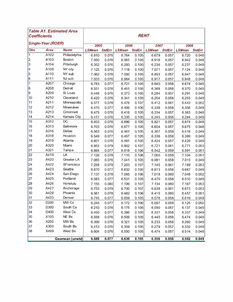
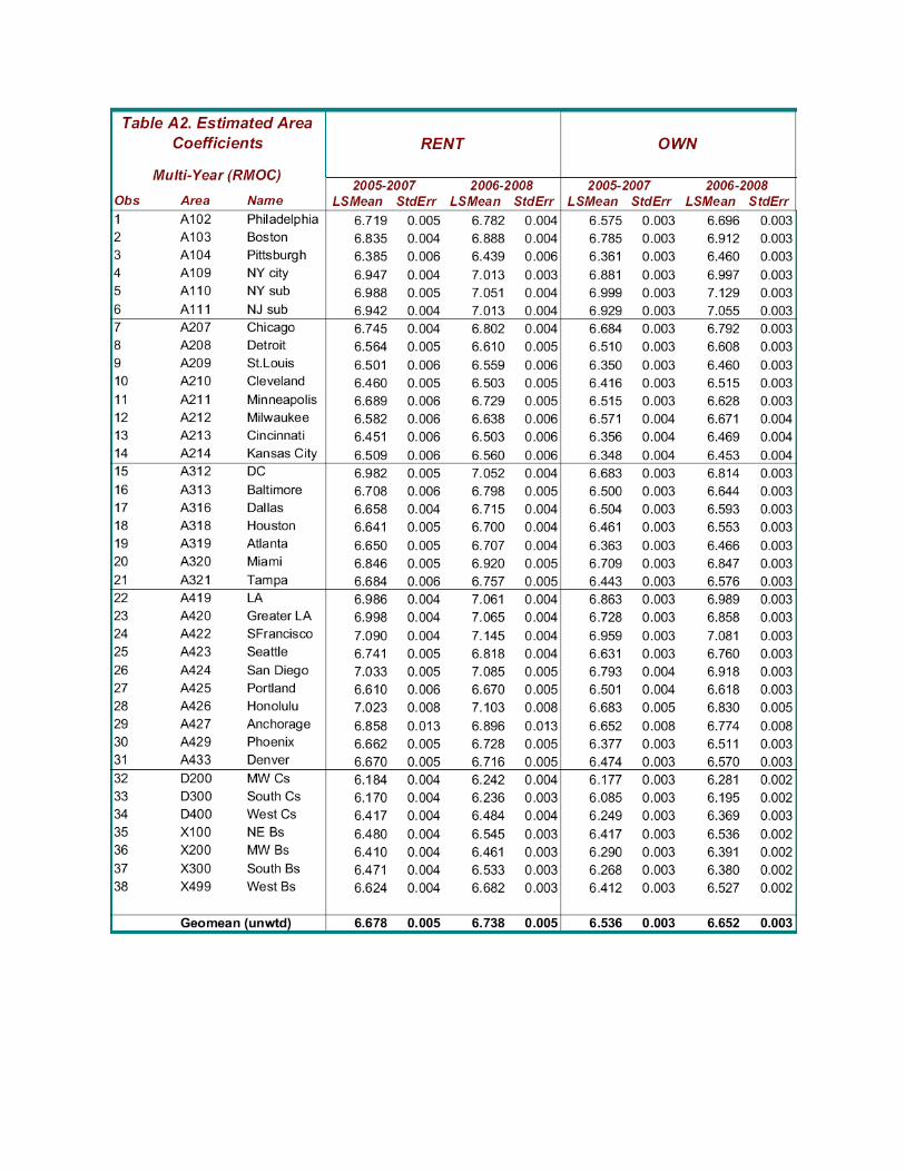
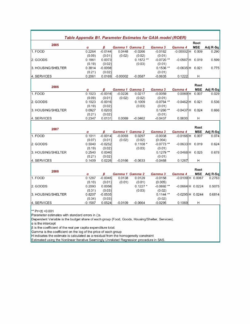
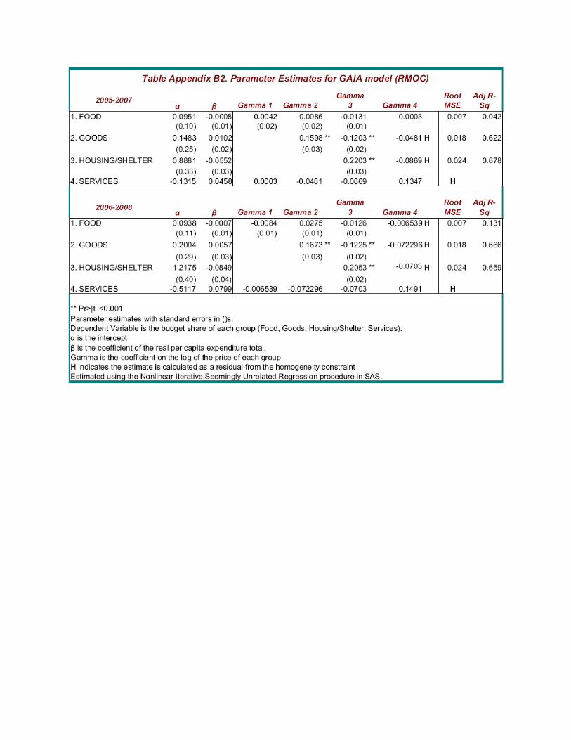
TECHNICAL APPENDIX

Algorithm for estimating GAIA World Prices

Let p denote an N×1 vector of logarithms of prices and let y0 denote the logarithm of nominal

total expenditures in period 0. Then the AIDS expenditure function evaluated at period 0 utility

u0 is:

ln e(p,u0) = αp + 0.5 p′γp + u0 exp(p′β)

If the observed prices of goods 1 to N in area i are pi0, the income that holds utility constant at ui0

when prices change to p is e(p,ui0), where ui0 = (yi0 – αpi0 + 0.5 pi0′γpi0) exp(–pi0′β). Therefore:

ln e(p,u0) = αp + 0.5 p′γp + (y0 – αp0 + 0.5 p0′γp0)exp(p – p0)′β

The theoretical restrictions of homogeneity of degree 1 in prices and symmetry of the Slutsky

matrix of own and cross price elasticities implies that the elements of α sum to 1, the matrix γ is

symmetric, with the elements of each row or of each column summing to 0, and the elements of

β sum to 0. Let γ1 denote the first row of the symmetric matrix γ, with α1 and β1 the first

elements of the vectors α and β. The predicted shares for goods 1 to N in area i at income

e(p,ui0) are:

wi1(p) = α1 + γ1p + β1(yi0 – αpi0 + 0.5 pi0′γpi0) exp[(p – pi0)′β]

wi2(p) = α2 + γ2p + β2(yi0 – αpi0 + 0.5 pi0′γpi0) exp[(p – pi0)′β]

…

wiN(p) = αΝ + γΝp + βΝ(yi0 – αpi0 + 0.5 pi0′γpi0) exp[(p – pi0)′β]

Let Ωi be the population of area i. Then the predicted total expenditures on good 1 in area i at

prices p are wi1(p)[e(p,ui0)Ni] and the predicted quantities in area i at prices p are:

Qi1(p) = wi1(p)[e(p,ui0) Ωi]/p1

…

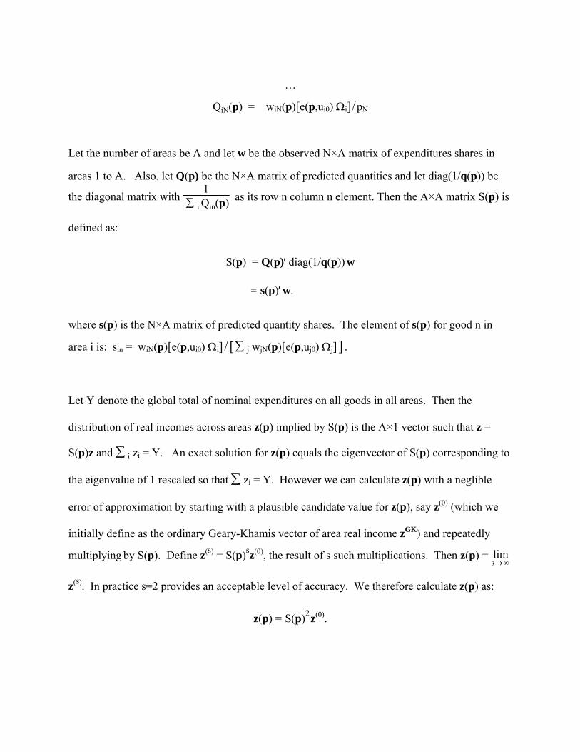
QiN(p) = wiN(p)[e(p,ui0) Ωi]/pN

Let the number of areas be A and let w be the observed N×A matrix of expenditures shares in

areas 1 to A. Also, let Q(p) be the N×A matrix of predicted quantities and let diag(1/q(p)) be

the diagonal matrix with 1

∑ i Qin(p) as its row n column n element. Then the A×A matrix S(p) is

defined as:

S(p) = Q(p)′ diag(1/q(p)) w

= s(p)′w.

where s(p) is the N×A matrix of predicted quantity shares. The element of s(p) for good n in

area i is: sin = wiN(p)[e(p,ui0) Ωi] / [∑ j wjN(p)[e(p,uj0) Ωj] ] .

Let Y denote the global total of nominal expenditures on all goods in all areas. Then the

distribution of real incomes across areas z(p) implied by S(p) is the A×1 vector such that z =

S(p)z and ∑ i zi = Y. An exact solution for z(p) equals the eigenvector of S(p) corresponding to

the eigenvalue of 1 rescaled so that ∑ zi = Y. However we can calculate z(p) with a neglible

error of approximation by starting with a plausible candidate value for z(p), say z(0) (which we

initially define as the ordinary Geary-Khamis vector of area real income zGK) and repeatedly

multiplying by S(p). Define z(s) = S(p)sz(0), the result of s such multiplications. Then z(p) = lims → ∞

z(s). In practice s=2 provides an acceptable level of accuracy. We therefore calculate z(p) as:

z(p) = S(p)2z(0).

Next define Π as the vector of ratios of “world” total expenditures on each good to “world” total

quantities consumed of each good:

Π(p) = diag(1/q(p)) w z(p)

= diag(1/q(p)) w S(p)2z(0).

If Πn is the nth element of Π(p) (the “world” price of good n), then Πn = [∑ i wni zi]/[∑ i Qni ].

The GAIA world price vector pGAIA is the p such that Π(p) = p. To solve for pGAIA, let D(p) be

the matrix of derivatives of Π(p) evaluated at p; element i,j of this matrix Dij = ∂Πi /∂pj. In

practice, we use numerical methods to estimate D(p).

Note that if Δp is the adjustment to our guess for p, then ΔΠ ≈ DΔp. As a result, if Π – p is the

error in our guess for pGAIA, the change in this error when we adjust our guess by Δp

approximately equals (D – I) Δp. If p(0) is our guess for pGAIA, we therefore choose Δp such that

–[Π(p(0)) – p(0)] = (D – I) Δp

or

Δp = –[D – I]−1 [Π(p(0)) – p(0)].

We begin with the ordinary Geary-Khamis prices pGK as the initial guess for pGAIA, and then

update this guess by:

p(1) = pGK – [D(pGK)– I]−1 [Π(pGK) – pGK]

p(2) = p(1) – [D(p(1))– I]−1 [Π(p(1)) – p(1)]

Iteration ceases when for every good n, Πn – pn < 10− 6 . In practice, this occurred after two

iterations.

Documents

Comparing the Consistency of Price Parities for Regions of ... · In our previous RPP estimates, we used the only the CPI data, that is, the Rents and Owners’ Equivalent Rent observations