Comparing Solution Methods for

Dynamic Equilibrium Economies∗

S. Boragan Aruoba

University of Pennsylvania

Jesús Fernández-Villaverde

University of Pennsylvania

Juan F. Rubio-Ramírez

Federal Reserve Bank of Atlanta

November 23, 2003

Abstract

This paper compares solution methods for dynamic equilibrium economies. Wecompute and simulate the stochastic neoclassical growth model with leisure choiceusing Undetermined Coefficients in levels and in logs, Finite Elements, ChebyshevPolynomials, Second and Fifth Order Perturbations and Value Function Iterationfor several calibrations. We document the performance of the methods in terms ofcomputing time, implementation complexity and accuracy and we present someconclusions about our preferred approaches based on the reported evidence.Key words: Dynamic Equilibrium Economies, Computational Methods, Linear

and Nonlinear Solution Methods.JEL classifications: C63, C68, E37.

∗Corresponding Author: Jesús Fernández-Villaverde, Department of Economics, 160 McNeil Building,3718 Locust Walk, University of Pennsylvania, Philadelphia, PA 19104. E-mail: jesusfv@econ.upenn.edu.We thank José Victor Ríos-Rull, Stephanie Schmitt-Grohé and participants at several seminars for usefulcomments, Kenneth Judd for encouragement to study perturbation methods further and Mark Fisher forcrucial help with Mathematica idiosyncrasies. Beyond the usual disclaimer, we must notice that any viewsexpressed herein are those of the authors and not necessarily those of the Federal Reserve Bank of Atlantaor of the Federal Reserve System.

1

1. Introduction

This paper addresses the following question: how different are the computational answers

provided by alternative solution methods for dynamic equilibrium economies?

Most dynamic equilibrium models do not have an analytic, closed-form solution and we

need to use numerical methods to approximate their behavior. There are a number of pro-

cedures to undertake this task (see Judd, 1998 or Marimón and Scott, 1999). However it

is difficult to assess a priori how the quantitative characteristics of the computed equilib-

rium paths change when we move from one solution approach to another. Also the relative

accuracies of the approximated equilibria are not well understood.

The properties of a solution method are not only of theoretical interest but crucial to

assess how reliable the answers provided by quantitative exercises are. For example if we

state, as in the classical measurement by Kydland and Prescott (1982), that the productivity

shocks account for seventy percent of the fluctuations of the U.S. economy, we want to know

that this number is not a by-product of numerical error. Similarly if we use the equilibrium

model for estimation purposes we need an approximation that does not introduce bias in the

estimates but yet is quick enough to make the exercise feasible.

Over 15 years ago a group of researchers compared solution methods for the stochastic

growth model without leisure choice (see Taylor and Uhlig, 1990 and the companion papers).

Since then, a number of nonlinear solution methods — several versions of projection (Judd,

1992 and McGrattan, 1999) and perturbation procedures (Judd and Guu, 1997) — have been

proposed as alternatives to more traditional (and relatively simpler) linear approaches and

to Value Function Iteration. However, little is known about the relative performance of the

new methods.1 This is unfortunate since these new methods, built on the long experience of

applied mathematics, promise superior performance. This paper tries to fill part of this gap

in the literature.

To do so, we use the canonical stochastic neoclassical growth model with leisure choice.

We understand that our findings are conditional on this concrete choice and that this paper

cannot substitute the close examination that each particular problem deserves. The hope is

1For the stochastic growth model we are only aware of the comparison between Chebyshev Polynomialsand different versions of the dynamic programming algorithm and policy iteration undertaken by Santos(1999) and Benítez-Silva et al. (2000). However those two paper (except one case in Santos, 1999) only dealwith the model with full depreciation and never with the other nonlinear methods. In a related contribution,Christiano and Fisher, 2000, study the performance of projection methods when dealing with models withoccasionally binding constraints.

2

that, at least partially, the experiences learned from this application could be useful for other

models. In that sense we follow from an old tradition in numerical analysis that emphasizes

the usefulness of comparing the performance of algorithms in well know test problems.

Why do we choose the stochastic neoclassical growth model as our test problem? First,

because this model is the workhorse of modern macroeconomics (see Cooley, 1995). Any

lesson learned in this context is bound to be useful in a large class of applications. Second,

because it is simple, a fact that allows us to solve it with a wide range of methods. For example

a model with binding constraints would rule out perturbation methods. Third, because we

know a lot about the theoretical properties of the model, results that are useful interpreting

our results. Finally because there exist a current project organized by Den Haan, Judd and

Julliard to compare different solution methods in heterogeneous agents economies. We see

our paper as a complement of this project for the more classical class of problems involving

a representative agent.

We solve and simulate the model using two linear approximations (based on the lineariza-

tion of the model equilibrium conditions around the deterministic steady state in levels and in

logs) and five nonlinear approximations (Finite Elements, Chebyshev Polynomials and three

Perturbation Methods, 2nd order in levels, 2nd order in logs and 5th order in levels). We

also solve the model using Value Function Iteration with a multigrid scheme. The results of

the Value Function Iteration method are a natural benchmark given our knowledge about

the convergence and stability properties of the procedure (see Santos and Vigo, 1998 and

references therein).

We report results for a benchmark calibration of the model and for alternative calibrations

that change the variance of the productivity shock and the risk aversion. In that way we study

the performance of the methods both for a nearly linear case (the benchmark calibration)

and highly nonlinear cases (high variance/high risk aversion). In our simulations we keep a

fixed set of stochastic shocks common for all methods. That allows us to observe the dynamic

responses of the economy to the same driving process and how computed paths and their

moments differ for each approximation. We also assess the accuracy of the solution methods

by reporting Euler Equation errors in the spirit of Judd (1992).

Five main results deserve to be highlighted. First, Perturbation Methods deliver an

interesting compromise between accuracy, speed and programming burden. For example,

we show how a 5th order perturbation has an advantage in terms of accuracy over all other

solution methods for the benchmark calibration. We quantitatively assess how much and how

3

quickly perturbations deteriorate when we move away from the steady state (remember that

perturbation is a local method). Also we illustrate how the simulations display a tendency to

explode and the reasons for such behavior.

Second, since higher order perturbations display a much superior performance over linear

methods for a trivial marginal cost, we see a compelling reason to move some computations

currently undertaken with linear methods to at least a 2nd order approximation.

Third, even if the performance of linear methods is disappointing along a number of

dimensions, linearization in levels is preferred to log-linearization for both the benchmark

calibration and the highly nonlinear cases. This results is new and contradicts a common

practice based on the fact that the exact solution to the model with log utility, inelastic labor

and full depreciation is log-linear.

Fourth, the Finite Elements method performs very well for all parametrizations. It is

extremely stable and accurate over the range of the state space even for high values of the

risk aversion and the variance of the shock. This property is crucial in estimation procedures

where the accuracy is required to obtain unbiased estimates (see Fernández-Villaverde and

Rubio-Ramírez, 2003a). However it suffers from being probably the most complicated method

to implement in practice (although not the most intensive in computing time).

Fifth, Chebyshev polynomials share all the good results of the Finite Elements Method and

are easier to implement. Since the neoclassical growth model has smooth policy functions,

it is not surprising that Chebyshev polynomials do well in this application. However in a

model where policy functions have kinks (e.g. due to the presence of binding constraints as in

Christiano and Fisher, 2000), Finite Elements is likely to outperform Chebyshev polynomials.

Therefore, although our results depend on the particular model we have used, they should

encourage a wider use of Perturbation Methods, to suggest the reliance on Finite Elements

for problems that demand high accuracy and stability and support the progressive phasing

out of pure linearizations.

The rest of the paper is organized as follows. Section 2 presents the canonical stochastic

neoclassical growth model. Section 3 describes the different solution methods used to ap-

proximate the policy functions of the model. Section 4 presents the benchmark calibration

and alternative robustness calibrations. Section 5 reports numerical results and section 6

concludes. A technical appendix provides further details about all the different methods.

4

2. The Stochastic Neoclassical Growth Model

As mentioned above we use the basic model in modern macroeconomics, the stochastic neo-

classical growth model with leisure as our test model for comparing solution methods.2

Since the model is well known we only go through the minimum exposition required to fix

notation. There is a representative agent in the economy, whose preferences over stochastic

sequences of consumption and leisure are representable by the utility function

U = E0

∞Xt=1

βt−1

³cθt (1− lt)1−θ

´1−τ1− τ

where β ∈ (0, 1) is the discount factor, τ is the elasticity of intertemporal substitution, θcontrols labor supply and E0 is the conditional expectation operator.

There is one good in the economy, produced according to the aggregate production func-

tion yt = eztkαt l1−αt where kt is the aggregate capital stock, lt is aggregate labor and zt is a

stochastic process representing random technological progress. The technology follows the

process zt = ρzt−1+²t with |ρ| < 1 and ²t ∼ N (0,σ2). Capital evolves according to the law ofmotion kt+1 = (1−δ)kt+ it and the economy must satisfy the resource constraint yt = ct+ it.

Since both welfare theorems hold in this economy, we can solve directly for the social

planner’s problem where we maximize the utility of the household subject to the production

function, the evolution of the stochastic process, the law of motion for capital, the resource

constraint and some initial conditions k0 and z0.

The solution to this problem is fully characterized by the equilibrium conditions:

³cθt (1− lt)1−θ

´1−τct

= βEt

³cθt+1 (1− lt+1)1−θ

´1−τct+1

¡1 + αezt+1kα−1t+1 l

1−αt+1 − δ

¢ (1)

(1− θ)

³cθt (1− lt)1−θ

´1−τ1− lt = θ

³cθt (1− lt)1−θ

´1−τct

(1− α) eztkαt l−αt (2)

2An alternative could have been the growth model with log utility function, no leisure choice and totaldepreciation, a case where a simple closed form solution exists (see Sargent, 1987). However since it is difficultto extrapolate the lessons from this particular example into statements for the more general case, we preferto pay the cost of not having an explicit analytic solution. In addition, Santos (2000) shows how changes inthe curvature of the utility function influence the size of the Euler equation errors.

5

ct + kt+1 = eztkαt l

1−αt + (1− δ) kt (3)

zt = ρzt−1 + εt (4)

and the boundary condition c(0, zt) = 0. The first equation is the standard Euler equation

that relates current and future marginal utilities from consumption, the second one is the

static first order condition between labor and consumption and the last two equations are

the resource constraint of the economy and the law of motion of technology.

Solving for the equilibrium of this economy amounts to finding three policy functions

for next period’s capital k (·, ·), labor l (·, ·) and consumption c (·, ·) that deliver the optimalchoice of the variables as functions of the two state variables, capital and the technology level.

All the computational methods used below except for the value function iteration exploit

directly the equilibrium conditions. This characteristic makes the extension of the methods

to non-pareto optimal economies — where we need to solve directly for the market allocation

— straightforward. As a consequence we can export at least part of the intuition from the

computational results in the paper to a large class of economies.

3. Solution Methods

The system of equations listed above does not have a known analytical solution and we need

to use a numerical method to solve it.

The most direct approach is to attack the social planner’s problem directly using Value

Function Iteration. This procedure is safe and reliable and has useful convergence theorems

(Santos and Vigo, 1998). However it is extremely slow (see Rust, 1996 and 1997 for acceler-

ating algorithms) and suffers from a strong curse of the dimensionality. Also it is difficult to

use in non-pareto optimal economies (see Kydland, 1989).

Because of these problems, the development of new solution methods for dynamic equi-

librium models has been an important area of research in the last decades. These solution

methods can be linear or nonlinear. The first ones exploit the fact that many dynamic

equilibrium economies display behavior that is close to a linear law of motion.

The second group of methods correct the approximation for higher order terms. Two

popular alternatives among these nonlinear approaches are perturbation (Judd and Guu, 1997

and Schmitt-Grohé and Uribe, 2002) and projection methods (Judd, 1992 and McGrattan,

1999). These approaches are attractive because they are much faster than Value Function

6

Iteration while sharing their convergence properties. This point is not only of theoretical

importance but of key practical relevance. For instance in estimation problems, since an

intermediate step in order to evaluate the likelihood function of the economy is to solve for

the policy functions, we want to use a fast solution method since we may need to perform

a huge number of these evaluations for different parameter values. Convergence properties

assure us that, up to some fixed accuracy level, we are indeed getting the correct equilibrium

path for economy.

In this paper we compare eight different methods. As our linear method, we use Un-

determined Coefficients to solve for the unknown coefficients of the policy functions using

linearized versions of the equilibrium equations of the model, both in levels and in logs.3

For the nonlinear methods we compute a Finite Elements method, a spectral procedure with

Chebyshev Polynomials, three Perturbation Approaches (a 2nd order expansion in levels, a

5th order expansion in levels and a 2nd order expansion in logs) and Value Function Iteration.4

We now briefly describe each of these methods. For a more detailed explanation we

refer the reader to Uhlig (1999) (Undetermined Coefficients in levels and logs), McGrattan

(1999) (Finite Elements), Judd (1992) (Chebyshev Polynomials) and Judd and Guu (1997)

and Schmitt-Grohé and Uribe (2002) (Perturbation). The technical appendix provides many

more details about the procedures and the computational parameters choices. A companion

web page at http://www.econ.upenn.edu/~jesusfv/companion.htm posts on line all the

codes required to reproduce the computations.

3.1. Undetermined Coefficients in Levels

The idea of this approximation is to substitute the system of equilibrium conditions with a

linearized version of it. Linear policy functions with undetermined coefficients are plugged

in the linear system and we solve for the unknown coefficients (see Uhlig, 1999 for details).

Beyond simplicity and speed, the procedure also allows us to derive some analytical results

3Note that, subject to applicability, all different linear methods described in the literature -LinearQuadratic approximation (Kydland and Prescott, 1982), the Eigenvalue Decomposition (Blanchard and Kahn,1980 and King, Plosser and Rebelo, 2002), Generalized Schur Decomposition (Klein, 2000 or the QZ decom-position (Sims, 2002) among many others, should deliver the same results. The linear approximation of adifferentiable function is unique and invariant to differentiable parameters transformations. Our particularchoice of linear method is then irrelevant.

4We do not try to cover every single known method but rather to be selective and choose those methodsthat we find more promising based either on experience or on intuition from numerical analysis. Below wediscuss how some apparently excluded methods are particular cases of some of our approaches.

7

about the model (see Campbell, 1994).

If we linearize the set of equilibrium conditions (1)-(4) around the steady state value xss

of the variables xt we get the linear system5:

θ (1− τ)− 1css

(ct − css)− (1− τ) (1− θ)

1− lss (lt − lss) =

Et

θ(1−τ)−1

css(ct+1 − css) +

³β α(1−α)

lss

ysskss− (1−τ)(1−θ)

1−lss

´(lt+1 − lss)

+αβ yssksszt+1 + β α(α−1)yss

k2ss(kt+1 − kss)

1

css(ct − css) + 1

(1− lss) (lt − lss) = zt +α

kss(kt − kss)− α

lss(lt − lss)

(ct − css) + (kt+1 − kss) = yssµzt +

α

kss(kt − kss) + 1− α

lss(lt − lss)

¶+ (1− δ) (kt − kss)

zt = ρzt−1 + εt

Simplification and some algebra delivers:

Abkt+1 +Bbkt + Cblt +Dzt = 0Et³Gbkt+1 +Hbkt + Jblt+1 +Kblt + Lzt+1 +Mzt´ = 0

Etzt+1 = Nzt

where the coefficients A,B,C, ..., N are functions of the model parameters and bxt = xt− xss.Now we guess policy functions of the form bkt+1 = Pbkt+Qzt and blt = Rbkt+Szt, plug them

in the linear system and solve the resulting quadratic problem for the unknown coefficients

P , Q, R and S that imply a stable solution. Note that the procedure delivers a linear law

of motion for the choice variables that displays certainty equivalence (i.e. it does not depend

on σ). This point will be important when we discuss our results. The other variables in the

model are solved for using the linearized system and the computed policy functions.

3.2. Undetermined Coefficients in Logs

Since the exact solution of the stochastic neoclassical growth model in the case of log utility,

total depreciation and no leisure choice is loglinear, a large share of practitioners have fa-

vored the loglinearization of the equilibrium conditions of the model over linearization. Some

5See the technical appendix for a discussion of alternatives points for the linearization.

8

evidence in Christiano (1990) and Den Haan and Marcet (1994) suggest that this is the right

practice but the question is not completely settled. To cast light on this question and perform

a systematic comparison of both alternatives below, we repeat our undetermined coefficient

procedure in logs: we loglinearize the equilibrium conditions instead of linearizing them but

proceed otherwise as before.

In particular we take the equilibrium conditions of the model and we substitute each

variable xt by xssebxt and bxt = log xtxss. Then we linearize with respect to bxt around bxt = 0

(i.e. the steady state). After some algebra we get:

Abkt+1 +Bbkt + Cblt +Dzt = 0Et³Gbkt+1 +H bkt + Jblt+1 +Kblt + Lzt+1 +Mzt´ = 0

Etzt+1 = Nzt

where the coefficients A,B,C, ..., N are functions of the parameters of the model.

We guess policy functions of the form bkt+1 = Pbkt +Qzt and blt = Rbkt + Szt, plug them inthe linear system and solve for the unknown coefficients.6

3.3. Finite Elements Method

The Finite Elements Method (Hughes, 2000 and McGrattan, 1999) is the most widely used

general-purpose technique for numerical analysis in engineering and applied mathematics.

Beyond being conceptually simple and intuitive, the Finite Elements Method features several

interesting properties. First, it provides us a lot of flexibility in the grid generation: we

can create very small elements (and consequently very accurate approximations of the policy

function) in the neighborhood of the mean of the stationary distribution of capital and larger

ones in the areas of the state space less travelled. Second, large numbers of elements can

be handled to thanks to the sparsity of the problem. Third, the Finite Elements method

is well suited for implementation in parallel machines with the consequent scalability of the

problem.

The Finite Elements Method searches for a policy function for labor supply of the form

lfe¡k, z; θ

¢=P

i,j θijΨij (k, z) where Ψij (k, z) is a set of basis functions and θ is a vector of

6Alternatively we could have taken the coefficients from the linearization in levels and transform themusing a nonlinear change of variables and the Chain Rule. The results would be the same as the ones in thepaper. See Judd (2003) and Fernández-Villaverde and Rubio-Ramírez (2003b).

9

parameters to be determined. Note that given lfe¡k, z; θ

¢, the static first order condition and

the resource constraint imply two policy function c(k, z; lfe¡k, z; θ

¢) and k0

¡k, z; lfe

¡k, z; θ

¢¢for consumption and next period capital. The essence of the Finite Elements method is to

chose basis functions that are zero for most of the state space except a small part of it, an

interval in which they take a very simple form, typically linear.7

First we partition the state space Ω in a number of nonintersecting rectangles [ki, ki+1]×[zj, zj+1] where ki is the ith grid point for capital and zj is jth grid point for the technology

shock. As basis functions we set Ψij (k, z) = bΨi (k) eΨj (z) where

bΨi (k) =

k−ki

ki+1−ki if k ∈ [ki−1, ki]ki+1−kki+1−ki if k ∈ [ki, ki+1]

0 elsewhere

eΨj (z) =

z−zj

zj+1−zj if z ∈ [zj−1, zj]zj+1−zzj+1−zj if z ∈ [zj, zj+1]

0 elsewhere

Then we plug lfe¡k, z; θ

¢and c(k, z; lfe

¡k, z; θ

¢) and k0

¡k, z; lfe

¡k, z; θ

¢¢in the Euler

Equation to get a residual function R(kt, zt; θ).

A natural criterion for finding the θ unknowns is to minimize this residual function over

the state space given some weight function. To do sowe employ a Galerkin scheme where the

basis functions double as weights to get the nonlinear system of θ equationsZΩ

Ψi,j (k, z)R(k, z; θ)dzdk = 0 ∀i, j (5)

on our θ unknowns. Solving this system delivers our desired policy function lfe¡k, z; θ

¢from

which we can find all the other variables in the economy.8

7We can have more elaborated basis functions as Chebyshev polynomials and solve the resulting Spectral-Finite Elements problem. These type of schemes, known as the p-method are much less used than the so-calledh-method whereby the approximation error is reduced through successive mesh refinement.

8Note that policy function iteration (see for example Coleman, 1990) is just a particular case of the FiniteElements when we pick a collocation scheme in the points of an exogenously given grid, linear basis functionsand an iterative scheme to solve for the unknown coefficients. Experience from numerical analysis suggeststhat nonlinear solvers (as the simple Newton scheme that we used for our unknown coefficients) or multigridschemes outperform pure iterative algorithms (see Briggs, Henson, and McCormick, 2000). Also Galerkinweigthings are superior to collocation for Finite Elements (Boyd, 2001).

10

3.4. Spectral Method (Chebyshev Polynomials)

Like Finite Elements, spectral methods (Judd, 1992) search for a policy function of the form

lsm¡k, z; θ

¢=P

i,j θijΨij (k, z) where Ψij (k, z) is a set of basis functions and θ is a vector of

parameters to be determined. The difference with respect to the previous approach is that

the basis functions are (almost surely) nonzero, i.e. we search for a global solution instead of

pasting together local solutions as we did before.

Spectral methods have two main advantages over the Finite Elements method. First,

they are generally much easier to implement. Second, since we can easily handle a large

number of basis functions the accuracy of the procedure is potentially very high. The main

drawback of the procedure is that it approximates the true policy function globally. If the

policy function displays a rapidly changing local behavior, or kinks, the scheme may deliver

a poor approximation.

A common choice for the basis functions is to set the tensor Ψij (k, z) = bΨi (k) eΨj (z)

where bΨi (·) and eΨj (·) are Chebyshev polynomials (see Boyd, 2001 and Fornberg, 1998 forjustifications of this choice of basis functions). These polynomials can be recursively defined

by T0 (x) = 1, T1 (x) = 1 and for general n, Tn+1 (x) = 2Tn (x)− Tn−1 (x).9As in the previous case we use the two Euler Equations with the budget constraint substi-

tuted in to get a residual function R(kt, zt; θ). Instead of a Galerkin weighting, computational

experience (Fornberg, 1998) suggests that, for spectral methods, a collocation (also known as

pseudospectral) criterion delivers the best trade-off between accuracy and ability to handle

large number of basis functions. Collocation uses as weights the n × m dirac functions δj

with unit mass in n×m points (n from the roots of the last polynomial used in the capital

dimension and m from the points in Tauchen’s, 1986 approximation to the stochastic process

for technology). This scheme results in the nonlinear system of n×m equations

R(kij, zij; θ) = 0 for ∀ n×m collocation points (6)

in n×m unknowns. This system is easier to solve than (5) since we will have in general less

basis functions and we avoid the integral induced by the Galerkin weigthing.10

9The domain of the Chebyshev polynomials is [−1, 1]. Since our state space is different in general we usea linear mapping from [a, b] into [−1, 1].10Parametrized expectations (see Marcet and Lorenzoni, 1999 for a description) is a spectral method that

uses monomials (or exponents of) in the current states of the economy and montecarlo integration. Sincemonomials are highly collinear and determinist integration schemes are preferred for low dimensional problems

11

3.5. Perturbation

Perturbation methods (Judd and Guu, 1997 and Schmitt-Grohé and Uribe, 2002) build a

Taylor series expansion of the policy functions of the economy around some point of the state

space and a perturbation parameter set at zero. In our case we use the steady state value

of capital and productivity and the standard deviation of the innovation to the productivity

level σ.11

With these choices the policy functions take the form

cp(k, z,σ) =Xi,j,m

acijm (k − kss)i (z − zss)j σm

lp(k, z,σ) =Xi,j,m

alijm (k − kss)i (z − zss)j σm

k0p(k, z,σ) =Xi,j,m

akijm (k − kss)i (z − zss)j σm

where acijm =∂i+j+mc(k,z,σ)∂ki∂zj∂σm

¯kss,zss,0

, alijm =∂i+j+ml(k,z,σ)∂ki∂zj∂σm

¯kss,zss,0

and akijm =∂i+j+mk0(k,z,σ)

∂ki∂zj∂σm

¯kss,zss,0

are equal to the derivative of the policy functions evaluated at the steady state value of the

state variables and σ = 0.

The perturbation scheme works as follows. We take the model equilibrium conditions

(1)-(4) and substitute the unknown policy functions c(k, z,σ), l(k, z,σ) and k0(k, z,σ) in.

Then we take successive derivatives with respect to the k, z and σ. Since the equilibrium

conditions are equal to zero for any value of k, z and σ, a system created by their derivatives

of any order will also be equal to zero. Evaluating the derivatives at the steady state value

of the state variables and σ = 0 delivers a system of equations on the unknown coefficients

acijm, alijm and a

kijm.

The solution of these systems is simplified because of the recursive structure of the prob-

lem. The constant terms ac000, al000 and a

k000 are equal to the deterministic steady state for

consumption, labor and capital. Substituting these terms in the system of first derivatives

of the equilibrium conditions generates a quadratic matrix-equation on the first order terms

of the policy function (by nth order terms of the policy function we mean aqijm such that

over montecarlo approaches (Geweke, 1996), we stick with Chebyshev polynomials as our favorite spectralapproximation. See Christiano and Fisher (2000) for a thorough explanation.11The choice of perturbation parameter is model-dependent. Either the standard deviation (for discrete

time models) or the variance (for continuous time models) are good candidates for stochastic equilibriumeconomies.

12

i + j + m = n for q = c, l, k). Out of the two solutions we pick the one that gives us the

stable path of the model

The next step is to plug in the system created by the second order expansion of the

equilibrium conditions the known coefficients from the previous two steps. This step generates

a linear system in the 2nd order terms of the policy function that is trivial to solve.

Iterating in the procedure (taking a one higher order derivative, substituting previously

found coefficients and solving for the new unknown coefficients), we would see that all the

higher than 2nd order coefficients are just the solution to linear systems. The intuition of why

only the system of first derivatives is quadratic is as follows: the stochastic neoclassical growth

model has two saddle paths, once we have picked the right path with the stable solution in

the first order approximation, all the other terms are just refinements of this path.

The burden of the method is taking all the required derivatives, since the systems of

equations are always linear. Paper and pencil become virtually infeasible after the second

derivatives. Gaspar and Judd (1997) show that higher order numerical derivatives accumulate

enough errors to prevent their use. An alternative is to work symbolic manipulation software

as Mathematica.12 However that means that we lose the speed of low level languages as C++

or Fortran 95. In the absence of publicly available libraries for analytic derivation in this

languages, the required use of less powerful software limits the applicability of perturbation.

Perturbations only deliver an asymptotically correct expression around the deterministic

steady state for the policy function but given the positive experience of asymptotic approx-

imations in other fields of applied mathematics, there is the potential for good nonlocal

behavior (see Bender and Orszag, 1999).

When implementing the approximation we face two choices. First we need to decide

the order of the perturbation. We choose 2nd and 5th order perturbations. Second order

approximations have received attention because of the easiness of their computation (see

Schmitt-Grohé and Uribe, 2002 and Sims, 2000) and we find of interest to assess how much

gain is obtained by this simple correction of the linear policy functions. Then we pick a high

order approximation. After the fifth order the coefficients are nearly equal to the machine

zero (in a 32-bits architecture of the standards PCs) and further terms do not add much to the

behavior of the approximation. The second choice is whether to undertake our perturbation

12For second order perturbations we can also use the Matlab based programs by Schmitt-Grohé and Uribe(2002) and Sims (2000). For higher order perturbations we need Mathematica because the symbolic toolboxof Matlab cannot handle more than the second derivatives of abstract functions.

13

in levels and logs. We performed both cases but because of space considerations we only

present results in levels except for the 2nd order approximation for the high variance/high

risk aversion case where we report results both in levels and in logs. The omitted results were

nearly indistinguishable from perturbations in levels since the additional quadratic term in

both expansions corrected for the differences in the linear term between levels and logs.

3.6. Value Function Iteration

Finally we solve the model using value function iteration. Since the dynamic algorithm is

well known we only present a sparse discussion.

We generate a grid for capital and we discretize the productivity level using the method

proposed by Tauchen (1986). We use a multigrid scheme where the last step has a uniform

one million points grid, with 25000 points for capital and 40 for the productivity level. Then

for each point in the grid we iteratively compute the Bellman operator:

TV (k, z) = maxc>0,0<l<1,k0>0

³cθ (1− l)1−θ

´1−τ1− τ

+ βEV (k0, z0|z) (7)

c+ k0 = exp (z) kαl1−α + (1− δ) k (8)

z0 = ρz + ε (9)

We explore different interpolation schemes (linear, quadratic and Schumaker, 1993) for

values of the function outside the grid until convergence and report the ones with better

performance.

4. Calibration: Benchmarks Case and Robustness

To make our comparison results as useful as possible we pick a benchmark calibration and

we explore how those results change as we move to different “unrealistic” calibrations.

We select the benchmark calibration values for the stochastic neoclassical growth model as

follows. The discount factor β = 0.9896matches an annual interest rate of 4% (see McGrattan

and Prescott, 2000 for a justification of this number based on their measure of the return on

capital and on the risk-free rate of inflation-protected U.S. Treasury bonds). The risk aversion

τ = 2 is a common choice in the literature. θ = 0.357 matches the microeconomic evidence

of labor supply to 31% of available time in the deterministic steady state. We set α = 0.4 to

14

match labor share of national income (after the adjustments to National Income and Product

Accounts suggested by Cooley and Prescott, 1995). The depreciation rate δ = 0.0196 fixes

the investment/output ratio and ρ = 0.95 and σ = 0.007 match the stochastic properties of

the Solow residual of the U.S. economy. The chosen values are summarized in table 4.1.

Table 4.1: Calibrated Parameters

Parameter β τ θ α δ ρ σ

Value 0.9896 2.0 0.357 0.4 0.0196 0.95 0.007

To check robustness, we repeat our analysis for five other calibrations. As explained in

the introduction this analysis allows us to study the relative performance of the methods

both for a nearly linear case (the benchmark calibration) and for highly nonlinear cases (high

variance/high risk aversion). We increase the risk aversion to 10 and 50 and the standard

deviation of the productivity shock to 0.035. Although below we concentrate on the results

for the benchmark and the extreme case, the intermediate cases are important to check that

our comparison across calibrations does not hide non-monotonicities. Table 4.2. summarizes

our different cases.

Table 4.2: Sensitivity Analysis

case σ = 0.007 σ = 0.035

τ = 2 Benchmark Intermediate Case 3

τ = 10 Intermediate Case 1 Intermediate Case 4

τ = 50 Intermediate Case 2 Extreme

Also we briefly discuss some results for the deterministic case σ = 0 since they well help

us understand some characteristics of the proposed methods.

5. Numerical Results

In this section we report results from our different methods and calibrations. We concentrate

on the benchmark and extreme calibrations, reporting the intermediate cases when they

clarify the argument.13 First we present and discuss the computed policy functions. Second

we show some simulations. Third we perform the χ2 accuracy test proposed by Den Haan

and Marcet (1990), we report the Euler Equation Errors as in Judd (1992) and Judd and

Guu (1997) and a weighting of the Euler Equation error using the simulated distributions.

Finally we discuss some details about implementation and computing time.

13All additional results are available upon request.

15

5.1. Policy Functions

One of the first outputs of the computation is the policy functions. We plot the decision

rules for labor supply when z = 0 over a capital interval centered around the deterministic

steady state level of capital for the benchmark calibration in Figure 5.1.1 and for investment

in Figure 5.1.2.14 Since many of the nonlinear methods provide indistinguishable answers we

only observe four colors in both figures. Labor supply is very similar in all methods, especially

in the neighborhood of 23.14, the deterministic steady state level of capital. Only far away

from that neighborhood we appreciate any relevant difference.15 A similar description applies

to the policy rule for investment except for the loglinear approximation where the rule is

pushed away from the other ones for low and high capital. The difference is big enough that

even the monotonicity of the policy function is lost. In this behavior rests already a hint of

the problems with loglinearization that we will discuss below.

Dramatic differences appear as we begin to increase risk aversion and the variance of the

shock. The biggest discrepancy is for the extreme calibration. The policy functions for this

case are presented in Figures 5.1.3 and 5.1.4. In these figures we change the interval reported

because, due to the risk aversion/high variance of the calibration, the equilibrium paths will

fluctuate around much higher levels of capital (between 30 and 45) when the solution method

accounts for that high variance (i.e. all except linearizations).

We highlight several results. First, the linear and loglinear policy functions deviate from

all the other ones: they imply much less labor (around 10%) and investment (up to 30%)

than the group of nonlinear methods. This difference in level is due to the lack of correction

for increased variance of the technology shock by these two approximations since they are

certainty-equivalent. This shows how linearization and certainty equivalence produce biased

results. Second just correcting for quadratic terms in the 2nd order perturbation allows to

get the right level of the policy functions. This is another key point in our argument in favor

of phasing out linearizations and substitute them by at least 2nd order perturbations. Third,

the policy function for labor and investment approximated by the 5th order perturbation

changes from concavity into convexity for values of capital bigger than 45. (contrary to the

theoretical results) This change of slope will cause problems below in our simulations.16

14Similar figures could be plotted for other values of z. We omit them because of space considerations.15We must be cautious mapping differences in choices into differences in utility (see Santos, 2000). The

Euler Error function below provides a better view of the welfare consequences of different approximations.16One last result is that the policy functions have a positive slope. This is because households are so

risk-adverse that they want to work hard when capital is high to accumulate even more capital and insure

16

5.2. Simulations

Practitioners often rely in statistics from simulated paths of the economy. We computed 1000

simulations of 500 observations each for all different methods. To make comparisons mean-

ingful we keep the productivity shock constant across methods for each particular simulation.

We plot in Figures 5.2.1-5.2.4 the histograms for output, capital, labor and consumption

for the different methods for the benchmark calibration (where we have dropped the first

100 observations of each simulation as a burn-in period). As we could have suspected after

looking at the policy functions, the histograms suggest that the different methods deliver

basically the same behavior for the economy. That impression is reinforced by Figures 5.2.5

and 5.2.6 where we plot the paths of output and capital for one randomly chosen simulation.

All paths are roughly equal. This similarity of the simulation paths causes that the business

cycle statistics for the model under different solution methods (not reported here but available

upon request) to be nearly identical.

We repeat the same exercise for the extreme calibration in Figures 5.2.7-10. We see three

groups: first the two linear methods, second the perturbations and finally the three global

methods (value function, Finite Elements and Chebyshev). The last two groups have the

histograms shifted to the right: much more capital is accumulated and more labor supplied by

all the methods that allow for corrections by variance. For example the empirical distributions

of nonlinear methods accumulate a large percentage of their mass between 40 and 50 while

the linear methods rarely visit that region. Even different non-linear methods provide quite

a diverse description of the behavior of economy. In particular the three global methods are

in a group among themselves (nearly on top of each other) separated from perturbations that

lack enough variance. Figures 5.2.11 and 5.2.12 plot a simulation of the economy randomly

chosen where the differences in output and capital are easy to visualize.

Higher risk aversion/high variance also have an impact for business cycle statistics. For

example investment is three times more volatile in the linear simulation than with Finite

Elements despite the filtering of the data.

The simulations show an important drawback of using perturbations to characterize equi-

librium economies. For example in 39 simulations out of the 1000 (not shown on the his-

tograms) 5th order perturbation generated a capital that exploded. The reason for that

abnormal behavior is the change in the slope of the policy functions reported above. When

against future bad shocks. Numerically we found that the change in slope occurs for τ around 40.

17

the economy begins to travel that part of the policy functions the simulation falls in an un-

stable path and the results need to be disregarded. This instability property is an important

problem of perturbations that may limit its use.17

5.3. A χ2 Accuracy Test

From our previous discussion it is clear that the consequences for simulated equilibrium paths

of using different methods are important. A crucial step in our comparison is then the analysis

of accuracy of the computed approximations to figure it out which one we should prefer.

We begin that investigation implementing the χ2−test proposed by Den Haan and Marcet(1990). The authors noted that if the equilibrium of the economy is characterized by a system

of equations f (yt) = Et (φ (yt+1, yt+2, ..)) where the vector yt contains all the n variables that

describe the economy at time t, f : <n → <m and φ : <n × <∞ → <m are known functionsand Et (·) represent the conditional expectation operator, then

Et (ut+1 ⊗ h (xt)) = 0 (10)

for any vector xt measurable with respect to t with ut+1 = φ (yt+1, yt+2, ..) − f (yt) andh : <k → <q being an arbitrary function.Given one of our simulated series of length T from the method i in previous section,

yitTt=1, we can find©uit+1, x

it

ªTt=1

and compute the sample analog of (10):

BiT =1

T

TXt=1

uit+1 ⊗ h¡xit¢

(11)

Clearly (11) would converge to zero as T increases almost surely if the solution method

were exact. However, given the fact that we only have numerical methods to solve the

problem, this may not be the case in general. However the statistic T (BiT )0(AiT )

−1BiT where

AiT is a consistent estimate of the matrixP∞

t=−∞Et£(ut+1 ⊗ h (xt)) (ut+1 ⊗ h (xt))0

¤given

solution method i, converges in distribution to a χ2 with qm degrees of freedom under the

null that (10) holds. Values of the test above the critical value can be interpreted as evidence

against the accuracy of the solution.

17We also had problems in the high risk aversion/high variance with 1 simulation in the 2nd order pertur-bations, 1 simulation in the log 2nd order perturbations and 65 simulation in the linearization in levels (thoselast ones because capital goes below zero). In the benchmark calibration we did not have any problems.

18

Since any solution method is an approximation, as T grows we will eventually always

reject the null. To control for this problem, we can repeat the test for many simulations and

report the percentage of statistics in the upper and lower critical 5% of the distribution. If

the solution provides a good approximation, both percentages should be close to 5%.

We report results for the benchmark calibration in Table 5.3.1 and plot the Empirical CDF

in Figure 5.3.1.18 All the methods perform similarly and reasonably close to the nominal

coverages,with a small bias towards the right of the distribution. Also, and contrary to

some previous findings for simpler models (as reported by Den Haan and Marcet, 1994 and

Christiano, 1990) it is not clear that we should prefer loglinearization to linearization.

Table 5.3.1: χ2 Accuracy Test, τ = 2/σ = 0.007

Less than 5% More than 95%

Linear 3.10 5.40

Log-Linear 3.90 6.40

Finite Elements 3.00 5.30

Chebyshev 3.00 5.40

Perturbation 2 3.00 5.30

Perturbation 5 3.00 5.40

Value Function 2.80 5.70

We present the results for the extreme case in table 5.3.2 and Figure 5.3.2.19 Now the

performance of the linear methods deteriorates enormously, with quite unacceptable coverages

(although again linearization in levels is no worse than loglinearization). On the other hand

nonlinear methods deliver quite a good performance, with very reasonable coverages on the

upper tail (except 2nd order perturbations). The lower tail behavior is poor for all methods.

18We use a constant, kt, kt−1, kt−2 and zt as our instruments, 3 lags and a Newey-West Estimator of thematrix of variances-covariances (Newey and West, 1987).19The problematic simulations as described above are not included in these computations.

19

Table 5.3.2: χ2 Accuracy Test, τ = 50/σ = 0.035

Less than 5% More than 95%

Linear 0.43 23.42

Log-Linear 0.40 28.10

Finite Elements 1.10 5.70

Chebyshev 1.00 5.20

Perturbation 2 0.90 12.71

Perturbation 2-Log 0.80 22.22

Perturbation 5 1.56 4.79

Value Function 0.80 4.50

5.4. Non Local Accuracy test

The previous test is a simple procedure to evaluate the accuracy of the solution procedure.

That approach may suffer, however, from three problems. First, since all methods are just

approximations the test will display poor power. Second orthogonal residuals can be compat-

ible with large deviations from the optimal policy. Third, by its design the model will spend

most of the time in those regions where the density of the stationary distribution is higher.

Often it is important to assess the accuracy of a model far away from the steady state as in

estimation procedures where we want to explore the global shape of the likelihood function.

Judd (1992) proposes to determine the quality of the solution method defining normalized

Euler Equation Errors. First note that in our model the intertemporal condition

u0c (c (kt , zt) , l (kt , zt)) = βEt u0c (c (k (kt , zt) , zt+1) , l (k (kt , zt) , zt+1))R (kt , zt , zt+1)(12)

where R (kt , zt, zt+1) =¡1 + αezt+1k (kt , zt)

α−1 l (k (kt , zt) , zt+1)1−α − δ

¢is the gross return

rate of capital, should hold exactly for given kt and zt.

Since the solution methods used are only approximations, (12) will not hold exactly when

evaluated using the computed decision rules. Instead, for solution method i with associated

policy rules ci (· , ·) , li (· , ·) and ki (· , ·) and the implied gross return of capital Ri (kt , zt, zt+1),we can define the Euler Equation error function EEi (· , ·) as:

EEi (kt , zt) ≡ 1−

ÃβEtu0c(ci(ki(kt ,zt) ,zt+1),li(ki(kt ,zt) ,zt+1))Ri(kt ,zt,zt+1)

θ(1−li(ki(kt ,zt) ,zt+1))(1−θ)(1−τ)

! 1θ(1−τ)−1

ci (kt , zt)(13)

20

This function determines the (unit free) error in the Euler Equation as a fraction of the

consumption given the current states kt and zt and solution method i. Judd and Guu (1997)

interpret this error as the relative optimization error incurred by the use of the approximated

policy rule. For instance if EEi (kt , zt) = 0.01, then the agent is making a $1.00 mistake for

each $100 spent. In comparison, EEi (kt , zt) = 1e−8 implies that the agent is making a 1

cent mistake for each million of dollars spent.

The Euler Equation error is also important because we know that under certain conditions,

the approximation error of the policy function is of the same order of magnitude as the size

of the Euler equation error and correspondingly the change in welfare is of the square order

of the Euler equation error (Santos, 2000).

Figures 5.4.1-5.4.10 present the Euler Equation Errors for our benchmark calibration.

Figure 5.4.1 shows the results for the linear approximation to the equilibrium conditions

for capital between 70% and 130% of the deterministic steady state level (23.14) and for a

range of technology shocks from -0.065 to 0.065 (with zero being the level of technology in the

deterministic case).20 We plot the absolute errors in base 10 logarithms to ease interpretation.

A value of -3 means $1 mistake for each $1000, a value of -4 a $1 mistake for each $10000 and

so on. As intuition would suggest the error is much lower around the central regions, closer

to the point around which we make our linear expansion. The quality of the approximation

deteriorates as we move away from the central regions and quickly reaches -3. Figure 5.4.2

follows the same convention and plots the errors of the loglinear approximation. We can

see a pattern with two narrow valleys of high accuracy surrendered by regions with worse

errors. The origin of these valleys will be explained below. As in the case of the χ2-test, from

the comparison of figures 5.4.1 and 5.4.2 it is not obvious that we should prefer loglinear

approximations to straight linearizations.

The next two figures display the results for Finite Elements (figure 5.4.3) and Chebyshev

polynomials (figure 5.4.4). Finite Elements delivers a very robust performance along the state

space, specially for technology shocks between -0.02 and 0.02 (our mesh is finer in this region)

where the errors fluctuate around -7 (with some much better points around the nodes of the

elements). Only for large shocks (where our mesh is coarser) the performance of finite elements

deteriorates. Chebyshev polynomials emerge from figure 5.4.4 as a very competitive solution

method: the error is consistently below -8. Given the much lower computational burden of

Chebyshev polynomials versus Finite Elements, the result is encouraging for spectral methods.

200.065 corresponds to roughly 99.5th percentile of the normal distribution given our parameterization.

21

Figures 5.4.5 and 5.4.6 present the Euler Equation Errors for the 2nd and 5th order per-

turbations. Figure 5.4.5 proves how we can strongly improve the accuracy of the solution

over a linear approximation paying only a trivial additional cost that delivers a result nearly

as good as Finite Elements. Correcting for variance and quadratic terms reduces Euler errors

by an order of magnitude over the results from linear methods. The 5th order approximation

performance is superb. Over the whole range, its error is less than -7 and in the central

regions up to —8.

Finally Figure 5.4.7 graphs the Euler Equation Errors for the Value Function iteration

that fluctuate around -5 with the ups and downs induced by the grid and the expected uniform

performance over the state space. It is surprising that even for a very fine grid (one million

points over a relatively small part of the state space) the Value Function approximation is not

overwhelmingly accurate. This result illustrates a potential shortcoming of those exercises

that compare the performance of a solution algorithm with the results of Value Function

iteration as the “true” solution.

To get a better view of the relative performance of each approximation and since plotting

all the error functions in a same plot is cumbersome, Figure 5.4.8 displays a transversal cut of

the errors when the technology is equal to zero. Here we can see many of the same results we

just discussed. The loglinear approximation is worse than the linearization except at the two

valleys. Finite Elements and Chebyshev polynomials perform much better than the linear

methods (three orders of magnitude even at the steady state) and perturbations’ accuracy is

impressive. Other transversal cuts at different technology levels reveal similar patterns.

To explore further the origin of the errors we plot in figure 5.4.9 the level of the Euler

Equation errors at z = 0. With this graph we can explain the two valleys of the loglineariza-

tion: at the deterministic steady state level of capital loglinearization induces a negative bias

in the Euler Equation while the errors tend to grow quickly away from it. The two valleys

are just the two neighborhoods where the parabola crosses the zero. The parabola of the

linearization is always positive (something by itself neutral) but much flatter. Our reading of

these shapes is that linearization may be better than loglinearization after all. Figure 5.4.10

plots the same figure eliminating the two linear approximations to zoom the behavior of the

error of all the other methods, that are of a much smaller magnitude.

We can combine the information from the simulations and from the Euler Equation Errors

integrating the (absolute) Euler Equation errors using the computed distribution. This exer-

cise is a generalization of the Den Haan-Marcet test where instead of using the conditional

22

expectation operator we estimate an unconditional expectation using the population distrib-

ution. This integral is a welfare measure of the loss induced by the use of the approximating

method over the exact solution.

Table 5.4.1: Integral of the Euler Errors (x10−4)

Linear 0.2291

Log-Linear 0.6306

Finite Elements 0.0537

Chebyshev 0.0369

Perturbation 2 0.0481

Perturbation 5 0.0369

Value Function 0.0224

Results are presented in Table 5.4.1.21 Our interpretation of the numbers show that lin-

earization in levels must be preferred over loglinearization for the benchmark calibration of the

stochastic neoclassical growth model with leisure and that the performance of perturbation

methods is excellent.

Another view of the same information is provided by Figure 5.4.11 where we plot a

nonparametric estimate of the marginal distribution of capital around z = 0 and the Euler

Equation Errors around z = 0. This figure allow us to get a feeling of where the stationary

distribution is spending time and how big are the Euler Equation errors there.

The problems of linearization are not as much due to the presence of uncertainty but to

the curvature of the exact policy functions and second that the loglinear approximation is

clearly inferior to a linearization in levels. Even with no uncertainty the Euler Equation Errors

of the linear methods (not reported here) are very poor in comparison with the nonlinear

procedures.

Figures 5.4.12-5.4.20 display results for the extreme calibration τ = 50 and σ = 0.035

(again we have changed the capital interval to make it representative). Figure 5.4.12 shows

the huge errors of the linear approximation, of order -3 in the relevant parts of the state space.

Figure 5.4.13 plots even worse error for the log-linear approximation, of around -2. Figure

5.4.14 shows how Finite Elements still displays a robust and stable behavior over the state

space. This result is not a big surprise since the global character of the method allows it to

21We use the distribution from Value Function Iteration. Since the distributions are nearly identical for allmethods, the table is also nearly the same if we use any other distributions. The only caveat is that usingthat distribution slightly favors the integral from Value Function Iterations.

23

pick the strong nonlinearities induced by high risk aversion and high variance. Chebyshev’s

performance is also very good and delivers similar accuracies. The perturbations of order 2

and 5 keep their ground and perform relatively well for a while but then, around 40 strongly

deteriorate. Value Function Iteration gets a relatively uniform -5. We plot a transversal cut

in Figure 5.4.20. This graph summarizes much of the discussion above including the fact that

the errors of the perturbations (especially of second order) are not completely competitive

against projection methods.

This intuition is reinforced by Table 5.4.2 with the integral of the Euler Equation Errors

computed as in the benchmark calibration. From the table we can see two clear winner (Finite

Elements and Chebyshev) and a clear loser (log-linear) with the other results somehow in

the middle. The poor performance of the 5th order approximation is due to the very quick

deterioration of the approximation outside the range of capital between 20 and 45. It is

interesting to note that the 2nd order perturbation in logs does better than in levels.22

Table 5.4.2: Integral of the Euler Errors (x10−4)

Linear 7.12

Log-Linear 24.37

Finite Elements 0.34

Chebyshev 0.22

Perturbation 2 7.76

Perturbation 5 8.91

Perturbation 2 (log) 6.47

Value Function 0.32

-

We finish remarking that the results the four intermediate parametrizations, not included

here, did not uncover any non-monoticity of the Euler Equation Errors as they moved in the

directions expected when we changed the parameters.

5.5. Implementation and Computing Time

We briefly discuss implementation and computing time. Traditionally (for example Taylor

and Uhlig, 1990) computational papers have concentrated in the discussion of the running

22We again use the stationary distribution of capital from Value Function Iteration. The results with any ofthe other two global nonlinear method are nearly the same (see again figure 5.2.8 where the three distributionare on top of each other).

24

times of the approximation. Being an important variable, sometimes it is of minor relevance

in comparison with the implementation time of an algorithm (i.e. the programming and

debugging time). A method that may run in a fraction of a second in a regular PC but

requires thousands a line of code may be less interesting than a method that takes a minute

but only has a few dozens of lines of code unless we need to repeat the computation once and

again (as in an estimation problem). Of course implementing time is a much more subjective

measure than running time but we feel that some comments are useful. In particular we use

lines of code as a proxy for the implementation complexity.23

The Undetermined Coefficients method (in level and in logs) takes only a miniscule frac-

tion of a second in a 1.7 Mhz Xeon PC running Windows XP (the reference computer for all

times below), and it is very simple to implement (the code for both methods takes less than

160 lines of code in Fortran 95 with generous comments). Similar in complexity is the code

for the perturbations, only around 64 lines of code in Mathematica 4.1 (code that can also

compute linearization as a special case) althoughMathematica is much less verbose. The code

runs in between 2 and 10 seconds depending on the order of the expansion. This observation

is the basis of our comment the marginal cost of perturbations over linearizations is close to

zero. The Finite Elements method is perhaps the most complicated method to implement:

our code in Fortran 95 has above 2000 lines and requires some ingenuity. Running time

is moderate, around 20 minutes, starting from very conservative initial guesses and a slow

update. Chebyshev polynomials are an intermediate case. The code is much shorter, around

750 lines of Fortran 95. Computation time varies between 20 seconds and 3 minutes but the

solution of the system of equations requires some effort searching for an appropriate initial

guess which is included in the computation time. Without this good guess the procedure

tends to deliver poor solutions. Finally, Value Function Iteration code is around 600 lines of

Fortran 95 but it takes between 20 and 250 hours to run.24 The reader is invited to explore

by himself all these issues (and reproduce our results) looking at our code available on-line.

23Unfortunately, as we explained before, the difficulties of Matlab and Fortran 95 to handle at the momenthigher order perturbations stops us from using only one programing language. We use Fortran 95 for all nonperturbation methods because of speed considerations.24The exercise of fixing computing exogenously and evaluating the accuracy of the solution delivered by

each method in that time is not very useful. Linearization and perturbation are in a different class of timerequirements than Finite Elements and Value Function Iteration (with Chebyshev somehow in the middle).Either we set such a short amount of time that the results from Finite Elements and Value Function Iterationare meaningless or the time limit is not binding for the first set of methods and again the comparison is notinformative. The only real comparison could be between Finite Elements and Value Function Iteration. The(non reported) results of that race clearly favor Finite Elements for any fair initial guess.

25

6. Conclusions

In this paper we have compared a set of different solution methods for dynamic equilibrium

economies. We have found that perturbation methods are an attractive compromise between

accuracy, speed and programming burden but they suffer from the need of computing an-

alytical derivatives and from some instabilities problems for highly nonlinear problems. In

any case they must clearly be preferred to linear methods. In the case that a linear method

is required (for instance if we want to apply the Kalman filter for estimation purposes), the

results suggest that is better to linearize in levels than in logs. The Finite Elements method

is a robust, solid method that conserves its accuracy over a long range of the state space

even for high values of the risk aversion and the variance of the shock and that is perfectly

suited for parallelization and estimation purposes (see also Fernández-Villaverde and Rubio,

2002). However it is costly to implement and moderately intensive in running time. We also

found that Chebyshev Polynomials share most of the good properties of Finite Elements if

the problem is as smooth as ours and it maybe easier to implement. However it is nor clear

that this result will generalize to other, less well-behaved, applications.

We finish by pointing out to several lines of future research. First the accuracy of 2nd order

approximations indicates that powerful additional analytical results regarding the stochastic

growth model can be obtained extending Campbell’s (1994) exercise to the quadratic terms

of the policy function. Similarly the results in Williams (2002) suggest that further work

integrating perturbation method with small noise asymptotics are promising. Finally we

are exploring in a companion paper (Fernández-Villaverde and Rubio-Ramírez, 2003c) the

application of newer nonlinear methods as the Adaptive Finite Element method (Verfürth,

1996), the Weighted extended B-splines Finite Element approach (Höllig, 2003) and Element-

Free Galerkin Methods (Belytschko et al., 1996) that improve on the basic Finite Elements

approach exploiting local information and error estimator values for the elements.

26

7. Technical Appendix

In this technical appendix we offer some additional details on the implementation of ourapproximations.

7.1. Undetermined Coefficients in Levels

First we find the deterministic steady state of the model: kss = ΨΩ+ϕΨ

, lss = ϕkss, css = Ωkss

and yss = kαssl1−αss where ϕ =

³1α

³1β− 1 + δ

´´ 11−α, Ω = ϕ

1α − δ and Ψ = θ

1−θ (1− α)ϕ−α.If we linearize the set of equilibrium conditions around those variables values we get:

α1 (ct − css) + α2 (lt − lss) = Et α1 (ct+1 − css) + α3 (lt+1 − lss) + α4zt+1 + α5 (kt+1 − kss)(ct − css) = csszt + α

ksscss (kt − k) + α6 (lt − lss)

(ct − css) + (kt+1 − kss) = ysszt + yss α

kss(kt − kss) + α7 (lt − lss) + (1− δ) (kt − kss)

zt = ρzt−1 + εt

where

α1 =θ(1−τ)−1

cssα2 = − (1−τ)(1−θ)1−lss

α3 = β α(1−α)lss

kα−1ss l1−αss − (1−τ)(1−θ)1−lss α4 = αβkα−1ss l1−αss

α5 = β α(α−1)kkα−1ss l1−αss α6 = −

³αlss+ 1

(1−lss)´css

α7 = yss1−αlss

y = kαssl1−αss

We group terms to eliminate one of the equations of the system and obtain the system:

Abkt+1 +Bbkt + Cblt +Dzt = 0Et³Gbkt+1 +Hbkt + Jblt+1 +Kblt + Lzt+1 +Mzt´ = 0

Etzt+1 = Nzt

where A = 1, B = αksscss − yss α

kss− (1− δ), C = α6 − α7, D = css − yss, G = α1

αksscss + α5,

H = −α1 αksscss, J = α1α6 + α3, K = − (α1α6 + α2), L = (α1css + α4), M = −α1css, N = ρ

and bxt = xt − xss.Now we guess policy functions of the form bkt+1 = Pbkt + Qzt and blt = Rbkt + Szt, plug

them in and get:

A³Pbkt +Qzt´+Bbkt + C ³Rbkt + Szt´+Dzt = 0

G³Pbkt +Qzt´+Hbkt + J ³R³Pbkt +Qzt´+ SNzt´+K ³Rbkt + Szt´+ (LN +M) zt = 0

27

Since these equations need to hold for any value bkt or ztwe need to equate each coefficientto zero, on bkt:

AP +B + CR = 0 (14)

GP +H + JRP +KR = 0 (15)

and on zt:

AQ+ CS +D = 0 (16)

(G+ JR)Q+ JSN +KS + LN +M = 0 (17)

To solve these system of four equations on four unknowns, we solve for R on (14):

R = − 1C(AP +B) = − 1

CAP − 1

CB

and plug in (15) and grouping terms:

P 2 +

µB

A+K

J− GCJA

¶P +

KB −HCJA

= 0

a quadratic equation with solutions:

P = −12

−µBA+K

J− GCJA

¶±sµ

B

A+K

J− GCJA

¶2− 4

µKB −HC

JA

¶one associated with the stable saddle path and another with the unstable.If we pick the stable root and find R = − 1

C(AP +B) we reduce (16) and (17) to a system

of two linear equations on two unknowns with solution:

Q =−D (JN +K) + CLN + CMAJN +AK − CG− CJR

S =−ALN −AM +DG+DJR

AJN +AK − CG− CJRcompleting the solution of the model.A modification of the procedure would expand the model around some other point to

correct for the difference between the mean of the variables in the stochastic steady state andthe deterministic steady state values. A simple algorithm would compute an approximationaround the deterministic steady state, simulate the model, find the mean of the variablesin the simulation, expand around that mean and iterate until convergence (see Collard andJuillard (2001)). This bias correction procedure is however intensive in time and prone toproblems induced by the fact that the linear policy is independent of the variance of thedriving stochastic process for the economy no matter where the linearization is performed.For example in our simulations the mean of the simulated capital series was not always higherthan the deterministic steady state level of capital and consequently the bias correction

28

procedure might not have any chance of success. Also it is not obvious that the leadingterm of an asymptotically valid approximation should be taken around that mean point ofthe stationary distribution of the state variable. As we argued in the main text a simplecorrection for the first few next terms of the asymptotic expansion performs extremely wellfor a trivial marginal cost and is to be preferred to bias correction.

7.2. Undetermined Coefficients in Logs

First we substitute each variable xt by xssebxt and bxt = log xtxss

in the model equilibriumequations. After some simplificationµ¡

cssebct¢θ ³1− lsseblt´1−θ¶1−τ

cssebct =

βEt

µ¡csse

bct+1¢θ ³1− lsseblt+1´1−θ¶1−τcssebct+1

µ1 + αezt+1

³ksse

bkt+1´α−1 ³lsseblt+1´1−α − δ

¶csse

bct1− lsseblt =

θ

1− θ(1− α) ezt

³ksse

bkt´α ³lsseblt´−αcsse

bct + kssebkt+1 = ezt³ksse

bkt´α ³lsseblt´1−α + (1− δ) kssebkt

zt = ρzt−1 + εt

Loglinearing the conditions delivers:

Et³α1bct − α2blt + α3zt+1 − α4bkt+1 + α4blt+1 − α1bct+1 + α2blt+1´ = 0

bct + α5blt − zt − αbkt = 0cssbct + kssbkt+1 − ysszt − αyssbkt − yss (1− α)blt − (1− δ) kssbkt = 0

zt = ρzt−1 + εt

where

α1 = (θ (1− τ)− 1) α2 = (1− τ) (1− θ) lss1−lss α3 = αβkα−1ss l1−αss

α4 = α3 (1− α) α5 =³

lss1−lss + α

´y = kαssl

1−αss

After some algebra the system is reduced to:

Abkt+1 +Bbkt + Cblt +Dzt = 0Et³Gbkt+1 +Hbkt + Jblt+1 +Kblt + Lzt+1 +Mzt´ = 0

Etzt+1 = Nzt

29

where A = kss, B = α (css − yss) − (1− δ) kss, C = yss (α− 1) − α5css, D = css − yss,G = (α1α− α4), H = −α1α, J = α4 − α1α5 − α2, K = α2 + α1α5, L = α3 + α1, M = −α1and N = ρ.Since the resulting system is equivalent to the previous one in the linearization case, we

proceed analogously to solve for the four unknown coefficients.

7.3. Finite Elements Method

The first step in the Finite Elements method is to note that we can rewrite the Euler equationfor consumption as

Uc(kt, zt) =β√2πσ

Z ∞

−∞

£Uc(kt+1, zt+1)(1 + αezt+1kα−1t+1 l(kt+1, zt+1)

1−α − δ)¤exp(−²

2t+1

2σ2)d²t+1

(18)where Uc(t) = Uc(kt, zt), kt+1 = ezt+1kαt l

1−αt + (1− δ)kt − c(kt, zt) and zt+1 = ρzt + ²t+1.

The problem is to find two policy functions c(k, z) : R+ × [0,∞] → R+ and l(k, z) :R+× [0,∞]→ [0, 1] that satisfy the model equilibrium conditions. Since the static first ordercondition gives a relation between the two policy functions, we only need to solve for one ofthem. For the rest of the exposition we will assume that we actually solve for l(k, z) and thenwe find c (l(k, z)).First we bound the domain of the state variables to partition it in nonintersecting elements.

To bound the productivity level of the economy define λt = tanh(zt). Since λt ∈ [−1, 1] wecan write the stochastic process as λt = tanh(ρ tanh−1(zt−1) +

√2σvt) where vt = ²t√

2σ. Now,

since exp(tanh−1(zt−1)) =√1+λt+1√1−λt+1

= bλt+1, we rewrite (18) asUc(t) =

β√π

Z 1

−1

hUc(kt+1, zt+1)

³1 + αbλt+1kα−1t+1 l(kt+1, zt+1)

1−α + δ´iexp(−v2t+1)dvt+1 (19)

where kt+1 = bλt+1kαt l (kt, zt)1−α + (1 − δ)kt − c (l(kt, zt)) and zt+1 = tanh(ρ tanh−1(zt) +√2σvt+1). For convenience we use the same notation for l (·) in both (18) and (19) although

they are not the same function since their domain is different. To bound the capital we fixan ex-ante upper bound k, picked sufficiently high that it will only bind with an extremelylow probability.Then define Ω =

£0, k¤ × [−1, 1] as the domain of lfe(k, z; θ) and divide Ω into nonover-

lapping rectangles [ki, ki+1]× [zj, zj+1], where ki is the ith grid point for capital and zj is jthgrid point for the technology shock. Clearly Ω = ∪i,j [ki, ki+1] × [zj, zj+1]. These elementsmay be of unequal size. In our computations we have small elements in the areas of Ω wherethe economy will spend most of the time while just a few, big size elements will cover wideareas of the state space infrequently visited.25

Next we set lfe¡k, z; θ

¢=P

i,j θijΨij (k, z) =P

i,j θijbΨi (k) eΨj (z) where

25There is a whole area of research concentrated on the optimal generation of an element grid. See Thomson,Warsi and Mastin (1985).

30

bΨi (k) =

k−ki

ki+1−ki if k ∈ [ki−1, ki]ki+1−kki+1−ki if k ∈ [ki, ki+1]

0 elsewhere

eΨj (z) =

z−zjzj+1−zj if z ∈ [zj−1, zj]zj+1−zzj+1−zj if z ∈ [zj, zj+1]

0 elsewhere

First, note that Ψij (k, z) = 0 if (k, z) /∈ [ki−1, ki]× [zj−1, zj]∪ [ki, ki+1]× [zj, zj+1] ∀i, j, i.e.the function is 0 everywhere except inside two elements. Second lfe(ki, zj; θ) = θij ∀i, j, i.e.the values of θ specify the values of cfe at the corners of each subinterval [ki, ki+1]× [zj, zj+1].Let us define Uc(kt+1, zt+1)fe be the marginal utility of consumption evaluated at the

finite element approximation values of consumption and leisure. In this case, from the Eulerequation we have a residual equation:

R(kt, zt; θ) =β√π

Z 1

−1

·Uc(kt+1, zt+1)feUc(kt+1, zt+1)fe

³1 + αbλt+1kα−1t+1 l

1−αfe − δ

´¸exp(−v2t+1)dvt+1 − 1 (20)

A Galerkin scheme implies that we weight the residual function by the basis functions andsolve the system of θ equationsZ

[0,k]×[−1,1]Ψi,j (k, z)R(k, z; θ)dzdk = 0 ∀i, j (21)

on the θ unknowns.Since Ψij (k, z) = 0 if (k, z) /∈ [ki−1, ki]× [zj−1, zj]∪ [ki, ki+1]× [zj, zj+1] ∀i, j we can rewrite

21 as Z[ki−1,ki]×[zj−1,zj ]∪[ki,ki+1]×[zj ,zj+1]

Ψi,j (k, z)R(k, z; θ)dzdk = 0 ∀i, j (22)

Finally, in order to solve the system we use Gauss-Hermite for the integral in the residualequation and Gauss-Legendre for the integrals in (22) (Press et al., 1992).We use 71 unequal elements in the capital dimension and 31 on the λ axis. To solve the

associated system of 2201 nonlinear equations we use a Quasi-Newton algorithm.

7.4. Spectral Methods

We approximate the decision rules for labor as lt =Pn

i=1 θiψi (kt, zt) where ψi (k, z)ni=1 arebasis functions and θ = [θini=1] unknown coefficients and use that policy function to solvefor consumption using the static first order condition.We pick Chebyshev Polynomials as our basis functions and build a residual function

R (k, z, θ) using the Euler equation and the static first order condition. Then we choose θsetting a weighted average of the residual function over all possible levels of the state variablesequal to zero: Z

[kmin,kmax]

Z[zmin,zmax]

φi (k, z)R (k, z, θ) = 0 for i = 1, ..., n (23)

where φi (k, z)ni=1 are some weight functions.We use a collocation method that sets φi (k, z) = δ (k − kj, z − zv) where δ (.) is the dirac

delta function, j = 1, ..., n1, v = 1, ..., n2 and n = n1 × n2. The points kjn1j=1 and zvn2v=1

31

are called the collocation points. The roots of the nth1 order Chebyshev polynomial26 asthe collocation points for capital. This choice is called orthogonal collocation since the basisfunctions constitute an orthogonal set. These points are attractive because by the ChebyshevInterpolation Theorem if an approximating function is exact at the roots of the nth1 orderChebyshev polynomial then as n1 → ∞ the approximation error becomes arbitrarily small.For the technology shock we use Tauchen (1986)’s finite approximation to an AR(1) processand obtain n2 points. We also use the transition probabilities implied by this approximationto compute the relevant integrals.Then we have a system of n equations R (ki, zi, θ) = 0 in n unknowns θ that we solve

using a Quasi-Newton method. Since we had problems to get the system to converge weuse an iteration based on the increment of the number of basis functions and a nonlineartransform of the objective function (see Judd (1992)). First we solve a system with onlythree collocation points for capital (and n2 points for the technology shock), then we use thatsolution as a guess for a system with one more collocation point for capital (with the newcoefficients being guessed equal to zero), get a new solution and continue in the procedureuntil we use up to 11 polynomials in the capital dimension and 9 in the productivity axis.

7.5. Perturbation Methods

Beyond the description in the main text we only need to add that we compute the derivativesof the equilibrium conditions of the model using Mathematica 4.1, that we feed the deter-ministic steady state computed above and that we use the NSolve function to simultaneouslyfind for both the coefficients associated with capital and the productivity shock in each orderof the perturbation.

7.6. Value Function Iteration

To solve the Bellman operator defined in the main body of the paper we define a grid Gk ≡k1, k2, . . . , kM on k and use the Tauchen’s (1986) method to discretize the stochastic processz with Gz ≡ z1, z2, . . . , zN and ΠN being the resulting transition matrix with genericelement πrNThe algorithm to compute the Value function for a given grid is given by:

I. Set n = 0 and V0 (k, z) =(cθ(1−l)1−θ)1−τ

1−τ .

II. Set i = 1.

a. Set j = 1 and r = 1.

b. For ki and zj use the static first order condition to set c = (1− α) exp (zj) kαi l−α (1− l)

and rewrite the resource constraint equation as

(1− α) exp (zj) kαi l−α (1− l) + k0 = exp (zj) kαi l1−α + (1− δ) ki (24)

26The roots are given by xj = cosnπ[2(n−j+1)−1]

2n

o, j = 1, .., n.

32

1. Set s = r and U si,j = −Inf .2. Use Newton method to find ls that solves

(1− α) exp (zj) kαi l−α (1− l) + ks = exp (zj) kαi l1−α + (1− δ) ki

3. Compute

Usi,j =

³((1− α) exp (zj) k

αi l−αs (1− ls))θ (1− ls)1−θ

´1−τ1− τ

+ βNXr=1

πrNVn (ks, zr)

4. If U s−1i,j ≤ U si,j, then sà s+ 1 and go to ii.5. Define

U (k; ki, zj) =

³((1− α) exp (zj) k

αi l−α (1− l))θ (1− l)1−θ

´1−τ1− τ

+βNXr=1

πrN bVn (k, zr)for k ∈ [ks−2, ks], where l solves

(1− α) exp (zj) kαi l−α (1− l) + k = exp (zj) kαi l1−α + (1− δ) ki

and bVn (k, zr) is computed using Lagrangian interpolation.6. Calculate argmaxU (k; ki, zj).7. Set r such that k∗i,j ∈ [ks, ks+1] and Vn+1 (ki, zj) = TVn (ki, zj) = U

¡k∗i,j; ki, zj

¢.

c. If j < N , then j à j + 1 and go to b.

III. If i < N , ià i+ 1 and go to a.

IV. If supi,j |Vn+1 (ki, zj)− Vn (ki, zj)| /Vn (ki, zj) ≥ 1.0e−8, then nà n+ 1 and go to II.27

To accelerate convergence we use a multigrid scheme (see Chow and Tsitsiklis (1991) andRüde (1993)). That scheme begins computing the value function in a small grid, refines thegrid with more points (with linear interpolation to fill the unknown values) and recomputesthe value function. Iterating with this procedure we move from an initial small grid (8000points) into a final one with one million points.We interpolate using linear, quadratic and Schumaker (1983) schemes. Results were very

similar with all three methods. Our intuition is that the final grid was so fine that howinterpolation was done did not really matter. If anything Schumaker performed slightlyworse than linear because the need to find the numerical derivative of the value functionovertook the advantage of additional curvature. Consequently the results in the paper arethose with linear interpolation.

27We also monitored convergence in the policy function that was much quicker.

33

References

[1] Belytschko T., Y. Krongauz, D. Organ, M. Fleming, and P. Krysl (1996), “MeshlessMethods: An Overview and Recent Developments”. Computer Methods in Applied Me-chanics and Engineering 139, 3-47.

[2] Bender, C.M. and S.A. Orszag (1999), Advanced Mathematical Methods for Scientistsand Engineers: Asymptotic Methods and Perturbation Theory. Springer Verlag.

[3] Benítez-Silva, H., G. Hall, G.J. Hitsch, G. Pauletto and J. Rust (2000), “A Compari-son of Discrete and Parametric Approximation Methods for Continuous-State DynamicProgramming Problems”. Mimeo, SUNY at Stony Brook.

[4] Briggs, W.L., V.E. Henson and S.F. McCormick (2000), A Multigrid Tutorial, SecondEdition. Society for Industrial and Applied Mathematics.

[5] Blanchard, O.J. and C.M. Kahn (1980), “The Solution of Linear Difference Models underLinear Expectations”. Econometrica 48, 1305-1311.

[6] Boyd, J.P. (2001). Chebyshev and Fourier Spectral Methods. Second Edition. Dover Pub-lications.

[7] Briggs, W.L., V.E. Henson and S.F. McCormick (2000), A Multigrid Tutorial, SecondEdition. Society for Industrial and Applied Mathematics.

[8] Campbell, J.Y. (1994), “Inspecting the Mechanism: An Analytical Approach to theStochastic Growth Model”. Journal of Monetary Economics, 33, 463-506.

[9] Christiano, L.J. (1990), “Linear-Quadratic Approximation and Value-Function Iteration:A Comparison”. Journal of Business Economics and Statistics 8, 99-113.

[10] Christiano, L.J. and J.D.M. Fisher (2000), “Algorithms for Solving Dynamic Modelswith Occasionally Binding Constraints”, Journal of Economic Dynamics and Control24, 1179-1232

[11] Chow, C.-S. and J.N. Tsitsiklis (1991), “An Optimal One-Way Multigrid Algorithm forDiscrete-Time Stochastic Control’. IEEE Transaction on Automatic Control 36, 898-914.

[12] Coleman, W.J. (1990), “Solving the Stochastic Growth Model by Policy-Function Iter-ation”. Journal of Business and Economic Statistics 8, 27-30.

[13] Collard, F. and M. Juillard (2001), “Perturbation Methods for Rational ExpectationsModels”. Mimeo, CEPREMAP.

[14] Cooley, T.F. (1995), Frontiers of Business Cycle Research. Princeton University Press.

[15] Cooley, T.F. and E.C. Prescott (1995), “Economic Growth and Business Cycles” in T.F. Cooley. (ed), Frontiers of Business Cycle Research. Princeton University Press.

34

[16] Den Haan, W. J. and A. Marcet (1994), “Accuracy in Simulations”. Review of EconomicStudies 61, 3-17.

[17] Fernández-Villaverde, J. and J. Rubio-Ramírez (2002), “Estimating Nonlinear DynamicEquilibrium Economies: A Likelihood Approach”. Mimeo, University of Pennsylvania.Available at www.econ.upenn.edu/~jesusfv

[18] Fernández-Villaverde, J. and J. Rubio-Ramírez (2003a), “Comparing Dynamic Equilib-rium Models to Data”. Journal of Econometrics, forthcoming.

[19] Fernández-Villaverde, J. and J. Rubio-Ramírez (2003b), “Some Results on the Solutionof the Neoclassical Growth Model”. Mimeo, University of Pennsylvania.

[20] Fernández-Villaverde, J. and J. Rubio-Ramírez (2003c), “Refining the Finite ElementsMethod for Dynamic Equilibrium Economies”. Mimeo, University of Pennsylvania.

[21] Fornberg, B. (1998). A Practical Guide to Pseudospectral Methods. Cambridge UniversityPress.

[22] Gaspar, J. and K. Judd (1997), “Solving Large-Scale Rational-Expectations Models”.Macroeconomic Dynamics 1, 45-75.

[23] Geweke, J. (1996), “Monte Carlo Simulation and Numerical Integration” in H. Amman,D. Kendrick and J. Rust (eds), Handbook of Computational Economics. Elsevier-NorthHolland.

[24] Höllig, K. (2003). Finite Element Methods with B-Splines. Society for Industrial andApplied Mathematics.

[25] Hughes, T.R.J. (2000). The Finite Element Method, Linear Static and Dynamic FiniteElement Analysis. Dover Publications.

[26] Judd, K.L. (1992). “Projection Methods for Solving Aggregate Growth Models”. Journalof Economic Theory 58, 410-452.

[27] Judd, K.L. (1998). Numerical Methods in Economics. MIT Press.

[28] Judd, K.L. and S.M. Guu (1997). “Asymptotic Methods for Aggregate Growth Models”.Journal of Economic Dynamics and Control 21, 1025-1042.

[29] Judd, K.L. (2003), “Perturbation Methods with Nonlinear Changes of Variables”.Mimeo, Hoover Institution.

[30] King, R.G., C.I. Plosser and S.T. Rebelo (2002), “Production, Growth and BusinessCycles: Technical Appendix ”. Computational Economics 20, 87-116

[31] Klein, P. (2000), “Using the Generalized Schur Form to Solve a Multivariate Linear Ra-tional Expectations Model”, Journal of Economic Dynamics and Control 24(10), 1405-1423.

35

[32] Kydland, F.E. (1989), “Monetary Policy in Models with Capital” in F. van der Ploegand A.J. de Zeuw (eds), Dynamic Policy Games in Economies. North-Holland

[33] Kydland, F.E. and E.C. Prescott (1982), “Time to Build and Aggregate Fluctuations”.Econometrica 50, 1345-1370.

[34] Marcet, A. and G. Lorenzoni (1999), “The Parametrized Expectations Approach: SomePractical Issues” in R. Marimon and A. Scott (eds), Computational Methods for theStudy of Dynamic Economies. Oxford University Press.

[35] Marimón, R. and A. Scott (1999), Computational Methods for the Study of DynamicEconomies. Oxford University Press.

[36] McGrattan, E.R. (1999), “Application of Weigthed Residuals Methods to Dynamic Eco-nomic Models” in R. Marimon and A. Scott (eds), Computational Methods for the Studyof Dynamic Economies. Oxford University Press.

[37] McGrattan, E. and E.C. Prescott (2000), “Is the Stock Market Overvalued?”. Mimeo,Federal Reserve Bank of Minneapolis.

[38] Newey, W. and K.D. West (1987), “A Simple, Positive, Heteroskedasticity and Autocor-relation Consistent Covariance Matrix”. Econometrica, 55, 703-705.

[39] Press, W.H., S.A. Teukolsky, W.T. Vetterling and B.P. Flannery (1996). NumericalRecipes in Fortran 77: The Art of Scientific Computing. Cambridge University Press.

[40] Rüde, U. (1993). Mathematical and Computational Techniques for Multilevel AdaptiveMethods. Society for Industrial and Applied Mathematics.

[41] Rust, J. (1996), “Numerical Dynamic Programming in Economics” in H. Amman, D.Kendrick and J. Rust (eds), Handbook of Computational Economics. Elsevier-North Hol-land.

[42] Rust, J. (1997), “Using Randomization to Break the Curse of Dimensionality”. Econo-metrica 65, 487-516.

[43] Santos, M.S. (1999), “Numerical Solution of Dynamic Economic Models” in J.B. Taylorand M. Woodford (eds), Handbook of Macroeconomics, volume 1a, North Holland.

[44] Santos, M.S. (2000), “Accuracy of Numerical Solutions Using the Euler Equation Resi-tuduals”. Econometrica 68, 1377-1402.

[45] Santos, M.S. and J. Vigo (1998). “Analysis of Error for a Dynamic Programming Algo-rithm”. Econometrica 66, 409-426.

[46] Sargent, T.J. (1987), Dynamic Macroeconomic Theory. Harvard University Press.

[47] Schumaker, L.L. (1983), “On Shape-Preserving Quadratic Spline Interpolation”. SIAMJournal of Numerical Analysis 20, 854-864.

36

[48] Sims, C.A. (2000), “Second Order Accurate Solution of Discrete Time Dynamic Equi-librium Models”. Mimeo, Princeton University.

[49] Sims, C.A. (2002), “Solving Linear Rational Expectations Models ”. Computational Eco-nomics 20, 1-20.

[50] Schmitt-Grohé, S. and M. Uribe (2002), “Solving Dynamic General Equilibrium ModelsUsing a Second-Order Approximation to the Policy Function”. NBER Technical WorkingPaper 282.

[51] Tauchen, G. (1986), “Finite State Markov-chain approximations to Univariate and Vec-tor Autoregressions” Economics Letters 20, 177-181.

[52] Taylor, J.B and H. Uhlig (1990), “Solving Nonlinear Stochastic Growth Models: A Com-parison of Alternative Solution Methods”. Journal of Business Economics and Statistics8, 1-17.

[53] Thomson, J.F., Z.U.A. Warsi and C.W. Mastin (1985). Numerical Grid Generation:Foundations and Applications. Elsevier.

[54] Uhlig, H. (1999), “A Toolkit for Analyzing Nonlinear Dynamic Stochastic Models Easily”in R. Marimón and A. Scott (eds) Computational Methods for the Study of DynamicEconomies. Oxford University Press.

[55] Verfürth, R. (1996). Posteriori Error Estimation and Adaptive Mesh-Refinement Tech-niques. Wiley-Teubner.

[56] Williams, N. (2002), “Small Noise Asymptotics for a Stocastic Growth Model”. Mimeo,Princeton University.

37

18 20 22 24 26 28 30

0.3

0.305

0.31

0.315

0.32

0.325

Figure 5.1.1: Labor Supply at z = 0, τ = 2 / σ = 0.007

Capital

Labo

r Sup

ply

LinearLog-LinearFEMChebyshevPerturbation 2Perturbation 5Value Function

18 20 22 24 26 28 30

0.39

0.4

0.41

0.42

0.43

0.44

0.45

0.46

0.47

0.48

0.49

Figure 5.1.2: Investment at z = 0, τ = 2 / σ = 0.007

Capital

Inve

stm

ent

LinearLog-LinearFEMChebyshevPerturbation 2Perturbation 5Value Function

25 30 35 40 45 50

0.31

0.315

0.32

0.325

0.33

0.335

0.34

0.345

0.35

Figure 5.1.3 : Labor Supply at z = 0, τ = 50 / σ = 0.035

Capital

Labo

r Sup

ply

LinearLog-LinearFEMChebyshevPerturbation 2Perturbation 5Perturbation 2(log)Value Function

25 30 35 40 45 50

0.5

0.6

0.7

0.8

0.9

1

Figure 5.1.4 : Investment at z = 0, τ = 50 / σ = 0.035

Capital

Labo

r Sup

ply

LinearLog-LinearFEMChebyshevPerturbation 2Perturbation 5Perturbation 2(log)Value Function

1.5 1.6 1.7 1.8 1.9 20

1000

2000

3000

4000

5000

6000

7000

Figure 5.2.1 : Density of Output, τ = 2 / σ = 0.007LinearLog-LinearFEMChebyshevPerturbation 2Perturbation 5Value Function

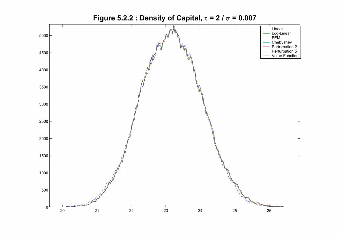
20 21 22 23 24 25 260

500

1000

1500

2000

2500

3000

3500

4000

4500

5000

Figure 5.2.2 : Density of Capital, τ = 2 / σ = 0.007LinearLog-LinearFEMChebyshevPerturbation 2Perturbation 5Value Function

0.295 0.3 0.305 0.31 0.315 0.32 0.3250

1000

2000

3000

4000

5000

6000

7000

Figure 5.2.3 : Density of Labor, τ = 2 / σ = 0.007LinearLog-LinearFEMChebyshevPerturbation 2Perturbation 5Value Function

1.15 1.2 1.25 1.3 1.35 1.40

1000

2000

3000

4000

5000

6000

Figure 5.2.4 : Density of Consumption, τ = 2 / σ = 0.007LinearLog-LinearFEMChebyshevPerturbation 2Perturbation 5Value Function

50 100 150 200 250 300 350 400 450 500

1.65

1.7

1.75

1.8

1.85

1.9

Figure 5.2.5: Time Series for Output, τ = 2 / σ = 0.007LinearLog-LinearFEMChebyshevPerturbation 2Perturbation 5Value Function

50 100 150 200 250 300 350 400 450 500

22.5

23

23.5

24

24.5

Figure 5.2.6: Time Series for Capital, τ = 2 / σ = 0.007LinearLog-LinearFEMChebyshevPerturbation 2Perturbation 5Value Function

0.5 1 1.5 2 2.5 3 3.5 4 4.5 5 5.5 60

1000

2000

3000

4000

5000

6000

7000

8000

Figure 5.2.7 : Density of Output, τ = 50 / σ = 0.035LinearLog-LinearFEMChebyshevPerturbation 2Perturbation 5Perturbation 2(log)Value Function

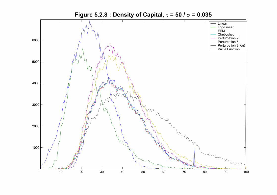
10 20 30 40 50 60 70 80 90 1000

1000

2000

3000

4000

5000

6000

Figure 5.2.8 : Density of Capital, τ = 50 / σ = 0.035LinearLog-LinearFEMChebyshevPerturbation 2Perturbation 5Perturbation 2(log)Value Function

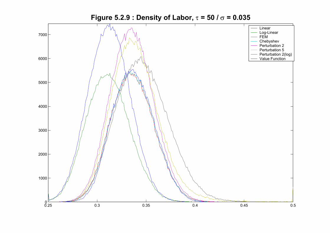
0.25 0.3 0.35 0.4 0.45 0.50

1000

2000

3000

4000

5000

6000

7000

Figure 5.2.9 : Density of Labor, τ = 50 / σ = 0.035LinearLog-LinearFEMChebyshevPerturbation 2Perturbation 5Perturbation 2(log)Value Function

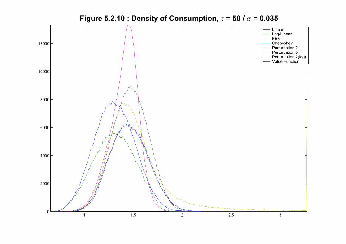
1 1.5 2 2.5 30

2000

4000

6000

8000

10000

12000

Figure 5.2.10 : Density of Consumption, τ = 50 / σ = 0.035LinearLog-LinearFEMChebyshevPerturbation 2Perturbation 5Perturbation 2(log)Value Function

50 100 150 200 250 300 350 400 450 5000.5

1

1.5

2

2.5

3

Figure 5.2.11 : Time Series for Output, τ = 50 / σ = 0.035

LinearLog-LinearFEMChebyshevPerturbation 2Perturbation 5Perturbation 2(log)Value Function

50 100 150 200 250 300 350 400 450 5000

5

10

15

20

25

30

35

40

45

Figure 5.2.12 : Time Series for Capital, τ = 50 / σ = 0.035

LinearLog-LinearFEMChebyshevPerturbation 2Perturbation 5Perturbation 2(log)Value Function

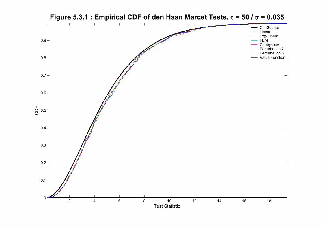
2 4 6 8 10 12 14 16 180

0.1

0.2

0.3

0.4

0.5

0.6

0.7

0.8

0.9

Figure 5.3.1 : Empirical CDF of den Haan Marcet Tests, τ = 50 / σ = 0.035

Test Statistic

CD

F

Chi-SquareLinearLog-LinearFEMChebyshevPerturbation 2Perturbation 5Value Function

0 5 10 15 20 250

0.1

0.2

0.3

0.4

0.5

0.6

0.7

0.8

0.9

Figure 5.3.2 : Empirical CDF of den Haan Marcet Tests, τ = 50 / σ = 0.035

Test Statistic

CD

F

Chi-SquareLinearLog-LinearFEMChebyshevPerturbation 2Perturbation 5Perturbation 2(log)Value Function

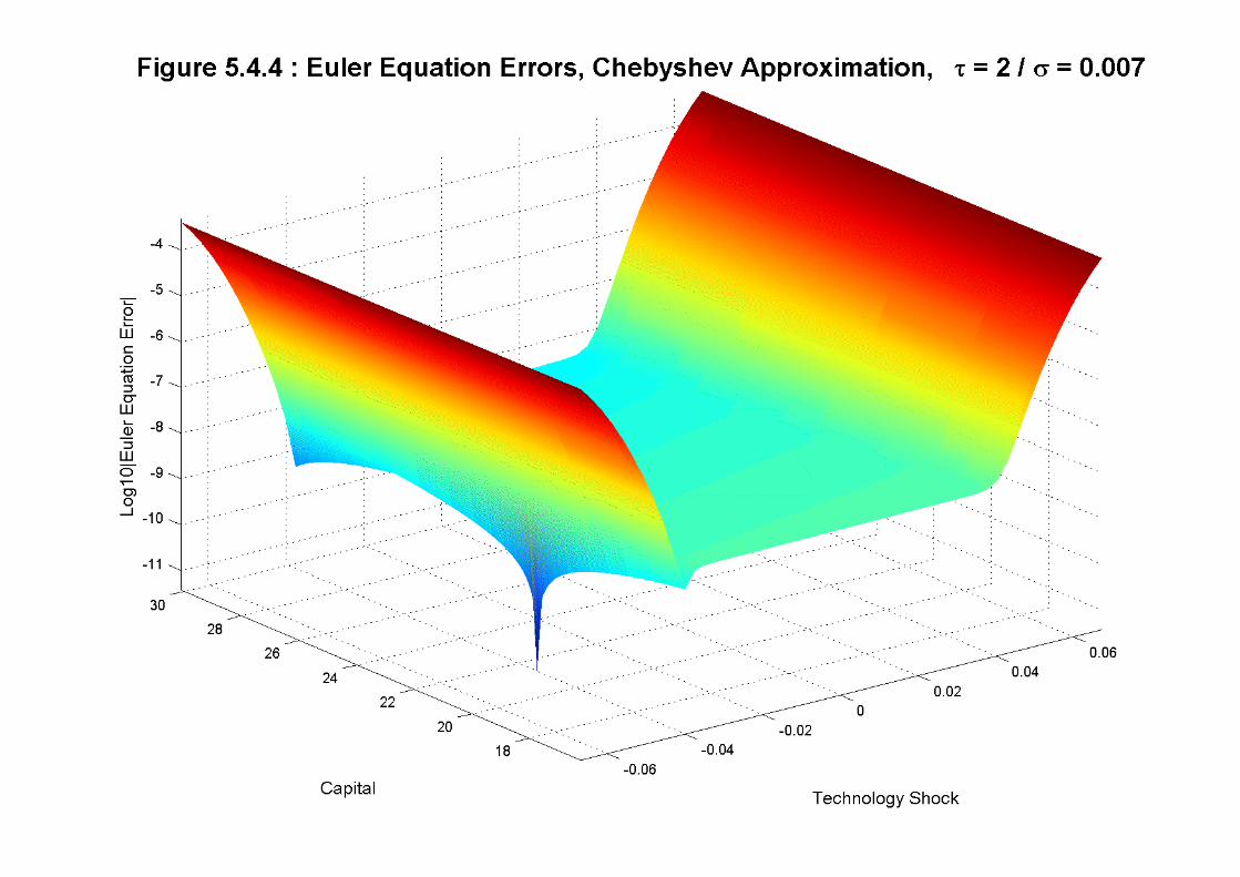
18 20 22 24 26 28 30

-9

-8

-7

-6

-5

-4

-3

Figure 5.4.8 : Euler Equation Errors at z = 0, τ = 2 / σ = 0.007

Capital

Log1

0|E

uler

Equ

atio

n E

rror

|

LinearLog-LinearFEMChebyshevPerturbation 2Perturbation 5Value Function

18 20 22 24 26 28 30

0

2

4

6

8

10

12

14

16

18x 10-4 Figure 5.4.9 : Euler Equation Errors at z = 0, τ = 2 / σ = 0.007

Capital

Eul

er E

quat

ion

Err

or

LinearLog-LinearFEMChebyshevPerturbation 2Perturbation 5Value Function

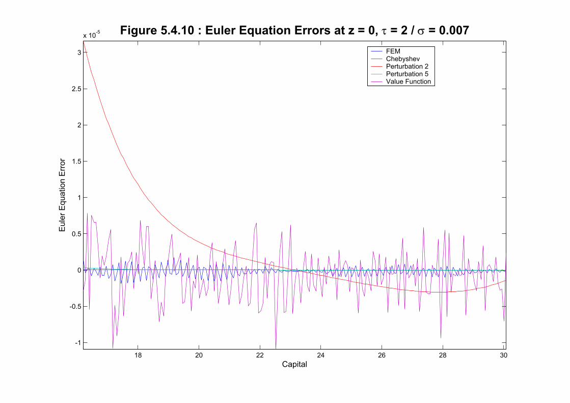
18 20 22 24 26 28 30

-1

-0.5

0

0.5

1

1.5

2

2.5

3

x 10-5 Figure 5.4.10 : Euler Equation Errors at z = 0, τ = 2 / σ = 0.007

Capital

Eul

er E

quat

ion

Err

orFEMChebyshevPerturbation 2Perturbation 5Value Function

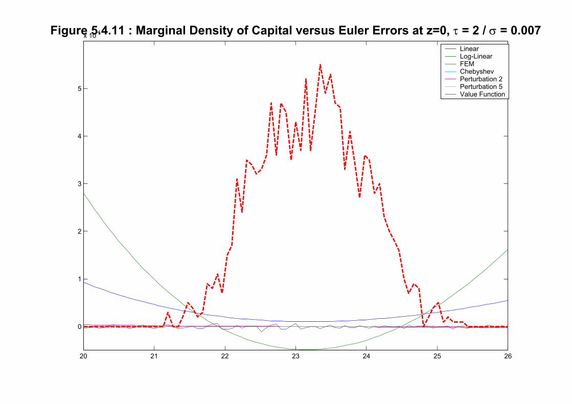
20 21 22 23 24 25 26

0

1

2

3

4

5

x 10-4Figure 5.4.11 : Marginal Density of Capital versus Euler Errors at z=0, τ = 2 / σ = 0.007LinearLog-LinearFEMChebyshevPerturbation 2Perturbation 5Value Function

25 30 35 40 45 50

-6.5

-6

-5.5

-5

-4.5

-4

-3.5

-3

Figure 5.4.20 : Euler Equation Errors at z = 0, τ = 50 / σ = 0.035

Capital

Log1

0|E

uler

Equ

atio

n E

rror

|

LinearLog-LinearFEMChebyshevPerturbation 2Perturbation 5Perturbation 2(log)Value Function