Thesis no: MEE10:70

Comparative Study of WIMAX and

LTE Uplink Using SDCMA and

LSCMA

Jaswini Reddy Potuganuma

This thesis is presented as part of the Degree of

Master of Science in Electrical Engineering

Blekinge Institute of Technology

June 2010

Blekinge Institute of Technology Virginia Polytechnic Institute and State University

School of Engineering Bradley Department of Electrical and computer

Department of Electrical Engineering Engineering

Internal Supervisor: Dr. Jörgen Nordberg External Supervisor: Dr.Tamal Bose

2

ABSTRACT

Blind equalizers are widely used in wireless communications for minimizing Inter Symbol

Interference (ISI). The Constant Modulus Algorithm (CMA) is one of the popular blind

equalizers used in broad band applications. This master‘s thesis investigates the Steepest Descent

Constant Modulus Algorithm (SDCMA) i.e. CMA (1, 2) and CMA (2, 2), and the Least Square

Constant Modulus Algorithm (LSCMA) in the time domain and frequency domain. A

Fractionally Spaced Equalizer (FSE) compares them using convergence and Bit Error Rate

(BER) vs. Signal to Noise Ratio (SNR). The second part of the thesis compares the performance

of WiMax OFDM PHY (Orthogonal Frequency Division Multiplexing Physical layer) and

Single Carrier LTE (Long Term Evolution) uplink PHY using FD-SDCMA (Frequency Domain-

SDCMA) and FD-LSCMA (Frequency Domain- LSCMA). WiMax and Single Carrier LTE

uplink are compared using BER vs. SNR. All simulations are done in MATLAB.

3

ACKNOWLEDGMENT

This master‘s thesis will help me achieve my dream of obtaining the MSc degree in signal

processing. I would like to thank and express a deep sense of gratitude and respect to my

external supervisor and examiner Dr. Tamal Bose, Professor, Department of Engineering,

Virginia Tech, USA, for his able guidance and cooperation throughout my work on the project. I

am highly grateful to him for providing all the facilities needed for completion of this work.

I would like to offer hearty thanks to Bei Xie, PhD student, Virginia Tech, USA, for the untiring

inspiration and motivation I needed to complete this thesis.

I am very thankful and grateful to my internal supervisor, Dr. Jörgen Nordberg, Department of

Electrical Engineering, Blekinge Tekniska Högskola, Sweden, for his encouragement and

cooperation toward the successful completeion of my master‘s thesis at Virgina Tech, USA.

Jaswini Reddy Potuganuma

August 2010

4

TABLE OF CONTENTS

Abstract...........................................................................................................................................2

Acknowledgement...........................................................................................................................3

Contents ..........................................................................................................................................4

List of figures...................................................................................................................................8

Abbreviations.................................................................................................................................10

Chapter 1: Introduction

1.1 Motivation..............................................................................................................................13

1.2 Objective................................................................................................................................14

1.3 Organization ofThesis............................................................................................................15

1.4 Published related works...........................................................................................................15

Chapter 2: Comparison of SDCMA and LSCMA in time domain

2.1 Overview of CMA .................................................................................................................16

2.2 SDCMA derivation..................................................................................................................16

2.3 Overview of LSCMA...............................................................................................................17

2.4 Blind equalizer ........................................................................................................................20

2.4.1 Description............................................................................................................................20

2.5 Algorithm of CMA (1,2), CMA(2,2) and LSCMA using blind equalizer...............................21

2.6 Comparison of SDCMA and LSCMA using blind equalizer..................................................22

5

2.6.1 Output SDCMA and LSCMA using blind equalizer............................................................22

2.6.2 Comparing SDCMA and LSCMA using convergence.........................................................23

2.6.3 Comparing SDCMA and LSCMA using BER vs. SNR......................................................23

2.7 Fractionally Spaced Equalizer (FSE).......................................................................................24

2.7.1 Description............................................................................................................................25

2.8 Algorithm for CMA(1,2), CMA(2,2) and LSCMA using FSE...............................................26

2.9 Comparison of SDCMA and LSCMA using FSE...................................................................27

2.9.1 Outputs of SDCMA and LSCMA using FSE.......................................................................27

2.9.2 Comparing SDCMA and LSCMA using convergence.........................................................28

2.9.3 Comparing SDCMA and LSCMA using BER vs. SNR......................................................29

Chapter 3: Comparison of FD-SDCMA and FD-LSCMA

3.1 Introduction.............................................................................................................................30

3.2 Block diagram of FDCMA using blind equalizer....................................................................30

3.2.1 Description............................................................................................................................31

3.3 Algorithm of FDCMA using blind equalizer...........................................................................32

3.4 Comparison of FDCMA using blind equalizer........................................................................32

3.4.1 Outputs of FD-SDCMA and FD-LSCMA using blind equalizer........................................32

3.4.2 Comparing FD-SDCMA and FD-LSCMA using convergence...........................................33

3.4.3 Comparing FD-SDCMA and FD-LSCMA using BER vs. SNR........................................34

3.5 Block diagram of FDCMA using FSE....................................................................................36

3.5.1 Description............................................................................................................................36

3.6 Algorithm of FDCMA using FSE............................................................................................37

3.7 Comparison of FD-SDCMA and FD-LSCMA using FSE......................................................38

6

3.7.1 Outputs of FD-SDCMA and FD-LSCMA using FSE.........................................................38

3.7.2 Comparing FD-SDCMA and FD-LSCMA using convergence............................................38

3.7.3 Comparing FD-SDCMA and FD-LSCMA using BER vs. SNR.........................................40

Chapter 4: Design and Implementation of CMA in WiMax and LTE uplink

4.1 Orthogonal Frequency Division Multiplexing (OFDM)..........................................................42

4.2 Advantages and disadvantages of OFDM...............................................................................43

4.2.1 Advantages............................................................................................................................43

4.2.2 Disadvantages.......................................................................................................................43

4.3 Overview of WiMax................................................................................................................44

4.4 WiMax physical layer..............................................................................................................45

4.5 Features of WiMax..................................................................................................................45

4.6 Advantages and disadvantages of WiMax..............................................................................46

4.6.1 Advantages............................................................................................................................46

4.6.2 Disadvantages.......................................................................................................................46

4.7 System model...........................................................................................................................47

4.7.1 Transmitter module...............................................................................................................47

4.7.2 Receiver module...................................................................................................................51

4.8 Simulation results.....................................................................................................................52

4.9 Single carrier LTE uplink........................................................................................................53

4.9.1 Introduction..........................................................................................................................53

4.10 System model.........................................................................................................................54

4.11 Comparion of SDCMA and LSCMA using SCFDM LTE uplink.........................................56

7

4.12 Comparison of SDCMA and LSCMA using WiMax OFDM PHY and SC-FDM LTE uplink

PHY ....................................................................................................................... .....................56

Chapter 5: Conclusions

Conclusion.................................................................................................................................... .57

References......................................................................................................................................58

8

List of Figures

Fig.2.1 Block diagram of blind equalizer.

Fig.2.2 Outputs of SDCMA and LSCMA using blind equalizer.

Fig.2.3 Convergence of SDCMA and LSCMA using blind equalizer.

Fig.2.4 Comparison of SDCMA and LSCMA using blind equalizer.

Fig.2.5 Block diagram of multi channel fractionally spaced equalizer.

Fig.2.6 Outputs of SDCMA and LSCMA using FSE.

Fig.2.7 Convergence of SDCMA and LSCMA using FSE in time domain.

Fig 2.8 Comparison of SDCMA and LSCMA using BER vs. SNR in FSE time domain.

Fig.2.9 Comparison of SDCMA and LSCMA using FSE and blind equalizer in time domain.

Fig. 3.1 Block diagram of FDCMA using blind equalizer.

Fig. 3.2 Outputs of FD-LSCMA and FD-SDCMA using blind equalizer.

Fig. 3.3 Convergence of FD-SDCMA and FD-LSCMA using blind equalizer.

Fig. 3.4 Comparison of SDCMA and LSCMA in frequency domain using BER vs. SNR.

Fig. 3.5 Block diagram of FDCMA using FSE.

Fig. 3.7 Outputs of FD-SDCMA and FD-LSCMA using FSE.

Fig. 3.8 Comparison of convergence of FD-SDCMA and FD-LSCMA using FSE.

Fig. 3.9 Comparison of FD-SDCMA and FD-LSCMA using BER vs. SNR.

Fig. 4.1 Frequency Division Multiplexing (FDM). Spacing is put between two adjacent sub

carriers.

Fig. 4.2 Orthogonal Frequency Division Multiplexing (OFDM). Sub carriers are closely spaced

until overlap.

Fig. 4.3 Block diagram of 802.16e OFDM PHY.

9

Fig. 4.4 I and Q axis outputs of BPSK (1,1), QAM (1,2), 16 QAM (2,1) and 64 QAM (2,2).

Fig. 4.5 Block diagram OFDM modulator.

Fig. 4.6 Block diagram of OFDM demodulator.

Fig. 4.7 Comparison of FD-SDCMA and FD-LSCMA using WiMax OFDM PHY.

Fig. 4.8 Block diagram of SC-FDM using LTE uplink PHY.

Fig. 4.9 Comparison of FD-SDCMA and FD-LSCMA using SC-FDM LTE uplink PH.

Fig. 4.10 Comparison of SDCMA and LSCMA using WiMax OFDM PHY and SC-FDM uplink

PHY.

10

Abbreviations

ADC—Analog to Digital Converter

AWGN—Additive White Gaussian Noise

BER—Bit Error Rate

CDS—Channel Dependent Scheduling

CMA—Constant Modulus Algorithm

CP—Cyclic Prefix

DFDMA—Distributed FDMA

DFT—Discrete Fourier Transform

FDCMA—Frequency Domain Constant Modulus Algorithm

FD-LSCMA—Frequency Domain Least Square Constant Modulus Algorithm

FDM—Frequency Division Multiplexing

FDMA—Frequency Division Multiple Access

FD-SDCMA—Frequency Domain Steepest Descent Constant Modulus Algorithm

FEC—Forward Error Correction

FFT—Fast Fourier Transform

FSE—Fractionally Spaced Equalizer

IBI—Inter Block Interference

ICI—Inter Carrier Interference

IEEE—Institute of Electrical and Electronic Engineers

IFFT—Inverse Fast Fourier Transform

11

IFDMA—Interleaved FDMA

ISI—Inter Symbol Interference

LFDMA—Localized FDMA

LSCMA—Least Square Constant Modulus Algorithm

LTE—Long Term Evolution

MIMO—Multiple Input and Multiple Output

MSE—Mean Square Error

OFDM—Orthogonal Frequency Division Multiplexing

OFDMA—Orthogonal Frequency Division Multiple Access

PAN—Personal Area Networks

PAPR—Peak to Average Power Ratio

PHY—PHYsical layer

QAM—Quadrature Amplitude Modulation

QPSK—Quadrature Phase Shift Keying

SC—Single Carrier

SC-FDM—Single Carrier Frequency Domain Modulation

SC-FDMA—Single Carrier Frequency Division Multiple Access

SDCMA—Steepest descent Constant Modulus Algorithm

SNR—Signal to Noise Ratio

SRC—Static Resource Allocation

WAN—Wireless Area Networks

WiMax—Worldwide Interoperability for Microwave Access

12

WLAN—Wireless Local Area Networks

WMAN—Wireless Metropolitan Access Network

3GPP—3rd Generation Partnership Project

13

CHAPTER 1

INTRODUCTION 1.1 Motivation

Broadband and mobile services are expanding rapidly. Due to this, Broadband Wireless Access

(BWA) networks have gained remarkable importance in recent years. Depending on the network,

a large number of wireless technologies like LAN, PAN, WLAN, and WMAN are used in

today‘s world. A new standard is developed by IEEE called 802.16 also called Worldwide

Interoperability for Microwave Access (WiMax) is introduced to fulfill all these requirements:

networks having high data transfer, variable transfer rate, high SNR, mobility and compatibility

between the same networks and different technologies.

WiMax has a flexible network architecture, enables mobile convergence, and has fixed

broadband networks. WiMax introduced single carrier PHY and OFDM PHY. 802.16e OFDM

PHY is designed to overcome the effects of multi path propagation by performing frequency

domain equalization [3].

The demand for high data transfer is growing rapidly in mobile communications. To meet

this demand, the 3rd Generation Partnership Project (3GPP) has developed technical

specifications called Long Term Evolution (LTE) [4], [5]. The main objective of LTE is to

develop high data transfer and packet optimized radio access technology for 3GPP [4], [5].

Single Carrier Frequency Division Multiplexing (SC-FDM) is selected for LTE uplink to reduce

Peak to Average Power Ratio (PAPR). The performance of SC-FDM is similar to that of OFDM

[6].

CMA is one of the famous blind equalizers used in communications. It has less

computational complexity, is simple and easy to implement, and has non negative cost function.

This thesis compares LSCMA and SDCMA in the time and frequency domains using a

14

blind equalizer and FSE. This thesis attempts to compare FDSDCMA and FDLSCMA by

implementing it, with 802.16e OFDM PHY and Single Carrier Frequency Division Multiplexing

(SCFDM) formats by employing cyclic prefixes and LTE uplink using SC-FDM in the physical

layer.

1.2 Objective

The main objective of this project is to compare the performance of LSCMA and SDCMA in the

time domain and the frequency domain by using a blind equalizer and FSE. Comparing the

performance of LSCMA and SDCMA in the frequency domain using IEEE 802.16e OFDM

PHY, and LTE uplink using SC-FDM in PHY.

The objective of the project can be summarized as follows.

Step 1: Implementation of the time domain and the frequency domain of LSCMA and SDCMA

using a blind equalizer and FSE.

Step 2: Comparing them using convergence, BER vs. SNR.

Step 3: Design IEEE 802.16e OFDM PHY in MATLAB.

Step 4: Compare the performance of the frequency domain of LSCMA and SDCMA using IEEE

802.16e OFDM PHY

Step 5: Implement the frequency domain of LSCMA and SDCMA using single carrier

modulation formats employing periodic cyclic prefixes and the LTE uplink using SC-FDM in

PHY.

1.3 Organization of the thesis

The thesis is organized as follows.

Chapter 2

This chapter deals with an overview of CMA, derivation of SDCMA i.e. CMA 12 and CMA 22,

15

and implementation of SDCMA and LSCMA using a blind equalizer and FSE in the time

domain and comparing them using convergence, BER vs. SNR.

Chapter 3

This chapter deals with an overview of the frequency domain CMA, and implementation of

SDCMA and LSCMA using a blind equalizer and FSE in the frequency domain and comparing

them using convergence, BER vs. SNR.

Chapter 4

The chapter covers the background and introduces WiMax and discuss the advantages and

disadvantages of WiMax, provide a brief introduction to the OFDM technique, introduce the

single carrier modulation formats, periodic cyclic prefixes, and LTE uplink PHY, and discuss the

design and implementation and compare the performance of the frequency domain LSCMA and

SDCMA in 802.16e OFDM PHY and SC-FDM LTE uplink using cyclic prefix.

Chapter 5

This chapter includes the conclusions that can be reached by using the useful information

presented in this thesis.

1.4 Published related works

The related works of CMA, WiMax OFDM PHY, and the SC-FDM LTE uplink can be seen in

[1], [7],[8],[9],[10] and [11] ; [2], [3], [12], [13], [14], [23] and [24]; [4], [5] and [6].

16

CHAPTER 2

COMPARISON OF LSCMA AND SDCMA IN THE TIME DOMAIN

2.1 Overview of CMA

ISI is one of the practical problems faced in digital communications. ISI distorts the transmitted

signal due to channel band limiting and multipath signals in the channel. To compensate for ISI

at the receiver side in a communication system, adaptive filters are used. In practice, trained

adaptive filters are not used. For non training signals in communication systems, blind equalizers

are used. The problem with blind equalization is poor convergence compared with the trained

sequence. Steepest descent based algorithms are used for blind equalization. A widely used blind

equalizer is the constant modulus algorithm, which is proposed by Godard [1]. If the constant

modulus property is lost due to noise, one can restore the original signal using CMA.

2.2 SDCMA Derivation[3]

Let x(k) be the distorted input signal at the receiver side in digital communication and W(k) be

the adjustable weight vector. Let J be the positive average of Y(k) that deviates from the unity

modulus condition. Then the filter output is

Y(k)=XT(k)*W(k), (1)

where X(k) is the input data matrix and W(k) is the weight vector

X(k)=[x(k)x(k-1)…x(k-N+1)]T,

W(k)=[w0(k)…wN-1(k)]T.

The main objective of the adaptive filter is to regain the original signal that is transmitted. This

can be obtained by changing the weight vectors to minimize J and make the filter output close

towards unit length. The mathematical equation of J for CMA(2,2) is

J = E{[|y(k)|2 - 1]

2}, (2)

17

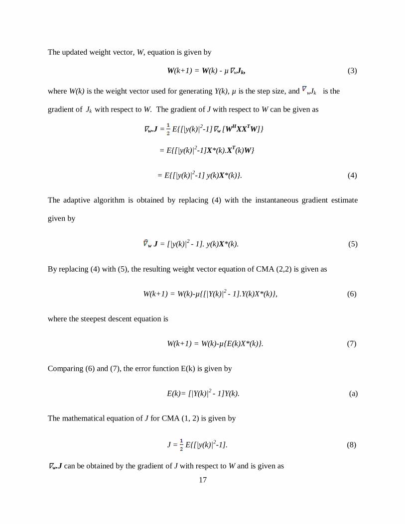
The updated weight vector, W, equation is given by

W(k+1) = W(k) - µ∇wJk, (3)

where W(k) is the weight vector used for generating Y(k), µ is the step size, and wJk is the

gradient of Jk with respect to W. The gradient of J with respect to W can be given as

∇w.J = E{[|y(k)|2-1]∇w [W

HXX

TW]}

= E{[|y(k)|2-1]X*(k).X

T(k)W}

= E{[|y(k)|2-1] y(k)X*(k)}. (4)

The adaptive algorithm is obtained by replacing (4) with the instantaneous gradient estimate

given by

w J = [|y(k)|2 - 1]. y(k)X*(k). (5)

By replacing (4) with (5), the resulting weight vector equation of CMA (2,2) is given as

W(k+1) = W(k)-µ{[|Y(k)|2 - 1].Y(k)X*(k)}, (6)

where the steepest descent equation is

W(k+1) = W(k)-µ{E(k)X*(k)}. (7)

Comparing (6) and (7), the error function E(k) is given by

E(k)= [|Y(k)|2 - 1]Y(k). (a)

The mathematical equation of J for CMA (1, 2) is given by

J = E{[|y(k)|2-1]. (8)

∇w.J can be obtained by the gradient of J with respect to W and is given as

18

∇w.J =E{[|Y(k)| -1]∇w.[WHX]}

= E{[|Y(k)| -1]X*(k)}

= E{[|Y(k)| -1]X*(k)}. (9)

and

Y(k)/|Y(k)| =1. (10)

Substituting (10) in (9), the gradient of Jk is given as

wJk= E{[|Y(k)| - Y(k)/|Y(k)|]X*(k)}. (11)

The approximate gradient for (10) is given as

w J = [|Y(k)| - Y(k)/|Y(k)|]X*(k). (12)

Therefore CMA (1, 2) can be obtained by substituting (12) in (3)

W(k+1)=W(k)-µ[|Y(k)| - Y(k)/|Y(k)|]X*(k). (13)

Comparing (13) and (7), the error function is given by

E(k)= [|Y(k)| - Y(k)/|Y(k)|]. (b)

2.3 Overview of LSCMA

The main drawback of CMA is slow convergence. To overcome this, LSCMA is proposed by

Agee [7]. LSCMA can be obtained by integrating the Least Square Estimator (LSE) and

Constant Modulus (CM). It rapidly converges and is stable for linearly independent stable signals

[7].

LSCMA is developed by extension of the non linear least square Gauss‘s method to the complex

argument cost function [7]. The derivation of LSCMA is as follows [7]. The cost function F(w)

is given by

F(w) = n2(w) = || Ф(w) || . (14)

19

where Ø(w) is the error signal.

The (14) has partial Taylor series with sum of squares is shown as

F (w+∆) || Ф (w )+JT(w) ∆ || ,

(15)

where

J(w) = [∇Ø1(w), ∇Ø2(w),…. ∇ØN(w)]. (16)

The weight vectors in the Gauss‘s method are updated as

wk+1 = wk-[J(wk)JT(wk)]

-1J(wk) Ф(wk). (17)

J JT is a semi definite positive approximation of J. The sum of square components of the

complex Taylor series are given by [9]

F (w+∆) || Ф (w )+J+(w) ∆ || . (18)

where ∆ minimizes the sum of squares and J+ indicates the conjugate transpose of J . The

optimization of (17) is

wk+1 = wk-[J(wk) J+((wk)]

-1J(wk) Ф(wk). (19)

The least square constant modulus algorithm is derived from (19) by applying the constant

modulus cost function.

W(k) = 2 . (20)

Substitute y(n) = wT

x(n) in (20), the weight vector equation is given as

W(k)= || [ |xT(k)w| -1 ] || . (21)

20

Substituting (21) in (19), the resulting least square constant modulus algorithm is given by

wK+1 = wk - (XXT)

-1X*( yk-δk )

= (XXT)

-1X*( δk ). (22)

where X is input data and yk and δk are output data and complex output data is limited

X = [x(1),x(2),…..x(N)],

yk = [yk(n)] = XTwk and

δk = [δk(n)] = |yk(n)/|yk(n)||.

Comparing (22) with (7), the error function is given as

E(k)= (XXT)

-1(yk-δk ). (c)

2.4 Blind Equalizer

In communication systems, the removal of ISI plays a prominent role in regaining the desired

signal at the receiver side. Adaptive filters used in real time applications donot have training

signals i.e., the desired signal is unknown. This can be demonstrated by using blind equalization,

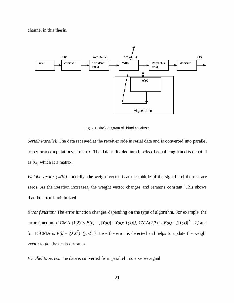
which helps to minimize ISI. One of the famous blind equalizers is CMA. The block diagram of

the blind equalizer is shown in Fig.2.1 [10].

2.4.1. Description

Input: The signal is any type i.e., an audio, video, or data signal. It is represented as x(t).

Channel: The channel is the medium in which the input signal is transmitted, and it may be

wired or wireless. Noise is added to the input signal in the channel. Channel used is a stationary

21

channel in this thesis.

Fig. 2.1 Block diagram of blind equalizer.

Serial/ Parallel: The data received at the receiver side is serial data and is converted into parallel

to perform computations in matrix. The data is divided into blocks of equal length and is denoted

as Xk, which is a matrix.

Weight Vector (w(k)): Initially, the weight vector is at the middle of the signal and the rest are

zeros. As the iteration increases, the weight vector changes and remains constant. This shows

that the error is minimized.

Error function: The error function changes depending on the type of algorithm. For example, the

error function of CMA (1,2) is E(k)= [|Y(k)| - Y(k)/|Y(k)|], CMA(2,2) is E(k)= [|Y(k)|

2 – 1] and

for LSCMA is E(k)= (XXT)

-1(yk-δk ). Here the error is detected and helps to update the weight

vector to get the desired results.

Parallel to series:The data is converted from parallel into a series signal.

22

Decision: The serial signal is sent to a decision where the desired signal is obtained.

2.5 Algorithm for CMA (1,2), CMA(2,2) and LSCMA using blind equalizer

Step 1: Initialize the input signal, block length, signal length, error signal, step size, and weight

vectors.

Step 2: The received signal consists of the input signal and noise. The received series signal is

converted into parallel signals whose length equals the block length.

Step 3: Takes a loop and iteration and continues to the length of the received signal.

Step 4: Calculate the error signals for CMA(1,2), CMA(2,2), and LSCMA.

Step 5: Calculate the weight vectors for CMA(1,2), CMA(2,2), and LSCMA.

Step 6: End of loop.

Step 7: Calculate the output and convergence and plot the results.

2.6 Comparison of SDCMA and LSCMA using blind equalizer

The comparison of SDCMA and LSCMA is done by taking different parameters like the

received signal, convergence, and BER vs. SNR. For the received signal and convergence, the

step size is 0.0001 for SDCMA, the smoothing length is 16, SNR is 14, and the number of

samples is 5000. The channel is a multipath channel and AWGN is also included. The channel

equation used in this example is

h(n)= -0.25δ(n)+0.085δ(n-1)+1.2δ(n-2)-0.02δ(n-3)+0.25δ(n-4)-0.5δ(n-5).

23

2.6.1 Outputs of SDCMA and LSCMA using blind equalizer

Fig. 2.2 shows the transmitted signal, which is QAM or QPSK, at the transmitted side. It is

received at the receiver side where multipath signals and AWGN are included in the received

signal. CMA (1,2), CMA(2,2), and LSCMA algorithm outputs are shown in Fig. 2.2 using a

single channel.

2.6.2 Comparison of SDCMA and LSCMA using convergence

The convergence is used to reach the equilibrium state. Fig. 2.3 shows the convergence of

CMA(1,2), CMA(2,2), and LSCMA. From Fig. 2.3, it can be seen that the convergence of

LSCMA is faster compared to that of CMA 2-2 and CMA 1-2.

Fig. 2.2 Outputs of SDCMA and LSCMA using blind equalizer.

24

Fig. 2.3 Convergence of SDCMA and LSCMA using blind equalizer.

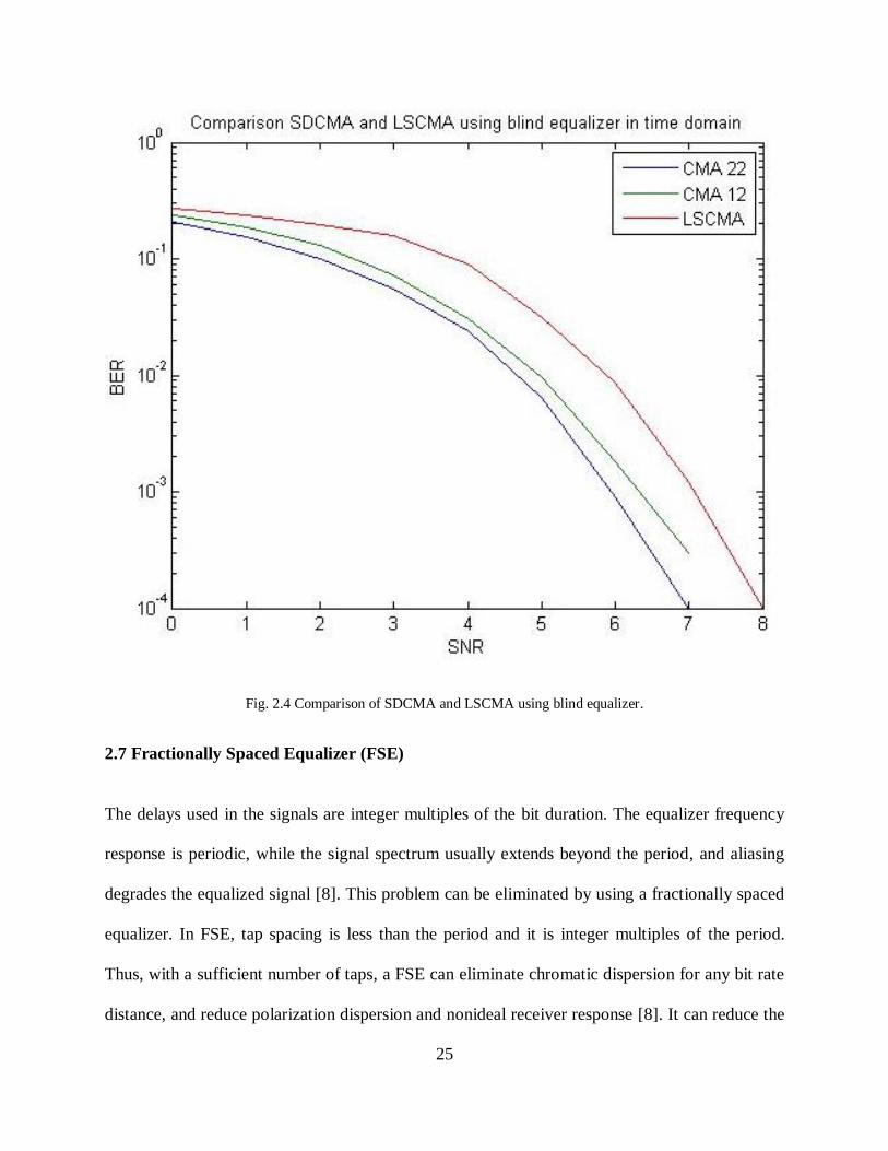
2.6.3 Comparing SDCMA and LSCMA using BER vs. SNR

For different values of SNR, the BER varies. This can be observed in Fig. 2.4 for SDCMA and

LSCMA. From Fig. 2.4., it is clear that the SNR of CMA 22 is better when compared to the

other two algorithms. The LSCMA has poor BER with repect to SNR. This is due to instability

in the LSCMA‘s error though it convergence fast compared to SDCMA, and minimum errror of

LSCMA is greater than SDCMA .

25

Fig. 2.4 Comparison of SDCMA and LSCMA using blind equalizer.

2.7 Fractionally Spaced Equalizer (FSE)

The delays used in the signals are integer multiples of the bit duration. The equalizer frequency

response is periodic, while the signal spectrum usually extends beyond the period, and aliasing

degrades the equalized signal [8]. This problem can be eliminated by using a fractionally spaced

equalizer. In FSE, tap spacing is less than the period and it is integer multiples of the period.

Thus, with a sufficient number of taps, a FSE can eliminate chromatic dispersion for any bit rate

distance, and reduce polarization dispersion and nonideal receiver response [8]. It can reduce the

26

sensitivity of the detector to timing offset. To perform time and phase recovery, fractionally

spaced equalizers are used in digital communications [8]. To get detailed information regarding

the channel, the over sampling of the received signal is done by the fractional spaced equalizer

[9]. FSE is mainly used for combating ISI due to its improved performance. It is used to estimate

the equalizer directly and it has global convergence. FSE is classified into two types: multi rate

FSE and multi channel or multi path FSE.

Multirate FSE: Multirate FSE is a single channel FSE. If the length of the input signal s(n) is N,

T is the period of the signal, and the tap spacing is T/2, then the input signal used for

transmission will have either a multiple of 2N or 2N+1 elements. They are transmitted after

upsampling.

Multipath FSE: In multipath FSE, the channel is divided into sub-channels. For example, if it is a

two path FSE, and the channel length is L, then the elements in multiples of 2L in the channel

are kept in one sub-channel and elements in multiples of 2L+1 are kept in another sub-channel.

The block diagram of multi channel FSE is shown in Fig.2.5.

2.7.1 Description

The input signal Xn is at the transmitter side, and is transmitted to different sub-channels. The

sub-channels are of many types; they may be optical channels, wired channels, or wireless

channels. The signal transmitted by this channel is a combination of the multi path signal and

noise. At the receiver side, the receiver doesnot know the real input signal, so equalizers are

used.

27

Fig. 2.5 Block diagram of multi channel fractionally spaced equalizer.

The weight vectors are initialised.The signal received at the equalizer is divided into blocks of

the same length. The weight vector varies depending on the error. As the iteration increases, the

error tends to zeros or minimum values. Here, the error function depends on the type of CMA

used. For example, the cost function of CMA (1,2) is E(k)= [|Y(k)| - Y(k)/|Y(k)|], CMA(2,2) is

E(k)= [|Y(k)|2 – 1] and for LSCMA is E(k)= (XX

T)

-1(yk-δk ) .

2.8 Algorithm for CMA (1,2), CMA(2,2) and LSCMA using FSE

Step 1: Initialize the input signal, block length, signal length, error signal, step size, weight

vectors, and number of sub channels.

Step 2: Add noise to the input signal and create multipath signals in each sub channel and

convert the serial to a parallel signal whose length is equal to the block length.

28

Step 3: Calculate the error signals for CMA(1,2), CMA(2,2), and LSCMA.

Step 4: Calculate the weight vectors for CMA(1,2), CMA(2,2), and LSCMA.

Step 5: Step 3 and Step 4 must be repeated until they equal the length of the signal

Step 6: Calculate the output and convergence and plot the results.

2.9 Comparison of SDCMA and LSCMA using FSE

SDCMA and LSCMA is compared by using convergence and BER vs. SNR

2.9.1 Outputs of SDCMA and LSCMA using FSE

The output is obtained by sending the QAM signal through sub-channels and is shown in Fig.

2.6. The received signal consists of the input signal and noise.

Fig. 2.6 Outputs of SDCMA and LSCMA using FSE.

2.9.2 Comparison of SDCMA and LSCMA using convergence

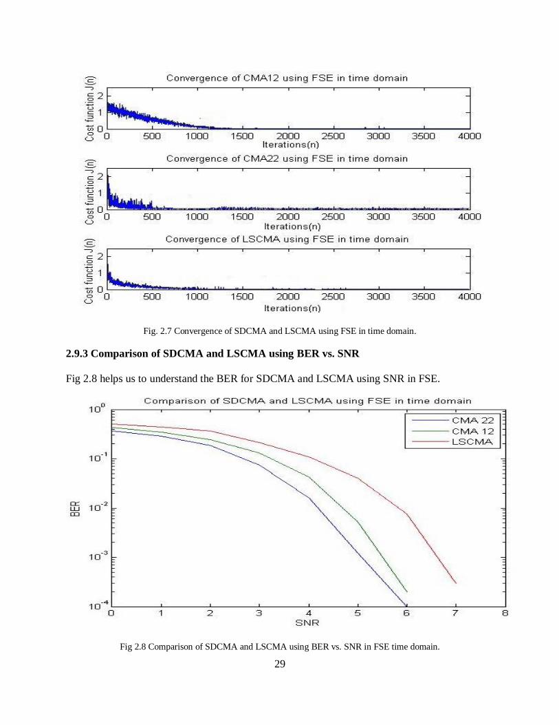
The convergence of SDCMA and LSCMA is shown Fig. 2.7.

29

Fig. 2.7 Convergence of SDCMA and LSCMA using FSE in time domain.

2.9.3 Comparison of SDCMA and LSCMA using BER vs. SNR

Fig 2.8 helps us to understand the BER for SDCMA and LSCMA using SNR in FSE.

Fig 2.8 Comparison of SDCMA and LSCMA using BER vs. SNR in FSE time domain.

30

From Fig. 2.8, it is evident that SDCMA has better BER performance compared to that of

LSCMA using a Fractionally Spaced Equalizer. SDCMA got minimum BER at 6db SNR and for

LSCMA the BER is minimized at 7db. This is due to instability of the optimum error shown in

Fig 2.7 and the minimum error value of LSCMA is greater than CMA 12 and CMA 22.

2.9.4 Comparison of SDCMA and LSCMA using blind eqaulizer and FSE

Fig. 2.9. Comparison of SDCMA and LSCMA using blind equalizer and FSE in time domain.

Fig. 2.4. shows the comparison of SDCMA and LSCMA in the time domain using a blind

equalizer. SDCMA got minimum BER at less SNR compared with LSCMA. Fig. 2.7 shows the

comparison of SDCMA and LSCMA in the time domian using FSE. Here, also, LSCMA got

minimum BER at higher SNR when compared with SDCMA. Fig. 2.9 shows the comparison

between LSCMA and SDCMA in the time domain using a blind equalizer and FSE. SDCMA

using FSE has minimum BER compared to all the other techniques. The convergence of

LSCMA is fast when compared to that of SDCMA in both the blind equalizer and FSE methods.

31

CHAPTER 3

COMPARISON OF FD-SDCMA AND FD-LSCMA

3.1. Introduction

To overcome the computational complexity of CMA in the time domain, the Frequency Domain

Constant Modulus Algorithm (FDCMA) is introduced. In FDCMA, fast linear convolution uses

the DFT overlap save method or the overlap add method. FDCMA is similar to the frequency

domain conventional linear adaptive filter [10]. The error function of CMA is not linear and it is

not straightforward to extend it in the frequency domain. The computational complexity of the

time domain CMA and the frequency domain CMA is N2 and Nlog2 N [11].

3.2 Block diagram of FDCMA using blind equalizer

The block diagram of FDCMA is shown in Fig. 3.1 [11].

Fig. 3.1 Block diagram of FDCMA using blind equalizer.

32

3.2.1 Description

Input signal: The input signal consists of a series of random 1 and -1 bits in complex form. The

input signal is Quadrature Amplitude Modulation (QAM) or Quadrature Phase Shift Keying

(QPSK).

S/P: The serial input signal is converted into parallel by dividing the input signal into blocks of

the same length.

Overlap of previous data: The present block is added after the previous block, which helps to

calculate the linear convolution using the overlap save method.

FFT: Here the input signal block length is doubled since each block consists of the present block

and the previous block. The time domain signal is converted into the frequency domain using the

FFT function in Matlab.

Error function: Calculation of the error function plays an important role in the frequency domain

since it is non linear and the error is calculated in the time domain and converted into the

frequency domain. The input block and the weight vector are converted into the time domain

using the IFFT function. Depending on the type of CMA, the error function varies. For example,

the error function of CMA (1,2) is E(k)= [|Y(k)| - Y(k)/|Y(k)|], CMA(2,2) is E(k)= [|Y(k)|

2 – 1]

and for LSCMA it is E(k)= (XXT)

-1(yk-δk ). After calculating the error, the error is converted into

the frequency domain using the FFT function where the first block is taken as zeros.

Update weight vector: The weight vector is updated and converted into the time domain and the

first block is kept as is, while the second block is converted into zeros.

FFT: The updated weight vector i.e., the first block with calculated values, and the second block

with zeros, is converted into the frequency domain from the time domain.

IFFT: The output signal Y(k) is converted into the time domain by using the IFFT function.

33

Save data: The last block of Y(k) is saved at every iteration

P/S: The parallel blocks are then converted into a series. The desired signal is obtained.

3.3 Algorithm of FDCMA using blind equalizer[11]

FDCMA uses linear convolution with the help of the overlap save method. The following are the

steps needed to calculate FDCMA 2-2, FDCMA 1-2, and FD-LSCMA.

Step 1: Initialize the input signal, signal length, step size, block length, error function, weight

vector, and SNR.

Step 2: Calculate the input signal blocks and the received signal.

Step 3: Add the previous block, as the first block, to the present block, and convert it into the

frequency domain.

Step 4: Add the zeros block to the weight vector as a second block and then convert it into the

frequency domain.

Step 5: Calculate the output vector and then convert it into the time domain.

Step 6: Depending on the type of CMA, the error function varies, and the error is calculated in

the time domain, adding the zero block as the first block. The resulting block is then converted

into the frequency domain.

Step 7: Calculate the weight vector and convert it into the time domain. The first block is saved

and the process is repeated up to the length of the signal.

3.4 Comparison of FDCMA using a blind equalizer

FDCMA is compared to FD-SDCMA and FD-LSCMA using BER vs. SNR convergence and the

outputs from the algorithms.

3.4.1 Output of FD-SDCMA and FD-LSCMA using a blind equalizer

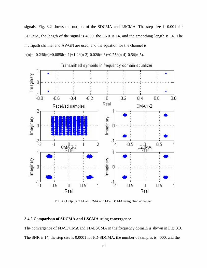
The transmitted signal is a QAM signal and the received signal consists of input and noise

34

signals. Fig. 3.2 shows the outputs of the SDCMA and LSCMA. The step size is 0.001 for

SDCMA, the length of the signal is 4000, the SNR is 14, and the smoothing length is 16. The

multipath channel and AWGN are used, and the equation for the channel is

h(n)= -0.25δ(n)+0.085δ(n-1)+1.2δ(n-2)-0.02δ(n-3)+0.25δ(n-4)-0.5δ(n-5).

Fig. 3.2 Outputs of FD-LSCMA and FD-SDCMA using blind equalizer.

3.4.2 Comparison of SDCMA and LSCMA using convergence

The convergence of FD-SDCMA and FD-LSCMA in the frequency domain is shown in Fig. 3.3.

The SNR is 14, the step size is 0.0001 for FD-SDCMA, the number of samples is 4000, and the

35

smoothing length is 16. The multipath channel uses a FIR filter and AWGN, and the equation for

the channel is h(n)= -0.25δ(n)+0.085δ(n-1)+1.2δ(n-2)-0.02δ(n-3)+0.25δ(n-4)-0.5δ(n-5).

Fig. 3.3 Convergence of FD-SDCMA and FD-LSCMA using blind equalizer.

3.4.3 Comparison of FD-SDCMA and FD-LSCMA using BER vs. SNR

The BER varies with respect to the SNR and also with the algorithm. The comparison of FD-

SDCMA and FD-LSCMA with respect to BER vs. SNR is shown in Fig. 3.4. The minimum

error of LSCMA is greater than SDCMA though LSCMA converges. Due to this, LSCMA has

poor BER performance with respect to SDCMA.

36

Fig. 3.4 Comparison of SDCMA and LSCMA in frequency domain using BER vs. SNR.

3.5 Block diagram of FDCMA using FSE

The block diagram of FDCMA using FSE is shown in Fig. 3.5.

Fig. 3.5 Block diagram of FDCMA using FSE.

37

3.5.1 Description

S/P: The input signal is converted into parallel by dividing the serial signal into blocks of equal

length to perform computations in matrix form.

Overlap of blocks: The blocks are overlapped by adding the previous block as the first block and

the present block as the second block.

FFT: Convert the overlapped blocks into the frequency domain from the time domain.

Error calculation: The error is calculated in the time domain by multiplying the weight vector

and input vector and replacing the second block with zeros. The overlap block is converted into

the frequency domain.

Updating the weight vector: In FSE, there are sub-channels, and the weight vectors are calculated

separately for each sub-channel, as shown in Fig. 3.5. The operation performed in each sub-

channel for calculating the weight vector is similar. The weight vector is updated and converted

into the time domain from the frequency domain. The output is averaged.

FFT: The updated weight vector i.e., the first block with calculated values, and the second block

with zeros, is converted into the frequency domain from the time domain.

IFFT: The output signal Y(k) is converted into the time domain by using the IFFT function.

Save data: The last block of Y(k) is saved in every iteration

P/S: The parallel blocks are then converted into a series. The desired signal is obtained.

3.6 Algorithm of FDCMA using FSE

FDCMA uses linear convolution with the help of the overlap save method. The following are the

steps that are involved to calculate FDCMA 2-2, FDCMA 1-2, and FD-LSCMA.

Step 1: Initialize the input signal, signal length, step size, block length, error function, weight

vector, sub-channels, and SNR.

38

Step 2: Calculate the input signal blocks and the received signal, which consists of AWGN.

Step 3: Add the previous block, as the first block, to the present block, and then convert it into

the frequency domain.

Step 4: Add the zeros block to the weight vector as a second block and then convert it into the

frequency domain.

Step 5: Calculate the averaged output vector and then convert it into the time domain.

Step 6: Depending on the type of CMA, the error function varies, and the error is calculated in

the time domain by adding the zero block as a first block. The resulting block is then converted

into the frequency domain.

Step 7: Calculate the weight vectors for sub-channels and convert them into the time domain.

The first block is saved and the process is repeated up to the length of the signal.

3.7 Comparison of LSCMA and SDCMA using frequency domain FSE

SDCMA and LSCMA is compared by using BER vs. SNR and convergence. In this project, the

step size is 0.0001 for SDCMA, the SNR is 14, and the smoothing length is 16. There are 4 sub-

channels, the signal length is 5000, and they are used for calculating the convergence and the

output of the signal. The recieved signal consists of multipath signals using a FIR filter and

AWGN. The channel used in this example is h(n)=[0.2δ(n)-.09δ(n-1)-.0032δ(n-3);0.092δ(n-1)-

.09δ(n-3);0.8δ(n)-0.1δ(n-2); 0.4δ(n-1)-0.12δ(n-2)+0.2δ(n-3)]

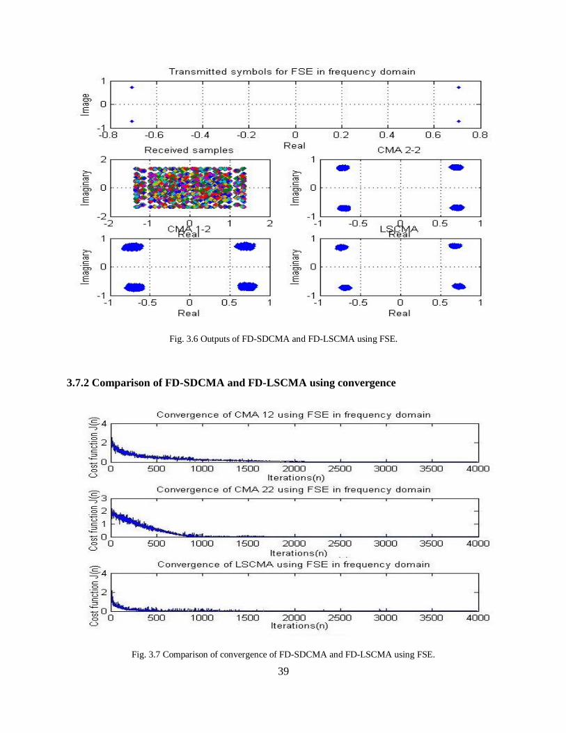
3.7.1 Output of SDCMA and LSCMA using FSE in frequency domain

The input signal is a QAM signal at the receiver side. The received signal consists of multipath

signals from different sub-channels including AWGN. Fig. 3.6 shows the output of FD-SDCMA

and FD-LSCMA using FSE.

39

Fig. 3.6 Outputs of FD-SDCMA and FD-LSCMA using FSE.

3.7.2 Comparison of FD-SDCMA and FD-LSCMA using convergence

Fig. 3.7 Comparison of convergence of FD-SDCMA and FD-LSCMA using FSE.

40

The convergence of FD-LSCMA is fast when compared to FD-SDCMA and is shown in Fig. 3.7.

3.7.3 Comparison of FD-SDCMA and FD-LSCMA using BER vs. SNR

Fig 3.8 helps us understand the performance of FD-SDCMA and FD-LSCMA using BER vs.

SNR. BER varies with the change in SNR and also depends on the type of algorithm used. The

channel used in this example is h(n)=[0.2δ(n)-.09δ(n-1)-.0032δ(n-3);0.092δ(n-1)-0.09δ(n-3);

0.8δ(n)-0.1δ(n-2); 0.4δ(n-1)-0.12δ(n-2)+0.2δ(n-3)]

Fig. 3.8 Comparison of FD-SDCMA and FD-LSCMA using BER vs. SNR.

41

Fig.3.9 Comparison of FD-SDCMA and FD-LSCMA using blind equalizer and FSE.

CMA 22 has minimum BER at less SNR compared to the SDCMA in Fig. 3.4, which is in the

frequency domain and uses a blind equalizer. In frequency domain FSE, CMA 22 has minimum

BER when compared to LSCMA. In Fig. 3.8, CMA 22 using a blind equalizer in the frequency

domain has minimum BER compared to the other techniques in this example. LSCMA

converges fast. Fig. 3.9 reveals that CMA 22 using FSE has minimum BER when compared to

other techniques using a blind equalizer and FSE. The minimum error of LSCMA is greater than

SDCMA

42

CHAPTER 4

COMPARISON OF CMA USING WIMAX PHY AND LTE UPLINK PHY

This chapter presents a brief introduction to OFDM, an overview of WiMax, and a comparison

of FD-LSCMA and FD-SDCMA using WiMax PHY and LTE uplink PHY.

4.1 Orthogonal Frequency Divison Multiplexing

The main principle of OFDM is to divide a channel into a number of sub-channels which are

orthogonal to each other, transform data signals with high speed to parallel sub data flows at low

speeds, and then transmit on each sub-channel after modulation [12].

frequency

Fig. 4.1 Frequency Division Multiplexing (FDM); spacing is put between two adjacent sub-carriers [12].

A better way to understand OFDM is to understand FDM and then OFDM. At the same

time, FDM can transmit various signals at different frequencies from different transmitters. To

avoid the overlapping of sub-carriers, guard spacing is introduced between sub-carriers, as is

clearly shown in Fig. 4.1 [12].

OFDM adopted the same idea from FDM except for the signal spacing. In FDM, different

signals are placed in different frequencies on sub-carriers, but in OFDM, the signals are placed

orthogonal to the other sub-carriers i.e., the center of one sub-carrier is null in the neighboring

43

sub-carrier, as shown in Fig. 4.2 [12]. The spacing between them is in the orthogonal manner,

and due to this, it is named Orthogonal Frequency Division Multiplexing (OFDM). This

technique uses less bandwidth, so it is spectrally efficient.

Fig. 4.2 Orthogonal Frequency Division Multiplexing (OFDM); sub-carriers are closely spaced until

overlap [12].

4.2 Advantages and Disadvantages of OFDM

4.2.1 Advantages

Spectral efficiency: Uses less bandwidth compared with the FDM technique while

transmitting the same amount of data. Therefore, OFDM is a spectrally efficient

technique.

Cyclic prefix/Guard interval: Refers to the prefixing of a symbol with a repetition at the

end and has a good mechanism to guard against multipath propagation. To minimize Inter

Symbol Interference (ISI), OFDM uses the cyclic prefix/guard interval. The purpose of

guard intervals is to introduce immunity to propagation delays, echos, and reflections, to

which digital data is sensitive.

Modulation: Each sub-carrier can be modulated using different modulation techniques

such as BPSK, QPSK, QAM, 16 QAM, or 64 QAM depending upon the requirements.

44

Forward Error Correction (FEC): FEC plays an important role in recovering the original

signal which suffers from fading. OFDM is resistant to path fading and channel fading.

4.2.2 Disadvantages :

Peak to Average Power Reduction (PAPR): High PAPR increases with the presence of

power amplifiers at the transmitter and thus causes an increase in channel interference

and Bit Error Rate (BER).

Frequency offset: OFDM is very sensitive to frequency offset. To overcome this, proper

designing and planning at the receiver is required.

4.3 Overview of WiMax

The IEEE 802.16 standard, also called Worldwide Interoperability for Microwave Access

(WiMax), is capable of covering a large area by serving hundreds of users. Due to its higher data

transfer rates, WiMax is gaining importance and interest in the cellular field [13].

WiMax operates similarly to WiFi, but the data rate and data range are different. WiMax

has different standards, for example, 802.16a, 802.16d, and 802.16e. Nowadays, only two

standards are popular and they are

Fixed WiMax

Mobile WiMax

This chapter deals with mobile WiMax or IEEE 802.16e or 802.16-2005. It has a flexible

network architecture. The prominent features of IEEE 802.16e are as follows:

Supports both mobile and fixed access.

Improvement in the coverage area can be obtained by using the adaptive antenna system.

Improved spectral efficiency can be obtained by combining OFDM and MIMO

technology.

45

It is possible to provide resistance to multi path interference.

Provides support for handover schemes and optimization roaming to facilitate real time

VOIP applications.

4.4 WiMax Physical layer

This master‘s thesis focuses on the physical layer of 802.16e. The physical layer focuses on

OFDM, which helps to distribute large data rates into several small data rates over sub-

carriers with separate frequencies. In brief, channel bandwidth is divided into multiple sub-

carriers to transmit with separate frequencies. OFDM provides huge benefits to wireless

communication because of its features. The important features are listed below.

Use of multiple carriers which are less sensitive towards ISI and frequency selective

fading.

Has high spectral efficiency since sub-channels do not interfere with each other.

Effective robustness in multi path environments.

The FFT size varies from 128 to 2048 in mobile WiMax. For example, out of 256 sub-carriers,

192 sub-carriers carry data, 8 sub-carrierers are used for channel estimation, and the remaining

56 sub-carriers are used as band of sub-carriers. Spacing between sub-carriers is directly

proportional to the channel bandwidth. FFT size increases with the increase in the available

bandwidth. The sub-carrier frequency is set to 10.74KHz, which keeps the symbol time constant,

has less impact on the higher layers, supports mobility at 125km/hr, and spreads delay upto 20

μs. Sub channelization occurs in both the uplink and the downlink [13].

4.5 Features of WiMax:

Channel bandwidth: 802.16e is a flexible channel bandwidth which can be applicable to various

wireless technologies depending on the requirements. It ranges from 1.25 MHz to 20MHz [14].

46

Adaptive modulation: There are four adaptive modulation techniques for transmitting data that

can be used in WiMax. They are

Binary Phase Shift Keying (BPSK)

Quadrature Amplitude Modulation (QAM)

16 Quadrature Amplitude Modulation (16 QAM)

64 Quadrature Amplitude Modulation (64 QAM)

In this project, QAM is used for adaptive modulation.

4.6 Advantages and Drawbacks of WiMax

Every technology has advantages and disadvantages. The following are a few of the advantages

and disadvantages of WiMax.

4.6.1 Advantages

Long Range: WiMax has a wide communication range up to 30 miles. It can cover the

maximum area in a city.

Higher Bandwidth: WiMax provides data rates up to 40 Mbps, which allows a single

base station to serve hundreds of users.

4.6.2 Disadvantages

Power Sensitive: It relies on high electric support.

LOS Sensitivity: To extend the wireless connection over 6 miles or more, lines of sight

are required.

Performance is affected by weather conditions.

4.7 System Model

In this project, a system model is created and implemented using MATLAB. The basic idea for

creating this model is to study and compare the performance of different types of CMAs i.e., FD-

47

SDCMA and FD-LSCMA in 802.16e OFDM PHY. The detailed steps of the system model are

clearly explained in this chapter. This chapter is divided into two sections: the transmitter

module and the receiver module.

The transmitter module consists of a signal generator, randomizer, Forward Error Correction

(FEC), convolution encoder, interleaver, digital modulator symbol mapper, OFDM modulator,

and channel. The reciever side consists of CMA, OFDM demodulator, digital demodulator,

symbol demapper, de interleaver, convolution decoder, FEC decoder, de-randomizer, and

resulting data.

The block diagram of the system model is shown in Fig. 4.3.

Fig. 4.3 Block diagram of 802.16e OFDM PHY.

4.7.1 Transmitter Module

Data generation: The input data is generated using the randint function in MATLAB, where the

data consists of zeros and ones arranged randomly in a series.

48

Randomizer/de randomizer: The randomizer helps to randomize the input data. It converts the

input data into random output of the same length to avoid a long sequence of bits of the same

value. It is also called a scrambler. It is mainly used to reduce inter carrier signal interference by

energy dispersal on the carrier and enables accurate time recovery at the reciever. The procedure

for calculating the randomizer/de randomizer in this project is shown below.

Step 1: Find the length of the input signal

Step 2: Initialize the state variable. The state variable used in this example is

State=[1 0 1 0 1 0 1 0 0 0 0 0 0 0]

Step 3: Take a bitxor for State(end-1) and State(end) which is expressed as

fdB= bitxor (State(13),State(14));

Step 4: Add fdB as the first term in the State vector and remove the last term

State= [fdB State(1:end-1)];

Step 5: Calculate the output from a randomizer

data_out(k,1)= bitxor (data_in(k,1), fdB);

Step 6: Step 3, Step 4 and Step 5 must be repeated until they equal the length of the signal

FEC encoder: FEC is used to control the error for data transmission where redundant bits are

added to the input data, which helps to detect and correct errors at the receiver. The main

advantages of FEC are: the back channel is not required, and the retransmission of signals can be

avoided. It is applicable to communication systems where retransmission of the signal is very

expensive. FEC circuits consist of an ADC process which involves digital modulation and

demodulation, and line encoding and decoding [16]. In this project, a Reed Solomon (RS)

encoder is used as an FEC encoder [16].

49

Convolution encoder: The convolution encoder is used for error correction. Here, m-bit signals

are converted to n-bits and m/n is the code rate. It is used in many applications like digital video

and mobile communication. It is often implemented with an RS encoder. It uses Boolean XOR

gates and polynomials to calculate the convolution encoder. Trellis diagram is used to calculate

the convolution encoder [15].

Interleaving/de-interleaving: Interleaving is used for better performance in telecommunications.

It is mainly used for dynamic bandwidth allocation, error correction at data transmission,

memory, and disk storage, and it improves the performance of the FEC. It helps to distribute

errors uniformly and resists fading [17]. The same procedure is used in de interleaving.

Symbol mapper: The symbol mapper is used in OFDM systems where the symbols map to

appropriate constellation points and are directed by the modulation method i.e., BPSK, QAM, 16

QAM, or 64 QAM [13]. Modulation is done by dividing the input data into blocks whose length

is i. 2i points. Depending on the modulation format, the ‗i’ value varies. For BPSK, QAM,

16QAM, and 64QAM, the i value is 1, 2, 4 and 16. To normalize the constellation, constellation

points are multiplied by the indicated factor c and for BPSK, QAM, 16 QAM, and 64 QAM the

value of c is 1, 1/√2, 1/√10 and 1/√42. The significant bit is denoted as b. The least significant bit

is denoted as bo and the resulting signal is plotted in I (in phase component) and Q (out phase

component) planes as shown in Fig. 4.4.

OFDM Modulation: The block diagram of OFDM modulation is shown in Fig. 4.5.

Pilot insertion: In OFDM, sub-carriers may carry pilot signals for measuring channel

conditions. They are used for time and frequency synchronization, which helps to reduce

ISI and ICI caused by Doppler shift.

50

Fig. 4.4 I and Q axis outputs of BPSK (1,1), QAM (1,2), 16 QAM (2,1), and 64 QAM (2,2).

Fig. 4.5 Block diagram of OFDM modulator.

51

IFFT: IFFT is used for converting the signal from the frequency domain into the time

domain and guarantees that the carrier signal remains orthogonal. FFT is computationally

fast compared to DFT.

Guard interval: During multipath propagation, a guard interval is used for minimizing

ISI. It is advantageous when the data is transmitted parallel, and reduces the sensitivity.

The Cyclic Prefix (CP) is transmitted during guard intervals. CP is added to signals,

which are in the time domain, and helps to reduce problems related to multipath and ISI.

WiMax allows for the insertion of different lengths of CP i.e. 1/4, 1/8, 1/16, and 1/32.

Channel: A wireless stationary channel with multipath propagation and AWGN is used in this

project. The equation of the channel is

h(n)=[0.2δ(n)-.09δ(n-1)-.0032δ(n-3);0.092δ(n-1)-0.09δ(n-3);0.8δ(n)-0.1δ(n-2);0.4δ(n-1)-

0.12δ(n-2)+0.2δ(n-3)]

Once the signal is sent from the transmitter, and the signal is received at the receiver, it

encounters problems with changes in the environment. The following must be kept in mind to

construct an efficient wireless network [22].

Multipath delay: The receiver receives a continuous series of signals because of multipath

reflections. Delay spread is used to analyze the effect of multipath propagation. It

depends on distance, antenna, terrain and other factors. The same signal is received a

number of times at the receiver, which leads to the ISI causing signal quality degradation

[23].

Path loss: Path loss plays a vital role in the analysis and design of a link budget. In this

project, path loss is not considered. Path loss occurs because of a reduction in signal

power. Terrain contours, environmental changes, distance between transmitter and

52

receiver, attenuation, and the height of antennas are a few factors that affect path loss

[24].

Additive White Gaussian Noise (AWGN): The channel adds WGN to the signal from the

transmitter side.

4.7.2 Receiver Module

CMA: Multipath signals are received at the receiver side. In this project, three types of frequency

domain FSE CMAs are used, and their performance is observed and compared.

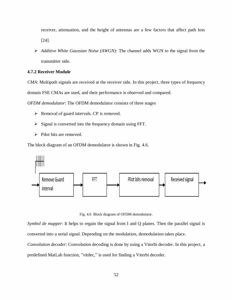
OFDM demodulator: The OFDM demodulator consists of three stages

Removal of guard intervals. CP is removed.

Signal is converted into the frequency domain using FFT.

Pilot bits are removed.

The block diagram of an OFDM demodulator is shown in Fig. 4.6.

Fig. 4.6 Block diagram of OFDM demodulator.

Symbol de mapper: It helps to regain the signal from I and Q planes. Then the parallel signal is

converted into a serial signal. Depending on the modulation, demodulation takes place.

Convolution decoder: Convolution decoding is done by using a Viterbi decoder. In this project, a

predefined MatLab function, ‖vitdec,‖ is used for finding a Viterbi decoder.

53

FEC decoder: Binary data is converted into decimal form and converted into a polynomial. Then

an RS decoder is used.

Resultant data: In the resulting data, the noise is minimized.

4.8 Simulation results

The WiMax OFDM PHY used for comparing the performance of the SDCMA and LSCMA is

shown in Fig. 4.7. Here, the frequency domains of SDCMA and LSCMA are taken, and the

equalizer used is FSE. The guard interval is ¼. The length of the signal is 5000, the step size is

0.0001 for SDCMA, and the stationary channel used is

h(n)=[0.2δ(n)-.09δ(n-1)-.0032δ(n-3); 0.092δ(n-1)-.09δ(n-3);0.8δ(n)-0.1δ(n-2); 0.4δ(n-1)-

0.12δ(n-2)+0.2δ(n-3)].

Fig. 4.7 Comparison of FD-SDCMA adn FD-LSCMA using WiMax OFDM PHY.

4.9 Single Carrier LTE uplink

4.9.1 Introduction

Multiple access schemes play an important role in mobile systems. OFDM used in high speed

data transfer systems like WiMax suffers from envelope fluctuations in the time domain, which

54

leads to a high Peak to Average Power Ratio (PAPR). Because of this, SC-FDM is proposed by

the 3rd Generation Partnership Project (3GPP) using LTE [25]. SC-FDM has low PAPR, which

improves power efficiency. SC-FDM has the same complexity and similar throughput

performance as orthogonal frequency division multiple access [26].

This chapter deals with the comparison of SDCMA and LSCMA using SC-FDM uplink PHY.

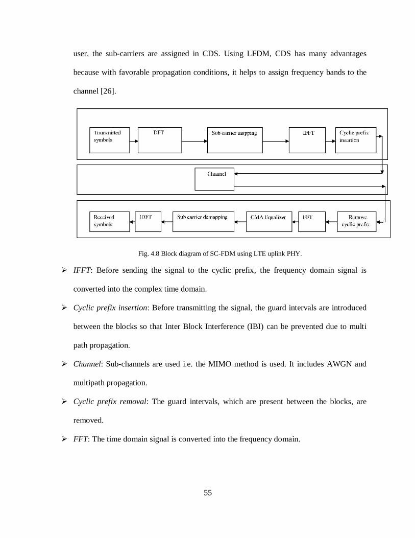
4.10 System model

The block diagram of Single Carrier Frequency Domain Modulation (SC-FDM) using LTE

uplink PHY is shown in Fig. 4.8.

Transmitted symbols: The input data is randomly selected and kept in serial order. Then

these input signals are divided into blocks of equal length. These input blocks are called

transmitted symbols.

DFT: The transmitted symbols are converted into the frequency domain from the time

domain.

Sub-carrier mapping: The frequency domain symbols are mapped to the orthogonal sub-

carriers. The sub-carriers are then divided into two types: Localised FDM (LFDM) and

Distributed FDM (DFDM). In LFDM, sub-carriers are arranged consecutively. In DFDM,

the sub-carriers are distributed equally over the entire bandwidth. The amplitude of the

sub-carrier that is not used is zero. If the ratio of the number of sub-carriers to the number

of transmitted symbols is an integer, then the occupied sub-carriers are equally placed in

the entire bandwidth, and are referred to as Interleaved FDM (IFDM) [25]. The two types

of resource allocation are static sub-carrier mapping and Channel Dependent Scheduling

(CDS). All users using Static Resource Allocation (SRC) are assigned to the same chunk

throughout the communication. According to the channel frequency response of each

55

user, the sub-carriers are assigned in CDS. Using LFDM, CDS has many advantages

because with favorable propagation conditions, it helps to assign frequency bands to the

channel [26].

Fig. 4.8 Block diagram of SC-FDM using LTE uplink PHY.

IFFT: Before sending the signal to the cyclic prefix, the frequency domain signal is

converted into the complex time domain.

Cyclic prefix insertion: Before transmitting the signal, the guard intervals are introduced

between the blocks so that Inter Block Interference (IBI) can be prevented due to multi

path propagation.

Channel: Sub-channels are used i.e. the MIMO method is used. It includes AWGN and

multipath propagation.

Cyclic prefix removal: The guard intervals, which are present between the blocks, are

removed.

FFT: The time domain signal is converted into the frequency domain.

56

CMA Equalization: It helps to perform zero forcing equalization in 3GPP LTE. Here, two

types of CMAs are used, and they are LSCMA and SDCMA. The performances of these

CMAs are observed.

Sub-carrier de-mapping: Here the sub-carriers are removed and the frequency domain

continuous symbols are obtained.

IDFT: Here the frequency domain symbols are converted to the time domain, and these

continuous symbols are the desired symbols at the receiver side.

4.11 Comparison of SDCMA and LSCMA using LTE uplink PHY

Comparison of SDCMA and LSCMA using single carrier frequency division multiplexing and

the LTE uplink is shown in the Fig. 4.9. In this project, the signal length is 5000, the step size is

0.0001 for FD-SDCMA, the number of sub-channels is 4, and the channel used is h(n)=[0.2δ(n)-

.09δ(n-1)-.0032δ(n-3);0.092δ(n-1)-.09δ(n-3);0.8δ(n)-0.1δ(n-2); 0.4δ(n-1)-0.12δ(n-2)+0.2δ(n-3)].

Here, SDCMA and LSCMA are in the frequency domain and the equalizer used is FSE.

4.12 Comparison of SDCMA and LSCMA using WiMax OFDM and LTE uplink PHY

Fig. 4.10 helps us to understand the performance of SDCMA and LSCMA in the frequency

domain using WiMax OFDM PHY, and the LTE uplink using SC-FDM PHY. CMA 22 in the

frequency domain has the best BER performance when compared with the other methods, both

in WiMAX and LTE uplink. When comparing the performance of WiMAX and LTE uplink, the

LTE uplink has better performance, and in this example, FD-CMA 22 in the LTE uplink

performs better when compared with FD-LSCMA and FD-CMA 12.

57

Fig. 4.9 Comparison of FD-SDCMA and FD-LSCMA using LTE uplink PHY.

Fig. 4.10 Comparison of SDCMA and LSCMA using WiMax OFDM PHY and LTE uplink PHY.

58

Chapter 5

CONCLUSION

In this example, CMA 22 performs better in the time domain using a blind equalizer and FSE.

When comparing the performance of the FSE and a blind equalizer, CMA 22 using FSE

performs the best when compared with the other methods. In the frequency domain, SDCMA

and LSCMA using FSE and a blind equalizer obtained optimum BER at the same SNR, but in

this example, CMA 22 using FSE has minimum error compared with the other methods.

Depending on the requirements, any method in the frequency domain can be used to get the best

results. In WiMax and LTE uplink, CMA 22 has minimum BER when compared with the other

techniques, and here, the frequency domain FSE method is used. When compared with WiMax

and SC-FDM, frequency domain FSE CMA22 using the LTE uplink has optimum BER at less

SNR. The minimum error of LSCMA is greater than SDCMA ‘s minimum error and LSCMA‘s

error is unstable . Due to this LSCMA has poor BER performance compared to the SDCMA.

59

References

[1] D. N. Godard, ―Self-recovering equalization and carrier tracking in two-dimensional data

communication systems,‖ IEEE Trans. Commun., vol. 28, no. 11, pp. 1867-1875, Nov.

1980.

[2] J. G. Andrews, A. Ghosh, and R. Muhamed, Fundamentals of WiMAX. Prentice Hall,

Communications Engineering and Emerging Technology Series.

[3] J. Treichler and B. Agee, ―A new approach to multipath correction of constant modulus

signals,‖ in Proc. IEEE Int. Conf. Acoustics, Speech, and Signal Processing, Apr. 1983.

[4] 3GPP Technical Specification 36.211, ver. 8.4.0, ―Physical channels and modulation,‖ Sep.

2008.

[5] 3GPP Technical Specification 36.212, ver. 8.4.0, ―Multiplexing and channel coding,‖ Sep.

2008.

[6] B. Priyanto, H. Codina, S. Rene, T. Sorensen, and P. Mogensen, ―Initial performance

evaluation of DFT-spread OFDM based SC-FDMA for UTRA LTE uplink,‖ in Proc. IEEE

65th Vehicular Technology Conf., VTC-Spring, Apr. 2007, pp. 3175–3179.

[7] B. Agee, ―The least-squares CMA: A new technique for rapid correction of constant

modulus signals,‖ in Proc. IEEE Int. Conf. Acoustics, Speech, and Signal Processing, Apr.

1986

[8] I. Fijalkow, J. Treichler, C. R. Johnson Jr., and C.P. Ensea, ―Fractionally spaced blind

equalizer: Loss of channel disparity,‖ in Proc. IEEE Int. Conf. Acoustics, Speech, and

Signal Processing, 1995.

[9] I. Fijalkow, F. Lopez de Victoria, and C. R. Johnson, Jr., ―Adaptive fractionally spaced

blind equalization,‖ in Proc. IEEE Signal Processing, Oct. 1994, pp. 257-260.

60

[10] J. C. Lee and C. K. Un, ―Performance analysis of frequency-domain block LMS adaptive

filters,‖ IEEE Trans. Circuits Syst., vol. 36, no. 2, pp. 173-189, Feb. 1989.

[11] Y. G. Yang, N. I. Cho, and S. U. Lee, ―Fast blind equalization by using frequency

domain block constant modulus algorithm,‖ in Proc. IEEE Circuits and Systems Conf. (38

Midwest Symposium),1995

[12] ―Mobile WiMax,‖ WiMax Forum.

[13] Wireless MAN group, ―IEEE standard for local and metropolitan area networks.‖

Technical report IEEE Std 802.16-2001, wirelessMAN.org, 2001. Part 16, air interface for

fixed broadband wireless access systems.

[14] T. S. Rappaport, Wireless Communications Principles and Practice, 2nd

edition, 2006.

[15] V. Erceg, K. V. S. Hari, M. S. Smith, D. S. Baum, et al, ―Channel models for fixed

wireless applications,‖ IEEE 802.16.3 Task Group Contributions, Feb. 2001.

[16] S. Yameogo, P. Jacques, and L. Cariou, ―A semi-blind time domain equalization of

SCFDMA signal,‖ in Proc. IEEE. Int. Signal Processing and Information Technology

Conf. (ISSPIT), 2009.

[17] M. M. Rana, M. S. Islam, and A. Z. Kouzani, ―Peak to average power ration analysis for

LTE systems,‖ in Proc. IEEE. Int. Communication Software and Networks Conf., 2010.

[18] Q. Liu, X. Wang, and G. B. Giannakis, ―A cross-layer scheduling algorithm with QoS

support in wireless networks,‖ IEEE Trans. Veh. Technol., vol. 55, no. 3, pp. 839-847, May

2006.