Lal & Barisal, Cogent Engineering (2017), 4: 1318466https://doi.org/10.1080/23311916.2017.1318466

SYSTEMS & CONTROL | RESEARCH ARTICLE

Comparative performances evaluation of FACTS devices on AGC with diverse sources of energy generation and SMESDeepak Kumar Lal1* and A.K. Barisal1

Abstract: This paper deals with automatic generation control of multi area power system using a Fuzzy PID controller. The controller parameters are optimized by Grey Wolf Optimizer (GWO) algorithm. Initially, Hydro-Thermal-Gas two area power systems is considered and superiority of the proposed controller is verified by comparing the results with GWO optimized classical PID controller as well as recently published optimal controller, such as DE-PID and TLBO-PID controllers. The proposed methodology is also verified with a modified power system with a nuclear plant and HVDC link and reveals better performance when compared with sliding mode controller tuned by TLBO algorithm. The proposed controller is designed to stabilize the frequency deviations of nonlinear power system considering FACTS devices and SMES. The results reveal that IPFC seems to be a promising alternative for frequency and tie-line power stabilization. Also the proposed controller is robust and satisfactory towards random step and sinusoidal load patterns.

Subjects: Intelligent Systems; Power Engineering; Systems & Controls

Keywords: automatic generation control; flexible AC transmission system; generation rate constraint; grey wolf optimization algorithm; nuclear power plant

*Corresponding author: Deepak Kumar Lal, Department of Electrical Engineering, Veer Surendra Sai University of Technology Odisha, Burla 768018, IndiaE-mail: laldeepak.sng@gmail.com

Reviewing editor: Wei Meng, Wuhan University of Technology, China

Additional information is available at the end of the article

ABOUT THE AUTHORSDeepak Kumar Lal born in 1984 and received the BTech Degree from the BPUT, Rourkela, Odisha, in 2008 and MTech degree in power system engineering in Electrical Engineering Department, National Institute of Technology, Jamshedpur, India in 2010. Since 2011, he is working as Assistant professor in the Department of Electrical Engineering, Veer Surendra Sai University of Technology, Burla, Odisha, India. His research interests include automatic generation control, economic load dispatch, renewable energy integration and power quality.

A.K. Barisal is an associate professor in the Department of Electrical Engineering, Veer Surendra Sai University of Technology, Burla, Odisha, India since 2006. He received the “Odisha Young Scientist award - 2010”, IEI Young Engineers award - 2010” and “Union Ministry of Power, Department of power prize - 2010” for his outstanding contribution to Engineering and Technology research. His research interests include economic load dispatch, Hydrothermal Scheduling and soft computing applications to power system.

PUBLIC INTEREST STATEMENTAutomatic generation control (AGC) plays an important role to maintain a desired operating point. In an interconnected system, the function of AGC is to exchange and regulate power produced from various power generation units in each area so that the system frequency and the tie-line power interchanges between different control areas are maintained at their scheduled values. With the passage of time new ideas are emerging for the design of AGC controller to improve the system dynamics under the occurrence of the load perturbation. Flexible AC Transmission Systems (FACTS) are capable of enhancing power system stability by controlling the power flow in an interconnected power system. Further, improvement of system dynamics have been revealed with inclusion of storage devices along with FACTS based controller. A comparative study of FACTS devices on AGC have been analyzed in coordination with SMES, which further enhances system dynamics performance to a large extent.

Received: 22 December 2016Accepted: 07 April 2017First Published: 13 April 2017

© 2017 The Author(s). This open access article is distributed under a Creative Commons Attribution (CC-BY) 4.0 license.

Page 1 of 29

Deepak Kumar Lal

Page 2 of 29

Lal & Barisal, Cogent Engineering (2017), 4: 1318466https://doi.org/10.1080/23311916.2017.1318466

1. IntroductionIn a large interconnected power system, the generation of power is normally done by hydro, thermal and nuclear power plants. However, gas power generation is a small percentage of the total power generation which is suitable to meet the varying load demand. In the field of power system opera-tion and control, automatic generation control (AGC) plays an important role in order to maintain a desired operating level characterized by nominal frequency, voltage profile and load flows in power system. In multi area interconnected power system all the generating units are connected together synchronously and work with the same frequency. A small load perturbation in the system will cause the deviations of frequencies of the areas and tie line power deviations from their nominal values (Elgerd, 2008). Therefore, the function of AGC is to exchange and regulate power produced from vari-ous sources in each area so that the system frequency and the tie-line power interchanges between different control areas are maintained at their scheduled values (Bevrani, 2009; Elgerd, 2008; Kothari & Nagrath, 2011). Initially, Elgerd and Fosha have done the pioneering works on AGC for solving regulator design problem (Elgerd & Fosha, 1970a, 1970b). By the passage of time, various controllers such as classical control (Das, Nanda, Kothari, & Kothari, 1990), optimal control (Bhatti, 2014; Elgerd & Fosha, 1970a; Yamashita & Taniguchi, 1986; Yazdizadeh, Ramezani, & Hamedrahmat, 2012), adaptive controls (Oysal, Yilmaz, & Koklukaya, 2005; Pan & Liaw, 1989; Rubaai & Udo, 1994) and robust control (Azzam & Mohamed, 2002; Toulabi, Shiroei, & Ranjbar, 2014; Wang, Zhou, & Wen, 1993) are proposed in AGC study. Though, significant improvements of new controllers in recent years, Proportional Integral Derivative (PID) controller is still an attractive and simple option in AGC. Hence, PID controller is most widely employed in many power industries (Bevrani & Hiyama, 2008; Yu & Tomsovic, 2004). In past decades following the advent of modern intelligent techniques such as Genetic Algorithm (GA), Particle Swarm Optimization (PSO), Fuzzy Logic (FL) and Artificial Neural Network (ANN), new ideas have been emerged for the design of AGC controller to improve the sys-tem dynamics under the occurrence of the load perturbation. The gains of PI and PID controllers are optimized through real coded genetic algorithm in a two area power system (Pingkang, Hengjun, & Yuyun, 2002). A PSO based controller parameter tuning of interconnected reheat thermal system is proposed for AGC in Abdel-Magid and Abido (2003). Artificial Bee Colony (ABC) algorithm has been proposed to tune PI and PID controller’s parameters for interconnected reheat thermal power sys-tem and its superiority is tested by comparing the dynamic performance of the system having PSO tuned controllers (Gozde, Taplamacioglu, & Kocaarslan, 2012). The optimal output feedback control-ler is proposed to the multi-source multi area power system having thermal, hydro and gas power plant in each area (Parmar, Majhi, & Kothari, 2012). Similarly, Teaching Learning Based Optimization (TLBO) algorithm is proposed for the same system for AGC in (Barisal, 2015) and the potential and effectiveness is compared with that of Differential Evolution (DE) and optimal output feedback con-troller proposed in (Mohanty, Panda, & Hota, 2014; Parmar et al., 2012). Few authors proposed hybrid intelligent techniques such as hybrid Bacterial Foraging Optimization Algorithm—PSO (hBFOA-PSO), hybrid Firefly Algorithm—Pattern Search (hFA-PS), hPSO-PS and hDE-PSO for the study of AGC and achieved excellent dynamic performance of the system (Panda, Mohanty, & Hota, 2013; Sahu, Panda, & Padhan, 2015; Sahu, Panda, & Sekhar, 2015; Sahu, Pati, & Panda, 2014). The success of fuzzy logic controllers for AGC of nonlinear power system are reported by many researchers. A self tuning fuzzy PID type controller for AGC of two area interconnected power system is proposed by Yeşil, Güzelkaya, and Eksin (2004). Various heuristic optimization techniques have been incorporated successfully for tuning of fuzzy PID controllers (Sahu, Panda, & Padhan, 2015; Sahu, Panda, & Sekhar, 2015). Similarly, variable structure fuzzy gain scheduling based controller tuned by GA is reported for multi source two area hydro thermal system (Chandrakala, Balamurugan, & Sankaranarayanan, 2013) and output feedback sliding mode controller (SMC) tuned by TLBO algorithm is proposed for multi source two area hydro thermal system with addition of gas plant in one area and nuclear plant in other area (Mohanty, 2015). Distributed optimization and control methods have been applied for economic load dispatch in smart grid (Li, Yu, Yu, Chen, & Wang, 2017; Li, Yu, Yu, Huang, & Liu, 2016). Remodeling of demand side management and development of bidirectional framework for quickly solving problem and getting customers best response is quite encouraging. Due to quite popularity, distributed optimization and control methods are emerging techniques for solving LFC problem. Different level of coordinated communications may be established between the different

Page 3 of 29

Lal & Barisal, Cogent Engineering (2017), 4: 1318466https://doi.org/10.1080/23311916.2017.1318466

controllers. This will lead to establish distributed control mechanism of interconnected realistic power system, which tackles GRC, GDB and load reference set-point constraints.

Further, improvement of system dynamics have been revealed with inclusion of Flexible AC Transmission Systems (FACTS) based controller. These FACTS devices are capable of enhancing power system stability by controlling the power flow in an interconnected power system (Hingorani & Gyugyi, 2000). Several FACTS devices, such as Thyristor Controlled Phase Shifter (TCPS), Static Synchronous Series Compensator (SSSC), Thyristor Controlled Series Compensator (TCSC), Unified Power Flow Controller (UPFC) and Interline Power Flow Controller (IPFC), have been developed and proposed for AGC (Abraham, Das, & Patra, 2007; Chidambaram & Paramasivam, 2012; Lal, Barisal, & Tripathy, 2016; Ngamroo, Taeratanachai, Dechanupaprittha, & Mitani, 2007; Padhan, Sahu, & Panda, 2014; Ponnusamy, Banakara, Dash, & Veerasamy, 2015; Pradhan, Sahu, & Panda, 2016; Shankar, Bhushan, & Chatterjee, 2016; Zare, Hagh, & Morsali, 2015). Energy storage devices have been widely accepted by many researchers for AGC in coordination with FACTS devices. The control performance enhancement of two areas multiple unit power system in coordination with Redox Flow Battery (RFB) and IPFC have been introduced in (Chidambaram & Paramasivam, 2012). Bhatt, Roy, and Ghoshal (2011) compared and described the performance of SMES-SMES, TCPS-SMES and SSSC-SMES controllers in AGC for a two area interconnected power system. The system dynamics in coordina-tion with SSSC and TCPS for two area power system has been studied (Subbaramaiah, 2011).

The literature review reveals that the performance of the power systems not only depend on various controllers but also on the intelligent techniques used for controller parameters optimization. Also the improvements of system dynamics have been achieved with inclusion of FACTS and energy storage devices. In perspective of the above, the ongoing work proposes Fuzzy PID controller for AGC. The controller parameters have been optimized by recently developed powerful optimization technique i.e. Grey Wolf Optimizer (GWO) algorithm (Mirjalili, Mirjalili, & Lewis, 2014). The main advantages of selecting GWO algorithm in the present work is that, the algorithm provides very promising results in various engineering optimization problems. It may be noted that the GWO algorithm requires least number of controlling parameter, which make it simple concept for implementation, effective, faster convergence due to inherent randomness for optimum global solutions. Also, Guha, Roy, and Banerjee (2016) tested the superiority and effectiveness of the GWO algorithm by optimizing the classical controllers such as PI/PID controllers for AGC and compared transient responses of the power system with GA, DE, BFOA, hBFOA-PSO, FA and TLBO optimized classical controllers. Also the comparisons have been done with hPSO-PS and hFA-PS optimized Fuzzy PID controllers.

The motivation behind the present work is that efficient AGC of a complex interconnected power system with FACTS devices coordinated with storage facility greatly improves the dynamic stability of the system when subjected to small load perturbation. In the present work the GWO optimized Fuzzy PID controller is proposed on a two area multi-source interconnected power system and its performance is compared with recently published results such as TLBO-PID, DE-PID and optimal controller for the same power system. Furthermore, proposed controller performance is compared in the modified power system having the output feedback sliding mode controller (SMC) (Mohanty, 2015). Finally, the present work is extended with inclusion of several FACTS devices for AGC and a comparative performance of the system have been analyzed in coordination with SMES. Furthermore, three unequal area thermal power system has been considered to verify the potential of FACTS based controller with the proposed algorithm.

In view of the above discussion, the following are the main objectives of the present work:

(I) Initially, the work is started with AGC of multi-area multi-source hydro-thermal-gas power sys-tem to investigate the superiority of the proposed GWO optimized Fuzzy PID control technique. Then, the work is extended to hydro-thermal-gas in one area and hydro-thermal-nuclear in another area with Super Conducting Magnetic Energy Storage (SMES). Also, to make the system

Page 4 of 29

Lal & Barisal, Cogent Engineering (2017), 4: 1318466https://doi.org/10.1080/23311916.2017.1318466

more realistic nonlinearities like Generation Rate Constraint (GRC) and Governor Dead Band (GDB) is considered for analysis.

(II) To incorporate different types of FACTS devices for AGC of power system and compare their effectiveness to system performance.

(III) To check the stability of different power system models as proposed in this paper, Eigen value analysis has been done.

(IV) To conduct sensitivity analysis for the proposed GWO optimized Fuzzy PID controller for the proposed model and to investigate its robustness to wide changes in loading patterns.

2. Modeling of the interconnected power systemThe system under study is a two area multi source interconnected power system. First the power system model taken into consideration for dynamic behaviour study includes reheat thermal, hydro and gas generating units in each area. Subsequently the study is extended to power system model which includes reheat thermal, hydro and gas generating units in one area. The other area consists of reheat thermal, hydro and nuclear units. The non-linearity such as GRC and GDB is included in the system to make it more realistic power system. The transfer function model of the proposed system is shown in Figure 1 for simulation and AGC study. The system parameters are given in Appendix A.

Figure 1. Transfer function model of multi-source multi-area power system.

UT

UH

UG

Nuclear power plant

Thermal power plant with GRC & Reheat turbine

Thermal power plant with GRC & Reheat turbine

Gas Turbine power plant

Hydro power plant with Governor

U

U

U

UT

UH

UN

Hydro power plant with GovernorDEL F1 (s)

DEL F2 (s)

ACE1

ACE2

Area1

Area2

SSSC/TCPS/UPFC/IPFC

SMES2

SMES1

HVDC

HVDC

f1FACTS

1/R1

1/R31/R2

1

bg.s+cg

Valve Position

1

Tt1.s+1Turbine2

1

Tt1.s+1Turbine1

TR2.s+1

Tgh2.s+1

Transient DroopCompensation2

TR1.s+1

Tgh1.s+1

Transient DroopCompensation1

1

Tdc.s+1

1

Tdc.s+1

1

Tg2.s+1

ThrermalGovernor-2

1

Tg1.s+1

ThrermalGovernor-1

2*pi*T12

s

f2SMES2

SLP2

SLP1

Kr2*Tr2.s+1

Tr2.s+1

Reheat Turbine1

Kr1*Tr1.s+1

Tr1.s+1

Reheat Turbine

GDB

GDB GRC

GRC

GRC

GRCf1SMES1

120

20s+1PS2

120

20s+1PS1

1

Tg2.s+1

NuclearGovernor

1-Kh11-Kr1

Tt1.s +Trh1.s+12LP Turbine1

Kr1

Tt1.s +Trh1.s+12

LP Turbine

KT

KT

KN

KH

KG

KH

-Tw2s+1

0.5*Tw2s+1

Hydro turbine2

-Tw1s+1

0.5*Tw1s+1

Hydro turbine1

1

Trh1.s+1

Hydro Governor1

1

Trh2.s+1

Hydro Governor

Kh1

Tt1.s+1HP Turbine

Xc.s+1

Yc.s+1

Gas Governor

B2

a12

B1

a12

FuzzyPID6

FuzzyPID5

FuzzyPID4

FuzzyPID3

FuzzyPID2

FuzzyPID1

-Tcrs+1

Tf1.s+1

Fuel System1

1

Tcd.s+1Compressor Discharge

System

Add3

1/R11/R3

1/R2

Page 5 of 29

Lal & Barisal, Cogent Engineering (2017), 4: 1318466https://doi.org/10.1080/23311916.2017.1318466

3. Modeling of FACTS devicesFACTS devices are one aspect of the power electronics revolution that is taking place in all areas of electric energy. The principal role is to enhance controllability and power transfer capability in ac system. In this section modeling of the FACTS devices are presented for AGC study.

3.1. Modeling of SSSC for AGCThe SSSC belongs to the family of FACTS devices. It is installed in series with the transmission lines. It has the capability to shift its reactance characteristic from capacitive to inductive and effectively control the power flow. The SSSC is implemented by a voltage sourced converter operated as a syn-chronous voltage source and to provide effective voltage and power flow control in an independent way by internally generated series reactive compensation. It is installed in series with the tie-line for frequency stabilization of interconnected power system. The schematic diagram of SSSC connected in series with the tie-line is shown in Figure 2.

The controller to change the SSSC voltage can be expressed as (Ngamroo et al., 2007; Ponnusamy et al., 2015; Pradhan et al., 2016):

If the frequency deviation ΔF1(s) is sensed, it can be used as the control signal (i.e. ΔError = ΔF1(s)) to the SSSC unit to control Vs which will alter the tie-line power flow between two areas and assist in stabilizing the frequency oscillation. Thus:

(1)ΔVs =

(1 + T

1s

1 + T2s

)(1 + T

3s

1 + T4s

)(K2

1 + TSSSC

s

)

ΔError(s)

(2)ΔPTie(s) =

2�T12

s

[ΔF

1(s) − ΔF

2(s)

]+ K

1

(1 + T

1s

1 + T2s

)(1 + T

3s

1 + T4s

)(K2

1 + TSSSC

s

)

ΔF1

Figure 2. Schematic diagram of SSSC connected in series with the tie-line.

Figure 3. Structure of SSSC as a frequency controller.

Page 6 of 29

Lal & Barisal, Cogent Engineering (2017), 4: 1318466https://doi.org/10.1080/23311916.2017.1318466

where, KSSSC = K1K2

The detailed structure of SSSC in series with tie line is provided in Figure 3. The input signal of SSSC controller is the frequency deviation p.u. Hz in Area 1. The structure of SSSC frequency stabilizers consists of the stabilization gain (KSSSC) block and the phase compensation block with time constants T1, T2, T3 and T4 which provides the appropriate phase-lead characteristics to compensate the lag between input and the output signals.

3.2. Modeling of the TCPS for AGCThe TCPS is a device that changes the relative phase angle between the system voltages. Therefore, the real power flow can be controlled to mitigate the frequency oscillations and improve power system stability (Abraham et al., 2007). A schematic of the two area interconnected power system with TCPS in series with the tie-line is shown in Figure 4. TCPS is placed near Area 1. Resistance of the tie-line is ne-glected. Without TCPS, the incremental tie-line power flow from Area 1 to Area 2 can be expressed as:

where T012

is the synchronizing constant without TCPS and Δf1 and Δf2 are frequency deviations of Area 1 and Area 2 respectively. The detail derivations are presented in Abraham et al. (2007).

The phase shifter angle Δ�(s) with inclusion of TCPS can be represented as:

where Kϕ and TPS are the gain and time constant of the TCPS. Now the tie-line power flow deviation can be written as:

(3)ΔPTie

=2�T

12

s

[ΔF

1(s) − ΔF

2(s)

]+

(1 + T

1s

1 + T2s

)(1 + T

3s

1 + T4s

)(KSSSC

1 + TSSSC

s

)

ΔF1

ΔPTie(s) = ΔP

12(s) + ΔP

SSSC(s)

(5)whereΔPSSSC

(s) =

(1 + T

1s

1 + T2s

)(1 + T

3s

1 + T4s

)(KSSSC

1 + TSSSC

s

)

ΔF1(s)

(6)ΔP0Tie12

=2�T0

12

s

(Δf

1− Δf

2

)

(7)Δ�(s) =K�

1 + sTPSΔError(s)

Figure 4. A schematic diagram of a two area interconnected power system with TCPS in series with tie-line.

Figure 5. Structure of TCPS as frequency stabilizer.

(4)

Page 7 of 29

Lal & Barisal, Cogent Engineering (2017), 4: 1318466https://doi.org/10.1080/23311916.2017.1318466

If the frequency deviation ΔF1(s) is sensed and used as the control signal to the TCPS unit to control

the TCPS phase angle which in turn, control the tie-line power flow, then Equation (7) becomes:

Also the tie-line power flow becomes:

where, ΔPTCPS

(s) = T12

K�

1+sTPSΔF

1(s)

The structure of TCPS as a frequency stabilizer is shown in Figure 5. The gain Kϕ and time constant TPS of the TCPS are optimized using the proposed algorithm.

3.3. Modeling of UPFC for AGCThe Unified Power Flow Controller (UPFC) belongs to an important member in the FACTS family. It has the capability to control, at the same time or specifically every one of the parameters such as voltage, impedance and phase angle which are affecting power flow in the transmission line. In other words, it can independently control both the real and reactive power flow in the line (Hingorani & Gyugyi, 2000). The UPFC consists of two back to back voltage sourced converters as shown in Figure 6. These consecutive converters are worked from a common dc link provided by a dc storage capacitor. Based on the concept on reactive shunt compensation, series compensation and phase angle regulation of power transmission line, the UPFC fulfill all these functions and thereby meet multiple control objectives.

The detail derivations of UPFC based controller for AGC study is given in (Shankar et al., 2016). Thus the UPFC based controller can be represented as follows.

(8)ΔPTie12

(s) =2�T

12

s

[ΔF

1(s) − ΔF

1(s)

]+ T

12

K�

1 + sTPSΔError(s)

(9)Δ�(s) =K�

1 + sTPSΔF

1(s)

(10)ΔPTie12

(s) =2�T

12

s

[ΔF

1(s) − ΔF

2(s)

]+ T

12

K�

1 + sTPSΔF

1(s)

(11)Now ΔPTie12

(s) = ΔP0Tie12

(s) + ΔPTCPS(s)

Figure 6. Schematic diagram of two area interconnected power system with UPFC.

Page 8 of 29

Lal & Barisal, Cogent Engineering (2017), 4: 1318466https://doi.org/10.1080/23311916.2017.1318466

where TUPFC is a time constant of UPFC.

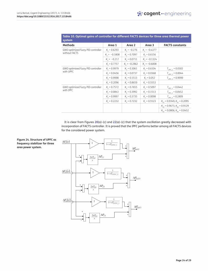
The structure of UPFC as frequency stabilizer is shown in Figure 7.

3.4. Modeling of IPFC for AGCThe IPFC provides a path for the cost-effective utilization of individual transmission lines by encour-aging the autonomous control of both the real and reactive power flow. The IPFC which belongs to FACTS family proposed by Gyugyi with Sen and Schauder in 1998 provides attractive option for com-pensation and power flow management of multiple transmission lines at a given substation (Hingorani & Gyugyi, 2000). The IPFC employs a number of dc-to-ac converters and each provides series compensation for a different line. The schematic of IPFC is shown in Figure 8. It facilitates not only compensation of each transmission line separately but also provides compensation of all at the same time. The IPFC not only provides independent control of reactive series compensation of each individual line, but also provides a capability to directly transfer of real power between the compen-sated lines through dc link. In this way it controls both the real and reactive power transfer through the common dc link from over-loaded lines to under-loaded lines. To understand the impact of IPFC in the power system during the steady state the mathematical derivation is presented in Chidambaram and Paramasivam (2012). The IPFC based controller can be represented in AGC as:

(12)ΔPUPFC

(s) =

{1

1 + sTUPFC

}

ΔF1(s)

(13)ΔPIPFC

(s) =

{1

1 + sTIPFC

}{k1ΔF

1(s) + k

2ΔP

12(s)

}

Figure 7. Structure of UPFC as frequency stabilizer.

Figure 8. Schematic diagram of IPFC.

Page 9 of 29

Lal & Barisal, Cogent Engineering (2017), 4: 1318466https://doi.org/10.1080/23311916.2017.1318466

and

where TIPFC is a time constant of IPFC.

The structure of IPFC as a frequency controller is shown in Figure 9.

4. Modeling of the SMES system for AGCFigure 10 shows the basic transfer function model of SMES unit in power system. An SMES unit has high efficiency and fast response. An SMES unit is designed to store electric power in the low loss superconducting magnetic coil. Its storage capability in addition to kinetic energy of the generator rotor enhances the damping of the electromechanical oscillation in power system. In view of the above, two SMES units are incorporated in Area 1 and Area 2 in order to stabilize frequency oscilla-tions as shown in Figure 1.

The structure for SMES as frequency stabilizer is modeled as the second order lead-lag compensa-tor as shown in Figure 11. The input signals of the SMES units are p.u. frequency deviations in respec-tive areas where those are connected. The parameters of SMES frequency stabilizers in each area such as, the stabilization gain KSMES and time constants T1, T2, T3 and T4 are to be optimized for optimal design of SMES frequency stabilizer.

(14)ΔPTie(s) = ΔP

IPFC(s) + ΔP

12(s)

Figure 9. Structure of IPFC as a frequency controller.

Figure 10. SMES circuit diagram.

Figure 11. Structure of SMES as frequency stabilizer.

Page 10 of 29

Lal & Barisal, Cogent Engineering (2017), 4: 1318466https://doi.org/10.1080/23311916.2017.1318466

5. Controller structure and objective functionThe structure of the Fuzzy PID controller is shown in Figure 12 (Sahu et al., 2014; Yeşil et al., 2004). An identical controller is employed in each area. The error inputs to the controllers are the respective area control error (ACE). For the two areas interconnected power system, the ACE signal made by frequency and tie-line power deviations is represented by Equations (15) and (16),

Fuzzy controller uses error(e) and derivative of error (∙

e) as input signals. The outputs of the Fuzzy controllers UT, UH and UG are the control inputs of the generating units. Fuzzy PID controller is a com-bination of fuzzy proportion-integral (PI) and fuzzy proportional-derivative (PD) controllers. The input scaling factors are K1and K2 and the output scaling factors are K3 and K4. Triangular membership functions are used with five fuzzy linguistic variables such as NB (negative big), NS (negative small), Z (zero), PS (positive small) and PB (positive big) for both the inputs and the output. Membership functions for error, error derivative and FLC output are shown in Figure 13. Mamdani fuzzy inference engine is selected for the present work. The two-dimensional rule base for error, error derivative and FLC output are given in Table 1.

In the selection process of the controller parameters, the objective function is first defined based on the desired specifications and constraints. The output specifications in time domain are peak overshooting, rise time, settling time and steady state errors. In Integral of Time Multiplied Absolute Error (ITAE), time is multiplied with the absolute value of errors so that oscillations die out quickly and results in minimum of settling time (Ogata, 2010). Therefore, it is used as objective function for controller parameters tuning. The objective function J for controller parameters optimization of the interconnected power system is depicted below.

(15)e1(t) = ACE

1= B

1.ΔF

1+ ΔP

Tie

(16)e2(t) = ACE

2= B

2.ΔF

2+ a

12ΔP

Tie

Figure 12. Structure of Fuzzy PID controller.

Figure 13. Membership function for the two inputs and two outputs with gains of −1 to 1 and −10 to 10, respectively.

Page 11 of 29

Lal & Barisal, Cogent Engineering (2017), 4: 1318466https://doi.org/10.1080/23311916.2017.1318466

where, ΔF1 and ΔF2 are the frequency deviations in Area 1 and Area 2 respectively; ΔPTie is the incre-mental change in tie line power; tsim is the time range of simulation. The problem constraints are the minimum and maximum limits of Fuzzy PID controllers scaling factors K1, K2 K3 and K4. Thus, the design problem can be formulated as follows:

Subject to:

6. Grey Wolf Optimizer algorithmThe meta-heuristic optimization techniques have been successfully implemented in many engineer-ing fields. Those have produced excellent results and have many advantages over conventional methods such as simplicity, flexibility, derivative free mechanism and local optima avoidance (Mirjalili et al., 2014). The Grey Wolf Optimizer (GWO) algorithm is one of the meta-heuristic algo-rithms inspired by grey wolves (Canis lupus) (Mirjalili et al., 2014). Grey wolf, also known as timber wolf or western wolf belongs to Canidae family.

The advantage of GWO algorithm over most of the optimization algorithm is that the algorithm requires no specific input parameters. Also, it is straightforward and free from computational com-plexity. The flowchart of GWO algorithm is presented in Figure 14.

The group hunting is an important social behaviour apart from the surviving and living in a pack. The main phases of group hunting are as follows:

(i) Tracking, chasing and approaching the prey.

(ii) Pursuing, encircling and harassing the prey until it stops moving.

(iii) Attack towards the prey.

The mathematical model of social hierarchy of wolves, tracking, encircling and attacking prey are given in Mirjalili et al. (2014).

(17)J = ITAE =

tsim

∫0

(||ΔF1|| + ||ΔF2

|| + ||ΔPTie||). t .dt

(18)Minimize J

(19)Kmin1

≤ K1≤ Kmax

1, Kmin

2≤ K

2≤ Kmax

2, Kmin

3≤ K

3≤ Kmax

3and Kmin

4≤ K

4≤ Kmax

4

Table 1. Fuzzy rules for the inputs and outputsACE ΔACE

NB NS Z PS PBNB NB NB NB NS Z

NS NB NB NS Z PS

Z NB NS Z PS PB

PS NS Z PS PB PB

PB PB Z PS PB PB

Page 12 of 29

Lal & Barisal, Cogent Engineering (2017), 4: 1318466https://doi.org/10.1080/23311916.2017.1318466

Finally, the steps of GWO algorithm may be summarized as follows (Guha et al., 2016):

(a) The search process is started with random initialization of candidate solutions (wolves) in the search space.

(b) Alpha, beta and delta wolves are estimated based on the position of prey.

(c) To find the optimum location of prey, each wolf updates its position.

(d) A control parameter a⃗ linearly decreases from 2 to 0 for better exploitation and exploration of candidate solutions.

(e) Candidate solutions tend to diverge and at the end the optimum solution is stored.

7. Results and discussion of the simulated test system

7.1. Two area test systemThe simulation of system under study has been done in MATLAB/Simulink environment and GWO algorithm has been written in (.m file). The developed model is simulated using initial gain schedul-ing parameters considering an 1% step load perturbation (SLP) in Area 1 at time t = 0 s. The objective function is calculated in .m file and used in optimization algorithm for tuning the gains of Fuzzy PID controller for power system. Series of experiments were conducted to choose the appropriate con-troller parameters. The simulation was repeated for 30 times and the best final solution among the 30 runs is selected as proposed controller parameters. The best final solutions obtained in the 30 runs are considered as optimal solution shown in Table 2 for the system under study.

Figure 14. Flowchart of Grey Wolf Optimizer (GWO) algorithm.

Page 13 of 29

Lal & Barisal, Cogent Engineering (2017), 4: 1318466https://doi.org/10.1080/23311916.2017.1318466

Table 2. GWO optimized Fuzzy PID controller parameters of power system-1 without physical constraintsMethods Area 1 = Area 2GWO optimized controller Thermal Hydro GasFuzzy PID controller K1 = 1.6974 K1 = 0.5428 K1 = 1.5258

K2 = 1.8336 K2 = 0.0605 K2 = 0.1659

K3 = 0.4935 K3 = 1.0157 K3 = 0.3308

K4 = 1.0103 K4 = 1.1712 K4 = 1.0340

Figure 15. (a) Frequency deviation in Area 1 subjected to a step load change of 0.01 p.u. in Area 1, (b) Frequency deviation in Area 2 subjected to a step load change of 0.01 p.u. in Area 1 and (c) Tie-line power flow deviation subjected to a step load change of 0.01 p.u. in Area 1.

0 5 10 15 20 25 30-0.035

-0.03

-0.025

-0.02

-0.015

-0.01

-0.005

0

0.005

Time (s)

∆ F

1 (H

z)

TLBO PID (Barisal, 2015)DE-PID (Mohanty et al., 2014)Optimal Control (Parmar et al., 2012)GWO Fuzzy PIDGWO PID

(a)

0 5 10 15 20 25 30-0.025

-0.02

-0.015

-0.01

-0.005

0

0.005

Time (s)

∆ F

2 (H

z)

TLBO-PID (Barisal, 2015)DE-PID (Mohanty et al., 2014)Optimal Control (Parmar et al., 2012)GWO Fuzzy PID GWO

(b)

0 5 10 15 20 25 30

-6

-4

-2

0

2x 10

-3

Time (s)

∆ P

Tie

(pu

)

TLBO-PID (Barisal, 2015)DE-PID (Mohanty et al., 2014)Optimal Control (Parmar et al., 2012)GWO Fuzzy PID GWO PID

(c)

Page 14 of 29

Lal & Barisal, Cogent Engineering (2017), 4: 1318466https://doi.org/10.1080/23311916.2017.1318466

Figure 16. (a) Frequency deviation in Area 1 subjected to a step load change of 0.01 p.u. in Area 1 and their comparison for proposed GWO optimized Fuzzy PID control scheme with TLBO optimized Output feedback SMC scheme, (b) Frequency deviation in Area 2 subjected to a step load change of 0.01 p.u. in Area 1 and their comparison for proposed GWO optimized Fuzzy PID control scheme with TLBO optimized Output feedback SMC scheme and (c) Tie-line power flow deviation subjected to a step load change of 0.01 p.u. in Area 1 and their comparison for proposed GWO optimized Fuzzy PID control scheme with TLBO optimized Output feedback SMC scheme.

(a)

(b)

(c)

Table 3. GWO optimized Fuzzy PID controllers parameters of power system-2 with HVDC link, GRC and reheat turbineMethods Area 1 = Area 2GWO optimized controller Thermal Hydro GasFuzzy PID controller K1 = 0.2393 K1 = 1.1126 K1 = 1.8334

K2 = 0.5789 K2 = 0.4438 K2 = 1.4036

K3 = 1.8669 K3 = 1.3002 K3 = 0.3902

K4 = 1.4068 K4 = 1.4014 K4 = 1.3604

Page 15 of 29

Lal & Barisal, Cogent Engineering (2017), 4: 1318466https://doi.org/10.1080/23311916.2017.1318466

The predominance of the proposed GWO optimized Fuzzy PID controller is verified in Figure 15(a)–(c), when compared with optimal controller, DE-PID controller, TLBO-PID controller and GWO optimized PID controller for the multi-source two area power system having Hydro-Thermal-Gas in each area considering a 1% SLP in Area 1 at time, t = 0 s. The controller parameters values are given in Table 2. Then, a gas unit in Area 2 is replaced by nuclear unit along with HVDC link, GRC and reheat turbine in each area. The model is simulated with the proposed controller and controller parameters are opti-mized. Results in terms of frequency deviations in each area and tie-line power deviation are shown in Figure 16(a)–(c) by comparing with recently published paper on TLBO optimized output feedback sliding mode controller (SMC). The optimized values for the proposed controllers are presented in Table 3. The performance index values in terms of maximum undershoot (MUS), maximum over-shoot (MOS), settling time with 2% tolerance band and different errors are shown in Table 4. The present work is extended considering GDB with GRC and reheat turbine with inclusion of SMES units in both areas. The comparative analysis of the considered system with proposed controller is done with and without SMES units in each area. It is clear from Figure 17(a)–(c) that system performance further improves with SMES units. Also the Eigen values and minimum damping ratio (MDR) are pre-sented in Table 5. As we know the closed loop system is said to be stable if all the eigen values are located to the left half of the s-plane. From Table 5, it is clear that all eigen values are lying in the left half of s-plane for which the system is stable. The MDR value with SMES and proposed controller is found to be higher than without SMES. The settling time, maximum overshoot (MOS) and minimum undershoot (MUS) are better with SMES as shown in Table 6.

Table 4. Performance evaluation of proposed GWO optimized Fuzzy PID controller by settling time, minimum undershoot and maximum overshootControllers and parameters Proposed GWO fuzzy PID

controllerTLBO optimized output feedback SMC scheme

(Mohanty, 2015)Value Value

Settling times (0.002% band) (s) ΔF1 4.42 20

ΔF2 4.54 9.92

ΔPTie 3.5 20.33

MUS (p.u.) ΔF1 −0.00983358 −0.0123

ΔF2 −0.00175890 −0.0035

ΔPTie −0.00078422 −0.0038

MOS (p.u.) ΔF1 × 10−4 0.0020060735 2.7741

ΔF2 × 10−4 0.00010095 1.2757

ΔPTie × 10−4 0.00005726 8.4175

Performanceindices ITAE 0.0478 0.3684

ITSE 1.9551 × 10−5 9.3287 × 10−4

ISE 3.3554 × 10−5 4.412 × 10−4

IAE 0.0138 0.0611

Page 16 of 29

Lal & Barisal, Cogent Engineering (2017), 4: 1318466https://doi.org/10.1080/23311916.2017.1318466

Further the present work is extended to verify the improvements in system performance with in-corporation of different FACTS devices such as SSSC, TCPS, UPFC and IPFC along with SMES units as shown in Figure 1. The optimal gains of the proposed GWO based Fuzzy PID controller with FACTS devices are reported in Table 7. The comparison of the performance of the system with different FACTS devices are shown in Figure 18(a)–(c). It is clear from Figure 18(a)–(c) that UPFC and IPFC providing good results. If only frequency deviation of Area 1 is considered UPFC performs better than IPFC. But IPFC performs better than UPFC when frequency deviation in Area 2 and tie-line power deviations are also considered. The performance of IPFC is dominating to all FACTS members consid-ered. The performance index values with different FACTS devices are given in Table 8. The overall

Figure 17. (a) Frequency deviation of Area 1 without and with SMES subjected to load change of 0.01 p.u. in Area 1, (b) Frequency deviation of Area 2 without and with SMES subjected to load change of 0.01 p.u. in Area 1 and (c) Tie-line power flow deviation without and with SMES subjected to load change of 0.01 p.u. in Area 1.

(a)

(b)

(c)

Page 17 of 29

Lal & Barisal, Cogent Engineering (2017), 4: 1318466https://doi.org/10.1080/23311916.2017.1318466

Table 5. System modes, minimum damping ratio, for multi-source multi area power system with HVDC link, GDB, GRC and Reheat turbine without and with SMESMethods GWO Fuzzy PID without SMES GWO Fuzzy PID with SMESSystem Modes −2.0000 −2.0000

−0.0348 −2.0000

−5.0000 −0.0348

−2.0000 −3.3333

−0.0348 −3.3333

−3.3333 −0.1000

−3.3333 −12.5000

−0.1000 −5.0000

−12.5000 −0.1000

−0.1000 −12.5000

−12.5000 −0.0348

−5.0000 −5.0000

−19.9809 −36.7400 +23.9350i

−2.2222 + 5.1856i −36.7400 −23.9350i

−2.2222 −5.1856i −36.6879 +23.9109i

−2.4483 +4.9497i −36.6879 −23.9109i

−2.4483 −4.9497i −20.0148

−4.5159 −4.5858

−2.1734 −3.4205 +1.3882i

−1.0459 −3.4205 −1.3882i

−0.4667 −3.3076 +1.3945i

−0.1084 −3.3076 −1.3945i

−0.1435 −0.3401

−5.0000 −0.1098

−2.0000 −0.1431

−2.0000 −1.0409

−2.2554

−1.5745

−1.5505

−5.0000

−2.0000

−2.0000

MDR 0.3939 0.8378

Table 6. Performance evaluation of proposed GWO optimized Fuzzy PID controller by settling time, minimum undershoot and maximum overshoot of multi-source multi area nonlinear power system without and with SMESControllers and parameters Without SMES With SMESSettling times (2% tolerance band) (s) ΔF1 4.42 1.75

ΔF2 4.54 3.68ΔPTie 3.5 2.38

MOS (p.u.) ΔF1 × 10−4 20.0607 1.846ΔF2 × 10−4 1.0095 1.0521ΔPTie × 10−4 0.5726 0.6377

MUS (p.u.) ΔF1 × 10−3 −9.83358 −3.60876ΔF2 × 10−3 −1.75890 −0.88572ΔPTie × 10−3 −0.78422 −0.44698

Page 18 of 29

Lal & Barisal, Cogent Engineering (2017), 4: 1318466https://doi.org/10.1080/23311916.2017.1318466

performance of IPFC is found to be better than others. The eigen values evaluated for the system with coordinated operation of different FACTS devices with an SLP of 1% in Area 1 are presented in Table 9. All eigen values are lying in the left half of s-plane, because of which the system is stable. The MDR value of IPFC based controller is found to be 0.5881, which is higher than others. To approve the adequacy of the proposed approach the analysis is carried out for the system subjected to differ-ent load patterns such as random step load and sinusoidal load. A random step load pattern is pre-sented in Figure 19 and is applied in Area 1. The system responses are given in Figure 20(a)–(c).

Figure 18. (a) Frequency deviation of Area 1 with SMES and FACTS subjected to a step load change of 0.01 p.u. in Area 1, (b) Frequency deviation of Area 2 with SMES and FACTS subjected to a step load change of 0.01 p.u. in Area 1 and (c) Tie-line power flow deviation with SMES and FACTS subjected to a step load change of 0.01 p.u. in Area 1.

(a)

(b)

(c)

Page 19 of 29

Lal & Barisal, Cogent Engineering (2017), 4: 1318466https://doi.org/10.1080/23311916.2017.1318466

Table 7. Optimal gains of controller for different FACTS devicesMethods Area 1 = Area 2 Area 1 = Area 2GWO optimized fuzzy PID controller

Thermal Hydro Gas SMES constants FACTS constants

SSSC K1 = 1.6291 K1 = 0.5978 K1 = 1.8000 T1 = 0.0048 T1 = 0.2933

K2 = 0.3561 K2 = 0.1037 K2 = 0.7356 T2 = 0.0178 T2 = 0.0516

K3 = 1.6633 K3 = 0.7323 K3 = 0.9476 T3 = 0.2393 T3 = 0.5041

K4 = 0.1372 K4 = 0.2603 K4 = 1.6671 T4 = 0.0295 T4 = 0.7684

Ksmes = 0.3649 KSSSC = 0.2830

Tsmes = 0.0405 TSSSC = 0.2254

TCPS K1 = 1.8279 K1 = 1.7430 K1 = 0.2655 T1 = 0.4554 Kϕ = 1.9004

K2 = 0.3036 K2 = 0.4515 K2 = 0.4514 T2 = 0.0509

K3 = 1.8793 K3 = 1.7688 K3 = 1.8824 T3 = 0.4097 TPS = 0.0172

K4 = 1.9604 K4 = 0.5784 K4 = 0.1095 T4 = 0.0265

Ksmes = 0.8695

Tsmes = 0.2268

UPFC K1 = 1.9347 K1 = 1.8720 K1 = 0.2627 T1 = 0.5942 TUPFC = 0.0201

K2 = 0.3568 K2 = 0.3125 K2 = 0.6757 T2 = 0.0587

K3 = 1.2961 K3 = 1.3503 K3 = 1.7661 T3 = 0.4635

K4 = 1.9822 K4 = 0.5819 K4 = 0.3135 T4 = 0.0280

Ksmes = 0.8872

Tsmes = 0.1571

IPFC K1 = 1.9669 K1 = 1.5336 K1 = 0.2389 T1 = 0.5766 KIPFC1 = 0.0270

K2 = 0.3811 K2 = 0.4944 K2 = 0.5364 T2 = 0.0683 KIPFC2 = 0.0016

K3 = 1.5876 K3 = 1.9892 K3 = 1.6987 T3 = 0.4558 TIPFC = 0.0450

K4 = 1.8540 K4 = 0.6728 K4 = 0.3353 T4 = 0.0220

Ksmes = 0.8149

Tsmes = 0.4599

Table 8. Performance criteria for multi-source multi area nonlinear power system with SMES and FACTSObjective function and parameters

SSSC TCPS UPFC IPFC

ITAE 0.0086 0.0072 0.0098 0.0077

ISE 4.5798 × 10−6 7.4202 × 10−7 1.8377 × 10−6 7.7629 × 10−7

ITSE 9.7544 × 10−6 1.4507 × 10−6 2.6448 × 10−6 1.5436 × 10−6

IAE 0.0068 0.0028 0.0043 0.0029

Settling times (2% band) ΔF1 2.34 1.55 1.59000 1.29

ΔF2 3.5 2.01 4.51000 2.25

ΔPTie 2.9 0.66 1.41000 1.41

MUS ΔF1 −0.00503375 −0.00182222 −0.00110808 −0.00217230

ΔF2 −0.00266690 −0.00050430 −0.00175894 −0.00036766

ΔPTie −0.00125826 −0.00026595 −0.00111744 −0.00018922

MOS ΔF1 0.0000014191 0.0002340791 0.0000357620 0.0001321079

ΔF2 0.00000145 0.00005316 0.00021740 0.00005974

ΔPTie 0.00000091 0.00002438 0.00011378 0.00002815

Page 20 of 29

Lal & Barisal, Cogent Engineering (2017), 4: 1318466https://doi.org/10.1080/23311916.2017.1318466

Figure 19. Random load pattern with respect to time.

0 10 20 30 40 50 60 70 80 90 100-2

-1

0

1

2

3

4x 10

-3

Time (s)

∆PL (

p.u)

Figure 20. (a) Frequency deviation in Area 1 subjected to random load in Area 1 with GWO optimized Fuzzy PID controller, (b) Frequency deviation in Area 2 subjected to random load in Area 1 with GWO optimized Fuzzy PID controller and (c) Tie line power deviation obtained subjected to random load in Area 1 with GWO optimized Fuzzy PID controller.

(a)

(b)

(c)

Page 21 of 29

Lal & Barisal, Cogent Engineering (2017), 4: 1318466https://doi.org/10.1080/23311916.2017.1318466

The sinusoidal load perturbation represented by Equation (20) with varying amplitude as shown in Figure 21 is applied in Area 1. The expression for sinusoidal load change is as follows:

Figure 22(a)–(c) show the system response subjected to sinusoidal varying load in Area 1.

(20)ΔPD = 0.03 sin(44.36t) + 0.05 sin(5.3t) − 0.1 sin(6t)

Table 9. System modes, minimum damping ratio, for multi-source multi area nonlinear power system with SMES and FACTSMethods SSSC TCPS UPFC IPFCSystem modes −2.0000

−3.3333 −2.0000 −2.0000 −2.0000

−3.3333 −2.0000 −2.0000 −2.0000

−0.1000 −0.0348 −0.0348 −0.0348

−12.5000 −3.3333 −3.3333 −3.3333

−0.1000 −3.3333 −3.3333 −3.3333

−12.5000 −0.1000 −0.1000 −0.1000

−2.0000 −12.5000 −12.5000 −12.5000

−0.0348 −5.0000 −5.0000 −5.0000

−5.0000 −0.1000 −0.1000 −0.1000

−0.0348 −12.5000 −12.5000 −12.5000

−5.0000 −0.0348 −0.0348 −0.0348

−67.1216 −5.0000 −5.0000 −5.0000

−67.1825 −58.0422 −49.3395 −29.0688 +39.9748i

−22.1978 +21.1799i −28.4684 +56.0027i −27.3788 +77.0634i −29.0688 −39.9748i

−22.1978 −21.1799i −28.4684 −56.0027i −27.3788 −77.0634i −29.1235 +39.9402i

−22.6587 +21.1097i −28.4778 +55.7861i −27.4911 +75.2695i −29.1235 −39.9402i

−22.6587 −21.1097i −28.4778 −55.7861i −27.4911 −75.2695i −22.2410

−19.9981 −20.0000 −20.0001 −20.0018

−19.1607 −2.4292 +1.8917i −5.1713 −4.5571

−3.9637 +4.3612i −2.4292 −1.8917i −5.2122 −3.2550 +1.7917i

−3.9637 −4.3612i −2.5270 +1.8526i −4.4276 −3.2550 −1.7917i

−3.6414 +4.1798i −2.5270 −1.8526i −2.1960 +2.1065i −3.3576 +1.7678i

−3.6414 −4.1798i −0.2774 −2.1960 −2.1065i −3.3576 −1.7678i

−4.4629 +0.0469i −0.1104 −1.9270 +1.6704i −1.0307

−4.4629 −0.0469i −0.1428 −1.9270 −1.6704i −0.2917

−0.3006 −1.0288 −1.0164 −0.1103

−0.1098 −2.1721 −0.1858 −0.1429

−0.1430 −4.3603 −0.1122 −2.1915 +0.0234i

−1.0203 −4.8129 −0.1413 −2.1915 −0.0234i

−1.3976 −4.7465 −2.1659 −2.1701

−2.1496 −5.0000 −5.0000 −5.0000

−5.0000 −2.0000 −2.0000 −2.0000

−2.0000 −2.0000 −2.0000 −2.000

−2.0000

MDR 0.5569 0.4532 0.3348 0.5881

Page 22 of 29

Lal & Barisal, Cogent Engineering (2017), 4: 1318466https://doi.org/10.1080/23311916.2017.1318466

Figure 21. Sinusoidal load pattern with respect to time.

Figure 22. (a) Frequency deviation in Area 1 subjected to sinusoidal load pattern in Area 1 with GWO optimized Fuzzy PID controller with and without FACTS, (b) Frequency deviation in Area 2 subjected to sinusoidal load pattern in Area 1 with GWO optimized Fuzzy PID controller with and without FACTS and (c) Tie line power deviation subjected to sinusoidal load pattern in Area 1 with GWO optimized Fuzzy PID controller with and without FACTS.

(a)

(b)

(c)

Page 23 of 29

Lal & Barisal, Cogent Engineering (2017), 4: 1318466https://doi.org/10.1080/23311916.2017.1318466

Are

a 1

Are

a 2

Are

a 3

P13 P

12

P23

F 1(s)

F2(

s)

F 3(s)

Stea

m T

urbi

ne (r

ehea

t)

Stea

m T

urbi

ne (r

ehea

t)

Gen

erat

ion

Rat

e C

onst

rain

t

Gen

erat

ion

Rat

e C

onst

rain

t

Stea

m T

urbi

ne (r

ehea

t)

SLP

3

SLP

2

SLP

1

1

Tg3.

s+1

Gov

erno

r.

1

Tg2.

s+1

Gov

erno

r

1

Tg1.

s+1

Gov

erno

r

Gen

erat

ion

Rat

e C

onst

rain

t

Fuzz

y PI

DC

ontro

ller3

Fuzz

y PI

DC

ontro

ller2

Fuzz

y PI

DC

ontro

ller1

2*pi

*T23

s ..

2*pi

*T13

s .

Kr3T

r3.s

+1

Tr3.

s+1

'

1

Tt3.

s+1

''a1

3

Kr2T

r2.s

+1

Tr2.

s+1

1 s

a23

Kp3

Tp3.

s+1

a12

Kp2

Tp2.

s+1

du/d

t

1 s

1 s

1/R

3

1/R

2

1

Tt2.

s+1

du/d

t

du/d

t

2*pi

*T12

s

Kp1

Tp1.

s+1

1

Tt1.

s+1

1/R

1

B3

Kr1T

r1.s

+1

Tr1.

s+1

B2B1

Figu

re 2

3. T

rans

fer f

unct

ion

mod

el o

f int

erco

nnec

ted

thre

e ar

ea th

erm

al p

ower

sys

tem

.

Page 24 of 29

Lal & Barisal, Cogent Engineering (2017), 4: 1318466https://doi.org/10.1080/23311916.2017.1318466

It is clear from Figures 20(a)–(c) and 22(a)–(c) that the system oscillation greatly decreased with incorporation of FACTS controller. It is proved that the IPFC performs better among all FACTS devices for the considered power system.

Table 10. Optimal gains of controller for different FACTS devices for three area thermal power systemMethods Area 1 Area 2 Area 3 FACTS constantsGWO optimized fuzzy PID controller without FACTS

K1 = 0.6293 K1 = −0.276 K1 = −0.4377

K2 = −0.1808 K2 = 0.7097 K2 = 0.6156

K3 = −0.217 K3 = 0.0711 K3 = −0.1324

K4 = 0.7757 K4 = −0.2862 K4 = −0.6008

GWO optimized fuzzy PID controller with UPFC

K1 = 0.9979 K1 = 0.3061 K1 = 0.6104 TUPFC_1 = 0.0302

K2 = 0.0456 K2 = 0.0737 K2 = 0.0368 TUPFC_2 = 0.0044

K3 = 0.9998 K3 = 0.1513 K3 = 0.052 TUPFC_3 = 0.9999

K4 = 0.2096 K4 = 0.8659 K4 = 0.5553

GWO optimized fuzzy PID controller with IPFC

K1 = 0.7572 K1 = 0.7655 K1 = 0.5097 TIPFC_1 = 0.0442

K2 = 0.0843 K2 = 0.3992 K2 = 0.1513 TIPFC_2 = 0.0452

K3 = 0.9997 K3 = 0.3735 K3 = 0.0098 TIPFC_3 = 0.2809

K4 = 0.2232 K4 = 0.7232 K4 = 0.5523 Ka1 = 0.9349, Kb1 = 0.2095

Ka2 = 0.9673, Kb2 = 0.9129

Ka3 = 0.0806, Kb3 = 0.0452

Figure 24. Structure of UPFC as frequency stabilizer for three area power system.

Page 25 of 29

Lal & Barisal, Cogent Engineering (2017), 4: 1318466https://doi.org/10.1080/23311916.2017.1318466

7.2. Three unequal area thermal power systemThe system considered is a three unequal area thermal system. Each area of power system consists of speed governor, single stage reheat turbine and generation rate constraint (GRC) of 3%/min. The capacities of different control areas are in the ratio of 2:5:8. The nominal system parameters are presented in Appendix B. The transfer function model of the considered system is shown in Figure 23.

It is concluded from the discussion as presented in Section 7.1 that, overall performance of UPFC and IPFC are superior among others FACTS devices for improvement of power system dynamic per-formance. In order to verify the potential of the UPFC and IPFC based controller, a three area power system is considered in present study. The Structure of UPFC and IPFC as frequency stabilizers for three area power system are shown in Figures 24 and 25, respectively. The system dynamic re-sponses are evaluated and analyzed with 1% SLP in Area 1. The optimal gains of controllers for dif-ferent FACTS devices are given in Table 10. The frequency deviations in Area 1, Area 2 and Area 3 are shown in Figure 26(a)–(c) respectively, subjected to SLP of 1% in Area 1 with GWO optimized Fuzzy PID controller with and without FACTS devices. The IPFC is once again exhibiting greater flex-ibility as far as the dynamics of the system is considered.

Figure 25. Structure of IPFC as frequency stabilizer for three area power system.

Page 26 of 29

Lal & Barisal, Cogent Engineering (2017), 4: 1318466https://doi.org/10.1080/23311916.2017.1318466

8. ConclusionThis paper presents the design and implementation of GWO optimized Fuzzy PID controller in power systems. At first multi-source two area power system having Hydro-Thermal-Gas in each area is considered and the effectiveness and superiority of the proposed GWO optimized Fuzzy PID control-ler for the power system is verified by comparing the results with GWO optimized classical PID con-troller as well as recently published optimal controller, DE-PID and TLBO-PID controllers. Then the considered power system model is modified and a gas unit in Area 2 is replaced by nuclear unit along with HVDC link, GRC and reheat turbine in each area. The comparison is made between GWO optimized Fuzzy PID controller and TLBO optimized output feedback with SMC for the same power

Figure 26. (a) Frequency deviation in Area 1 subjected to SLP of 1% in Area 1 with GWO optimized Fuzzy PID controller with and without FACTS, (b) Frequency deviation in Area 2 subjected to SLP of 1% in Area 1 with GWO optimized Fuzzy PID controller with and without FACTS and (c) Frequency deviation in Area 3 subjected to SLP of 1% in Area 1 with GWO optimized Fuzzy PID controller with and without FACTS.

(a)

(b)

(c)

Page 27 of 29

Lal & Barisal, Cogent Engineering (2017), 4: 1318466https://doi.org/10.1080/23311916.2017.1318466

system. The study reveals that the dynamic performance of the system improves largely with the proposed controller as compared to TLBO optimized output feedback SMC. Then work is extended considering GDB with GRC and reheat turbine with inclusion of SMES units in both areas. The system dynamics is significantly improved in presence of SMES. A comparative study is also presented with coordinated operation of different FACTS controllers for AGC with the proposed controller. Finally sensitivity analysis is carried out to determine the robustness of the system with proposed controller at different load perturbation like random step load and sinusoidal load in Area 1.

FundingThe authors received no direct funding for this research.

Author detailsDeepak Kumar Lal1

E-mail: laldeepak.sng@gmail.comA.K. Barisal1

E-mail: a_barisal@rediffmail.com1 Department of Electrical Engineering, Veer Surendra Sai

University of Technology Odisha, Burla 768018, India.

Citation informationCite this article as: Comparative performances evaluation of FACTS devices on AGC with diverse sources of energy generation and SMES, Deepak Kumar Lal & A.K. Barisal, Cogent Engineering (2017), 4: 1318466.

ReferencesAbdel-Magid, Y.L., & Abido, A.A. (2003). AGC tuning of

interconnected reheat thermal systems with particle swarm optimization. 10th IEEE International Conference on Electronics, Circuits and Systems, Proceedings of the ICECS, 1, 376–379.

Abraham, R. J., Das, D., & Patra, A. (2007). Effect of TCPS on oscillations in tie-power and area frequencies in an interconnected hydrothermal power system. IET Generation, Transmission & Distribution, 1, 632–639. https://doi.org/10.1049/iet-gtd:20060361

Azzam, M., & Mohamed, Y. S. (2002). Robust controller design for automatic generation control based on Q-parameterization. Energy Conversion and Management, 43, 1663–1673. https://doi.org/10.1016/S0196-8904(01)00118-2

Barisal, A. K. (2015). Comparative performance analysis of teaching learning based optimization for automatic load frequency control of multi-source power systems. International Journal of Electrical Power & Energy Systems, 66, 67–77. https://doi.org/10.1016/j.ijepes.2014.10.019

Bevrani, H. (2009). Robust power system frequency control. New York, NY: Springer. https://doi.org/10.1007/978-0-387-84878-5

Bevrani, H., & Hiyama, T. (2008). Robust decentralised PI based LFC design for time delay power systems. Energy Conversion and Management, 49, 193–204. https://doi.org/10.1016/j.enconman.2007.06.021

Bhatt, P., Roy, R., & Ghoshal, S. P. (2011). Comparative performance evaluation of SMES–SMES, TCPS–SMES and SSSC–SMES controllers in automatic generation control for a two-area hydro–hydro system. International Journal of Electrical Power & Energy Systems, 33, 1585–1597. https://doi.org/10.1016/j.ijepes.2010.12.015

Bhatti, T. S. (2014). AGC of two area power system interconnected by AC/DC links with diverse sources in each area. International Journal of Electrical Power & Energy Systems, 55, 297–304.

Chandrakala, K. R. M. V., Balamurugan, S., & Sankaranarayanan, K. (2013). Variable structure fuzzy gain scheduling based load frequency controller for multi source multi area hydro thermal system. International Journal of Electrical Power & Energy Systems, 53, 375–381. https://doi.org/10.1016/j.ijepes.2013.05.009

Chidambaram, I. A., & Paramasivam, B. (2012). Control performance standards based load-frequency controller considering redox flow batteries coordinate with interline power flow controller. Journal of Power Sources, 219, 292–304. https://doi.org/10.1016/j.jpowsour.2012.06.048

Das, D., Nanda, J., Kothari, M. L., & Kothari, D. P. (1990). Automatic generation control of a hydro thermal system with new area control error considering generation rate constraint. Electric Machines & Power Systems, 18, 461–471. https://doi.org/10.1080/07313569008909490

Elgerd, O. I. (2008). Electric energy system theory: An introduction (2nd ed.). McGraw Hill.

Elgerd, O. I., & Fosha, C. E. (1970a). Optimum megawatt-frequency control of multiarea electric energy systems. IEEE Transactions on Power Apparatus and Systems, PAS-89, 556–563. https://doi.org/10.1109/TPAS.1970.292602

Elgerd, O. I., & Fosha, C. E. (1970b). The megawatt-frequency control problem: A new approach via optimal control theory. IEEE Trans Power Apparatus System, PAS-89, 563–577.

Gozde, H., Taplamacioglu, M. C., & Kocaarslan, İ. (2012). Comparative performance analysis of artificial bee colony algorithm in automatic generation control for interconnected reheat thermal power system. International Journal of Electrical Power & Energy Systems, 42, 167–178. https://doi.org/10.1016/j.ijepes.2012.03.039

Guha, D., Roy, P. K., & Banerjee, S. (2016). Load frequency control of interconnected power system using grey wolf optimization. Swarm and Evolutionary Computation, 27, 97–115. https://doi.org/10.1016/j.swevo.2015.10.004

Hingorani, N. G., & Gyugyi, L. (2000). Understanding FACTS: Concepts and technology of FACTS. New York, NY: IEEE Press.

Kothari, D. P., & Nagrath, I. J. (2011). Modern power system analysis. New Delhi: McGraw Hill.

Lal, D. K., Barisal, A. K., & Tripathy, M. (2016). Grey wolf optimizer algorithm based fuzzy PID controller for AGC of multi-area power system with TCPS. Procedia Computer Science, 92, 99–105. https://.doi.org/10.1016/j.procs.2016.07.329

Li, C., Yu, X., Yu, W., Chen, G., & Wang, J. (2017). Efficient computation for sparse load shifting in demand side management. IEEE Transactions on Smart Grid, 8, 250–261. https://doi.org/10.1109/TSG.2016.2521377

Li, C., Yu, X., Yu, W., Huang, T., & Liu, Z. W. (2016). Distributed event-triggered scheme for economic dispatch in smart grids. IEEE Transactions on Industrial Informatics, 12, 1175–1785.

Mirjalili, S., Mirjalili, S. M., & Lewis, A. (2014). Grey wolf optimizer. Advances in Engineering Software, 69, 46–61. https://doi.org/10.1016/j.advengsoft.2013.12.007

Mohanty, B. (2015). TLBO optimized sliding mode controller for multi-area multi-source nonlinear interconnected AGC system. International Journal of Electrical Power & Energy Systems, 73, 872–881. https://doi.org/10.1016/j.ijepes.2015.06.013

Mohanty, B., Panda, S., & Hota, P. K. (2014). Controller parameters tuning of differential evolution algorithm and

Page 28 of 29

Lal & Barisal, Cogent Engineering (2017), 4: 1318466https://doi.org/10.1080/23311916.2017.1318466

its application to load frequency control of multi-source power system. International Journal of Electrical Power & Energy Systems, 54, 77–85. https://doi.org/10.1016/j.ijepes.2013.06.029

Ngamroo, I., Taeratanachai, C., Dechanupaprittha, S., & Mitani, Y. (2007). Enhancement of load frequency stabilization effect of superconducting magnetic energy storage by static synchronous series compensator based on H∞ control. Energy Conversion and Management, 48, 1302–1312. https://doi.org/10.1016/j.enconman.2006.09.017

Ogata, K. (2010). Modern control engineering (5th ed.). New Delhi: Prentice Hall.

Oysal, Y., Yilmaz, A. S., & Koklukaya, E. (2005). A dynamic wavelet network based adaptive load frequency control in power systems. International Journal of Electrical Power & Energy Systems, 27, 21–29. https://doi.org/10.1016/S0142-0615(04)00099-7

Padhan, S., Sahu, R. K., & Panda, S. (2014). Automatic generation control with thyristor controlled series compensator including superconducting magnetic energy storage units. Ain Shams Engineering Journal, 5, 759–774. https://doi.org/10.1016/j.asej.2014.03.011

Pan, C. T., & Liaw, C. M. (1989). An adaptive controller for power system load-frequency control. IEEE Transactions on Power Systems, 4, 122–128. https://doi.org/10.1109/59.32469

Panda, S., Mohanty, B., & Hota, P. K. (2013). Hybrid BFOA–PSO algorithm for automatic generation control of linear and nonlinear interconnected power systems. Applied Soft Computing, 13, 4718–4730. https://doi.org/10.1016/j.asoc.2013.07.021

Parmar, K. P. S., Majhi, S., & Kothari, D. P. (2012). Improvement of dynamic performance of LFC of the two area power system: An analysis using MATLAB. International Journal of Computer Application, 40, 28–32.

Pingkang, L., Hengjun, Z., & Yuyun, L. (2002). Genetic algorithm optimization for AGC of multi-area power systems. TENCON’02 Proceedings, 2002 IEEE Region 10 Conference on Computers, Communications, Control and Power Engineering, 3, 1818–1821.

Ponnusamy, M., Banakara, B., Dash, S. S., & Veerasamy, M. (2015). Design of integral controller for load frequency control of static synchronous series compensator and capacitive energy source based multi area system consisting of diverse sources of generation employing Imperialistic Competition Algorithm. International Journal of Electrical Power & Energy Systems, 73, 863–871. https://doi.org/10.1016/j.ijepes.2015.06.019

Pradhan, P. C., Sahu, R. K., & Panda, S. (2016). Firefly algorithm optimized fuzzy PID controller for AGC of multi-area multi-source power systems with UPFC and SMES. Engineering Science and Technology, an International Journal, 19, 338–354. https://doi.org/10.1016/j.jestch.2015.08.007

Raju, M., Saikia, L. C., & Sinha, N. (2016). Automatic generation control of a multi-area system using ant lion optimizer algorithm based PID plus second order derivative controller. International Journal of Electrical Power & Energy Systems, 80, 52–63. https://doi.org/10.1016/j.ijepes.2016.01.037

Rubaai, A., & Udo, V. (1994). Self-tuning load frequency control: Multilevel adaptive approach. IEE Proceedings Generation,

Transmission and Distribution, 141, 285–290. https://doi.org/10.1049/ip-gtd:19949964

Sahu, B. K., Pati, S., & Panda, S. (2014). Hybrid differential evolution particle swarm optimisation optimised fuzzy proportional–integral derivative controller for automatic generation control of interconnected power system. IET Generation, Transmission & Distribution, 8, 1789–1800. https://doi.org/10.1049/iet-gtd.2014.0097

Sahu, R. K., Panda, S., & Padhan, S. (2015). A hybrid firefly algorithm and pattern search technique for automatic generation control of multi area power systems. International Journal of Electrical Power & Energy Systems, 64, 9–23. https://doi.org/10.1016/j.ijepes.2014.07.013

Sahu, R. K., Panda, S., & Sekhar, G. T. C. (2015). A novel hybrid PSO-PS optimized fuzzy PI controller for AGC in multi area interconnected power systems. International Journal of Electrical Power & Energy Systems, 64, 880–893. https://doi.org/10.1016/j.ijepes.2014.08.021

Shankar, R., Bhushan, R., & Chatterjee, K. (2016). Small-signal stability analysis for two-area interconnected power system with load frequency controller in coordination with FACTS and energy storage device. Ain Shams Engineering Journal, 7, 603–612. https://doi.org/10.1016/j.asej.2015.06.009

Subbaramaiah, K. (2011). Improvement of dynamic performance of SSSC and TCPS based hydrothermal system under deregulated scenario employing PSO based dual mode controller. European Journal of Scientific Research, 57, 230–243.

Toulabi, M. R., Shiroei, M., & Ranjbar, A. M. (2014). Robust analysis and design of power system load frequency control using the Kharitonov’s theorem. International Journal of Electrical Power & Energy Systems, 55, 51–58. https://doi.org/10.1016/j.ijepes.2013.08.014

Wang, Y., Zhou, R., & Wen, C. (1993). Robust load-frequency controller design for power systems. IEE Proceedings C Generation, Transmission and Distribution, 140, 11–16. https://doi.org/10.1049/ip-c.1993.0003

Yamashita, K., & Taniguchi, T. (1986). Optimal observer design for load-frequency control. International Journal of Electrical Power & Energy Systems, 8, 93–100. https://doi.org/10.1016/0142-0615(86)90003-7

Yazdizadeh, A., Ramezani, M. H., & Hamedrahmat, E. (2012). Decentralized load frequency control using a new robust optimal MISO PID controller. International Journal of Electrical Power & Energy Systems, 35, 57–65. https://doi.org/10.1016/j.ijepes.2011.09.007

Yeşil, E., Güzelkaya, M., & Eksin, İ. (2004). Self tuning fuzzy PID type load and frequency controller. Energy Conversion and Management, 45, 377–390. https://doi.org/10.1016/S0196-8904(03)00149-3

Yu, X., & Tomsovic, K. (2004). Application of linear matrix inequalities for load frequency control with communication delays. IEEE Transactions on Power Systems, 19, 1508–1515. https://doi.org/10.1109/TPWRS.2004.831670

Zare, K., Hagh, M. T., & Morsali, J. (2015). Effective oscillation damping of an interconnected multi-source power system with automatic generation control and TCSC. International Journal of Electrical Power & Energy Systems, 65, 220–230. https://doi.org/10.1016/j.ijepes.2014.10.009

Page 29 of 29

Lal & Barisal, Cogent Engineering (2017), 4: 1318466https://doi.org/10.1080/23311916.2017.1318466

© 2017 The Author(s). This open access article is distributed under a Creative Commons Attribution (CC-BY) 4.0 license.You are free to: Share — copy and redistribute the material in any medium or format Adapt — remix, transform, and build upon the material for any purpose, even commercially.The licensor cannot revoke these freedoms as long as you follow the license terms.

Under the following terms:Attribution — You must give appropriate credit, provide a link to the license, and indicate if changes were made. You may do so in any reasonable manner, but not in any way that suggests the licensor endorses you or your use. No additional restrictions You may not apply legal terms or technological measures that legally restrict others from doing anything the license permits.

Appendix

The typical values of system under study are given below:

A.1. Power system-1 (Barisal, 2015; Mohanty et al., 2014; Parmar et al., 2012)

f = 60 Hz; B1 = B2 = 0.425 p.u. MW/Hz; PR = 2,000 MW (rating), PL = 1,740 MW (nominal loading); R1 = R2 = R3 = 2.4 Hz/p.u. MW; pf11 = pf21 = 0.46966; pf12 = pf22 = 0.37814; pf13 = pf23 = 0.1522; Tps = 11.49 s; Kps = 68.9566 Hz/p.u. MW; T12 = 0.0433 p.u.; a12 = −1.

Thermal: Tg1 = Tg2 = 0.08 s; Tr1 = Tr2 = 10 s; Kr1 = Kr2 = 0.3; Tt1 = Tt2 = 0.3 s.

Hydro: Trh1 = Trh2 = 28.75 s; TR1 = TR2 = 5 s; Tgh1 = Tgh2 = 0.2 s; Tw1 = Tw2 = 1 s.

Gas: b1 = b2 = 0.5; c1 = c2 = 1; Xc1 = Xc2 = 0.6 s; Yc1 = Yc2 = 1 s; Tcr1 = Tcr2 = 0.03 s; Tf1 = Tf2 = 0.23 s; Tcd1 = Tcd2 = 0.2 s.

A.2. Power system-2 (Mohanty, 2015)

This is the modified system of power system1 with physical constraints, HVDC link, nuclear power plant in Area 2 are given below:

f = 60 Hz; B1 = B2 = 0.4312 p.u. MW/Hz; PR = 2,000 MW (rating), PL = 1,740 MW (nominal loading); R1 = R2 = R3 = 2.4 Hz/p.u. MW; KT = 0.543478; KH = 0.326084; KN = 0.130438; T12 = 0.545 p.u.; a12 = − 1.

HVDC: Tdc = 0.2 s; Kdc = 1.

Nuclear: KHI = 2; KR1 = 0.3; TT1 = 0.5 s; TRH1 = 7 s; TRH2 = 9 s.

GRC of thermal 3% per minute.

GRC of hydro 360% up and 240% down per minute.

B. Power system-3 (Raju, Saikia, & Sinha, 2016)

f = 60 Hz, Tgi = 0.08 s, Tti = 0.3 s, Tri = 10 s, Kri = 0.5, KPi = 120 Hz/p.u. MW, TPi = 20 s, Hi = 5 s, Di = 8.33 × 10−3 p.u. MW/Hz, Ri = 2.4 Hz/p.u. MW, T12 = 0.0866 p.u. MW/rad, Bi = 0.425 p.u. MW/Hz, Loading = 50%, GRC = 3 min in each area, capacities of different areas are 2:5:8 and SLP = 1 in Area 1.