- 1 -

Comparative Evaluation of Methods to Determine the Earth Pressure Distribution on Cylindrical Shafts: A Review

Tatiana Tobar1 and Mohamed A. Meguid2 1. Tatiana Tobar, Graduate Student

Department of Civil Engineering and Applied Mechanics McGill University, 817 Sherbrooke Street West Montreal, Quebec, Canada H3A 2K6 Email: tatiana.tobarvalencia@mail.mcgill.ca

2. Mohamed A. Meguid*, Assistant Professor Department of Civil Engineering and Applied Mechanics McGill University, 817 Sherbrooke Street West Montreal, Quebec, Canada H3A 2K6 Tel. (514) 398-1537 - Fax. (514) 398-7361 Email: mohamed.meguid@mcgill.ca * Corresponding author

- 2 -

Abstract

Various methods used for calculating and measuring the earth pressure distribution on cylindrical

shafts constructed in sand are evaluated. Emphasis is placed on a comparison between the

calculated earth pressure using different methods for given sand and wall conditions. The effects

of the assumptions made in developing these solutions on the pressure distribution are discussed.

Physical modeling techniques used to simulate the interaction between vertical shafts and the

surrounding soil are presented. The earth pressure measured and the wall movements required to

establish active condition are assessed. Depending on the adopted method of analysis, the

calculated earth pressure distribution on a vertical shaft lining may vary considerably. For

shallow shafts, the theoretical solutions discussed in this study provide consistent estimates of

the active earth pressure. As the shaft depth exceeds its diameter, the solutions become more

sensitive to the ratio between the vertical and horizontal arching and only a range of earth

pressure values can be obtained. No agreement has been reached among researchers as to the

magnitude of wall movement required to establish active conditions around shafts and further

investigations are therefore needed.

Keywords: Cylindrical shafts, earth pressure theory, physical modeling, soil-structure interaction.

- 3 -

1. Introduction

Vertical shafts are widely used as temporary or permanent earth retaining structures for different

engineering applications (e.g. tunnels, pumping stations and hydroelectric projects). Determining

the earth pressure acting on the shaft lining system is essential to a successful design. Classical

earth pressure theories developed by Coulomb (1776) and Rankine (1857) have been often used

to estimate earth pressure on shaft walls. These theories were originally developed for infinitely

long walls under plane strain conditions. Terzaghi (1920) investigated the effect of wall

movement on the magnitude of earth pressure acting on a rigid retaining wall. He concluded that

for dense sand, a wall movement of about 0.1% of the wall height is necessary to reach the

theoretical active earth pressure. Following from the work of Terzaghi (1920), extensive earth

pressure research has been conducted (Terzaghi, 1934, 1954; Rowe, 1969; Bros, 1972; Sherif et

al., 1982, 1984) to determine the wall displacement required for establishing the active stress

state under two-dimensional conditions.

Several theoretical methods have been proposed for the calculation of the active earth pressure

on cylindrical retaining walls supporting granular material (e.g. Berezantzev, 1958; Prater,

1977). However, the earth pressure distribution obtained using these methods was found to vary

significantly. In addition, the required wall movement to reach the calculated pressures is yet to

be understood.

Physical models have been used to measure the changes in earth pressure due to the installation

of model shafts in granular material under normal gravity conditions or in a centrifuge. One of

the key challenges in developing a model shaft is to simulate the radial movement of the

- 4 -

supported soil during construction. Researchers have developed different innovative techniques

to capture these features either during or after the installation of an instrumented lining.

The objective of this study is to review some of the theoretical and experimental techniques to

investigate the active earth pressure on cylindrical shaft linings installed in cohesionless ground.

The assumptions made in developing different theoretical solutions and their effects on the

calculated earth pressure are examined. Finally, a comparison is presented between different

physical modeling techniques used to study the interaction between a shaft lining and the

surrounding soil, and the measured earth pressure distributions are reproduced.

2. Theoretical Methods

When Coulomb (1776) and Rankine (1857) developed their two-dimensional earth pressure

theories, they also established two simple methods of analysis: the limit equilibrium and the slip

line method. Both methods are based on plastic equilibrium, however they differ in how the

solution is obtained. The limit equilibrium method assumes a suitable failure surface, and basic

statics is used to solve for the earth pressure. Conversely, the slip line method assumes the entire

soil mass to be on the verge of failure, and the solution is obtained through a set of differential

equations based on plastic equilibrium. Several attempts have been made to extend these

methods to study the active earth pressure against cylindrical shafts in cohesionless media.

Westergaard (1941) and Terzaghi (1943), proposed analytical solutions; Prater (1977) used the

limit equilibrium method; and Berezantzev (1958), Cheng & Hu (2005), Cheng et al. (2007),

Liu & Wang (2008), Liu et al. (2009) used the slip line method. In contrast to the classical earth

pressure theories, where the active earth pressure calculated using the Coulomb or Rankine

method are essentially the same, the distributions obtained for axisymmetric conditions may

differ considerably depending on the chosen method of analysis, as discussed below.

- 5 -

2.1 Analytical Solutions

The earliest effort to investigate the state of stress around a cylindrical opening in soil was made

by Westergaard (1941), who studied the stress conditions around small unlined drilled holes,

based on the equilibrium of a slipping soil wedge. Terzaghi (1943) extended Westergaard’s

theory to large lined holes, thus proposed a method to calculate the minimum earth pressure

exerted by cohesionless soil on vertical shafts liners. He determined the equilibrium of the

sliding soil mass assuming = v = 1 and r = 3 inside the elastic zone and employing the

Mohr-Coulomb yield criterion. Terzaghi obtained Equations 1 to 3 below for the lateral earth

pressure on a shaft lining. As stated in Equation 3, Terzaghi proposed the use of a reduced angle

of internal friction of the sand, *, to account for the effect of the nonzero shear stresses in the

solution.

11

21)2(

2

1

NnN

nNN

N

N

a

hm (1)

N

N

N n

n

h

a

N

N

nm

n

1

11

1

21 1

1

21*tan

(2)

5* (3)

where, m = p / a, normalized earth pressure; n1 = r / a, normalized extent of the yield zone;

and N = tan2 (45 + */2); a = shaft radius; h = excavation depth; r = radial distance.

Fig. 1a shows the values of normalized earth pressure, m, versus normalized depth, h/a,

originally computed by Terzaghi (1943) for = 40 and those computed by the authors for =

40 and 41. For = 40 the difference between the calculated and original data is rather small.

Increasing the friction angle from 40 to 41 causes a reduction in the normalized earth pressure

- 6 -

by approximately 9%. These numerical values were obtained using the reduced friction angle

given by Eq. 3. The values of m are computed from Eq. 2 for different assumed values of n1

and the corresponding values of h/a are then computed from Eq. 1. The procedure is detailed by

Terzaghi (1943).

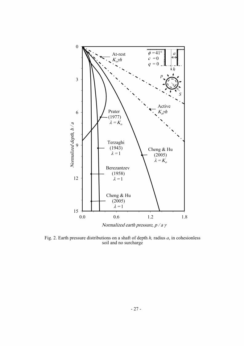
Fig. 2 shows, among other solutions, the calculated earth pressure distribution with depth using

the above equations for a shaft lining of radius, a, and height, h, installed in cohesionless soil

with = 41o. The pressure generally increases with depth and reaches a normalized value, p/a,

of 0.25 at a depth of approximately 5 times the shaft radius. For h/a greater that 5, the pressure

increase is less significant and reaches a normalized value, p/a, of 0.30 at a depth of

approximately 15 times the shaft radius.

2.2 Limit equilibrium

Prater (1977) adapted Coulomb wedge theory for axisymmetric conditions assuming a conical

failure surface. He introduced into the analysis tangential and radial forces, T and F (See Fig.

1c). The force T is a function of the earth pressure coefficient on radial planes, λ, which is

defined by the stress ratio σθ / σv. Prater argued that λ is a decisive parameter whose value should

range between Ka and Ko and not equal to unity as was implicitly assumed by Terzaghi (1943).

The earth pressure (force per unit length of the shaft circumference) P1 is expressed by Eq. 4,

where Kr is the coefficient of earth pressure for cylindrical shafts given by Eq. 5.

21 5.0 hKP r

(4)

3tan3

1tan

tan

h

a

a

hK r

(5)

- 7 -

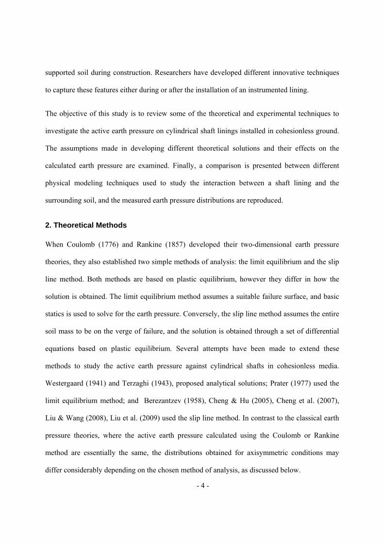
where, a = shaft radius; h = excavation depth; = inclination of failure surface; = angle

between the reaction Q acting on the sliding body and the normal ( = - for active condition); λ

= coefficient of lateral earth pressure on radial planes.

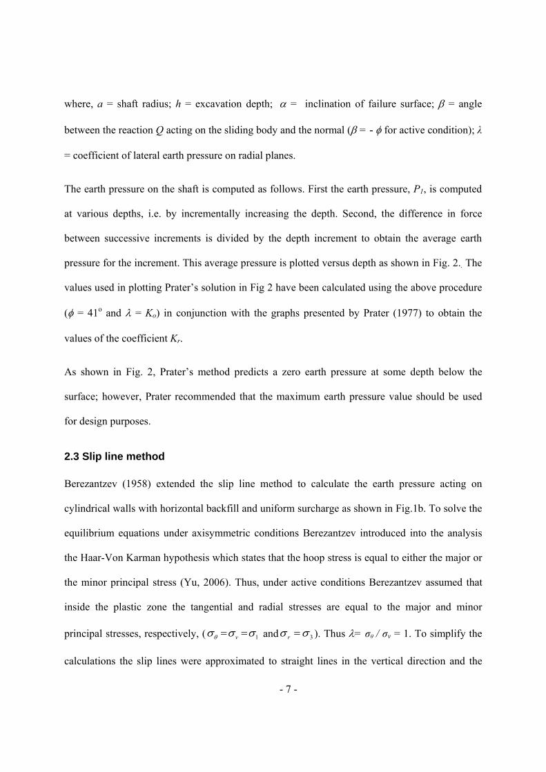
The earth pressure on the shaft is computed as follows. First the earth pressure, P1, is computed

at various depths, i.e. by incrementally increasing the depth. Second, the difference in force

between successive increments is divided by the depth increment to obtain the average earth

pressure for the increment. This average pressure is plotted versus depth as shown in Fig. 2.. The

values used in plotting Prater’s solution in Fig 2 have been calculated using the above procedure

( = 41o and = Ko) in conjunction with the graphs presented by Prater (1977) to obtain the

values of the coefficient Kr.

As shown in Fig. 2, Prater’s method predicts a zero earth pressure at some depth below the

surface; however, Prater recommended that the maximum earth pressure value should be used

for design purposes.

2.3 Slip line method

Berezantzev (1958) extended the slip line method to calculate the earth pressure acting on

cylindrical walls with horizontal backfill and uniform surcharge as shown in Fig.1b. To solve the

equilibrium equations under axisymmetric conditions Berezantzev introduced into the analysis

the Haar-Von Karman hypothesis which states that the hoop stress is equal to either the major or

the minor principal stress (Yu, 2006). Thus, under active conditions Berezantzev assumed that

inside the plastic zone the tangential and radial stresses are equal to the major and minor

principal stresses, respectively, ( 1 v and 3 r ). Thus = σθ / σv = 1. To simplify the

calculations the slip lines were approximated to straight lines in the vertical direction and the

- 8 -

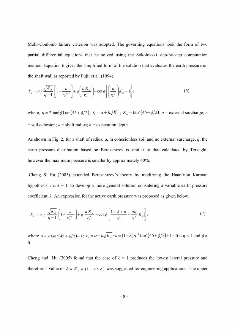
Mohr-Coulomb failure criterion was adopted. The governing equations took the form of two

partial differential equations that he solved using the Sokolovski step-by-step computation

method. Equation 6 gives the simplified form of the solution that evaluates the earth pressure on

the shaft wall as reported by Fujii et al. (1994).

cKr

a

r

Kaq

r

aKaP a

bb

a

b

aa

1cot1

1 1

(6)

where, 245tantan2 ; ab Khar ; 245tan2 aK ; q = external surcharge; c

= soil cohesion; a = shaft radius; h = excavation depth

As shown in Fig. 2, for a shaft of radius, a, in cohesionless soil and no external surcharge, q, the

earth pressure distribution based on Berezantzev is similar to that calculated by Terzaghi,

however the maximum pressure is smaller by approximately 40%.

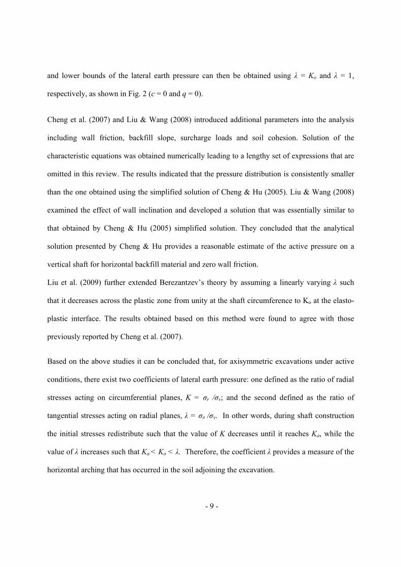
Cheng & Hu (2005) extended Berezantzev’s theory by modifying the Haar-Von Karman

hypothesis, i.e. λ = 1, to develop a more general solution considering a variable earth pressure

coefficient, λ. An expression for the active earth pressure was proposed as given below.

cKr

a

r

Kaq

r

aKaP a

bb

a

b

aa

1cot1

1 1

(7)

where 1245tan 2 ; ab Khar ; 1245tan)1( 21 ; 0 < η < 1 and

0.

Cheng and Hu (2005) found that the case of λ = 1 produces the lowest lateral pressure and

therefore a value of )sin1( oK was suggested for engineering applications. The upper

- 9 -

and lower bounds of the lateral earth pressure can then be obtained using λ = Ko and λ = 1,

respectively, as shown in Fig. 2 (c = 0 and q = 0).

Cheng et al. (2007) and Liu & Wang (2008) introduced additional parameters into the analysis

including wall friction, backfill slope, surcharge loads and soil cohesion. Solution of the

characteristic equations was obtained numerically leading to a lengthy set of expressions that are

omitted in this review. The results indicated that the pressure distribution is consistently smaller

than the one obtained using the simplified solution of Cheng & Hu (2005). Liu & Wang (2008)

examined the effect of wall inclination and developed a solution that was essentially similar to

that obtained by Cheng & Hu (2005) simplified solution. They concluded that the analytical

solution presented by Cheng & Hu provides a reasonable estimate of the active pressure on a

vertical shaft for horizontal backfill material and zero wall friction.

Liu et al. (2009) further extended Berezantzev’s theory by assuming a linearly varying λ such

that it decreases across the plastic zone from unity at the shaft circumference to Ko at the elasto-

plastic interface. The results obtained based on this method were found to agree with those

previously reported by Cheng et al. (2007).

Based on the above studies it can be concluded that, for axisymmetric excavations under active

conditions, there exist two coefficients of lateral earth pressure: one defined as the ratio of radial

stresses acting on circumferential planes, K = σr /σv; and the second defined as the ratio of

tangential stresses acting on radial planes, λ = σθ /σv. In other words, during shaft construction

the initial stresses redistribute such that the value of K decreases until it reaches Ka, while the

value of λ increases such that Ka < Ko < λ. Therefore, the coefficient λ provides a measure of the

horizontal arching that has occurred in the soil adjoining the excavation.

- 10 -

2.4 Comparison between different theoretical solutions

A summary of the earth pressure distribution calculated using some of the above methods for a

given shaft geometry (height, h and radius, a) and soil property () is presented in Fig. 2.

Although all methods predict pressures that are less than the at-rest and active values, the

distributions of earth pressure with depth notably differ. The Terzaghi and Berezantzev methods

implicitly assume λ equals unity, leading to a minimum value of the active earth pressure. This is

consistent with the results of the plastic equilibrium and slip line methods. Both solutions result

in pressure distributions that ultimately reach a constant earth pressure at some depth below

surface. As discussed earlier, Prater’s method predicts a different pressure distribution that can

be characterized (for the same shaft geometry and soil conditions) by a rapid increase in pressure

up to a depth of about 4.5 times the shaft radius and then a decrease to zero at a depth of 8.5

times the shaft radius. The solution of Cheng & Hu provided the lower and upper bounds of the

lateral earth pressure as given by λ = 1 and λ = Ko, respectively. For λ = 1 the earth pressure is

the same as that calculated using the Berezantzev method. Fig. 2 shows that for shallow shafts,

where the shaft height ranges from 1 to 2 times the shaft radius, the difference between the above

theoretical methods is insignificant.

3. Experimental Investigations

Several studies have been conducted to measure the earth pressure distribution due to the

installation of a model shaft in granular material. To simulate the lining installation and the radial

soil movement during construction, different techniques have been developed that can be

grouped into three main categories: (a) shaft sinking; (b) temporary stabilization of the

excavation using fluid pressure (liquid or gas); and (c) the use of a mechanically adjustable

- 11 -

lining. These techniques are briefly described and samples of the experimental results are

presented.

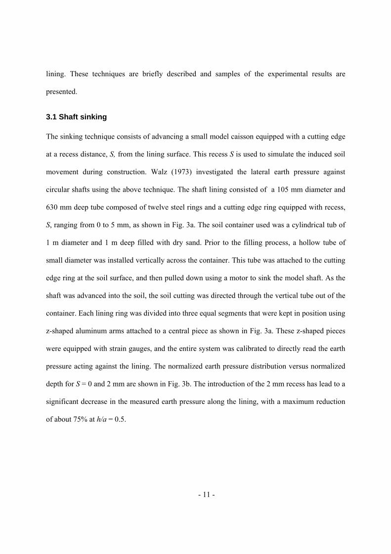
3.1 Shaft sinking

The sinking technique consists of advancing a small model caisson equipped with a cutting edge

at a recess distance, S, from the lining surface. This recess S is used to simulate the induced soil

movement during construction. Walz (1973) investigated the lateral earth pressure against

circular shafts using the above technique. The shaft lining consisted of a 105 mm diameter and

630 mm deep tube composed of twelve steel rings and a cutting edge ring equipped with recess,

S, ranging from 0 to 5 mm, as shown in Fig. 3a. The soil container used was a cylindrical tub of

1 m diameter and 1 m deep filled with dry sand. Prior to the filling process, a hollow tube of

small diameter was installed vertically across the container. This tube was attached to the cutting

edge ring at the soil surface, and then pulled down using a motor to sink the model shaft. As the

shaft was advanced into the soil, the soil cutting was directed through the vertical tube out of the

container. Each lining ring was divided into three equal segments that were kept in position using

z-shaped aluminum arms attached to a central piece as shown in Fig. 3a. These z-shaped pieces

were equipped with strain gauges, and the entire system was calibrated to directly read the earth

pressure acting against the lining. The normalized earth pressure distribution versus normalized

depth for S = 0 and 2 mm are shown in Fig. 3b. The introduction of the 2 mm recess has lead to a

significant decrease in the measured earth pressure along the lining, with a maximum reduction

of about 75% at h/a = 0.5.

- 12 -

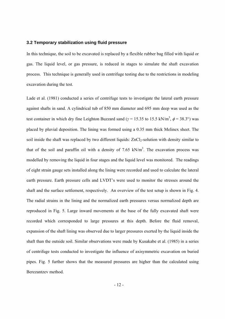
3.2 Temporary stabilization using fluid pressure

In this technique, the soil to be excavated is replaced by a flexible rubber bag filled with liquid or

gas. The liquid level, or gas pressure, is reduced in stages to simulate the shaft excavation

process. This technique is generally used in centrifuge testing due to the restrictions in modeling

excavation during the test.

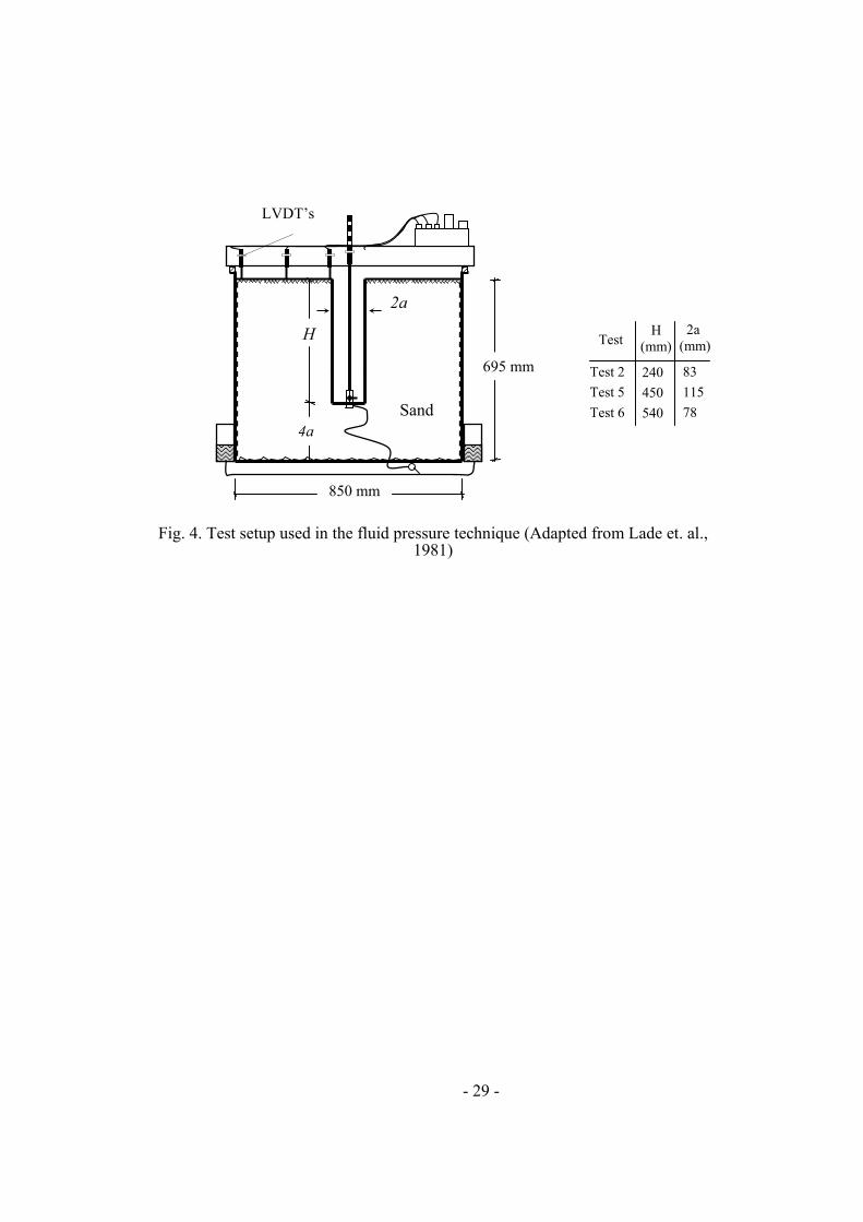
Lade et al. (1981) conducted a series of centrifuge tests to investigate the lateral earth pressure

against shafts in sand. A cylindrical tub of 850 mm diameter and 695 mm deep was used as the

test container in which dry fine Leighton Buzzard sand (γ = 15.35 to 15.5 kN/m3, = 38.3) was

placed by pluvial deposition. The lining was formed using a 0.35 mm thick Melinex sheet. The

soil inside the shaft was replaced by two different liquids: ZnCl2-solution with density similar to

that of the soil and paraffin oil with a density of 7.65 kN/m3. The excavation process was

modelled by removing the liquid in four stages and the liquid level was monitored. The readings

of eight strain gauge sets installed along the lining were recorded and used to calculate the lateral

earth pressure. Earth pressure cells and LVDT’s were used to monitor the stresses around the

shaft and the surface settlement, respectively. An overview of the test setup is shown in Fig. 4.

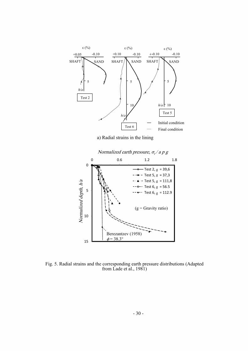
The radial strains in the lining and the normalized earth pressures versus normalized depth are

reproduced in Fig. 5. Large inward movements at the base of the fully excavated shaft were

recorded which corresponded to large pressures at this depth. Before the fluid removal,

expansion of the shaft lining was observed due to larger pressures exerted by the liquid inside the

shaft than the outside soil. Similar observations were made by Kusakabe et al. (1985) in a series

of centrifuge tests conducted to investigate the influence of axisymmetric excavation on buried

pipes. Fig. 5 further shows that the measured pressures are higher than the calculated using

Berezantzev method.

- 13 -

Konig et al. (1991) carried out a series of centrifuge tests to study the effects of the shaft face

advance on a pre-installed lining. The model shaft consisted of two sections: an upper section

made of rigid tube to simulate the installed lining, and a lower section made of rubber membrane

to model the unsupported area of the excavation. At the initial condition, the membrane was

pressurized with air to equilibrate the pressure exerted by the soil. To simulate the shaft face

advance, the air pressure was incrementally reduced. The lateral movement of the rubber

membrane was monitored using LVDT’s embedded in the sand; the stresses in the shaft lining

were monitored using strain gauges installed at different distances from the end of the lining.

Results indicated that for dry sand, only a small support pressure was needed to maintain

stability. However, there was a significant load transfer to the lining closest to the excavation

face due to arching and stress redistribution in the soil.

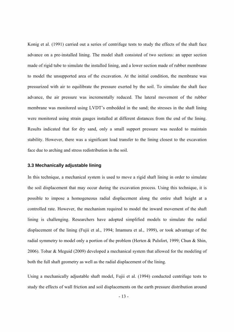
3.3 Mechanically adjustable lining

In this technique, a mechanical system is used to move a rigid shaft lining in order to simulate

the soil displacement that may occur during the excavation process. Using this technique, it is

possible to impose a homogeneous radial displacement along the entire shaft height at a

controlled rate. However, the mechanism required to model the inward movement of the shaft

lining is challenging. Researchers have adopted simplified models to simulate the radial

displacement of the lining (Fujii et al., 1994; Imamura et al., 1999), or took advantage of the

radial symmetry to model only a portion of the problem (Herten & Pulsfort, 1999; Chun & Shin,

2006). Tobar & Meguid (2009) developed a mechanical system that allowed for the modeling of

both the full shaft geometry as well as the radial displacement of the lining.

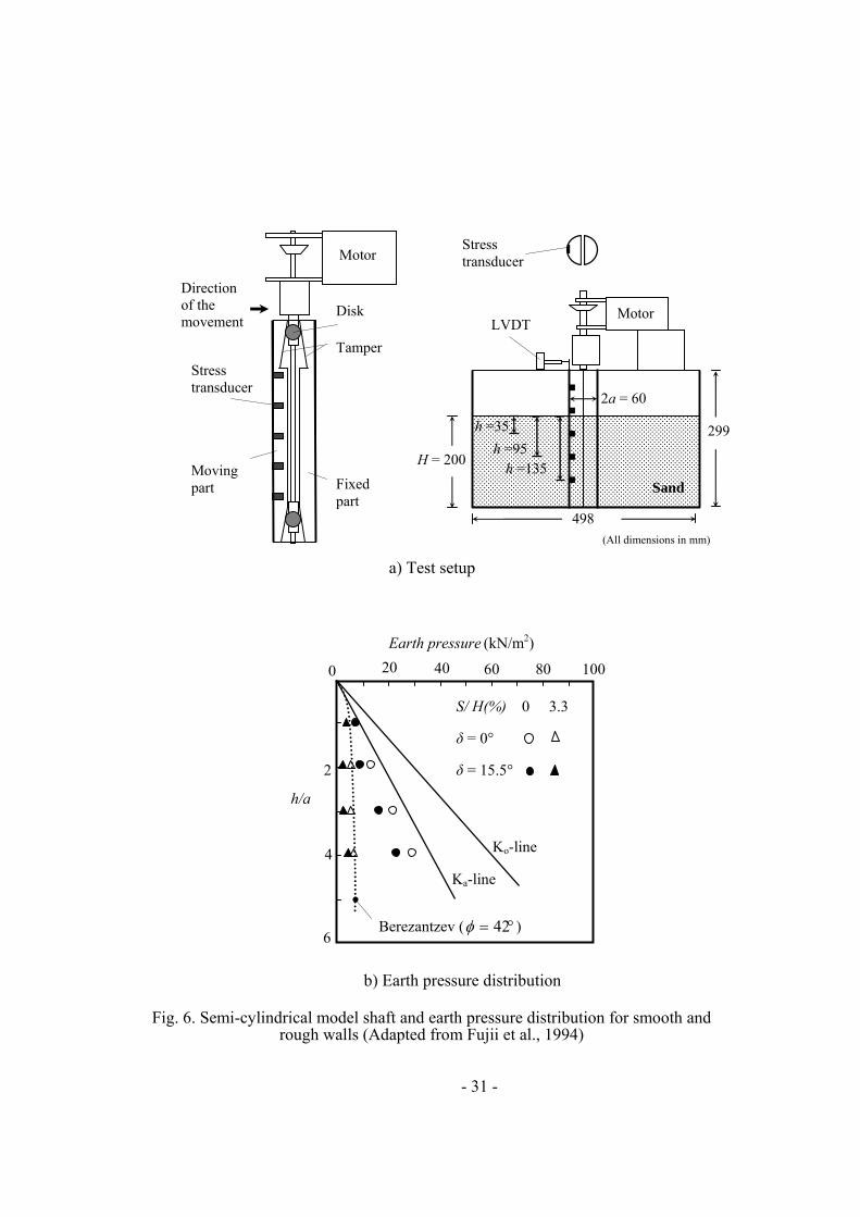
Using a mechanically adjustable shaft model, Fujii et al. (1994) conducted centrifuge tests to

study the effects of wall friction and soil displacements on the earth pressure distribution around

- 14 -

rigid shafts. The lining was made of an aluminum cylinder of 60 mm in diameter split vertically

into two semi-cylinders; one-half was instrumented with small stress transducers and

horizontally moved using a motor to simulate the radial displacement of the shaft lining. Details

of the apparatus are shown in Fig. 6a. The model shaft was placed into a rectangular soil

container and Toyoura dry sand was rained around it up to 200 mm in height, H. Four tests were

conducted for different densities and wall friction conditions. The measured earth pressure

versus normalized depth for dense sand ( = 42, γ = 14.7 kN/m3) and different wall friction is

shown in Fig. 6b along with the earth pressure calculated from Berezantzev method. The

experimental results show good agreement with the theoretical solution of Berezantzev (1958).

Little change in the measured earth pressure was reported at displacements greater than 1% of

the wall height, H (6.6% of the shaft radius), and the wall friction was found to have a negligible

effect on the measured earth pressure distribution.

Imamura et al. (1999) developed a model shaft similar to that used by Fujii et al. (1994).

However, the instrumented semi-cylinder was horizontally translated using an external

mechanism attached to a motor. Air-dried Toyoura sand with = 42 and γ = 15.2 kN/m3 was

used during the four centrifuge tests conducted to study the development of the active earth

pressure around shafts and the extent of the yield zone. They concluded that the earth pressure

decreases with increasing wall displacement until it coincides with Berezantzev’s solution at a

wall displacement that corresponds to 0.2% of the wall height, H (1.6% of the shaft radius). The

maximum extent of the yield zone was found to be approximately 0.7 times the shaft diameter.

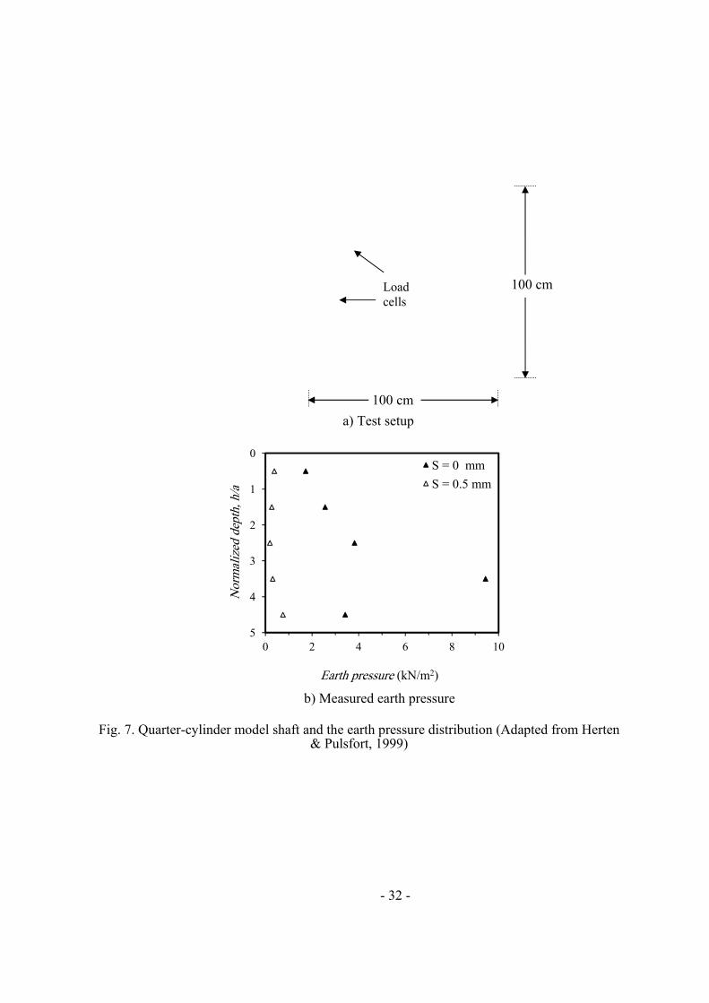
Herten & Pulsfort (1999) took advantage of the radial symmetry of the problem and modeled

only one quadrant of the shaft. The test setup consisted of one quarter of a cylindrical shaft with

0.4 m in diameter and 1 m long. The model shaft was placed along one corner of a rectangular

- 15 -

box of 1 x 1 m in plan and 1.2 m in height. To minimize the wall friction, the walls were

lubricated using Teflon film and oil. The test container was filled using pluvial deposition with

dry fine sand of = 41 in dense state (36% porosity). The shaft lining was horizontally moved

using a motor to simulate the radial displacement of the shaft. Details of the test setup and the

results of one of the four tests conducted are shown in Fig. 7. Little change in the measured

lateral earth pressure occurred for wall displacements greater than 0.05% of the wall

height(0.25% of the shaft radius).

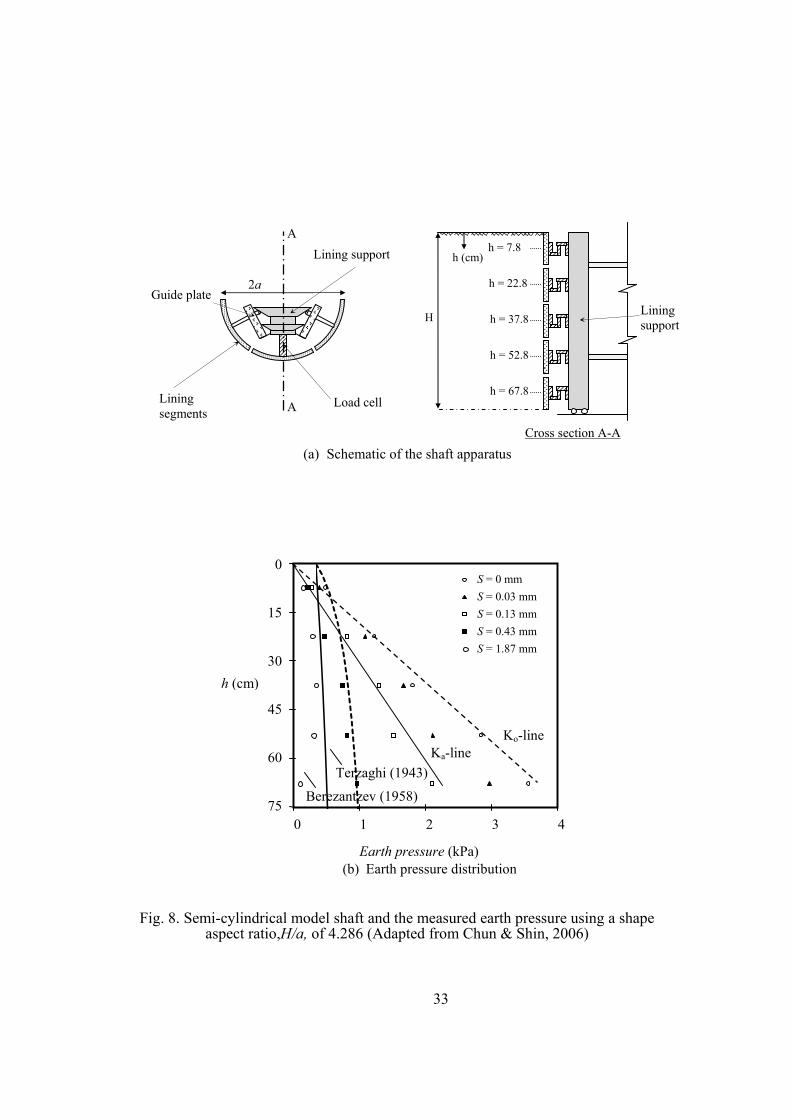
Chun & Shin (2006) conducted model tests to study the effects of wall displacement and shaft

size on the earth pressure distribution using a mechanically adjustable semi-circular shaft. The

lining was made from an acrylic semi-cylinder that was cut longitudinally into three equal

segments, i.e. each span an angle of 60°, to accommodate the changes in diameter during testing.

Transversally the shaft was divided into five equal segments; some of them were used as

sensitive areas for load cells installed behind the lining. Fig. 8a shows a schematic of the model.

The soil container used was a rectangular box, 0.7 m wide, 1 m long and 0.75 m deep filled with

dry sand ( = 41.6; γ = 16.4 kN/m3; Dr = 81%). Three different shaft radii, a, equal to 0.175,

0.15 and 0.115 m, and a constant depth, H = 0.75 m, were tested. The reported earth pressure

versus depth at various wall displacements for a smooth shaft and aspect ratio, H/a, equal to

4.286 are presented in Fig. 8b. The results indicate that earth pressure decreased with increasing

wall movement and became minimum when the wall movement reached 0.6 to 1.8% of the wall

height. In Fig. 8 the earth pressure calculated from Berezantzev and Terzaghi methods are shown

for comparison. It appears from this comparison that the measured earth pressures are higher

than that predicted from Berezantzev; Terzaghi`s distribution falls between the measured earth

pressure at S equal to 0.43 and 1.87 mm (0.06% and 0.25% of the wall height, H). Chun & Shin

- 16 -

(2006) found that soil failure extended a distance of approximately one shaft radius from the

outer perimeter of the lining.

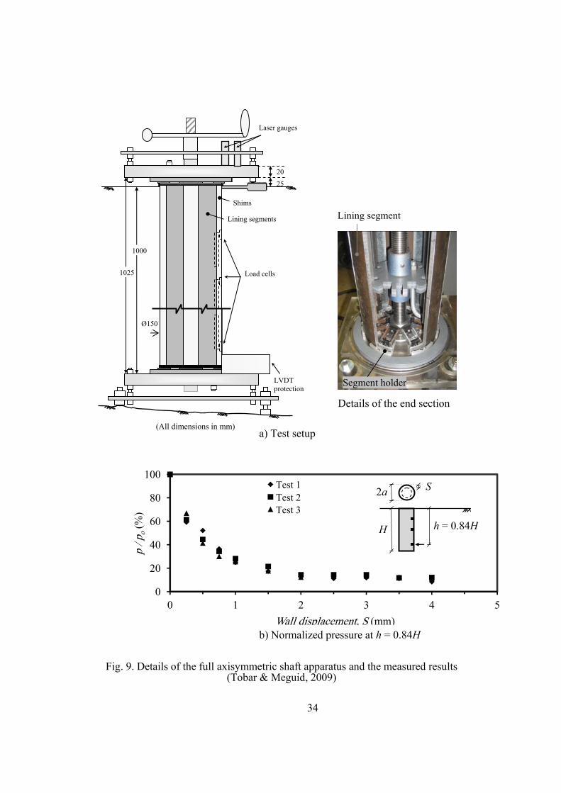
Tobar & Meguid (2009) conducted a series of tests under normal gravity to investigate the

changes in lateral earth pressure due to radial displacement of the shaft lining. The developed

apparatus allowed for the modeling of both the full geometry of the shaft and the radial

displacement of the lining. It was built using six curved lining segments held vertically using

segment holders (Fig. 9a). A simple mechanism was developed to translate the lining segments

radially; it consisted mainly of steel hinges that connected the segment holders to central nuts.

These nuts pass through a central threaded rod extended along the shaft axis. As the axial rod

was rotated, the nuts moved vertically, pulling the segment holders radially inwards and

consequently the shaft lining was uniformly translated.

The model shaft (0.15 m in diameter and 1 m long) was placed into a circular container of 1.22

m diameter and 1.07 m depth. The container was filled with coarse dry sand ( = 41; γ = 14.7

kN/m3) using pluvial deposition. The axisymmetric active earth pressure fully developed when

the wall displacements, S, ranged between 0.2% and 0.3% of the wall height, H. It was

concluded that for S 0.1% H, the measured pressures fell into the range predicted by Cheng &

Hu (2005); and that at S 0.3 % H, the measured pressures closely followed the pressure

distributions calculated using Terzaghi (1943) and Berezantzev (1958) methods.

3.4 Discussion of experimental investigations

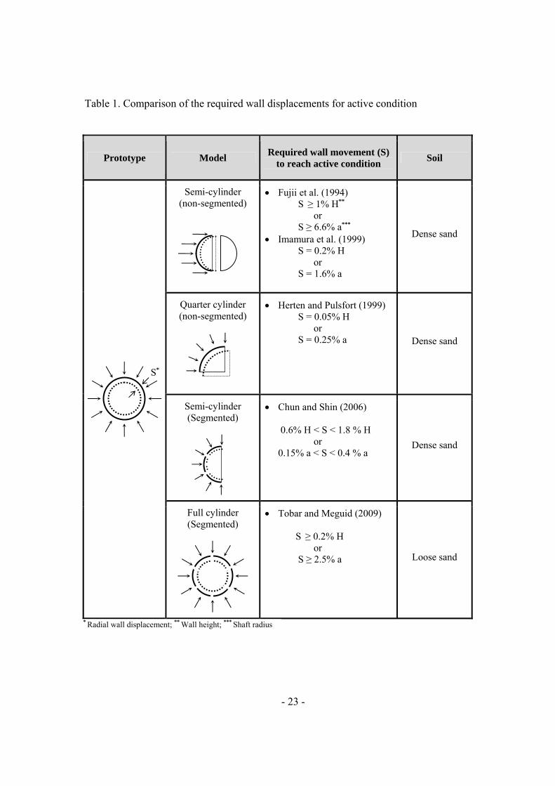
Table 1 shows a summary of the required wall displacement for establishing active conditions.

To simplify the design and operation of the shaft models, simplified mechanisms were used to

reduce the shaft diameter uniformly. It is evident that no agreement has been reached among

- 17 -

researchers as to the required wall movement to reach active conditions. The displacement

ranged from 0.05% to 1.8% of the shaft height as shown in Table 1. This can be attributed to the

difference in the testing conditions, shaft geometry, and wall movement technique used in each

study. It is therefore recommended that large-scale experiments be conducted using full shaft

geometry to account for the gravity effects and confirm these conclusions. Table 2 presents the

advantages and disadvantages of the experimental techniques discussed in the previous section.

4. Conclusions

A comparative study of the theoretical and experimental methods used to determine the earth

pressure on cylindrical shafts has been presented. For shallow shafts (H ≤ 2a), the theoretical

solutions provide approximate estimates of the active earth pressure distribution. As the shaft

depth exceeds its diameter, the solutions become more sensitive to the ratio between the vertical

and horizontal arching and therefore only a range of earth pressure values can be calculated. No

agreement has been reached among researchers as to the magnitude of wall movement required

to establish active conditions around the shaft and further investigations are therefore needed.

Acknowledgements

This research is supported by the Natural Sciences and Engineering Research Council of Canada

(NSERC) under grant number 311971-06.

References

Berezantzev, V.G. 1958. Earth pressure on the cylindrical retaining walls. Conference on earthpressure problems. Brussels, pp 21-27.

Bros, B. 1972. The influence of model retaining wall displacements on active and passive earth pressure in sand. Proc. 5th European Conf. on Soil Mech. Found. Eng, Madrid, Vol. 1, pp. 241-249.

- 18 -

Cheng, Y.M., and Hu, Y.Y. 2005. Active earth pressure on circular shaft lining obtained by simplified slip line solution with general tangential stress coefficient. Chinese Journal of Geotechnical Engineering, 27 (1), 110-115.

Cheng, Y. M., Hu, Y.Y and Wei W. B. 2007. General axisymmetric active earth pressure by method of characteristics-Theory and numerical formulation. International Journal of Geomechanics, 7 (1), 1-15.

Chun, B, and Shin, Y. 2006. Active earth pressure acting on the cylindrical retaining wall of a shaft. South Korea Ground and Environmental Engineering Journal, 7 (4), 15-24.

Coulomb C.A., 1776. Essai sur une application des regles des maximis et minimis a quelques problemes de statique relatifs a l'architecture. Memoires de Mathématique et de Physique, Présentés a l'Académie Royale des sciences, par divers Savants, et lûs dans ses Assemblées, Paris, Vol. 7, (volume for 1773 published in 1776), pp. 343-382

Fujii, T., Hagiwara, T., Ueno, K. and Taguchi, A. 1994 Experiment and analysis of earth pressure on an axisymmetric shaft in sand. Proceedings of the 1994 International Conference on Centrifuge, Singapore, p 791-796.

Herten, M., and Pulsfort, M. 1999. Determination of spatial earth pressure on circular shaft constructions. Granular Matter, 2 (1), 1-7.

Imamura, S., Nomoto, T., Fujii, T., and Hagiwara, T. 1999 "Earth pressures acting on a deep shaft and the movements of adjacent ground in sand," In: O. Kusakabe, K. Fujita, and Y. Miyazaki, Eds., Proceedings of the international symposium on geotechnical aspects of underground construction in soft ground. Tokyo, Japan: Balkema, Rotterdam, pp 647-652.

Konig, D., Guettler, U., and Jessberger, H.L. 1991. Stress redistributions during tunnel and shaft constructions. Proceedings of the International Conference Centrifuge 1991, Boulder, Colorado, pp 129-135

Kusakabe, O., Tsutomu, K., Akira O., Nobuo, T., and Nobuaki, N. 1985. Centrifuge model test on the influence of axisymmetric excavation on buried pipes. Proceedings of the 3rd international conference ground movements and structures: Pentech Press, London, England, pp 113-128.

Lade, P.V., Jessberger, H.L., Makowski, E., and Jordan, P. 1981. Modeling of deep shafts in centrifuge test. Proceedings of the International Conference on Soil Mechanics and Foundation Engineering, Stockholm, Sweden, Vol. 1, pp 683-691.

Liu, F.Q., and Wang, J.H. 2008. A generalized slip line solution to the active earth pressure on circular retaining walls, Computers and Geotechnics, 35 (2), 155-164.

- 19 -

Liu, F.Q., Wang, J.H., and Zhang, L.L. 2009. Axi-symmetric active earth pressure obtained by the slip line method with a general tangential stress coefficient. Computers and Geotechnics, 36 (1-2), 352-358.

Prater, E.G. 1977. Examination of some theories of earth pressure on shaft linings. Canadian Geotechnical Journal, 14 (1), 91-106.

Rankine, W.J.M. 1857 On the stability of loose earth, Philosophical Transactions of the Royal Society of London, 147, 9–27.

Rowe, P.W. 1969. Progressive failure and strength of sand mass. Seventh Intern Conf. on Soil Mech. and Found. Engr., Vol. 1., pp. 341–349

Sherif, M.A., Fang, Y.S. and Sherif, R 1984. Ka and Ko behind rotating and non-yielding walls. Journal of Geotechnical Engineering, 110 (1), 41-56.

Sherif, M.A., Ishibashi,I., and Lee, C.D. 1982 "Earth pressures against rigid retaining walls," American Society of Civil Engineers, Journal of the Geotechnical Engineering Division, Vol. 108, No. GT5, pp 679-695.

Terzaghi, K. 1920. Old earth-pressure theories and new test results. Engineering News-Record, 85 (13), 632-637.

Terzaghi, K. 1934. Large retaining-wall tests. Engineering News-Record. 112 (5), 23.

Terzaghi, K. 1943. Theoretical soil mechanics, New York: John Wiley & Sons.

Terzaghi, K. 1953. Anchored bulkheads. American Society of Civil Engineers Proceedings, ASCE, Vol. 79, p 39. Tobar, T. and Meguid, M.A. 2009. Distribution of earth pressure on vertical shafts. 62nd

Canadian Geotechnical Conference, Halifax, September 2009, CD, 6 pages.

Walz, B. 1973. Left bracket apparatus for measuring the three-dimensional active soil pressure on a round model caisson right bracket. Baumaschine und Bautechnik, 20 (9), 339-344. (In German)

Westergaard, H.M. 1941. Plastic state of stress around deep well. Civil Engineering (London), 36(421), pp 527-528.

Yu, H.S. 2006. Plasticity and Geotechnics: Springer, pp 326

- 20 -

Nomenclature

A Shaft radius

C Soil cohesion

Dr Relative density

F Radial force

G Gravitational constant of the Earth

Gs Specific gravity

H Excavation depth measured from ground surface

H Shaft wall height

K Coefficient of lateral earth pressure on circumferential planes, K = σθ /σv

Ka Coefficient of earth pressure at active conditions, Ka = 245tan 2

Ko Coefficient of earth pressure at rest

Kr Coefficient of earth pressure for cylindrical shafts

m Normalized earth pressure, m = p / a

N = N = 245tan2

n1 Normalized extent of the yield zone, n1 = r / a

P = p Lateral earth pressure

pa Active earth pressure

Po Lateral earth pressure at S = 0 mm

P1 Earth pressure force per unit length of the shaft circumference

Q External surcharge

R Radial distance

S Radial displacement at shaft wall or radial soil movement at soil-wall interface

- 21 -

T Tangential force

W Weight of the soil wedge

Inclination of the failure surface

Angle between the reaction Q acting on the sliding body and the normal

Γ Unit weight

Δ Friction angle

Λ Coefficient of lateral earth pressure on radial planes, (λ = σθ /σv)

σ1, σ2, σ3 Major, intermediate and minor principal stresses

σr Radial stress

σθ Tangential stress

σv Vertical stress

Angle of internal friction of the soil

* Reduced angle of internal friction, * = - 5

- 22 -

List of Tables

Table 1. Comparison of the required wall displacements for active condition

Table 2. Advantages and disadvantages of selected shaft modeling technique

- 23 -

Table 1. Comparison of the required wall displacements for active condition

Prototype Model Required wall movement (S)

to reach active condition Soil

Semi-cylinder (non-segmented)

Fujii et al. (1994) S ≥ 1% H**

or S ≥ 6.6% a***

Imamura et al. (1999) S = 0.2% H

or S = 1.6% a

Dense sand

Quarter cylinder (non-segmented)

Herten and Pulsfort (1999) S = 0.05% H

or S = 0.25% a Dense sand

Semi-cylinder (Segmented)

Chun and Shin (2006) 0.6% H < S < 1.8 % H

or 0.15% a < S < 0.4 % a

Dense sand

Full cylinder (Segmented)

Tobar and Meguid (2009) S ≥ 0.2% H

or S ≥ 2.5% a

Loose sand

S*

* Radial wall displacement; ** Wall height; *** Shaft radius

- 24 -

Table 2. Advantages and disadvantages of selected shaft modeling technique

List of Figures

Method Advantages Disadvantages

Shaft Sinking

• Suitable for modeling shafts constructed using the sinking technique.

• Causes soil disturbance. • High shear stresses can develop along

the shaft. • Difficult to assess the effects of the

shear stresses along the wall on the lateral earth pressure.

Pressurized Bags

• Can be used to simulate shaft excavation under 1g and in a centrifuge.

• Applicable for flexible shaft linings.

Liquid bag

• Simplifies modeling initial stress state in centrifuge.

• Can simulate the excavation advance process.

• The liquid inside the bag may exert more pressure in the centrifuge than the soil outside.

• Large inward deformation may occur at the base of the excavation.

Air bag

• Flexibility to readjust air pressure during testing.

• Suitable for modeling small sections of the excavation.

• The pressure imposed along the model shaft is based on average theoretical value.

• Does not simulate the excavation advance.

Mechanically Adjustable Lining

• Easy to model the translation displacement of the shaft wall.

• Can be used under 1g or in a centrifuge.

• Facilitates the installation of pressure cells behind the lining.

• Limited to rigid lining models. • Involves oversimplification of the

geometry or the radial displacement of the soil around the shaft.

• Does not simulate the excavation advance.

- 25 -

Fig.1. (a) Earth pressure distributions using Terzaghi method for = 40° and 41° (b) Earth Pressure acting on a cylindrical retaining wall as studied by Berezantzev (1958) . (c) Failure surface assumed by Prater (1977)

Fig. 2. Earth pressure distributions a shaft of depth h, radius a in cohesionless soil and no surcharge

Fig. 3. Model shaft used in the shaft-sinking method and the measured earth pressure distribution (Adapted from Walz, 1973).

Fig. 4. Test setup used in the fluid pressure technique (Adapted from Lade et. al., 1981).

Fig. 5. Radial strains and the corresponding earth pressure distributions (Adapted from Lade et al., 1981).

Fig. 6. Semi-cylindrical model shaft and earth pressure distribution for smooth and rough walls (Adapted from Fujii et al., 1994).

Fig. 7. Quarter-cylinder model shaft and the earth pressure distribution (Adapted from Herten & Pulsfort, 1999).

Fig. 8. Semi-cylindrical model shaft and the measured earth pressure using a shape aspect ratio, H/a, of 4.286 (Adapted from Chun & Shin, 2006).

Fig. 9. Details of the full axisymmetric shaft apparatus and the measured results (Tobar & Meguid, 2009).

- 26 -

(a) (b)

(c) Fig.1. (a) Earth pressure distributions using Terzaghi (1943) for = 40° and 41° (b) Earth Pressure acting on a cylindrical retaining wall as proposed by Berezantzev (1958) (c) Failure surface assumed by Prater (1977)

0

0.1

0.2

0.3

0.4

0.5

0 10 20 30 40

mσ

= p

/ γa

h / a

= 40°

= 41°

Data originally computed by Terzaghi(1943) for = 40°

T

dF dP

T

PP+F

W

Q α

HFailure surface

a

h

a

Pa

q r

Pressure distribution

Slip lines

- 27 -

Fig. 2. Earth pressure distributions on a shaft of depth h, radius a, in cohesionless soil and no surcharge

0

3

6

9

12

150.0 0.6 1.2 1.8

Nor

mal

ized

dep

th, h

/ a

Normalized earth pressure, p / a γ

ϕ = 41°c = 0q = 0

Terzaghi (1943)λ = 1

Berezantzev(1958)λ = 1

Prater(1977)λ = Ko

Cheng & Hu (2005) λ = Ko

ActiveKaγh

At-restKoγh

Cheng & Hu (2005) λ = 1

h

p

S

a

- 28 -

Fig. 3. Model shaft used in the shaft-sinking method and the measured earth

pressure distribution (Adapted from Walz, 1973)

0.0

0.1

0.2

0.3

0.4

0.5

0.6

0.7

0.8

0.9

1.00.0 0.2 0.4 0.6 0.8 1.0 1.2 1.4 1.6 1.8 2.0 2.2

Nor

mal

ized

dep

th,h

/a

Normalized earth pressure, p / γa

s

a

Details of the lower section

Z-shaped supports with strain gauges

Rings guide rod

Hollow tube

Lining ring

S = 2 mm S = 0 mm

a) Schematic of the model shaft

b) Experimental results

- 29 -

Fig. 4. Test setup used in the fluid pressure technique (Adapted from Lade et. al.,

1981)

H

4a

2a

695 mm

LVDT’s

Sand

Test

Test 2

Test 5

Test 6

H (mm)

240

450

540

83

115

78

2a (mm)

850 mm

- 30 -

Fig. 5. Radial strains and the corresponding earth pressure distributions (Adapted from Lade et al., 1981)

0

5

10

15

0 0.6 1.2 1.8

Nor

mal

ized

dep

th, h

/a

Normalized earth pressure, σr / a p g

Test 2, N = 39,6

Test 5, N = 37,3

Test 5, N = 111,8

Test 6, N = 56.5

Test 6, N = 112.9

(g = Gravity ratio)

Berezantzev (1958)ϕ = 38.3°

ε (%)

+0.05 -0.10 -

5 5

10

5

10

Initial condition

Final condition

Test 2

Test 6

Test 5

SAND

ε (%)

-0.10 +0.10 +-0.10 -0.10

ε (%)

SHAFT SHAFT SAND SAND

h/a

h/a

h/a

SHAFT

a) Radial strains in the lining

g

g

g

g

g

- 31 -

Fig. 6. Semi-cylindrical model shaft and earth pressure distribution for smooth and

rough walls (Adapted from Fujii et al., 1994)

6

h/a

Earth pressure (kN/m2)

S/ H(%) 0 3.3

δ = 0°

δ = 15.5°

Ko-line

Ka-line

Berezantzev ( 42 )

2

4

20 0 60 80 10040

Disk

Tamper

Motor

Stress transducer

Direction of the movement

Moving part Fixed

part 498

H = 200

299

Motor

2a = 60

Sand

LVDT

h =135

h =35

h =95

(All dimensions in mm)

Stress transducer

a) Test setup

b) Earth pressure distribution

- 32 -

Fig. 7. Quarter-cylinder model shaft and the earth pressure distribution (Adapted from Herten

& Pulsfort, 1999)

0

1

2

3

4

50 2 4 6 8 10

S = 0 mm

S = 0.5 mm

Earth pressure (kN/m2)

Nor

mal

ized

dep

th, h

/a

100 cm Motor

Load cells

100 cm

a) Test setup

b) Measured earth pressure

33

Fig. 8. Semi-cylindrical model shaft and the measured earth pressure using a shape aspect ratio,H/a, of 4.286 (Adapted from Chun & Shin, 2006)

0 S = 0 mm

S = 0.03 mm

S = 0.13 mm

S = 0.43 mm

S = 1.87 mm

Ko-line

0 1 2 3 4

15

30

45

60

75

h (cm)

Earth pressure (kPa)

Ka-line

Berezantzev (1958)

Terzaghi (1943)

Lining support

Load cell Lining segments

A

A

Guide plate

Cross section A-A

Lining support

h = 7.8

h = 22.8

h = 37.8

h = 52.8

h = 67.8

h (cm)

(a) Schematic of the shaft apparatus

H

2a

(b) Earth pressure distribution

34

Fig. 9. Details of the full axisymmetric shaft apparatus and the measured results (Tobar & Meguid, 2009)

0

20

40

60

80

100

0 1 2 3 4 5

p / p

o(%

)

Wall displacement, S (mm)

T1T3T4

1025

1000

Ø150

Load cells

LVDT protection

Laser gauges

20

25

Lining segments

Shims

(All dimensions in mm)

Details of the end section

h = 0.84H

2a S

H

a) Test setup

b) Normalized pressure at h = 0.84H

Lining segment

Segment holder

Test 1 Test 2 Test 3