Comparative Analysis of Zonal Systems for Macro-level Crash Modeling:

Census Tracts, Traffic Analysis Zones, and Traffic Analysis Districts

Qing Cai*

Mohamed Abdel-Aty

Jaeyoung Lee

Naveen Eluru

Department of Civil, Environment and Construction Engineering

University of Central Florida

Orlando, Florida 32816

(407) 823-0300

qingcai@knights.ucf.edu

*Corresponding Author

1

ABSTRACT

Macro-level traffic safety analysis has been undertaken at different spatial configurations.

However, clear guidelines for the appropriate zonal system selection for safety analysis are

unavailable. In this study, a comparative analysis was conducted to determine the optimal zonal

system for macroscopic crash modeling considering census tracts (CTs), state-wide traffic

analysis zones (STAZs), and a newly developed traffic-related zone system labeled traffic

analysis districts (TADs). Poisson lognormal models for three crash types (i.e., total, severe, and

non-motorized mode crashes) are developed based on the three zonal systems without and with

consideration of spatial autocorrelation. The study proposes a method to compare the modeling

performance of the three types of geographic units at different spatial configuration through a

grid based framework. Specifically, the study region is partitioned to grids of various sizes and

the model prediction accuracy of the various macro models is considered within these grids of

various sizes. These model comparison results for all crash types indicated that the models based

on TADs consistently offer a better performance compared to the others. Besides, the models

considering spatial autocorrelation outperform the ones that do not consider it. Finally, based on

the modeling results and motivation for developing the different zonal systems, it is

recommended using CTs for socio-demographic data collection, employing TAZs for

transportation demand forecasting, and adopting TADs for transportation safety planning.

Keywords: macro-level crash modeling, census tracts, traffic analysis zones, traffic analysis

districts, Poisson lognormal, spatial autocorrelation, CAR

2

1. Introduction

Safety and mobility are two fundamental requirements of transportation services. Unfortunately,

a recent study revealed that the total cost of traffic crashes is almost two times greater than the

overall cost of traffic congestion (Meyer et al., 2008). Hence, it is very important to devote

efforts to enhance road safety and thus reduce the social burden. Towards this end, a common

approach is the application of macroscopic level crash modeling, which can integrate safety into

long-range transportation planning at zonal level.

In the past decade, several studies have been conducted for crash modeling at a macro-level (see

(Yasmin & Eluru, 2016) for a detailed review). Across these studies, various zonal systems have

been explored including: block groups (Levine et al., 1995), census tracts (LaScala et al., 2000),

traffic analysis zones or TAZs (Abdel-Aty et al., 2011; Cai et al., 2016; Hadayeghi et al., 2003;

Hadayeghi et al., 2010; Ladrón de Guevara et al., 2004; Lee et al., 2013; Yasmin & Eluru, 2016),

counties (Aguero-Valverde & Jovanis, 2006; Huang et al., 2010), and ZIP code areas (Lee et al.,

2015; Lee et al., 2013). Most of these zonal systems were developed for different specific

usages. For example, the block groups and census tracts are developed by census bureau for the

presentation of statistical data while TAZs are delineated for the long-term transportation plan.

Meanwhile, the area of census tracts and TAZs are greater than the block groups (Abdel-Aty et

al., 2013). As a result, within the study area, the number of units, aggregation levels and zoning

configuration can vary substantially across different zonal systems. Regarding this, Kim et al.

(2006) developed a uniform 0.1 square mile grid structure to explore the impact of socio-

demographic characteristics such as land use, population size, and employment by sector on

crashes. Compared with other existing geographic units, the grid structure is uniformly sized and

shaped which can eliminate the artifact effects. However, considering the availability and use of

the various zonal systems for other transportation purposes creating a uniform grid structure

would not be feasible from the perspective of state and regional agencies. Hence, as part of our

study, we investigate the performance of safety models developed at various zonal

configurations to offer insights on what zonal systems are appropriate for crash analysis and long

term transportation safety planning.

Recently, several research studies have been conducted to compare different geographic units.

Abdel-Aty et al. (2013) conducted modeling analysis for three types of crashes (total, severe, and

3

pedestrian crashes) with three different types of geographic entities (block groups, TAZs, and

census tracts). Inconsistent significant variables were observed for the same dependent variables,

validating the existence of zonal variation. However, no comparison of modeling performance

was conducted in this research. Lee et al. (2014) aggregated TAZs into traffic safety analysis

zones (TSAZs) based on crash counts. Four different goodness-of-fit measures (i.e., mean

absolute deviation, root mean squared errors, sum of absolute deviation, and percent mean

absolute deviation) were employed to compare crash model performance based on TSAZs and

TAZs. The results indicated that the model based on the new zone system can provide better

performance. Instead of determining the best zone system, Xu et al. (2014) created different

zoning schemes by aggregating TAZs with a dynamical method. Models for total/severe crashes

were estimated to explore variations across zonal schemes with different aggregation levels.

Meanwhile, deviance information criterion, mean absolute deviation, and mean squared

predictive error were calculated to compare different models. However, the employed measures

for the comparison can be largely influenced by the number of observations and the observed

values. Thus, the comparison results might be limited in the two studies (Lee et al., 2014; Xu et

al., 2014) since the measures were calculated based on zonal systems with different number of

zones. Ignoring such limitation may result in inaccurate crash prediction results and

inappropriate transportation safety plans.

To address the limitation, one possible solution is to compute the measures based on a third-party

zonal system so that the calculation would have the same observations. Towards this end, a grid

structure that uniformly delineates the study region is suggested as a viable option. Specifically,

the crash models developed for the various zonal systems will be tested on the same grid

structure. To ensure that the result is not an artifact of the grid size, several grid sizes ranging

from 1 to 100 square miles will be considered.

The current paper aims to conduct comparative analysis of different geographic units for

macroscopic crash modeling analysis and provide guidance for transportation safety planning.

Towards this end, both aspatial model (i.e., Poisson lognormal (PLN) and spatial model (i.e,

PLN conditional autoregressive (PLN-CAR)) are developed for three types of crashes (i.e., total,

severe, and non-motorized mode crashes) based on census tracts, traffic analysis zones, and a

newly developed zone system – traffic analysis districts (see the following section for detailed

4

information). Then, a comparison method is proposed to compare the modeling performance

with the same sample sizes by using grids of different dimensions. By using different goodness-

of-fit measures, superior geographic units for crash modeling and transportation safety planning

are identified.

2. Configuration of Geographic Units

In this study, crash models were developed based on three different geographic units, which are

discussed in the following subsections.

2.1 Introduction of Geographic Units

2.1.1 Census Tracts

According to the U.S. Census Bureau, census tracts (CTs) are small, relatively permanent

subdivisions of a county or equivalent entity to present statistical data such as poverty rates,

income levels, etc. On average, a CT has about 4,000 inhabitants. CTs are designed to be

relatively homogeneous units with respect to population characteristics, economic status, and

living conditions.

2.1.2 Traffic Analysis Zones

Traffic analysis zones (TAZs) are geographic entities delineated by state or local transportation

officials to tabulate traffic-related data such as journey-to-work and place-of-work statistics (23).

TAZs are defined by grouping together census blocks, block groups, or census tracts. A TAZ

usually covers a contiguous area with a 600 minimum population and the land use within each

TAZ is relatively homogeneous (Abdel-Aty et al., 2013).

2.1.3 Traffic Analysis Districts

Traffic analysis districts (TADs) are new, higher-level geographic entities for traffic analysis

(FHWA, 2011). TADs are built by aggregating TAZs, block groups or census tracts. In almost

every case, the TADs are delineated to adhere to a 20,000 minimum population criteria and more

likely to have mixed land use.

5

2.2 Comparison of Geographic Units

In Florida, the average area of CTs, TAZs, and TADs are 15.497, 6.472, and 103.314 square

miles, respectively. Across the three geographic units, which are shown in Figure 1, a TAD is

considerably larger than a CT and TAZ while a TAZ is most likely to have the smallest size.

CTs boundaries are generally delineated by visible and identifiable features, with the intention of

being maintained over a long time. On the other hand, both TAZs and TADs are developed for

transportation planning and are always divided by physical boundaries, mostly arterial roadways.

Usually, CTs and TAZs nest within counties while TADs may cross county boundaries, but they

must nest within Metropolitan Planning Organizations (MPOs) (FHWA, 2011).

Figure 1. Comparison of CTs, TAZs, and TADs

6

3. Data Preparation

Multiple geographic units were obtained from the US Census Bureau and Florida Department of

Transportation (FDOT). The state of Florida has 4,245 CTs, 8,518 TAZs, and 594 TADs.

Crashes that occurred in Florida in 2010-2012 were collected for this study. A total of 901,235

crashes were recorded in Florida among which 50,039 (5.6%) were severe crashes and 31,547

(3.5%) were non-motorized mode crashes. In this study, severe crashes were defined as the

combination of all fatal and incapacitating injury crashes while non-motorized mode crashes

were the sum of pedestrian and bicyclist involved crashes. On average, TADs have highest

number of crashes since they are the largest zonal configuration. Given the large number of

crashes in the Florida data, units with zero count are observed for CTs and TAZs. However,

within a TAD no zero count units exist for the time period of our analysis.

A host of explanatory variables are considered for the analysis and are grouped into three

categories: traffic measures, roadway characteristics, and socio-demographic characteristics. For

the three zonal systems, these data are collected from the Geographic information system (GIS)

archived data from Florida Department of Transportation (FDOT) and U.S. Census Bureau

(USCB).

The traffic measures include VMT (Vehicle-Miles-Traveled), proportion of heavy vehicle in

VMT. Regarding the roadway variables, roadway density (i.e., total roadway length per square

mile), proportion of length roadways by functional classifications (freeways, arterials, collector,

local roads, signalized intersection density (i.e., number of signalized intersection per total

roadway mileage), length of bike lanes, and length of sidewalks were selected as the explanatory

variables. Concerning the socio-demographic data, the distance to the nearest urban area,

population density (defined as population divided by the area), proportion of population between

15 and 24 years old, proportion of population equal to or older than 65 years old, total

employment density (defined as the total employment per square mile), proportion of

unemployment, median household income, total commuters density (i.e., the total commuters per

square mile), and proportion of commuters by various transportation modes (including

car/truck/van, public transportation, cycling, and walking). It is worth mentioning that the

distance to the nearest urban area is defined as the distance from the centroid of the CTs, TAZs,

or TADs to the nearest urban region. So the distance will be zero if the zone is located in urban

area. Also, it should be noted that the proportion of unemployment is computed by dividing the

number of total unemployed people by the whole population. A summary of the crash counts and

candidate explanatory variables on different zonal systems is also presented in Table 1.

7

Table 1. Descriptive statistics of collected data

Variables Census tracts (N=4245) Traffic analysis zones (N=8518) Traffic analysis districts (N=594)

Mean S.D. Min. Max. Mean S.D. Min. Max. Mean S.D. Min. Max.

Area (square miles) 15.50 63.43 0.04 1581.94 6.47 24.80 0.00 885.32 103.31 259.86 2.62 3095.52

Crash variables

Total crashes 212.31 234.96 0 4554.00 105.80 142.25 0 1507.00 1517.23 1603.29 188.00 15094.00

Severe crashes 11.79 11.78 0 141.00 5.87 7.94 0 111.00 84.24 60.34 4.00 534.00

Non-motorized mode crashes 7.43 7.96 0 76.00 3.70 6.08 0 121.00 53.11 60.09 1.00 562.00

Traffic & roadway variables

VMT 91953.02 121384.56 0 1618443.43 31381.04 41852.30 0 684742.78 599646.92 428747.16 38547.00 4632468.60

Proportion of heavy vehicle in VMT 0.06 0.04 0 0.38 0.07 0.05 0 0.52 0.07 0.04 0.01 0.29

Road density 9.34 6.96 0 32.87 9.40 28.40 0 2496.05 7.61 5.31 0.07 24.56

Proportion of length of arterials 0.14 0.16 0 1.00 0.22 0.28 0 1.00 0.11 0.06 0.00 0.48

Proportion of length of collectors 0.13 0.14 0 1.00 0.19 0.25 0 1.00 0.11 0.07 0.00 0.60

Proportion of length of local roads 0.69 0.24 0 1.00 0.57 0.33 0 1.00 0.75 0.11 0.08 0.93

Signalized intersection density 4.09 227.17 0 14771.18 2.90 86.10 0 6347.67 0.12 0.13 0.00 1.36

Length of bike lanes 0.62 1.82 0 34.99 0.30 1.10 0 28.64 4.38 6.74 0.00 65.30

Length of sidewalks 1.73 2.27 0 20.84 0.99 1.75 0 25.68 12.93 11.94 0.00 87.18

Socio-demographic variables

Distance to the nearest urban area 0.87 3.60 0 66.27 2.14 5.44 0 44.10 1.31 3.85 0.00 31.50

Population density 3255.00 3975.05 0 48304.10 2520.34 4043.35 0 63070.45 1998.61 1969.81 7.68 15341.30

Proportion of population age 15-24 0.13 0.08 0 1.00 0.13 0.08 0 1.00 0.13 0.06 0.03 0.69

Proportion of population age ≥ 65 0.18 0.14 0 0.94 0.17 0.12 0 0.94 0.17 0.09 0.03 0.66

Total employment density 2671.41 3350.12 0 45468.48 1770.29 2725.02 0 45468.48 1617.08 1609.59 6.84 13007.10

Proportion of unemployment 0.39 0.15 0 1.00 0.40 0.14 0 1.00 0.38 0.09 0.15 0.76

Median household income 59070.89 26477.95 0 215192.00 57389.53 24713.50 0 215192.00 59986.00 17747.51 21636.65 131664.42

Total commuters density 1477.99 2025.32 0 33066.11 926.73 1350.12 0 20995.26 900.67 904.09 3.60 6936.09

Proportion of commuters by vehicle 0.87 0.15 0 1.00 0.87 0.12 0 1.00 0.90 0.05 0.54 0.97

Proportion of commuters by public

transportation 0.02 0.04 0 0.69 0.02 0.04 0 0.69 0.02 0.03 0.00 0.20

Proportion of commuters by cycling 0.01 0.03 0 1.00 0.01 0.03 0 1.00 0.01 0.01 0.00 0.17

Proportion of commuters by walking 0.02 0.04 0 1.00 0.02 0.04 0 0.46 0.01 0.02 0.00 0.14

8

4. Preliminary Analysis of Crash Data

The crash counts of different zonal systems were explored to investigate whether spatial

correlations existed by using global Moran’s I test. The absolute Moran’s I value varies from 0 to

1 indicating degrees of spatial association. Higher absolute value represents higher spatial

correlation while a zero value means a random spatial pattern. As shown in Table 2, all crash

types based on different zonal systems have significant spatial correlation. TAZs and TADs

based crashes have strong spatial clustering (Moran’s I > 0.35) while crashes based on CTs were

weakly spatial correlated (Moran’s I < 0.1). It is not surprising since the TAZs and TADs were

delineated based on transportation related activities. Thus, spatial dependence should be

considered for modeling crashes, especially for TAZs and TADs.

Table 2 Global Moran's I Statistics for Crash Data

Crash types Total crashes Severe crashes Non-motorized crashes

Zonal systems CT TAZ TAD CT TAZ TAD CT TAZ TAD

Observed Moran’s I 0.06 0.52 0.58 0.05 0.40 0.36 0.05 0.424 0.447

P-value <0.001 <0.001 <0.001 <0.001 <0.001 <0.001 <0.001 <0.001 <0.001

Spatial Autocorrelation Y Y Y Y Y Y Y Y Y

5. Methodology

5.1 Statistical Models

Before comparison across different zonal systems, both aspatial and spatial models were

employed to analyze the crash data based on each zonal system. The technology of models is

briefly discussed below.

5.1.1 Aspatial Models

In the previous study about crash count analysis, the classic negative binomial (NB) model has

been widely used (Lord and Mannering, 2010). The NB model assumes that the crash data

follows a Poisson-gamma mixture, which can address the over-dispersion issue (i.e., variance

exceeds the mean). A NB model is specified as follows:

𝑦𝑖~ 𝑃𝑜𝑖𝑠𝑠𝑜𝑛 (𝜆𝑖) (1)

𝜆𝑖 = exp (𝛽𝑖𝑥𝑖 + 𝜃𝑖) (2)

9

where yi is the number of crashes in entity i, λi is the expected number of Poisson distribution for

entity i, xi is a set of explanatory variables, βi is the corresponding parameter, θi is the error term.

The exp (θi) is a gamma distributed error term with mean 1 and variance α2.

Recently, a Poisson-lognormal (PLN) model was adopted as an alternative to the NB model for

crash count analysis (Lord and Mannering, 2010). The model structure of Poisson-lognormal

model is similar to NB model, but the error term exp (θi) in the model is assumed lognormal

distributed. In other words, 𝜃𝑖 can be assumed to have a normal distribution with mean 0 and

variance 𝜎2. In our current study, the Poisson-lognormal model consistently outperformed the

NB model. Hence, for our analysis, we restrict ourselves to Poisson-lognormal model

comparison across different geographical units.

5.1.2 Spatial Models

Generally, two spatial model specifications were commonly adopted for modeling spatial

dependence: the spatial autoregressive model (SAR) (Anselin, 2013) and the conditional

autoregressive model (CAR) (Besag et al., 1991). The SAR model considers the spatial

correlation by adding an explanatory variable in the form of a spatially lagged dependent

variable or adding spatially lagged error structure into a linear regression model while the

Conditional Autoregressive (CAR) model takes account of both spatial dependence and

uncorrelated heterogeneity with two random variables. Thus, the CAR model seems more

appropriate for analyzing crash counts (Quddus, 2008; Wang & Kockelman, 2013). A Poisson-

lognormal Conditional Autoregressive (PLN-CAR) model, which adds a second error component

(𝜑𝑖) as the spatial dependence (as shown below), was adopted for modeling.

𝜆𝑖 = exp (𝛽𝑖𝑥𝑖 + 𝜃𝑖 + 𝜑𝑖) (3)

𝜑𝑖 is assumed as a conditional autoregressive prior with Normal ( 𝜑�̅�,𝛾2

∑ 𝑤𝑘𝑖𝐾𝑖=1

) distribution

recommend by Besag et al. (1991). The 𝜑�̅� is calculated by:

𝜑�̅� =∑ 𝑤𝑘𝑖𝜑𝑖

𝐾𝑖=1

∑ 𝑤𝑘𝑖𝐾𝑖=1

(4)

where 𝑤𝑘𝑖 is the adjacency indication with a value of 1 if 𝑖 and 𝑘 are adjacent or 0 otherwise.

10

In this study, both aspatial Poisson-lognormal model (PLN) and Poisson-lognormal Conditional

Autoregressive model (PLN-CAR) were estimated. Deviance Information Criterion (DIC) was

computed to determine the best set of parameters for each model and to compare aspatial and

spatial models based on the same zonal system. However, it is not appropriate for comparing

models across different zonal systems since they have different sample size. Instead, a new

method should be proposed for the comparison.

5.2 Method for Comparing Different Zonal Systems

5.2.1 Development of Grids for Comparison

Based on the estimated models, the predicted crash counts can be obtained for the three zonal

systems. One simple method to compare the models based on different geographic units is to

analyze the difference directly between the observed and predicted crash counts for each

geographic unit. However, this method is not really comparable across the different geographical

units due to differences in sample sizes. In this study, a new method was proposed to use grid

structure as surrogate geographic unit to compare the performance of models based on different

zonal systems. As shown in Figure 2, the grid structure, unlike the CT, TAZ, or TAD, is

developed for uniform length and shape across the whole state without any artifact impacts.

Furthermore, the numbers of grids remain the same for all models thereby providing a common

comparison platform. To implement the procedure for comparison, the first step is to count the

observed crash counts in each grid by using Geographic Information System (GIS). Then, the

predicted crash counts of the three zonal systems are transformed separately to the grid structure

based on a method is presented in detail in the next section. For each grid, six different values of

the transformed crash counts (2 model types × 3 zonal systems) can be obtained. The difference

between observed and transformed crash counts for each grid structure will be analyzed. Finally,

by comparing the difference of different geographic units, the superior geographic unit between

CTs, TAZs, and TADs can be obliquely identified for crash modeling with the same sample size.

Additionally, to avoid the impact of grid size on the comparison results, we consider several

sizes for grids. Specifically, based on the average area of the three geographic units, ten levels of

grid structures with side length from 1 to 10 miles were created. Table 3 summarizes the average

areas and observed crash counts of CTs, TAZs, TADs, and different grid structures. The Grid

L×L means the grid structure with side length of L miles. Based on the number of zones and

11

average crash counts, it can be concluded that the CTs, TAZs, and TADs are separately

comparable with Grid 4×4, Grid 3×3, and Grid 10×10, respectively.

Figure 2. Grid structure of Florida (10×10 mile2)

12

Table 3. Crashes of CTs, TAZs, TADs, and Grids

Geographic

units

Average area

(mile2)

Number of

zones

Total crash Severe crash Non-motorized mode crash

Mean S.D. Min Max Mean S.D. Min Max Mean S.D. Min Max

CT 15.497 4245 212.305 234.964 0 4554 11.788 11.775 0 141 7.432 7.964 0 76

TAZ 6.472 8518 105.804 142.253 0 1507 5.875 7.944 0 111 3.704 6.084 0 121

TAD 103.314 594 1517.230 1603.290 188 15094 84.241 60.344 4 534 53.109 60.093 1 562

Grid 1×1 1 76640 11.759 61.598 0 2609 0.653 2.614 0 90 0.412 2.484 0 182

Grid 2×2 4 19652 45.860 206.461 0 5321 2.546 8.513 0 271 1.605 7.862 0 209

Grid 3×3 9 8964 100.539 425.753 0 10531 5.582 17.295 0 448 3.519 15.634 0 310

Grid 4×4 16 5124 175.885 712.317 0 16307 9.766 28.997 0 650 6.157 26.161 0 609

Grid 5×5 25 3355 268.624 1084.990 0 25230 14.915 42.962 0 727 9.403 39.150 0 914

Grid 6×6 36 2364 381.233 1459.970 0 24617 21.167 57.821 0 749 13.345 52.004 0 842

Grid 7×7 49 1766 510.326 1889.670 0 29553 28.335 74.121 0 715 17.864 65.854 0 985

Grid 8×8 64 1362 661.700 2465.000 0 41463 36.739 95.446 0 966 23.162 84.708 0 1107

Grid 9×9 81 1094 823.798 2956.390 0 50371 45.739 114.678 0 1218 28.836 103.396 0 1352

Grid 10×10 100 907 993.644 3637.200 0 50989 55.170 141.544 0 1592 34.782 128.862 0 2185

13

5.2.2 Method to transform predicted crash counts

The method to obtain transformed crash counts of grids is introduced by taking TAZ and Grid

5×5 as an example. As shown in Figure 3, the red square is one grid (named as Grid A) which

intersects with four TAZ units (named as TAZ 1, 2, 3, and 4). The four corresponding intersected

entities are named as Region 1, 2, 3, and 4. It is assumed that the proportion of each region’s

predicted crash frequency in the TAZ is equal to the corresponding proportion of the same

region’s observed crash in the same TAZ. Hence, the predicted crash counts for each region can

be determined by:

𝑦𝑅𝑖′ = 𝑦𝑇𝑖

′ ∗ 𝑃𝑅𝑖′ (3)

where 𝑦𝑅𝑖′ and 𝑦𝑇𝑖

′ are the predicted crash counts in Region 𝑖 and TAZ 𝑖, 𝑃𝑅𝑖′ is the proportion of

Region 𝑖’s observed crash frequency in TAZ 𝑖.

Obviously, the crashes that happened in Gird A should be equal to the sum of crashes that

happed in the four intersected regions (Region 1, 2, 3, and 4). Then the predicted crash counts of

the four TAZs can be transformed into Grid A by adding up the predicted crash counts of all the

four intersected regions. Based on this method, the predicted crash counts of models based on

CTs, TAZs, and TADs can be transformed into the same grids.

Figure 3. Method to transform predicted crash counts

14

5.2.3 Comparison criteria

Two types of measures, Mean Absolute Error (MAE) and Root Mean Squared Errors (RMSE),

were employed to compare the difference between observed crash counts based on grids and six

corresponding transformed predicted values. The two measures can be computed by:

𝑀𝐴𝐸 =1

𝑁∑ |𝑦𝑖 − 𝑦𝑖

′|

𝑁

𝑖=1

(4)

𝑅𝑀𝑆𝐸 = √1

𝑁∑(𝑦𝑖 − 𝑦𝑖

′)2

𝑁

𝑖=1

(5)

where N is the number of observations, yi and yi′ are the observed and transformed predicted

values of crashes for entity i of different levels of grids. The smaller values of the two measures

indicate the better performance of estimated models based on CTs, TAZs, and TADs. Also, in

order to better compare the measure values across different levels of grids, the weighted MAE

and RMSE are computed by dividing MAE and RMSE by the areas of grids.

6. Modeling Results and Discussion

6.1 Modeling Results

In this study, overall 18 models – 2 model types (PLN and PLN-CAR models), with and without

considering spatial correlation based on 3 zonal systems (CTs, TAZs and TADs), were estimated

for total, severe and non-motorized crashes. The results of estimated models are displayed in

Tables 4-6, separately. Significant variables related to total, severe and non-motorized mode

crashes at 95% significant level were analyzed. The Deviance Information Criterion (DIC) and

the Moran’s I values of residual are also presented in the tables. It is observed that for each zonal

system, the spatial models except for non-motorized crashes based on CTs offer substantially

better fit compared to the aspatial models. The results remain consistent with the previous

comparative analysis results. Also the residual of spatial models of crashes based on TAZs and

TADs have weaker spatial correlation except for non-motorized crash based on TAZs, which

may be due to the excess zeros. However, for the crashes based on CTs, the Moran’s I values of

residual have no difference between the aspatial and spatial models. It is known that models with

spatially correlated residuals may lead to biased estimation of parameters, which may cause

15

wrong interpretation and conclusion. That could explain that several significant variables in

aspatial models become insignificant in the spatial models based on TAZs and TADs while

parameters in the aspatial and spatial models vary based on CTs. Moreover, for different crash

types, the TAZs and TADs have more significant traffic/roadway related variables compared to

CTs. On the contrary, more socio-demographic variables are significant in CTs based models.

These are as expected since CTs are designed for socio-demographic characteristics collection

while TAZs and TADs are created according to traffic/roadway information.

In addition to the observations, the following subsections present the detailed discussion focused

on the PLN-CAR model that offers better fit for total, severe, and non-motorized mode crashes.

6.1.1 Total Crash

Table 4 presents the results of model estimation for total crashes based on CTs, TAZs, and TADs.

The VMT variable, as a measure of vehicular exposure, is significant in all models and as

expected increases the propensity for total crashes. Besides, the models share a common

significant variable length of sidewalk, which consistently has positive effect on crash frequency.

The length of sidewalk can be an indication of more pedestrian activity and thus exposure.

Additionally, the variable proportion of heavy vehicle in VMT is found to be negatively

associated with total crashes in TAZs and TADs based models. On the other hand, the population

of the old age group over 65 years old was significant in models based on CTs and TADs. Since

the variable is an indication of fewer trips, it is found to have negative relation with crash

frequency.

6.1.2 Severe Crash

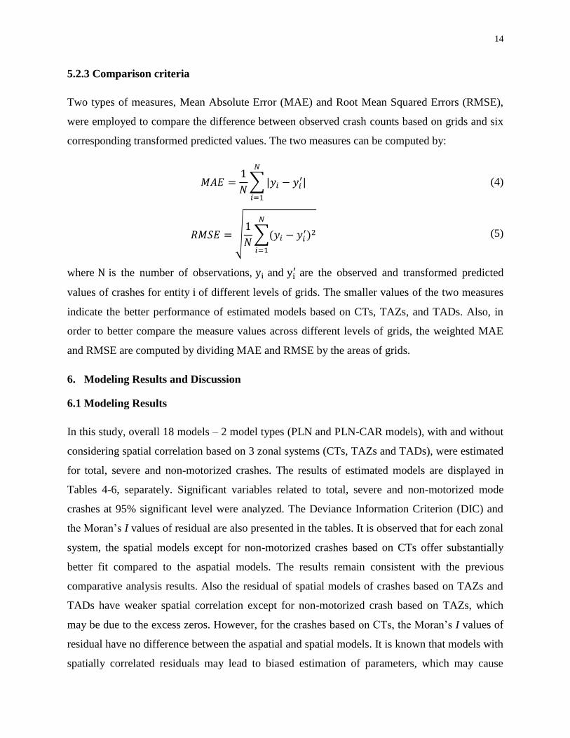
Modeling results for severe crashes for the three geographic units are summarized in Table 5.

The VMT and length of sidewalks are still significant in the three models. Higher median

household income results in decreased severe crashes for TAZs and TADs. Also proportion of

unemployment and proportion of commuters by public transportation are found significant in

CTs and TAZs. Finally, various variables such as proportion of heavy vehicle mileage in VMT,

roadway density, proportion of length of arterials and length of bike lanes are significant solely

in the TAZs based model.

16

6.1.3 Non-motorized Mode Crash

The results of the non-motorized mode crashes are shown in Table 6. The models based on the

three geographic units have expected variables such as VMT, proportion of heavy vehicle in

VMT, length of local roads, length of sidewalks, population density, commuters by public

transportation and cycling. As mentioned above, the VMT, a measure of vehicular exposure, is

expected to have positive impact on non-motorized mode crashes frequency. However, the

proportion of heavy vehicle VMT has a negative impact since the likelihood of non-motorists

drops substantially in the zones with increase in heavy vehicle VMT. The variables proportion of

local roads by length and length of sidewalks are reflections of pedestrian access and are likely to

increase crash frequency (Cai et al., 2016). The population density is a surrogate measure of non-

motorists exposure and is likely to increase the propensity for non-motorized mode crashes.

Across the three geographic units, it is observed that the zones with higher proportion of

commuters by public transportation and cycling have higher propensity for non-motorized mode

crashes. The commuters by public transportation and cycling are indications of zones with higher

non-motorists activity resulting in increased non-motorized mode crash risk (Abdel-Aty et al.,

2013).

17

Table 4. Total crash model results by zonal systems

Zonal systems CT TAZ TAD

Variables PLN PLN-CAR PLN PLN-CAR PLN PLN-CAR

Mean S.D. Mean S.D. Mean S.D. Mean S.D. Mean S.D. Mean S.D.

Intercept 1.163 0.026 0.751 0.078 3.35 0.044 1.187 0.057 -1.554 0.023 -0.155 0.689

(1.119, 1.207) (0.589, 0.911) (3.285, 3.409) (1.066, 1.274) (-1.591, -1.511) (-1.674, 1.255)

Log (VMT) 0.261 0.002 0.271 0.006 0.22 0.013 0.287 0.006 0.655 0.001 0.754 0.024

(0.257, 0.264) (0.261, 0.282) (0.199, 0.240) (0.275, 0.302) (0.654, 0.656) (0.713, 0.800)

Proportion of heavy vehicle mileage in VMT

- - - - -2.189 0.29 -1.532 0.355 -2.32 0.322 -4.009 0.457

- - (-2.655, -1.497) (-2.202, -0.904) (-2.798, -1.796) (-4.819, -2.953)

Log (signalized intersection density)

- - - - - - - - 0.579 0.056 0.685 0.162

- - - - (0.455, 0.682) (0.203, 0.971)

Log (length of sidewalks) 0.331 0.007 0.342 0.017 0.495 0.047 0.519 0.022 0.085 0.006 0.082 0.01

(0.316, 0.345) (0.297, 0.379) (0.383, 0.546) (0.475, 0.573) (0.075, 0.095) (0.061, 0.101)

Log (distance to nearest urban area)

- - - - -0.513 0.023 -0.181 0.027 - - - -

- - (-0.560, -0.479) (-0.274, -0.109) - -

Log (population density) - - - - - - - - 0.168 0.002 0.083 0.006

- - - - - - - - (0.163, 0.171) (0.071, 0.097)

Proportion of population age 15-24

- - 0.733 0.16 - - - - - - - -

- (0.398, 1.076) - - - -

Proportion of population age 65 or older

-1.469 0.056 -1.07 0.087 -1.079 0.206 -0.003 0.001 - - - -

(-1.560, -1.350) (-1.234, -0.893) (-1.354, -0.608) (-0.006, -0.001) - -

Proportion of unemployment - - - - -1.505 0.082 - - - - - -

- - (-1.680, -1.380) - - -

Log (Commuters density) 0.144 0.002 0.167 0.006 - - - - - - - -

(0.140, 0.148) (0.154, 0.180) - - - -

Proportion of commuters by public transportation

2.778 0.231 2.486 0.285 2.422 0.413 - - 5.464 0.312 2.427 0.995

(2.376, 3.230) (1.834, 2.996) (1.929, 3.257) - (4.975, 6.146) (0.432, 4.378)

Proportion of commuters by walking

1.06 0.231 - - - - - - - - - -

(0.698, 1.634) - - - - -

Log (median household income)

- - - - -0.06 0.004 - - -0.123 0.002 -0.301 0.063

- - (-0.068, -0.054) - (-0.126, -0.123) (-0.419, -0.160)

S.D. of θ 0.695 0.003 0.339 0.064 1.033 0.006 0.378 0.04 0.388 0.001 0.136 0.01

(0.691, 0.702) (0.241, 0.519) (1.024, 1.046) (0.308, 0.467) (0.385, 0.391) (0.117, 0.154)

S.D. of φ - - 0.213 0.028 - - 0.393 0.083 - - 0.14 0.011

- (0.166, 0.275) - (0.306, 0.591) - (0.118, 0.161)

DIC 36898.300 36854.800 64441.000 64147.960 6446.200 6435.659

Moran’s I of residual* 0.053 0.006 0.460 -0.020 0.412 -0.153

*All explanatory variables are significant at 95% confidence level; All Moran’s I values are significant at 95% confidence level

18

Table 5. Severe crash model results by zonal systems

Zonal systems CT TAZ TAD

Variables PLN PLN-CAR PLN PLN-CAR PLN PLN-CAR

Mean S.D. Mean S.D. Mean S.D. Mean S.D. Mean S.D. Mean S.D.

Intercept -2.493 0.094 -1.57 0.097 -1.344 0.069 -1.745 0.127 2.137 0.101 2.92 0.749

(-2.704, -2.376) (-1.768, -1.379) (-1.466, -0.217) (-2.024, -1.466) (1.971, 2.279) (1.375, 4.447)

Log (VMT) 0.402 0.007 0.339 0.009 0.364 0.005 0.33 0.007 0.591 0.01 0.529 0.025

(0.388, 0.418) (0.322, 0.357) (0.354, 0.371) (0.318, 0.345) (0.576, 0.606) (0.476, 0.583)

Proportion of heavy vehicle

mileage in VMT

- - - - -2.383 0.277 -0.935 0.300 -1.671 0.349 - -

- - (-2.908, -1.859) (-1.570, -0.312) (-2.391, -1.098) -

Log (roadway density) - - - - -0.024 0.011 -0.108 0.016 - - - -

- - (-0.050, -0.003) (-0.140, -0.076) - -

Proportion of length of

arterials

- - - - -0.604 0.044 -0.591 0.045 - - - -

- - (-0.686, -0.518) (-0.678, -0.502) - -

Proportion of length of

collectors

- - -0.283 0.083 - - - - - - - -

- (-0.452, -0.123) - - - -

Proportion of length of local

roads

0.263 0.043 - - - - - - 0.851 0.076 - -

(0.184, 0.352) - - - (0.701, 0.989) -

Log (length of bike lanes) - - - - 0.082 0.028 0.113 0.028 - - - -

- - (0.026, 0.134) (0.061, 0.166) - -

Log (length of sidewalks) 0.183 0.016 0.238 0.018 0.245 0.024 0.354 0.021 0.116 0.02 0.104 0.018

(0.154, 0.214) (0.203, 0.273) (0.187, 0.282) (0.313, 0.393) (0.084, 0.151) (0.068, 0.141)

Log (distance to nearest urban

area)

- - 0.201 0.018 - - - - - - - -

- (0.168, 0.238) - - - -

Proportion of unemployment -0.222 0.07 -0.444 0.081 -0.766 0.079 -0.152 0.089 - - - -

(-0.343, -0.063) (-0.605, -0.278) (-0.935, -0.614) (-0.330, 0.032) - -

Proportion of commuters by

public transportation

1.423 0.268 1.554 0.269 1.724 0.256 1.015 0.33 - - - -

(0.862, 1.934) (1.032, 2.048) (1.244, 2.206) (0.423, 1.670) - -

Proportion of commuters by

walking

0.976 0.273 - - - - - - - - - -

(0.450, 1.525) - - - - -

Log (median household

income)

- - - - -0.037 0.003 -0.021 0.009 -0.589 0.007 -0.536 0.062

- - (-0.043, -0.030) (-0.039, -0.004) (-0.604, -0.576) (-0.659, -0.412)

S.D. of θ 0.614 0.007 0.218 0.049 0.835 0.008 0.393 0.045 0.458 0.006 0.116 0.006

(0.601, 0.628) (0.166, 0.329) (0.819, 0.852) (0.304, 0.470) (0.447, 0.469) (0.107, 0.129)

S.D. of φ - - 0.191 0.025 - - 0.519 0.024 - - 0.152 0.02

- (0.148, 0.247) - (0.278, 0.749) - (0.123, 0.199)

DIC 23958.000 23835.000 38158.200 37470.090 4741.080 4696.724

Moran’s I of residual 0.065 -0.007 0.397 0.040 0.370 -0.096

*All explanatory variables are significant at 95% confidence level; * All Moran’s I values are significant at 95% confidence level

19

Table 6. Non-motorized mode crash model results by zonal systems

Zonal systems CT TAZ TAD

Variables PLN PLN-CAR PLN PLN-CAR PLN PLN-CAR

Mean S.D. Mean S.D. Mean S.D. Mean S.D. Mean S.D. Mean S.D.

Intercept -2.539 0.062 -2.256 0.129 -3.612 0.157 -3.503 0.144 0.176 0.063 4.737 1.221

(-2.664, -2.388) (-2.510, -1.996) (-3.812, -3.301) (-3.800, -3.200) (0.069, 0.285) (2.412, 7.038)

Log (VMT) 0.172 0.007 0.161 0.008 0.297 0.005 0.283 0.007 0.345 0.004 0.252 0.038

(0.161, 0.186) (0.145, 0.177) (0.289, 0.307) (0.268, 0.298) (0.336, 0.352) (0.179, 0.331)

Proportion of heavy

vehicle mileage in VMT

-1.858 0.330 -2.262 0.389 -4.389 0.432 -4.803 0.391 -3.639 0.440 -2.969 0.854

(-2.459, -1.134) (-3.053, -1.478) (-5.083, -3.520) (-5.518, -4.068) (-4.548, -2.884) (-4.519.-1.511)

Log (roadway density) - - - - 0.154 0.016 0.143 0.020 - - - -

- - (0.128, 0.189) (0.106, 0.182) - -

Proportion of length of

local roads

0.377 0.043 0.367 0.061 0.717 0.044 0.752 0.047 0.679 0.101 - -

(0.279, 0.453) (0.245, 0.488) (0.623, 0.794) (0.661, 0.845) (0.517, 0.838) -

Log (length of sidewalks) 0.48 0.017 0.488 0.019 0.506 0.022 0.558 0.022 0.283 0.015 0.306 0.027

(0.450, 0.516) (0.454, 0.524) (0.458, 0.545) (0.516, 0.602) (0.257, 0.315) (0.252, 0.360)

Log (population density) 0.243 0.005 0.225 0.010 0.234 0.006 0.175 0.010 0.22 0.009 0.165 0.024

(0.234, 0.252) (0.206, 0.247) (0.225, 0.246) (0.158, 0.192) (0.205, 0.237) (0.125, 0.215)

Proportion of population

age 65 or older

-0.691 0.098 -0.761 0.094 - - - - - - - -

(-0.890, -0.519) (-0.947, -0.582) - - - -

Log (Commuters

density)

- - - - -0.635 0.075 -0.398 0.099 - - - -

- - (-0.766, -0.450) (-0.587, -0.199) - -

Proportion of

commuters by public

transportation

3.532 0.260 3.565 0.292 3.467 0.258 2.949 0.282 7.525 0.606 4.802 1.286

(3.011, 4.049) (3.011, 4.102) (2.919, 3.974) (2.375, 3.457) (6.544, 8.900) (2.676, 7.015)

Proportion of

commuters by cycling

3.955 0.492 3.892 0.441 1.078 0.471 - - 7.000 1.703 8.566 2.258

(2.901, 4.918) (3.069, 4.792) (0.076, 1.960) - (4.180, 10.670) (3.955, 12.758)

Proportion of

commuters by walking

2.476 0.329 2.595 0.306 1.877 0.280 1.757 0.294 - - - -

(1.874, 3.116) (1.998, 3.145) (1.321, 2.405) (1.189, 2.325) - -

Log (median household

income)

- - - - -0.075 0.014 -0.047 0.01 -0.336 0.005 -0.565 0.094

- - (-0.098, -0.056) (-0.066, -0.026) (-0.344, 0.326) (-0.745, -0.384)

S.D. of θ 0.605 0.009 0.361 0.090 0.790 0.011 0.518 0.144 0.456 0.008 0.222 0.023

(0.588, 0.622) (0.196, 0.531) (0.769, 0.814) (0.224, 0.715) (0.440, 0.472) (0.181, 0.263)

S.D. of φ - - 0.053 0.008 - - 0.037 0.058 - - 0.198 0.028

- (0.042, 0.072) - (0.010, 0.152) - (0.147, 0.261)

DIC 21032.300 21033.730 30244.700 29926.930 4317.540 4302.187

Moran’s I of residual 0.028 0.021 0.286 0.325 0.092 -0.088

*All explanatory variables are significant at 95% confidence level; * All Moran’s I values are significant at 95% confidence level

20

6.2 Comparative Analysis Results

Based on the estimated models of the three zonal systems, the predicted crash counts for each

crash type of the three geographic units can be computed and then transformed into the

correspondingly intersected grids. Weighted MAE and RMSE for each grid structure were

calculated with the observed crash counts and transformed predicted crash counts based on

different geographic units. The comparison results are as shown in Table 7 and several

observations can be made. (1) The MAE and RMSE values consistently increase with the grid

size, validating the previous discussion that the comparison measures can be influenced by the

number of observations and observed values. (2) For each zonal system, the spatial (PLN-CAR)

models substantially improve the performance over the aspatial (PLN) models for predicting

crash counts. The results are consistent with the previous analysis results that the crash counts

are spatially correlated and the model considering the spatial dependency can provide better

understanding of crash frequency. Also, the improvements based on TAZs and TADs are much

greater than that based on CTs which should be related to the spatial correlation levels. (3)

Among aspatial and spatial models, the TADs always have the best performance indicating the

advantages of TADs over the other two zonal systems. Meanwhile, CTs based on aspatial models

can consistently perform better than the models based on TAZs. However, the exact ordering

alters between spatial models based on CTs and TAZs according to MAE and RMSE.

The CTs are designed to be comparatively homogenous units with respect to socio-demographic

statistical data. Thus, it is not surprising that CT-based models do not show the best performance.

TAZs are the base zonal system of analyses for developing travel demand models and have been

widely used by metropolitan planning organizations for their long range transportation plans.

However, one of the major zoning criteria for TAZs is to minimize the number of intra-zonal

trips (Meyer & Miller, 2001) which results in small area size for each TAZ. Due to the small size,

a crash occurring in a TAZ might be caused by the driver from another TAZ, i.e., the

characteristics of drivers who cause the crashes cannot be observed by the models based on

TAZs. Also, as TAZs are often delineated by arterial roads and many crashes occur on these

boundaries. The existence of boundary crashes may invalidate the assumptions of modeling only

based on the characteristics of a zone where the crash is spatially located (Lee et al, 2014;

Siddiqui et al., 2012). Hence, although TAZs are appropriate for transportation demand

21

forecasting, they might be not the best option for the transportation safety planning. The TADs

are another transportation-related zonal system with considerably larger size compared with

TAZs. There should be more intra-zonal trips in each TAD and the drivers who cause crashes in

a TAD will be more likely to come from the same TAD. So it seems reasonable that TADs are

superior for macro-level crash analysis and transportation safety planning.

In summary, considering the rationale for the development of different zonal systems and the

modeling results in our study, it is recommended using CTs for socio-demographic data

collection, employing TAZs for transportation demand forecasting, and adopting TADs for

transportation safety planning.

22

Table 7. Comparison results based on grids

Total Crashes Severe Crashes Non-motorized Crashes

PLN PLN_CAR PLN PLN_CAR PLN PLN_CAR

CT TAZ TAD CT TAZ TAD CT TAZ TAD CT TAZ TAD CT TAZ TAD CT TAZ TAD

Weighted MAE

Grid 1×1 4.70 6.12 3.43 4.45 3.34 2.30 0.28 0.33 0.22 0.26 0.23 0.18 0.17 0.19 0.15 0.17 0.18 0.12

Grid 2×2 4.22 5.61 3.25 3.95 2.62 2.03 0.25 0.30 0.21 0.23 0.19 0.15 0.14 0.17 0.14 0.14 0.16 0.11

Grid 3×3 3.87 5.23 3.10 3.59 2.19 1.85 0.23 0.28 0.20 0.21 0.17 0.14 0.13 0.16 0.13 0.13 0.15 0.10

Grid 4×4 3.63 4.97 3.01 3.36 1.93 1.61 0.21 0.26 0.20 0.19 0.15 0.12 0.12 0.15 0.12 0.12 0.14 0.09

Grid 5×5 3.42 4.74 2.79 3.16 1.81 1.39 0.20 0.25 0.19 0.18 0.14 0.10 0.11 0.14 0.11 0.11 0.13 0.08

Grid 6×6 3.30 4.57 2.72 3.03 1.65 1.20 0.19 0.24 0.19 0.17 0.14 0.10 0.10 0.14 0.10 0.10 0.12 0.07

Grid 7×7 3.18 4.43 2.68 2.94 1.55 1.17 0.18 0.23 0.18 0.17 0.13 0.09 0.10 0.13 0.10 0.10 0.12 0.07

Grid 8×8 3.06 4.31 2.58 2.82 1.49 1.08 0.18 0.23 0.17 0.16 0.13 0.08 0.09 0.13 0.09 0.09 0.11 0.06

Grid 9×9 2.99 4.23 2.53 2.74 1.47 0.94 0.17 0.22 0.17 0.15 0.12 0.07 0.09 0.13 0.09 0.09 0.11 0.06

Grid 10×10 2.84 4.08 2.41 2.60 1.38 0.94 0.16 0.21 0.17 0.15 0.12 0.07 0.09 0.12 0.08 0.09 0.11 0.05

AVE 3.52 4.83 2.85 3.26 1.94 1.45 0.21 0.25 0.19 0.19 0.15 0.11 0.11 0.15 0.11 0.11 0.13 0.08

Weighted RMSE

Grid 1×1 31.84 39.77 27.82 29.41 20.54 19.56 1.40 1.66 1.31 1.35 1.07 1.11 1.12 1.37 1.49 1.11 1.22 1.33

Grid 2×2 25.54 32.53 22.64 23.27 12.60 14.61 1.07 1.30 1.02 1.03 0.73 0.74 0.77 0.96 1.00 0.76 0.85 0.87

Grid 3×3 22.38 28.99 18.89 20.19 9.31 11.23 0.91 1.13 0.88 0.87 0.57 0.67 0.62 0.79 0.81 0.62 0.70 0.61

Grid 4×4 20.30 26.18 16.78 18.16 7.68 7.65 0.83 1.04 0.80 0.79 0.51 0.55 0.54 0.72 0.59 0.54 0.64 0.46

Grid 5×5 19.53 25.41 16.06 17.54 6.53 7.28 0.73 0.95 0.70 0.70 0.44 0.34 0.48 0.66 0.57 0.48 0.57 0.43

Grid 6×6 18.30 23.92 15.10 16.34 5.50 5.25 0.66 0.86 0.65 0.61 0.39 0.31 0.44 0.60 0.48 0.43 0.52 0.35

Grid 7×7 17.43 22.58 14.72 15.46 4.81 5.51 0.58 0.79 0.59 0.55 0.34 0.25 0.39 0.54 0.40 0.39 0.46 0.27

Grid 8×8 17.43 22.65 14.24 15.41 4.68 4.86 0.59 0.79 0.58 0.55 0.35 0.24 0.36 0.52 0.38 0.36 0.44 0.25

Grid 9×9 16.10 21.23 12.85 14.23 4.35 3.56 0.53 0.73 0.54 0.50 0.32 0.22 0.35 0.51 0.35 0.35 0.43 0.21

Grid 10×10 15.45 21.18 12.79 13.71 3.89 4.03 0.49 0.71 0.49 0.47 0.31 0.17 0.32 0.50 0.31 0.32 0.40 0.18

AVE 20.43 26.44 17.19 18.37 7.99 8.35 0.78 0.99 0.76 0.74 0.50 0.46 0.54 0.72 0.64 0.54 0.62 0.50

23

7. Conclusion

Macro-level safety modeling is one of the important objectives in transportation safety planning.

Although various geographic units have been employed for macro-level crash analysis, there has

been no guidance to choose an appropriate zonal system. One of difficulties is to compare

models based on different geographic units of which number of zones is not the same. This study

proposes a new method for the comparison between different zonal systems by adopting grid

structures of different scales. The Poisson lognormal (PLN) models without and Poisson

lognormal conditional autoregressive model (PLN-CAR) with consideration of spatial

correlation for total, severe, and non-motorized mode crashes were developed based on census

tracts (CTs), traffic analysis zones (TAZs), and a newly developed traffic-related zone system -

traffic analysis districts (TADs). Based on the estimated models, predicted crash counts for the

three zonal systems were computed. Considering the average area of each geographic unit, ten

sizes of grid structures with dimensions ranging from 1 mile to 100 square miles were created for

the comparison of estimated models. The observed crash counts for each grid were directly

obtained with GIS while the different predicted crash counts were transformed into the grids that

each geographic unit intersects with. The weighted MAE and RMSE were calculated for the

observed and different transformed crash counts of different grid structures. By comparing the

MAE and RMSE values, the best zonal system as well as model for macroscopic crash modeling

can be identified with the same sample size.

The comparison results indicated that the models based on TADs offered the best fit for all crash

types. Based on the modeling results and the motivation for developing the different zonal

systems, it is recommended CTs for socio-demographic data collection, TAZs for transportation

demand forecasting, and TADs for transportation safety planning. Also, the comparison results

highlighted that models with the consideration of spatial effects consistently performed better

than the models that did not consider the spatial effects. The modeling results based on different

zonal systems had different significant variables, which demonstrated the zonal variation.

Besides, the results clearly highlighted the importance of several explanatory variables such as

traffic (i.e., VMT and heavy vehicle mileage), roadway (e.g., proportion of local roads in length,

signalized intersection density, and length of sidewalks, etc.) and socio-demographic

characteristics (e.g., population density, commuters by public transportation, walking as well as

cycling, median household income, and etc.).

24

This study focuses on the comparison of zonal systems for crash modeling and transportation

safety planning. However, only three zonal systems were adopted for the validation of the

proposed comparison method. Extending the current approach to compare other zonal systems

(e.g., census block and counties) could be meaningful. Also, it is possible that the trip distance

might be related to the size of appropriate geographic units for crash modeling. Future research

extension might consider such relationship.

ACKNOWLEDGMENT

The authors would like to thank the Florida Department of Transportation (FDOT) for funding

this study.

REFERENCE

Abdel-Aty, M., Lee, J., Siddiqui, C., & Choi, K. (2013). Geographical unit based analysis in the

context of transportation safety planning. Transportation Research Part A: Policy and Practice 49,

62-75.

Abdel-Aty, M., Siddiqui, C., & Huang, H. (2011). Integrating Trip and Roadway Characteristics

in Managing Safety at Traffic Analysis Zones. Compendium of papers CD-ROM, Transportation

Research Board 90th Annual Meeting, Washington, D.C.

Aguero-Valverde, J., & Jovanis, P.P. (2006). Spatial analysis of fatal and injury crashes in

Pennsylvania. Accident Analysis & Prevention 38, 618-625.

Anselin, L. (2013). Spatial econometrics: methods and models. Springer Science & Business

Media.

Besag, J., York, J., & Mollié, A. (1991). Bayesian image restoration, with two applications in

spatial statistics. Annals of the institute of statistical mathematics 43, 1-20.

Cai, Q., Lee, J., Eluru, N., & Abdel-Aty, M. (2016). Macro-level pedestrian and bicycle crash

analysis: incorporating spatial spillover effects in dual state count models. Accident Analysis &

Prevention 93, 14-22.

FHWA, Census Transportation Planning Products (CTPP). (2011). 2010 census traffic analysis

zone program MAF/TIGER partnership software participant guidelines.

Hadayeghi, A., Shalaby, A., & Persaud, B. (2003). Macrolevel accident prediction models for

evaluating safety of urban transportation systems. Transportation Research Record: Journal of

the Transportation Research Board, 87-95.

Hadayeghi, A., Shalaby, A.S., & Persaud, B.N. (2010). Development of planning level

transportation safety tools using geographically weighted Poisson regression. Accident Analysis

& Prevention 42, 676-688.

25

Huang, H., Abdel-Aty, M., & Darwiche, A. (2010). County-level crash risk analysis in Florida:

Bayesian spatial modeling. Transportation Research Record: Journal of the Transportation

Research Board, 27-37.

Kim, K., Brunner, I., & Yamashita, E. (2006). Influence of land use, population, employment,

and economic activity on accidents. Transportation Research Record: Journal of the

Transportation Research Board, 56-64.

Ladrón de Guevara, F., Washington, S., & Oh, J. (2004). Forecasting crashes at the planning

level: simultaneous negative binomial crash model applied in Tucson, Arizona. Transportation

Research Record: Journal of the Transportation Research Board, 191-199.

LaScala, E.A., Gerber, D., & Gruenewald, P.J. (2000). Demographic and environmental

correlates of pedestrian injury collisions: a spatial analysis. Accident Analysis & Prevention 32,

651-658.

Lee, J., Abdel-Aty, M., Choi, K., & Siddiqui, C. (2013). Analysis of residence characteristics of

drivers, pedestrians, and bicyclists involved in traffic crashes, Compendium of papers CD-ROM,

Transportation Research Board 92nd Annual Meeting, Washington, D.C.

Lee, J., Abdel-Aty, M., & Jiang, X. (2014). Development of zone system for macro-level traffic

safety analysis. Journal of transport geography 38, 13-21.

Lee, J., Abdel-Aty, M., Choi, K., & Huang, H. (2015). Multi-level hot zone identification for

pedestrian safety. Accident Analysis & Prevention 76, 64-73.

Levine, N., Kim, K.E., & Nitz, L.H. (1995). Spatial analysis of Honolulu motor vehicle crashes:

I. Spatial patterns. Accident Analysis & Prevention 27, 663-674.

Lord, D., & Mannering, F. (2010). The statistical analysis of crash-frequency data: a review and

assessment of methodological alternatives. Transportation Research Part A: Policy and Practice

44, 291-305.

Meyer, M.D., & Miller, E.J. (2001). Urban Transportation Planning: A Decision-oriented

Approach. 2nd edition. McGraw-Hill, New York.

Meyer, M.D., Systematics, C., & Association, A.A. (2008). Crashes Vs. Congestion: What's the

Cost to Society? American Automobile Association.

Quddus, M.A. (2008). Modelling area-wide count outcomes with spatial correlation and

heterogeneity: an analysis of London crash data. Accident Analysis & Prevention 40, 1486-1497.

Siddiqui, C., & Abdel-Aty, M. (2012). Nature of modeling boundary pedestrian crashes at zones.

Transportation Research Record: Journal of the Transportation Research Board, 31-40.

Wang, Y., & Kockelman, K.M. (2013). A Poisson-lognormal conditional-autoregressive model

for multivariate spatial analysis of pedestrian crash counts across neighborhoods. Accident

Analysis & Prevention 60, 71-84.

Xu, P., Huang, H., Dong, N., & Abdel-Aty, M. (2014). Sensitivity analysis in the context of

regional safety modeling: Identifying and assessing the modifiable areal unit problem. Accident

Analysis & Prevention 70, 110-120.

26

Yasmin, S., & Eluru, N. (2016). Latent Segmentation Based Count Models: Analysis of Bicycle

Safety in Montreal and Toronto. Accident Analysis & Prevention 95, 157-171.