Comparative Analysis of the Quantization of Color Spaces on the

Comparative Analysis of the Quantizationof Color Spaces on the Basis of theCIELAB Color-Difference Formula

B. HILL, Th. ROGER, and F. W. VORHAGENAachen University of Technology

This article discusses the CIELAB color space within the limits of optimal colors including thecomplete volume of object colors. A graphical representation of this color space is composed ofplanes of constant lightness L* with a net of lines parallel to the a* and b* axes. This uniformnet is projected onto a number of other color spaces (CIE XYZ, tristimulus RGB, predistortedRGB, and YCC color space) to demonstrate and study the structure of color differences inthese spaces on the basis of CIELAB color difference formulas. Two formulas are considered:the CIE 1976 formula DEab and the newer CIE 1994 formula DE*94. The various color spacesconsidered are uniformly quantized and the grid of quantized points is transformed intoCIELAB coordinates to study the distribution of color differences due to basic quantizationsteps and to specify the areas of the colors with the highest sensitivity to color discrimination.From a threshold value for the maximum color difference among neighboring quantized pointssearched for in each color space, concepts for the quantization of the color spaces are derived.The results are compared to quantization concepts based on average values of quantizationerrors published in previous work. In addition to color spaces bounded by the optimal colors,the studies are also applied to device-dependent color spaces limited by the range of a positiveRGB cube or by the gamut of colors of practical print processes (thermal dye sublimation,Chromalin, and Match Print). For all the color spaces, estimations of the number of distin-guishable colors are given on the basis of a threshold value for the color difference perceptionof DEab 5 1 and DE*94 5 1.

Categories and Subject Descriptors: G.1.2 [Numerical Analysis]: Approximation; I.3.1 [Com-puter Graphics]: Hardware Architecture; I.3.3 [Computer Graphics]: Picture/Image Gen-eration—display algorithms; I.3.7 [Computer Graphics]: Three-Dimensional Graphics andRealism—color, shading, shadowing, and texture; I.4.1 [Image Processing]: Digitization—quantization

General Terms: Algorithms, Experimentation, Performance, Standardization

Additional Key Words and Phrases: CIE XYZ, CIELAB, CIELAB color space, CIELUV, colordifference perception, color quantization, color spaces, Cromalin, dye sublimation printer,match print, optimal colors, RGB, YCC

Authors’ address: Aachen University of Technology, RWTH, Templergraben 55, Aachen 52056,Germany.Permission to make digital / hard copy of part or all of this work for personal or classroom useis granted without fee provided that the copies are not made or distributed for profit orcommercial advantage, the copyright notice, the title of the publication, and its date appear,and notice is given that copying is by permission of the ACM, Inc. To copy otherwise, torepublish, to post on servers, or to redistribute to lists, requires prior specific permissionand / or a fee.© 1997 ACM 0730-0301/97/0400–0109 $03.50

ACM Transactions on Graphics, Vol. 16, No. 2, April 1997, Pages 109–154.

1. INTRODUCTION

The CIELAB color space is one of the approximately uniform color spacesrecommended for device-independent color representation in electroniccolor image systems. Color as part of the information of a document isdescribed at less redundancy in CIELAB dimensions than in linear RGB orXYZ primary color systems and it has therefore been introduced intoPostscript language and Photoshop and is increasingly used and acceptedin all kinds of professional and commercial imaging systems for colorrepresentation.

If colors are represented by the CIELAB space, the axes of lightness L*and chromaticities a* and b* have to be suitably quantized. Therefore therange of colors and the limitations of the axes have to be specified. Thestandardized CIELAB definition [CIE 1986a] gives a limit only for the L*axis (0 # L* # 100) whereas no limitations are specified for a* and b*. Asfar as object colors are concerned, a theoretical limitation is given by theso-called optimal colors derived from the limited spectral reflectance ortransmission curves together with a specified illuminant [Schrodinger1920; Rosch 1929; MacAdam 1935a, b]. A color space with the surface ofoptimal colors includes all the smaller color gamuts in technical reproduc-tions.

The primary aim of this article is to describe the gamut of optimal colorsin a specified grid of the CIELAB space and to make evident how thisgamut and grid of colors represents itself if it is transformed into a numberof other typical color spaces. Therefore the CIELAB optimal color space[CIE 1986b], the CIE XYZ [CIE 1986c], the RGB [CCIR 1982], and theKodak YCC color spaces [Kodak 1992] with the gamut of optimal colors arerepresented in graphical form.

These representations also show clearly the principal structure of theCIELAB space compared to other color spaces. If cells of cubic form invarious parts of the CIELAB space are transformed into other color spacessuch as the XYZ or RGB space, they become deformed and in some casesstrongly compressed. These deformations demonstrate the differing sensi-tivities of color perception as a function of the coordinates among thedifferent color spaces and within each color space.

The colors in technical reproduction systems cover a smaller gamut thanthose of optimal colors. To demonstrate the typical differences, the tris-timulus and predistorted RGB space with positive components between 0and 100 only (ITU-R BT.709, formerly CCIR 709), the Kodak YCC spacewith standard specification [Kodak 1992], and the device-dependent colorspaces of a thermal dye sublimation printer, and the Chromalin proofingsystem are presented in CIELAB coordinates.

A last aim of this article is to compare the quantization of the variouscolor spaces examined. Therefore the same quantization concept is appliedto the various color spaces without matching the quantization to a specialapplication. This has the advantage that specific differences among thecolor spaces can be exposed. The quantization is based on the CIELAB color

110 • B. Hill et al.

ACM Transactions on Graphics, Vol. 16, No. 2, April 1997.

difference formulas. The most common formula was published in 1976 [CIE1986a]. An improved formula was recommended by the CIE TechnicalCommittee 1-29 in 1994 [Alman 1993; CIE 1993]. Both formulas are usedas a basis for quantization and we outline the essential differences result-ing from the different structures of the formulas.

Quantization concepts have already been discussed in other papers. InKasson and Plouffe [1992], a number of test colors within the range of realsurface colors as given by Pointer [1980] are defined for three levels oflightness in the CIELUV space. An arbitrary number of sample pointsaround the test points defines shifted colors used to calculate small colordifferences. These points are then transformed into a color space to bestudied and they are quantized in this space assuming an 8-bit quantiza-tion per axis. Then the quantized points are transformed back into thesource color space and compared with the exact points not being quantized.The resulting differences provide transformed quantization errors. Fromthese, an average error over all the test points and the statistical three-sigma error is calculated in terms of the CIELUV—as well as theCIELAB—color difference definitions DEuv and DEab. The result of theaverage error is finally expressed as the average value from both colordifference definitions, whereas the maximum of both is used for theaverage three-sigma error. As a typical result, the quantization of 8 1 8 18 bits yields an average three-sigma error of 0.5 for the quantization of theCIELUV space, 0.4 for the CIELAB space, and 4.1 for the CIE XYZ space,respectively. Reduction of the error by a factor of 2 requires approximately1 bit more per component, which means, for example, that 10 bits percomponent are necessary to come to an error close to DE 5 1 for thequantization of the CIE XYZ space.

An experimental method to estimate a useful quantization was publishedin Stokes et al. [1992a]. Perceptibility experiments at pictorial imagesreproduced on a high quality display were performed to derive perceptibil-ity tolerances expressed in DEab units. A variety of typical color manipula-tions was applied to a large number of images of different types. Finally, anaverage perceptibility threshold of DEab 5 2.15 was found. From thisresult, the minimum quantization of 6.4 bits for the L* axis and 7.1 bits forthe a* and b* axes of the CIELAB space are specified. For the quantizationof a nonlinear RGB CRT color space, 7.4 bits per component are derived.

In Mahy et al. [1991], quantization errors in an RGB color space for an8-bit quantization have been calculated and transformed into CIELAB,CIELUV, and ATD color spaces. Maximum and mean errors are outlinedfor grey values (equal components of RGB). Large differences among theerrors were found for high and low grey values and among the differentcomponents of the color spaces. From experiments with displayed images, aperceptable threshold value of DEab 5 1 was found for the lightness and 3for chroma values a* and b*.

In this article, maximum color quantization steps of a number of colorspaces instead of mean errors are calculated for all possible directions ofquantized steps in three-dimensional spaces and for all the positions within

Quantization of Color Spaces • 111


each space. Maximum color quantization steps provide a “worst case” basisfor the estimation of necessary quantization concepts. Those concepts areoutlined for the CIELAB, CIELUV, and CIE XYZ device-independent colorspaces and the tristimulus and predistorted RGB space (ITU-R BT.709,formerly CCIR 709) within the limits of optimal colors [MacAdam 1935a, b]and for tristimulus and predistorted RGB spaces with positive componentsbetween 0 and 100 only, for the Kodak YCC space [Kodak 1992] and fordevice-dependent color spaces of a thermal dye sublimation printer and theChromalin proofing system.

2. GENERAL CONCEPT OF THE ANALYSIS

2.1 CIELAB Color Space and Color Difference Formulas

The CIELAB system is a simplified mathematical approximation to auniform color space composed of perceived color differences. The perceivedlightness L* of a standard observer is assumed to follow the intensity of acolor stimulus according to a cubic root law [CIE 1986a]. The colors oflightness L* are arranged between the opponent colors green-red andblue-yellow along the rectangular coordinates a* and b*. The total differ-ence between the two colors is given in terms of L*, a*, b* by the CIE 1976formula

DEab 5 ÎDL*2

1 Da*2

1 Db*2

.

Any color represented in the rectangular coordinate system of axes L*, a*,b* can alternatively be expressed in terms of polar coordinates with theperceived lightness L* and the psychometric correlates of chroma,

Cab* 5 Îa*2

1 b*2

,

and hue angle,

hab 5 tan21S b*

a*D .

In fact, the CIELAB space is not really uniform. If MacAdam or Brown-MacAdam ellipses or ellipsoids are transformed into CIELAB coordinates,differences appear among their main axes of up to 1:6.

In particular, at high values of chroma, the simple CIE 1976 colordifference formulas value color differences too strongly compared to exper-imental results of color perception [Loo and Rigg, 1987]. An improved colordifference formula was therefore recommended in 1994 [Alman 1993; CIE1993, 1995]:

DE*94 5 ÎS DL*

kLSLD 2

1 SDC*ab

kCSCD 2

1 SDH*ab

kHSHD 2

,



where DL*, DC*ab, and DH*ab are the CIELAB 1976 color differences oflightness, chroma, and hue; kL, kC, and kH are factors to match theperception of background conditions; and SL, SC, and SH are linear func-tions of C*ab. Color differences in this article have also been calculated forthis formula and they are compared to the calculations for DEab. Standardreference values as specified in CIE [1993, 1995] have been assumed for thecalculations of DE*94:

kL 5 kC 5 kH 5 1, SL 5 1

SC 5 1 1 0.045 C*ab, SH 5 1 1 0.015 C*ab.

2.2 CIELAB Optimal Color Space

The volume of all the object colors that appear in nature is enclosed by theoptimal colors with maximum saturation for a given lightness (Figure 1). Acolor space with the surface of the optimal colors therefore includes all thesmaller gamuts of colors in technical reproductions using reflective ortransmissive materials under a given illuminant [Schrodinger 1920; Rosch1929; MacAdam 1935a, b].

Not included in the theory of color limitation by optimal colors areself-luminous colors. Nevertheless, the self-luminous colors of displays orother image sources can be included in a color space with the surface ofoptimal colors (hereafter called “optimal color space”), if the averagelightness is clearly specified and matched to the average lightness of thesurrounding scene. If, however, self-luminous colors are combined withreflective or transmissive colors in the same document, it has to be checkedcarefully whether the resulting colors are still represented in an optimalcolor space. Many printing papers with luminescent additions are problem-atic in this respect.

A comprehensive study of the gamut of colors has been given by Pointer[1980]. Film colors as well as real surface colors and their limits ofmaximum saturation are derived from experimental data and color books.As far as optimal colors are concerned, it has been proposed to use so-called“reduced optimal colors” instead of the theoretical values to take the finiteoptical density of reflective colors into account. This density is alwayslimited by reflection and scattering of light at the surface of color pigments.When considering a maximum optical density of D 5 2.25, the colors ofmaximum saturation are shifted by a few percent compared to the optimalcolors with the theoretical density of infinity. Although the optical densitylimit of 2.25 is realistic for many prints, the limitation is very different forphotographic transparencies and displays. To be independent of specifictechnologies, the absolute theoretical limits for optimal colors have beenused in this article.

The CIELAB optimal color space bounded by the surface of the mostsaturated colors is shown in Figure 2. The space is composed of planes ofconstant lightness L* that are arranged at distances of 5 units apart. Eachplane is limited by the optimal colors of the respective lightness.



The calculation of these color planes starts from a CIE Yi value accordingto a given lightness L*i. For type 1 optimal colors (see Figure 1), theequation

Yi~l j, Dl i, j! 5 K z Elj

lj1Dli, j

Sl z y~l!dl; K 5100

*380 nm780 nm Sl z y~l!dl

has to be solved as a function of Dli, j for each value of lj. The function y(l)is the spectral matching curve of the CIE XYZ system.

An equal-energy flux Sl 5 1 has been assumed for the calculation of thegeneral color spaces CIELAB and CIE XYZ, and Sl according to theilluminant D65 has been considered for specific color spaces in RGB or YCCcomponents. Starting from a specific value of the lightness L* transferredto Yi, the integral equation results in a value Dli, j for each value of lj. For

Fig. 1. Remission curves of a spectral object color (a), an optimal color type 1 (b), and anoptimal color type 2 (c). An optimal color is an object color with the spectral remissionoccupying only the two extreme values b(l) 5 1 or b(l) 5 0 and with, at a maximum, only twosteps between these values. Each optimal color is the most saturated color of given chromatic-ity at a given lightness. Two types of optimal colors are possible, one with the remission curveoccupying a continuous range Dl1 of the spectrum (type 1) and another occupying two separateranges (type 2) with single steps.



the results shown in Figure 2, the wavelength lj has been varied in steps of1 nm throughout the visible spectrum. The same procedure is applied totype 2 optimal colors as well. With the integration limits found, theaccompanying X and Z optimal color values are determined:

Xi, j 5 K z Elj

lj1Dli, j

Sl z x~l!dl, Zi, j 5 K z Elj

lj1Dli, j

Sl z z~l!dl.

All the results of color values Xi, j, Yi, and Zi, j are lined up for eachparticular value of Yi, interpolated, and converted to the L*, a*, b* valuesthat describe the border line of a plane L*i in Figure 2.

The optimal color space shows some typical characteristics. The lowerplanes are stretched out into the blue range forming a slim “nose.” Athigher lightness, the center of the planes moves from blue towards yellow.At low lightness, blue colors are dominant. At medium lightness, a maxi-mum number of perceivable colors is achieved and at high lightness, onlyyellow and green colors are present.

Figure 3 shows a top view of the CIELAB optimal color space for equalenergy flux Sl 5 1 according to the light source demonstrating the overalldimensions in the a*-, b*-plane. The CIELAB optimal color space is thusarrayed within the limits 0 # L* # 100; 2166 , a* , 141; 2132 , b* ,147.

Fig. 2. CIELAB optimal color space composed of planes of constant lightness L* spacedDL* 5 5 units. The net indicated in each plane represents lines of constant a* or b* with linespacings of 20 units.



2.3 CIELAB Color Difference Formula, Just-Noticeable Color Difference, andNumber of Bits

For quantizing color spaces, a threshold value of color differences has to bedefined. Although many studies have dealt with this problem, a clearthreshold definition has not been given up to now. A first problem is thatthe CIELAB space is not really uniform and that therefore the perceptionof color differences changes with the location of colors within the colorspace and with the direction in the color space.

Another problem is that the just-noticeable threshold depends on thekind of image and the ambient illumination. An extensive experimentalstudy on perceptibility tolerances of pictorial images reproduced on CRTshas shown that the average perceptible difference lies in the range ofDEab ' 1.57 to 2.56 [Stokes et al. 1992a]. On average, a color difference of

Fig. 3. Top view on the CIELAB optimal color space. The uppermost plane corresponds to thelightness of L* 5 95. L* 5 100 gives the white point.



DEab ' 1 would not be noticed in electronic images after these experi-ments. The experiments published in Mahy et al. [1991], Schwarz et al.[1987], and Stokes et al. [1992b] result in the same order of magnitude ofperceptibility thresholds between 1 and 3 for practical images. In profes-sional or electronic prints, the uncertainty of color reproduction is typicallyof the order of several units of DEab. On the other hand, color differencethresholds of much below DEab ' 1 are required in some fields of industrialcoloring, when comparing, for example, colors of cars or textiles [SAE1985]. In this article, thresholds of DE ' 1 or DE*94 ' 1 have been assumedas a worthwhile basis for quantization in view of the requirements inelectronic imaging. For complex computing of colors, it may be necessary touse lower quantization thresholds than for the reproduction of a finalimage because quantization errors add up in a series of calculations [Stokeset al. 1992b]. If required, the results derived in this article can beapproximately converted to lower or higher limits of the threshold of DEaccording to the relation that 1 bit more for all 3 color components reducesthe color quantization threshold by the factor 2 and vice versa. Thus theresults shown in this article can be matched to differing requirements ofpractical engineering problems. If a bit number is derived from a just-noticeable difference of DE along an axis with the range DQ in thefollowing, the number of N bits of quantization is defined as the smallestinteger number that keeps the quantization steps just below or equal to thenumber DE according to the equation:

DQ

2~N/@bit#!# DE # 1.

2.4 The General Concept for Defining a Quantization Box

In most cases, the color gamut of a color space shows a quite complicatedform. In order to describe the colors within the gamut by a linear binarycode with three independent components, the color gamut is first placedwithin the smallest rectangular box (hereafter called “quantization box”).The edges of the box are chosen parallel to the axes of the color space beingquantized. The three dimensions of the box define the ranges of the axes tobe quantized in order to catch any color within the gamut. For the case ofthe CIELAB space of Figures 2 and 3, for example, the box must have thedimensions 100 units along the L* axis, 307 along the a* axis, and 279along the b* axis.

In a second step, quantization intervals are defined for each axis assum-ing the full range of steps along each axis to be described by a digital wordof a specific length. For the case of the CIELAB space, these quantizationintervals are 100/28 5 0,392 for an 8-bit quantization of the L* axis,307/29 5 0,601 for the 9-bit quantization of the a* axis, and 279/29 5 0,546for a 9-bit quantization of the b* axis.

The assumed quantization defines a uniform grid of color points in any ofthe considered color spaces. Each digital step from one point of the grid to



one of the neighbors produces a color difference. By converting the grid ofan arbitrary color space into CIELAB coordinates, the color difference canbe calculated in DEab or DE*94 units.

A basic cell of adjacent color points of the grid in an arbitrary color spaceis sketched in Figure 4. When switching digitally from one quantized valueof an axis to the next, or when doing the same at two or three axesaltogether, there are seven possible steps of producing different colordifferences among neighboring color points: three along the axis (DX, DY,DZ in Figure 4) and four diagonally through the cell. In a nonuniform colorspace all seven steps might produce different color differences.

Normally, one of the diagonal steps produces the maximum color differ-ence. This is called the worst color quantization step DEab,worst at the pointchecked. It is the aim of this study to search for this maximum of DEab,worstfor all the color points of a color space looked at and to find a quantizationconcept that keeps this maximum DEab,max below an assumed threshold. Ifthe maximum for a given quantized grid in the beginning is found to be stillhigher than the assumed threshold, the resolution of the quantization isincreased until the goal is reached. In general, only round bit numbers areconsidered. This means that the final maximum color difference might beone in a limit or somewhat smaller due to rounding up the bit numbers.

For the case of the quantization of the CIELAB space according to theCIE 1976 formula, the search is simple since the grid of color distances isassumed to be uniform by itself and hence, the largest diagonal distancethrough the quantization cell gives the largest DEab. Assuming the quantiza-

Fig. 4. Quantization cell used to determine the maximum color difference DEab for thedigitization of an arbitrary color space. The color difference DEab is calculated for eachcombination of minimum quantization steps 6DX, 6DY, and 6DZ. The maximum colordifference for these combinations is often found for one of the steps between opposing edgepoints of the cell if digital steps 6DX, 6DY, and 6DZ are changed at once. Four of thosediagonal steps through the cell are possible and result in different color differences in manycases.



tion of (L* 1 a* 1 b*) 5 8 1 9 1 9 integer bits, the maximum results inDEab,max 5 0,9.

For nonuniform spaces, a more complicated algorithm to find the maxi-mum is required. An operator is therefore moved throughout the completegamut of colors and at each position, all seven directional steps according tothe quantization cell (Figure 4) are checked for the maximum value of colordifference.

3. QUANTIZATION OF THE OPTIMAL COLOR SPACE IN CIELABCOORDINATES AND THE NUMBER OF DISTINGUISHABLE COLORS

As outlined in the previous section, the maximum color difference step isthe longest diagonal through the basic quantization cell expressed in DEunits. With the assumed dimensions of the quantization box put around theoptimal color gamut, the following concept results:

Component Range Quantization Digitization

a* 2166 3 141 0,6008 9 bitb* 2132 3 147 0,5460 9 bitL* 0 3 100 0.3922 (0.7874) 8 bit (7 bit)

sum 26 bit (25 bit)

The maximum is DEabmax. 5 0.9 for this concept. Using seven bits for theL* axis would result in a maximum DEab max. of 1.13.

With the just-noticeable color difference threshold assumed to be of theorder of 1, a rough estimation of the number of distinguishable colors canbe derived from the value of the color gamut. If the volume is assumed to becomposed of cubes with DL* 5 Da* 5 Db* 5 1, then 2.29 z 106 cubes arefound. A better approximation to the number of distinguishable colors isachieved if the volume is assumed to be filled with balls of the diameter ofDEab 5 1. This results in 3.24 z 106 colors. Experimentally, the number ofdistinguishable surface colors has been found to be 2 to 4 z 106 in goodagreement with this result [Richter 1979]. If the higher threshold value ofDEab 5 2 had been assumed, the bit numbers would have been 8 1 8 1 7(see remarks in Section 2.3 concerning the change of the threshold).

4. THE OPTIMAL COLOR SPACE TRANSFORMED INTO SOMETRISTIMULUS SYSTEMS

Next we show graphical representations of the uniform grid of colors of theCIELAB space when being transformed into the primary color spaces CIEXYZ and RGB. In addition, the quantization of the CIE XYZ and RGB spacesis studied by assuming a uniform grid in these spaces and calculating theresulting maximum color quantization steps in terms of CIELAB units.

4.1 CIE XYZ Primary Color System

The projection of the CIELAB optimal color space with the planes ofconstant lightness as shown in Figure 2 into the CIE XYZ system is plotted



in Figure 5. The Y axis is computed using only the L* coordinate. Due tothe cubic root law of this transformation, the planes located every five unitsalong the L* axis in the CIELAB space are now compressed very closetogether at low Y values and they drift apart at higher Y values. The linesof constant b* (see Figure 5) within each plane are imaged into linesparallel to the X axis and the lines of constant a* parallel to the Z axis,respectively. The squares of 20 3 20 DEab-units formed by crossed lines a*and b* in Figure 3 are imaged into rectangles of very different size andarea in each plane of the XYZ system. The smallest rectangles appear inthe green area, where the sensitivity of color discrimination with changesof X or Z is largest. It is generally found that the most sensitive areas withrespect to color discrimination are located at the border of the optimalcolors.

To gain more insight into the structure of nonuniformity and colordifferences, the CIE XYZ space has been quantized using 10 bits percomponent. The smallest possible quantization box surrounding the opti-

Fig. 5. XYZ optimal color space composed of planes of constant Y values arranged atluminance differences according to DL* 5 5. The straight lines within each plane representthe lines of constant a* values (parallel to the X axis) and lines of constant b* values (parallelto the Z axis). The lines are arranged at distances according to 20 Da* or 20 Db* units. Anilluminant of equal energy flux has been assumed.



mal colors is used as a basis for these experiments. The resulting uniformgrid of color points is then transformed into CIELAB coordinates where itbecomes deformed. Then test points of the grid are considered and the colordifferences to all the neighboring points are calculated to select themaximum, which is called the worst color quantization step DEab,worst. InFigure 6 (top), DEab,worst is plotted for the test points along the border ofoptimal colors of constant lightness L* as a function of the hue angle hab.The lightness L* is changed in steps of five units. It is shown that the worstDEab,worst decreases with lightness L*. As a function of the hue angle,broad maxima appear at low lightness L* and small maxima at highlightness. The center of the maxima is shifted with L* from green colors(;180° hue angle) to yellow colors (;90° hue angle).

The same study has been applied to the new color difference formulaDE*94. The result at the bottom of Figure 6 again shows a typical trend incomparison to the top of the figure. The curves become smoother and peaksin the curves of DEab,worst become flattened if color differences are valuedby DE*94. This becomes understandable when one looks into the details ofthe contributions to color differences as a function of quantization steps inthe CIE XYZ space. The peak of DEab,worst at L* 5 30 and hab 5 180°, forinstance, is caused by a dominant change of chroma

DCab* 5 D~ Îa*2

1 b*2

!

with 10-bit digital steps of DX, DY, and DZ in this case (DL* 5 0.24, DCab*5 5.2, DH 5 0.036, Cab* 5 111). In the CIE 94 formula, the high change ofchroma is reduced by the factor of 1 1 0.0045 z Cab*, which is dominant inthis case.

The maxima of DEab,worst along lines of optimal colors are plotted as afunction of L* in Figure 7 (100% curve). To study the color quantizationstep for grid points inside the gamut of optimal colors, lines of test points“parallel” to the lines of optimal colors have been defined by reducing thechroma values to a fixed percentage of the chroma of the respective optimalcolor at each hue angle. The maximum quantization step DEab,max for allhue angles of test points along such lines is then searched for and plottedversus the lightness L* in Figure 7 (top). The percentage of chroma rangesfrom 0 to 100%. The value of 0% describes the result for test points alongthe neutral L* axis. This result shows that there are strong differencesbetween DEab,max-values for low and high lightness values when quantiz-ing the colors in the CIE XYZ space. The maximum color difference inplanes of high lightness is a factor of 20–25 smaller than in planes of lowlightness. The DEab,max-values drop faster with L* for low relative chromavalues than for high ones. An important point is that the maximum colorquantization error appears at the border of optimal colors (100% curve inFigure 7, top) and is located in the range of green to yellow colors (Figure 6,top).

The respective results for the CIE 1994 color difference formula areshown in Figure 7 (bottom). It is obvious that the increase of DE*94 with



chroma is much smaller than for DEab due to the structure of the newformula that values chroma differences at high chroma less than those nearthe grey axis.

Fig. 6. Worst case color difference DEab,worst (top) and DE*94,worst (bottom) along lines ofoptimal colors at constant lightness L* versus hue angle for the quantization in the CIE XYZspace (10 bits per axis). Parameter: lightness L* (Illuminant C).



As the color differences due to quantization in the CIE XYZ space varygreatly, it is not possible to define an optimal quantization concept. Theconcept with 10 bits per axis still produces quantization errors of more than

Fig. 7. Maximum color difference DEab,max (top) and DE*94,max (bottom) along lines of optimalcolors (100%) at constant lightness L* and lines with colors of reduced chroma given in % ofthe value of optimal colors vs. lightness level L* for the CIE XYZ space (10 bits per axis).



8 units of DEab. In Figure 8, the maximum color quantization step in aplane of constant lightness is plotted against the Y value for variousquantization concepts. Even a concept with 12 bits per axis provides colordifferences above the assumed threshold of DEab 5 1 for Y values below 16(corresponding to L* 5 47!). For the concept with 13 bits for the X and Yaxis and 12 bits for the Z axis, the threshold is passed over for Y valuesbelow 1.1 (corresponding to L* 5 10). In a printed image, the Y values of 1or 2 are produced by colorants of the optical density of 2 or 1.7, respec-tively. The optical density of 2 is close to the maximum achieved inpractical image reproduction. If, therefore, the range of Y values from 1.1 to100 (corresponding to 10 # L* # 100) is considered as a useful range, thequantization of the CIE XYZ space will be required to keep the colorquantization steps DEab,max[L*$10] just below 1.

Component Range

Quantization Units(CIELAB-/CIE 94-

formula)

Digitization for DE ' 1(CIELAB-/CIE 94-

formula)

X 0 3 100 0.0122/0.0244 13 bit/12 bitY 0 3 100 0.0122/0.0122 13 bit/13 bitZ 0 3 100 0.0244/0.0244 12 bit/12 bit

sum 38 bit/37 bit

If the quantization is based on the CIE 94 formula, the results do notchange significantly because the quantization is determined primarily bythe differences of colors in the dark area in the CIE XYZ space, where

Fig. 8. Maximum color quantization steps DEab,max vs. luminance component Y for variousdigitization concepts of the CIE XYZ optimal color space.



chroma values are small. Different illuminants have also little influence onthe results.

4.2 Optimal Color Space in RGBITU-RBT-Coordinates

Most electronic image scanning, display, or printing equipment uses thetristimulus RGB system for color calculations in computer graphics or forcontrol of printing devices at interfaces. As a standard, the ITU-R BT.709(formerly CCIR 709) has been chosen in this article with white illuminantD65. The transformation for the CIE XYZ components to the RGB compo-nents is given by the following matrix equation.

3RGB4 5 3 3.0651

20.96900.0679

21.39421.8755

20.2290

20.47610.04151.0698

4 z 3XYZ4 .

Many systems also use RGB signals in compressed form, called g distortedR9G9B9 signals. Colors represented in this distorted R9G9B9 coordinatesystem are discussed in the next section. The optimal colors for the linearRGB color space (also called RGB optimal color space) have been calculatedand plotted in Figure 9. Again, the space is composed of planes of constantlightness L* in steps of 5 DL* units. The net of a* 5 const. and b* 5 const.according to a line spacing of 20 units is indicated as well. The RGB axes

Fig. 9. Linear RGB optimal color space composed of planes of constant L*-values with DL* 55. The straight lines within each plane represent the lines of constant a* values and lines ofconstant b* values. Line spacing corresponds to Da* 5 Db* 5 20 units. Values of B , 0 arenot shown in the figure.



are normalized to 100 corresponding to the D65 XYZ values of (95.05,100.0, 108.9).

Another view of the RGB optimal color space is given in Figure 10. Theseviews demonstrate the dimensions of the space in negative and positive R-and G-directions.

The same method described in the previous sections has been applied tothis space as well in order to evaluate the uniformity and quantizationrequired to represent the complete volume of distinguishable colors. Forstudying uniformity, a uniform grid within a box around the completetristimulus RGB color space was defined, assuming the quantization of 10bits per axis. The respective ranges of the axes R, G, and B are given inTable III. Then the grid was transformed into the CIELAB space andmaximum color differences between the adjacent points were calculated.

The dependence of the worst color quantization steps DEab,worst on thehue angle hab for various lightness levels L* at the border of optimal colors

Fig. 10. View on the tristimulus RGB-optimal color space.



is plotted in Figure 11. At low lightness levels, the functions are quiteuniform. At higher lightnesses, a maximum appears in the green range ofcolors (180°) moving towards yellow colors (90°) for highest lightness.

The respective results for the CIE 94 color difference formula are alsogiven in Figure 11. All the curves of DE*94,worst lie beyond the respective

Fig. 11. Worst case color difference DEab,worst (top) and DE*94,worst (bottom) along lines ofoptimal colors at constant lightness L* vs. hue angle for the quantization in the RGB space (10bits per axis). Parameter: lightness L* (Illuminant D65).



curves of DEab,worst. The peaks in the green range of colors found for DEab

have completely vanished. This is again due to the dominant influence ofthe change of chroma values of the green optimal colors which is reduced inDE*94.

The maximum color quantization steps of DEab,max along the borderlinesfor various levels of L* are given in Figure 12 as the 100% line. The curveshows two typical maxima at low lightness and medium lightness. Theother curves for 80–0% show results for colors along lines of reducedchroma (given in percent of the respective values of optimal colors). Thesecond maximum disappears more and more and the curve becomes asmooth function of L* for the absolute maximum DEab,max (0%) at thecolors of the L* axis (neutral grey axis).

The results for DE*94,max are shown in Figure 12 at the bottom. It isremarkable that only small differences between maximum color differencesat the surface of the color gamut and at the center appear for this new colordifference definition.

If the optimal color space given in tristimulus RGB components isquantized in such a manner that the maximum color quantization stepDEab,max is not larger than 1.0 throughout the color space for all lightnesslevels L* $ 10, then the following bit numbers are required (left-handresults).

Component Range


formula)


formula)

R 241 3 156 0.0241/0.0483 13 bit/12 bitG 215 3 110 0.0305/0.0305 12 bit/12 bitB 212 3 113 0.0305/0.0611 12 bit/11 bit

sum 37 bit/35 bit

The use of the new color difference definition and a threshold of DE*94 # 1results in less effort (right-hand results).

4.3 Optimal Color Space Represented by Predistorted R9B9G9 Componentsand YCC Color Space

In view of the g correction of cathode ray tubes, predistorted R9G9B9 signalsare used in all systems with cathode ray displays. Predistorted R9G9B9signals are also used in the YCC color space for storage of images on thePhoto CD [Kodak 1992]. The definition follows the ITU-R BT.709 (formerlyCCIR 709) recommendation with extended ranges of RGB components. Inthis article, the following definitions for predistortion have been assumed.

R9 5 1.099 Sign(R)uRu0.45 2 0.099; uRu $ 0.018G9 5 1.099 Sign(R)uGu0.45 2 0.099; uGu $ 0.018B9 5 1.099 Sign~R! uBu0.45 2 0.099; uBu $ 0.018R9 5 4.5 R; G9 5 4.5 G; B9 5 4.5 B; uRu, uGu, uBu , 0.018.



The exponent of 0.45 corresponds to the g value of 2.2. The optimal colorspace given by predistorted components has been studied in the same wayas the optimal color space with tristimulus RGB components in the previ-

Fig. 12. Maximum color difference DEab,max (top) and DE*94,max (bottom) along lines ofoptimal colors (100%) in the quantized RGB space (10 bits per axis) at constant lightness L*and lines with colors of reduced chroma given in % of the value of optimal colors vs. lightnesslevel L*.



ous section. Figure 13 shows the DEab,worst versus the hue angle hab forvarious lightness levels L* resulting from the quantization of the optimalcolor space with predistorted R9G9B9 coordinates by 10 bits per component.

Fig. 13. Worst case color difference DEab,worst (top) and DE*94,worst (bottom) along lines ofoptimal colors at constant lightness L* vs. hue angle for the quantization in the predistortedRGB space (10 bits per axis). Parameter: lightness L* (Illuminant D65).



Again, the smallest possible quantization box just surrounding the spaceof optimal colors has been chosen. Compared to results for tristimulus RGBcoordinates (Figure 11), the worst color quantization steps are shifted tolower values particularly at low lightness L*. At high lightness, no dra-matic changes appear. This is also demonstrated by the results in Figure14 for the maximum color difference DEab,max in planes of constant light-ness at lines of optimal colors and lines of colors with reduced chroma.Compared to Figure 12, all curves are shifted to smaller values at lowlightness L*. Nevertheless, it is obvious that the quantization on the basisof predistorted R9B9G9 components does not result in greater uniformity ofquantized color differences when assuming the CIE 1976 color differenceformula.

This changes dramatically when the new CIE 94 formula is considered.The respective results for this formula are given at the bottom of Figures13 and 14. For DE*94 the peaks in the area of green colors at high chromaare reduced and the resulting color difference curves are not only located atlower levels, but are also more uniform.

If the optimal color space given in predistorted R9G9B9 components isquantized with the aim of keeping DEab,max[L*$10] # 1 or DE*94,max [L*$10] ,1, the following quantization concept of Table IV results.

Component Range


formula)


formula)

R9 20.64 3 1.25 0.00046/0.00185 12 bit/10 bitG9 20.37 3 1.05 0.00035/0.00139 12 bit/10 bitB9 20.33 3 1.06 0.00034/0.00272 12 bit/9 bit

sum 36 bit/29 bit

Compared to the results obtained for the tristimulus RGB coordinates, thewin of only 1 bit for the DEab quantization is not effective. This is rooted inthe peak value of DEab,max at L* 5 45 on the surface of optimal colors (seeFigures 12 and 14), which is not affected significantly by predistortion. Forthe quantization on the basis of DE*94 the win is remarkable.

The YCC color space of Kodak [1992] is an interesting example of apredistorted color space, because it is used for the storage of color imageson the Photo CD.

It is derived from the predistorted R9G9B9 coordinates given previously.Three components luma, chroma 1, and chroma 2 are defined by thefollowing equations.

luma 5 0.299 R9 1 0.5876 G9 1 0.114 B9

chroma1 5 B9 2 lumachroma2 5 R9 2 luma.

The coefficients of this equation follow the ITU-R BT.709 (formerly CCIR709) recommendation. In Figure 15, the YCC color space is sketched within



the limits of optimal colors transformed from the CIELAB optimal colorspace. The space is again composed of planes of constant lightness L*;however, these planes become bowed due to predistortion. This gives theYCC color space a compact appearance.

Fig. 14. Maximum color difference DEab,max (top) and DE*94,max (bottom) along lines ofoptimal colors (100%) in the predistorted and quantized R9G9B9 space (g 5 2.2 and 10 bits peraxis) at constant lightness L* and lines with colors of reduced chroma given in % of the valueof optimal colors vs. lightness level L*.



When looking from the top to the planes of constant lightness (right-handside of Figure 15), the net of transformed a*b* lines in each plane appearsquite uniform in a first view. Yet, at lower luma values, the net becomesvery nonuniform. Therefore, the quantization of the YCC space deliverscomparatively bad results.

The following study uses the quantization concept defined in Kodak[1992].

luma8bit 5 ~255/1.402!lumachroma18bit 5 11.40 chroma1 1 156chroma28bit 5 135.64 chroma2 1 137.

If the optimal colors are represented by this concept, the ranges of thecoordinates are to be considered:

0 # luma # 1.0 ; 0 # luma8bit # 18221.169 # chroma1 # 0.987 ; 25 # chroma18bit # 26621.043 # chroma2 # 0.885 ; 25 # chroma28bit # 253.

Hence, the limited range of the 8-bit quantization (0 to 255) is slightlyovermodulated by the optimal colors considered. The colors assumed origi-nally for the Photo CD cover a smaller space. Yet the range of colorsovermodulating the system is small and the following results do not changeremarkably when clipping the colors to the digital values of 255 or 0.

In Figure 16 (top), the worst color quantization steps DEab,worst versushue angle are given for the 8-bit quantization of the optimal colors in theYCC space and in Figure 17 (top), the respective maximum values DEab,max

Fig. 15. Kodak YCC optimal color space composed of planes of constant L* values with DL* 55. The straight lines within each plane represent the lines of constant a* values and lines ofconstant b* values. On the right-hand side: top view on the YCC optimal color space. Theuppermost plane corresponds to the lightness of L* 5 95. L* 5 100 gives the white point.



versus lightness L* are plotted. It turns out that large color differences forthe worst steps in the grid of quantized colors appear. Even when the colorsare restricted to chroma values of 80% of the values of optimal colors at the

Fig. 16. Worst case color difference DEab,worst (top) and DE*94,worst (bottom) along lines ofoptimal colors at constant lightness L* vs. hue angle for the quantization in the Kodak YCCspace (8 bits per axis). Parameter: lightness L* (Illuminant D65).



same hue angle (80% curve in Figure 17), peak values of up to 13 are found.Compared with the results of the predistorted R9G9B9 space (Figure 14), thepeak values of Figure 17 (top) are larger by a factor of more than 4. Thefactor 4 is understandable from different quantization of 10 1 10 1 10 bits

Fig. 17. Maximum color difference DEab,max (top) and DE*94,max (bottom) along lines ofoptimal colors (100%) in the predistorted and quantized Kodak YCC color space (8-bit per axis)at constant lightness L* and lines with colors of reduced chroma given in % of the value ofoptimal colors, versus lightness level L* (Illuminant D65).



compared to 8 1 8 1 8 bits but, in addition, the optimal colors use only 65%of the complete range of 256 digital steps in the quantization concept givenin Kodak [1992].

The valuation of the color distances by the new CIE 94 formula at thebottom of Figures 18 and 19 leads to remarkably smaller worst-case values.All the values of DE*94,worst (Figure 18) lie below 4.5 and the maximumvalues DE*94,max as a function of lightness L* (Figure 19) within the colorspace are all concentrated within a range of 2 to 5.

5. COMPARISON TO THE CIELUV OPTIMAL COLOR SPACE

The CIELUV space proposed as an alternative approximately uniform colorspace uses instead of the a*- and b*-coordinates the coordinates u* and v*,that are certain projections of the x- and y-coordinates of the CIE xychromaticity diagram [CIE 1986b].

The total color difference is defined by

DEuv 5 ÎDL*2

1 Du*2

1 Dv*2

.

Using these definitions, the optimal color space of Figure 2 has beentransformed via the XYZ system into L*-, u*-, v*-coordinates. Figure 18

Fig. 18. CIELUV optimal color space with planes of constant lightness L* arranged 5 unitsone upon the other and the net of a*-, b*-lines 20 DEab units apart within each plane.



shows a side view and Figure 19 a top view of the resulting CIELUVoptimal color space. For values of Y/Yn above a threshold of 0.1, thelightness L* uses the same definition as the CIELAB system. The equidis-tant planes of the CIELAB space are consequently imaged into equidistantplanes in the CIELUV space. The top view of Figure 19, on the other hand,demonstrates essential differences between the rectangles of the a*- andb*-net in the CIELAB space (Figure 3) and their projections into theCIELUV space within each plane of L* 5 const.

The lines a* 5 const. and b* 5 const. are again projected into straightlines, but they are arranged at certain angles to the u* and v* axes.Therefore all the hue values are twisted clockwise compared to the CIELABspace. The lines a* 5 const. (blue to yellow) are twisted more than the linesb* 5 const. (green to red) and, in addition, the angle of twisting increaseswith u* and v*; therefore each square with Da* 5 Db* 5 20 units of theCIELAB space is transformed into a distorted quadrangle in the CIELUVspace.

Near the grey axis L* and in the complete range of blue and red, the sizeof these quadrangles (20 a* 3 20 b* units) appears enlarged. This meansthat color is represented as more compressed in this range of the CIELAB

Fig. 19. Top view on the CIELUV optimal color space.



space compared to the CIELUV space. On the other hand, the quadranglesare compressed and condensed near the optimal color border of yellow andgreen colors, an effect which grows with the distance from the L* axis. Thedark “colors of the blue” giving the CIELAB space its typical “nose” areprojected into compressed areas in the CIELUV space and twisted clock-wise with respect to the u*- and v*-axes, resulting in a “more compact”shape of the CIELUV space.

The volume of the CIELUV optimal color space in terms of L*, u*, v*coordinates results in 2.770 z 106. It is almost 1.37 times “larger” than thevolume of the CIELAB optimal color space expressed in CIELAB units. Thenumber of distinguishable colors resulting from the model of highest balldensity results in 3.915 z 106. Thus the CIELUV space defines about 20%more colors than the CIELAB space.

The largest dimensions of the CIELUV optimal color space in terms ofL*, u*, and v* coordinates are of the same order as those of the CIELABspace in terms of L*, a* and b* coordinates: 0 # L* # 100, 2145 # u* #

193; 2138 # v* # 115.If the CIELUV color difference formula is applied to the quantization of

the CIELUV optimal color space and the value DEuv ' 1 is considered asan approximate limit to color distinction, the quantization concept is:

Component RangeQuantization

UnitsDigitization for

DE ' 1

u* 2145 3 193 0.6614 9 bitv* 2138 3 115 0.4941/0.9883 9 bit/8 bitL* 0 3 100 0.3906/0.7813 8 bit/7 bit

sum 26 bit/24 bit

Thus quantization of the CIELUV optimal color space in terms of DEuv

requires the same effort as that of the CIELAB optimal color space in termsof DEab.

Essential differences between the definitions of color differences in theCIELUV and the CIELAB space appear if the CIELUV space is digitizedaccording to the preceding concept, but if the resulting color differences inthe quantization cells are valued by the CIELAB color difference formula.

In Figure 20, the worst color quantization steps DEab,worst have beenplotted against the hue angle hab for the borderlines of optimal colors of theCIELUV space quantized into L*u*v* 3 8 1 9 1 9 bits and for therespective quantized grid of points transformed into CIELAB coordinates.Very high values of DEab,worst appear in the range where the CIELAB spaceshows its “blue nose.” Such a nose is completely suppressed in the CIELUVspace.

A second range, where large color differences between quantized gridpoints appear, is the range of yellow to green colors at high lightness. Bothranges demonstrate the largest differences between both color spaces. InFigure 21, the maximum color quantization steps DEab,max between grid



points along the borderlines of optimal colors (100%) and along lines withreduced chroma are plotted versus the lightness L*. The 0% curve gives theDEab,max values along the grey axis. Again, there is little consistencybetween the valuation of color differences in the CIELAB space and the

Fig. 20. Worst case color difference DEab,worst (top) and DE*94,worst (bottom) vs. hue angle forthe digitization of the CIELUV space into L*, u*, v* 3 8 1 9 1 9 bit and valuation of therespective quantization cells by the CIELAB color difference formula. The 5 curves representthe maximum color differences per quantization cell along the border of optimal colors inplanes of constant lightness L* 5 10, 30, 50, 70, and 90.



CIELUV space demonstrated. Only at high lightness and for the inner partof the color spaces around the grey axis does the valuation of colordifferences in both spaces come to similar results (DEab,max 5 DEuv,max 5 1).

Fig. 21. Maximum color difference DEab,max (top) and DE*94,max (bottom) along lines ofoptimal colors (100%) in the quantized CIELUV color space (8 1 9 1 9 bits per axis) expressedin CIELAB coordinates at constant lightness L* and lines with colors of reduced chroma givenin % of the value of optimal colors vs. lightness level L*.



The results on the basis of the CIELAB 94 color difference formula(bottom of Figures 20 and 21) show much more consistency. The valuationof the CIELUV space with the CIELAB 94 formula leads to values ofDE*94,worst around one in nearly all parts of the color space save in the rangeof the “blue nose” of the CIELAB space of low lightness. This is confirmedby the plot of DE*94,max in Figure 21 (bottom). Obviously, the new colordifference formula CIELAB 94 matches the CIELUV color difference for-mula quite well with the exception of the range of low lightness L* , 15.

6. DEVICE DEPENDENT COLOR SPACES

6.1 The Positive RGB Cube

The tristimulus RGB color space is defined by three chromaticity coordi-nates derived from the primary colors of three phosphors of a cathode raytube. Therefore practical RGB signals for additive color mixing cover onlythe positive range. In addition, the components are referenced to a whiteilluminant D65 and white values are assumed for R 5 G 5 B 5 100. Thecolor space of the linear RGB system therefore forms a simple cube withcoordinates between 0 and 100 (called a positive RGB cube in the follow-ing). Two views of a linear RGB cube following the ITU-R BT.709 (formerlyCCIR 709) definition are shown in Figure 22. Within the cubes, planes ofconstant lightness L* transformed from the CIELAB space into the cubeare shown together with the net of a*b* lines spaced 20 units apart. Thetransformation of the positive RGB cube into CIELAB coordinates is shownin Figure 23. From this representation, the number of perceivable colors of

Fig. 22. Positive RGB cube. Inside the RGB cube, planes of constant lightness L* arearranged (see Figure 2). The net indicated in each plane represents lines of constant a* or b*with the line spacings of 20 units. The diagonal from the zero point to R 5 G 5 B 5 100represents the gray axis.



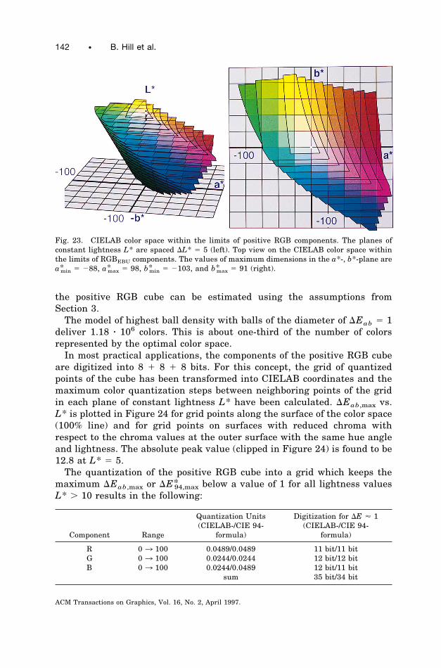
the positive RGB cube can be estimated using the assumptions fromSection 3.

The model of highest ball density with balls of the diameter of DEab 5 1deliver 1.18 z 106 colors. This is about one-third of the number of colorsrepresented by the optimal color space.

In most practical applications, the components of the positive RGB cubeare digitized into 8 1 8 1 8 bits. For this concept, the grid of quantizedpoints of the cube has been transformed into CIELAB coordinates and themaximum color quantization steps between neighboring points of the gridin each plane of constant lightness L* have been calculated. DEab,max vs.L* is plotted in Figure 24 for grid points along the surface of the color space(100% line) and for grid points on surfaces with reduced chroma withrespect to the chroma values at the outer surface with the same hue angleand lightness. The absolute peak value (clipped in Figure 24) is found to be12.8 at L* 5 5.

The quantization of the positive RGB cube into a grid which keeps themaximum DEab,max or DE*94,max below a value of 1 for all lightness valuesL* . 10 results in the following:

Component Range


formula)


formula)

R 0 3 100 0.0489/0.0489 11 bit/11 bitG 0 3 100 0.0244/0.0244 12 bit/12 bitB 0 3 100 0.0244/0.0489 12 bit/11 bit

sum 35 bit/34 bit

Fig. 23. CIELAB color space within the limits of positive RGB components. The planes ofconstant lightness L* are spaced DL* 5 5 (left). Top view on the CIELAB color space withinthe limits of RGBEBU components. The values of maximum dimensions in the a*-, b*-plane area*min 5 288, a*max 5 98, b*min 5 2103, and b*max 5 91 (right).



If the positive RGB cube transformed into CIELAB coordinates as shown inFigure 23 is quantized, the results will be much better and 8 1 8 1 8 bitare sufficient:

Fig. 24. Maximum color difference DEab,max (top) and DE*94,max (bottom) for the digitizationof the positive RGB cube (8 1 8 1 8 bit) along the border in the plane of given lightness. 0%:test points along the grey axis. Other: test points along lines “parallel” to the borderline atreduced chroma given in percent.



Component Range Quantization Units Digitization for DE ' 1

a* 288 3 98 0,7294 8 bitb* 2103 3 91 0,7608 8 bitL* 0 3 100 0,3922 8 bit

sum 24 bit

6.2 Predistorted Positive R9G9B9 Cube (ITU-R BT.709)

As most of the electrical signals for controlling displays use predistortedR9G9B9 components, results for the quantization of a predistorted R9G9B9color space with g 5 2.2 are given in Table VIII. Curves DEab,max versus L*for this case are given in Figure 25. As outlined in Section 4.3, predistortionreduces the color steps due to quantization in the range of low lightness. Itis obvious from Figure 25 that predistortion within the limits of a positiveRGB cube delivers a remarkable improvement of DEab,max compared toFigure 24. This looks even better if the calculation is based on DE*94 (Figure25, bottom). Accordingly, the quantization under the condition of DEab,max# 1 leads to a win of 7 bits compared to the quantization of the positiveRGB cube using undistorted tristimulus RGB components.

Component Range


formula)


formula)

R9 0 3 1 0.00196/0.00196 9 bit/9 bitG9 0 3 1 0.00196/0.00196 9 bit/9 bitB9 0 3 1 0.00098/0.00196 10 bit/9 bit

sum 28 bit/27 bit

For comparison, the YCC color space as described in Section 4.3 anddefined in Kodak [1992] has been analyzed as well for the range of inputcomponents within the positive RGB cube. The maximum color quantiza-tion steps DEab,max vs. L* are shown in Figure 26. Peak color quantizationsteps of up to 5.8 do appear. However, they lie in a range L* , 20 and aremuch smaller than the peak errors in the YCC space limited by optimalcolors. The curves DE*94,max[L*$10] # 1 have a different distribution alongL* in this case, although the amplitudes are nearly the same.

6.3 Color Spaces of Technical Print Processes

6.3.1 Thermal Dye Sublimation Printer. One of the most successfultechnologies in the electronic printing of full color images is that of thethermal dye sublimation printer. The color space of the MitsubishiS3600-30 sublimation printer has been analyzed and the gamut of colorshas been derived by printing a selected number of test colors and determin-ing the respective tristimulus values by accurate spectral measurementequipment. An optimized three-dimensional transformation and interpola-tion algorithm has been developed to determine intermediate color valuesand to describe the surface of the resulting color space. The graphical



presentations in Figure 27 are again composed of the planes of constantlightness L*. The color gamut has been derived for the printer option withonly three printing colors (CMY).

Fig. 25. Maximum color quantization steps DEab,max (top) and DE*94,max (bottom) vs. light-ness L* for the digitization of the predistorted R9G9B9 color space (8 1 8 1 8 bit). 100%: testpoints along the border in the plane of given lightness. 0%: test points along the grey axis.Other: test points along lines “parallel” to the borderline at reduced chroma given in percent.



Fig. 26. Maximum color quantization steps DEab,max (top) and DE*94,max (bottom) vs. light-ness L* for the digitization of the YCC space (8 1 8 1 8 bit) assuming positive RGBcomponents only. 100%: test points along the plane of given lightness. 0%: test points alongthe grey axis. Other: test points along lines “parallel” to the borderline at reduced chromagiven in percent.



For device-independent color description, it is necessary to reference themeasured tristimulus values of a printed test sheet to an absolute stan-dard. Therefore the value of L* 5 0 has been attached to absolutely blackand L* 5 100 to white (barium sulfate white standard) for the illuminantD65. Within this scale, the printer does not reproduce values below L* 5 18and above L* 5 95 with three colorants. The white point of the paper isfound at L* 5 95.

The number of colors resulting from the model of highest ball density is0.627 z 106. In this case, about 50% of the colors of the RGB space areincluded. However, the RGB color space does not surround the color spaceof the sublimation printer completely. In the range of dark colors, there areareas where the colors of the thermal dye sublimation printer lie outsidethe RGB color space.

In Figure 28, the plane L* 5 50 of the color space of a thermal dyesublimation printer has been plotted together with the border lines of theRGB space and the optimal color space.

There is a large area of colors in the range of saturated blue and greencolors that can be reproduced by the thermal dye sublimation printer butnot by the positive components of RGB. On the other hand, a large part ofcolors of the RGB space cannot be reproduced by the printer. If anelectronic image to be printed contains those colors, they must be replacedby other printable colors using gamut mapping.

The quantization is required to describe the full range of reproduciblecolors of the dye sublimation printer in the CIELAB space.

Fig. 27. CIELAB color space of the Mitsubishi S3600-30 thermal dye sublimation printer.The planes of constant lightness L* are spaced DL* 5 5 (left). Top view on the CIELAB colorspace within the limits of CMY printing dye values between 0% and 100%. The values ofmaximum dimensions in the a*-, b*-plane are a*min 5 272, a*max 5 78, b*min 5 258, andb*max 5 95 (right).



Component Range Quantization Units Digitization for DE ' 1

a* 272 3 78 0,5882 8 bitb* 258 3 95 0,6000 8 bitL* 18 3 95 0,6063 7 bit

sum 23 bit

Control of the printer by CIELAB values of 8 1 8 1 7 bits is accordingly themost effective way to represent all the printable colors. If, however, theprinter is controlled by RGB signals, the following quantization wouldbe required under the assumptions of keeping DEab,max[L*$10] # 1 orDE*94,max[L*$10] # 1. No improvement is achieved on the basis of the CIE 94formula in this case.

Component Range


formula)


formula)

R 29 3 103 0,1095/0,1095 10 bit/10 bitG 0 3 104 0,0508/0,0508 11 bit/11 bitB 22 3 112 0,1114/0,1114 10 bit/10 bit

sum 31 bit/31 bit

6.3.2 Cromalin and Match Print Proofing Systems. The Cromalin andMatch Print processes are often used for proofing purposes in professionalprinting. Figure 29 shows both color spaces in CIELAB coordinates.

The number of printable colors estimated from the model of highest balldensity results in 0.484 z 106 for the Cromalin process and in 0.455 z 106 forMatch Print. Hence the number of printable colors is of the same order for

Fig. 28. Plane L* 5 50 of the color space of thermal dye sublimation printer (colored) andborder lines of the positive RGB cube (thin line) and the optimal color space (thick line).



both printers, although there are some differences in detail. More colors arereproduced by the Cromalin process in the blue range, whereas MatchPrint reproduces a few more green colors. It is also obvious that the colorspace of the thermal dye sublimation printer occupies a larger range ofcolors than the conventional proofing systems considered (see Figures 27and 29). This fact is also demonstrated by the planes of constant lightnessL* 5 50 in Figure 30 compared to Figure 28.

Only a small part of the colors of the RGB space is occupied by therespective gamuts of the print process. This points to the difficulty whencomparing images displayed on a cathode ray tube with prints. A goodcorrespondence will only be achieved if the display is controlled via a colorprocessor that reduces the colors of an electronic image to the gamut of theprinter using the same gamut mapping as applied to the print process.

Fig. 29. Cromalin (upper) and Match Print (lower) color spaces given in CIELAB coordinates.



Quantization of the color gamut of the printers requires slightly lesseffort than quantization of the RGB space. The digitization for the twoproofing processes sums up to the same order as that derived for thethermal dye sublimation printer (see Section 6.3.1), that is, 7-bit for thelightness and 8-bit for the a* and b* signals.

Fig. 30. Planes of constant lightness L* 5 50 of the Cromalin (upper) and Match Print(lower). The positive RGB limit is given by thin lines and the border of optimal colors by thicklines, respectively. The assumed light source is D65.



SUMMARY AND DISCUSSION

The CIELAB color space within the limit of optimal colors has beendiscussed and presented in graphical form by plotting planes of constantlightness L* with a net of lines parallel to the a* and b* axes. These planesand the net of a* 2 b* lines has afterwards been transformed into the CIEXYZ, into a standardized tristimulus RGB, a predistorted R9G9B9 space,and the YCC color space of the Photo CD. The planes of constant lightnesswith the net of a* 2 b* lines uniform in the CIELAB space appear distortedafter transformation into the various other color spaces. The distortion andcompression of L*a*b* cells points to the areas of low or high sensitivitywith respect to the color difference perception given in DEab units. Ingeneral, the most sensitive areas are found at the border of optimal colorsin the green to yellow range depending on their lightness. In the CIE XYZspace, the most sensitive areas are located at low lightness, which followsdirectly from the definition of the CIELAB formula. In the tristimulus anddistorted RGB spaces, the dependence on lightness is not that simple andsensitive areas with respect to color difference perception are found at lowand medium lightness. The planes of constant lightness in predistortedcolor spaces are bowed.

To gain more insight into the valuation of color differences with theCIELAB formula, the color spaces considered have been quantized into auniform grid of points and the grid has then been transformed into theCIELAB space, where it has become distorted. Maximum color differencesbetween adjacent points of the grid in CIELAB coordinates have beencalculated as a function of hue angle, lightness, and relative chroma to geta feeling for the distribution and variations of color differences and maxi-mum values when switching color in digital steps. Around each test pointconsidered in a quantized color space, the color differences to neighboringquantized points depend on the direction in the color space and a maximumcolor difference (worst color quantization step) is always found for one ofthe directions of digital steps. If the worst quantization steps along lines oftest points at constant lightness are plotted for the chroma values ofoptimal colors or along chroma values defined by the RGB components of apositive RGB cube, variations of 1:3 to 1:6 are found in all the color spacesconsidered if the CIE 1976 formula DEab is used for the valuation of colordifferences. Still higher variations up to 1:25 are observed for the maxi-mum quantization step within each plane of constant lightness versuslightness L*. The largest color quantization steps are always found at theborder of the color spaces. Much smaller variations appear if the new colordifference formula CIE 1994, DE*94 is used. In this formula, quantizationsteps of chroma are valued much less if chroma values are high.

Predistortion of color spaces based on RGB components reduces the colorquantization steps preferably on the range of low lightness. Peak colorquantization steps in the range of medium lightness are, however, notsufficiently affected by predistortion for the case of the optimal color spaceif the CIE 1976 formula DEab is used. Only for the smaller color spaces on



the basis of RGB components within a positive cube, predistortion resultsin essential advantages. This is demonstrated for the case of the YCC colorspace, where maximum color quantization steps of 16.5 are found for thestandard 8 1 8 1 8 bit quantization concept if colors within a gamut ofoptimal colors or close to an optimal color boundary are considered. Forcolors limited to the positive RGB cube, the maximum quantization steps inthe YCC color space are reduced to the order of 2 to 5. If the CIE 1994formula is used as a basis for color difference calculation, the predistortionresults in essential advantages compared to a linear RGB space.

Suitable quantization concepts for color spaces have been derived in thisarticle from the maximum color quantization step found in each colorspace. The number of required bits per component has been derived on thecondition of keeping the maximum color quantization step just equal to orbelow a value of 1. For the quantization of the CIELAB space itself, theL*a*b* axes have to be digitized into 8 1 9 1 9 bits 5 26 bits. Many morebits are required for the CIE XYZ optimal color space (13 1 13 1 12 bits 538 bits) on the basis of the CIE 1976 color difference formula, the tristimu-lus RGB optimal color space (13 1 12 1 12 bits 5 37 bits), and thepredistorted R9G9B9 optimal color space (12 1 12 1 12 bits 5 36 bits). Forthe limitation of RGB components to the positive cube, 11 1 12 1 12 bits 535 bits are required in tristimulus RGB components and 9 1 9 1 10 bits 528 bits for the predistorted R9G9B9 space. If the positive RGB cube istransformed and quantized in CIELAB coordinates, only 8 1 8 1 8 bits 524 bits are sufficient. Calculation of quantization on the basis of the CIE1994 formula results in less effort in most cases (12 1 12 1 11 bits for thetristimulus RGB optimal color space, 10 1 10 1 9 bits for the predistortedRGB optimal color space, 11 1 12 1 11 bits for the positive RGB cube, and9 1 9 1 9 bits for the predistorted positive RGB cube).

The quantization concepts as derived in this article lead to more conser-vative results than those published in previous work. In Kasson andPlouffe [1992], the quantization error defined as the average statisticalquantization error and the three-sigma error has been calculated for anumber of color spaces assuming quantization into 8 bits per component.For quantization of the CIE XYZ space, the average three-sigma errorresults in 4, for the CIELAB space 0.5 is given, and for the SMPTE-C/2.2color space (predistorted R9G9B9 space with gamma 5 2.2) a value of 2results. Approximately, the reduction of the average error by the factor of 2requires 1 bit more per component. On the basis of this relation, the CIEXYZ space would require 30 bits, the CIELAB space 21 bits, and theSMPTE space 27 bits. For further comparison with the results in thispaper, it has to be considered that a mixture of valuation by the CIELABand CIELUV color difference formula has been used in Kasson and Plouffe[1992] and the gamut of surface colors is a bit smaller than that of optimalcolors. The latter might be the reason for less effort in the quantization ofthe CIELAB space derived in Kasson and Plouffe [1992] (7-bit difference).

The main difference of the results comes from the use of statisticallyaveraged values compared to the use of peak values in this article. As



shown here, peak values of color differences by quantization effects deviatestrongly from average values and hence, even the use of a three-sigmaerror leads to smaller bit numbers. Only for the case of the predistortedR9G9B9 color space, do the results in this article come to the same order asthose published in Kodak [1992] for the SMPTE space (1-bit difference). InStokes et al. [1992a], the necessary quantization of a predistorted R9G9B9space for the control of cathode ray tubes has been estimated by 7.4 bits percomponent or 22 bits in total, also assuming a threshold limit of the orderof 1. This comes close to the results of 23 bits derived in this article. Again,the published result is based on the statistical averaging of quantizationeffects, but the variation of color quantization steps for the positive R9G9B9space (see Figure 25) has been found to be comparatively small.

The question of whether a quantization concept should be based onaveraged values or peak values cannot be answered generally. It wouldhelp to investigate experimental data on the perceptible thresholds of thespecific colors in the sensitive areas of a color space, where peak colorquantization steps appear.

The studies on quantization effects have also been applied to a number ofprint processes (thermal dye sublimation, Chromalin, and Match Print).The device-dependent color spaces of these processes have been developedfrom measured data and plotted in L*a*b* coordinates. Due to their smallcolor gamut, the quantization into 7 1 8 1 8 bits is sufficient to keep themaximum color quantization steps below 1. If the same gamut of colors isrepresented in tristimulus RGB components, 31 bits are required for thesame precision, if DEab is considered.

With the assumption of a just-noticeable threshold of color perception ofDEab 5 1, a rough estimation of the number of distinguishable colorsincluded in the optimal color space results in 3.2 z 106. The same kind ofestimation results in 1.1 z 106 just-noticeable colors included in a positiveRGB cube, and the order of 0.45 to 0.48 z 106 is found for the color spaces oftechnical print processes, respectively. Hence, practical prints resolve onlyabout 1/7 of the whole number of surface colors.

The comparison between the CIELUV and the CIELAB space by valuat-ing the color differences in the CIELUV space by the CIELAB colordifference demonstrates a strong inconsistency between both color differ-ence definitions, particularly in the range of blue and green colors. If colordifferences are calculated with the CIE 1994 formula, a good match to theworst case color differences of the CIELUV space is found for all colors ofhigh lightness. Only in the range of low lightness, strong differences stillappear. The new color difference formula CIE 1994 is considered todescribe color difference perception more consistent with experimentalresults. All the curves describing the distribution of color difference stepsoutlined in this article appear more uniform on the basis of this formulaand result in lower numerical values in most cases. This is certainly anadvantage for practical applications, even if the difficulty now is that therepresentation of colors in the established CIELAB space is not moreconsistent with uniform color difference valuation.



REFERENCES

ALMAN, D. H. 1993. CIE Technical Committee 1-29. Industrial color difference evaluation.Progress report. Color Res. Appl. 18, 137–139.

CCIR. 1982. CCIR Recommendation 601-1. Encoding parameters of digital television forstudios. Geneva 1982–1986.

CCIR. 1990. CCIR Recommendation 709 (1990). Basic parameter values for the HDTVstandard for studio and for international programme exchange. Geneva.

CIE. 1986a. Colorimetry. CIE Pub. 15.2, 2nd ed., Commission International de L’Eclairage,Vienna, 29–30.

CIE. 1986b. Colorimetry. CIE Pub. 15.2, 2nd ed., Commission International de L’Eclairage,Vienna, 30–31.

CIE. 1986c. Colorimetry. CIE Pub. 15.2, 2nd ed., Commission International de L’Eclairage,Vienna, 56–58.

CIE. 1993. Parametric effects in color-difference evaluation. CIE Pub. 101, CommissionInternational de L’Eclairage, Vienna.

CIE. 1995. Industrial color-difference evaluation. CIE Pub. 116, Commission Internationalde L’Eclairage, Vienna.

KASSON, M. J. AND PLOUFFE, W. 1992. An Analysis of Selected Computer Interchange ColorSpaces. ACM Trans. Graph. 11, 4 (Oct.), 373–405.

KODAK. 1992. Photo CD products 1992. A planning guide for developers. Kodak PartNumber DCI-200RJ Rochester, NY.

LANG, H. 1978. Farbmetrik und Farbfernsehen. Oldenbourg, Munich.LANG, H. 1995. Farbwiedergabe in den Medien, Fernsehen, Film, Druck. Muster-Schmidt

Verlag, Gottingen, Zurich.LOO, M. R. AND RIGG, B. 1987. BFD (l:c) colour-difference formula. Part 1: Development of

the formula. JSDC 103 (Feb.), 126–132. Part 2: Performance of the formula. JSDC 103(March), 86–94.

MACADAM, D. L. 1935a. The theory of the maximum visual efficiency of color materials. J.Opt. Soc. Am. 25, 249.

MACADAM, D. L. 1935b. Maximum visual efficiency of color materials, J. Opt. Soc. Am. 25,361.

MAHY, M., MELLAERT, B. V., AND VAN EYCKEN, O. A. 1991. The influence of uniform colorspaces on color image processing: A comparative study of CIELAB, CIELUV, and ATD. J.Imag. Technol. 17, 5 (Oct.), 232–243.

POINTER, M. R. 1980. The gamut of real surface colours. Color Res. Appl. 5, No. 3, 145–155.RICHTER, M. 1979. Einfuhrung in die Farbmetrik. 2. Auflage 1981, de Gruyter, New York.ROSCH, S. 1929. Darstellung der Farbenlehre fur die Zwecke der Mineralogie, Fortschr.

Mineral. Krist. Petrogr. 13, 143.SAE. 1985. SAE J 1545 1985. Recommended practice, instrumental color difference mea-

surement for exterior finishes, textiles, and colored trim. SAE.SCHRODINGER, E. 1920. Theorie der Pigmente von großter Leuchtkraft, Ann. Physik (IV) 62,

603.SCHWARZ, M. W., COWAN, W. B., AND BEATTY, J. C. 1987. An experimental comparison of

RGB, YIQ, LAB, HSV, and opponent color models. ACM Trans. Graph. 6, 2 (April), 123–158.STOKES, M., FAIRCHILD, M. D., AND BERNS, R. S. 1992a. Precision requirements for digital

color reproduction. ACM Trans. Graph. 11, 4 (Oct.), 406–422.STOKES, M., FAIRCHILD, M. D., AND BERNS, R. S. 1992b. Colorimetrical quantified visual

tolerances for pictorial images. In Techn. Association of the Graphic Arts, TAGA Proceed-ings, vol. 2, M. Pearson Ed., 357–777.

Received June 1994; revised November 1996; accepted January 1997



Documents

Comparative Analysis of the Quantization of Color Spaces on the