COMPARATIVE ANALYSIS OF THE HEDGING EFFECTIVENESS …

Revista de Economia, v. 37, n. 3 (ano 35), p. 21-46, set./dez. 2011. Editora UFPR70

COMPARATIVE ANALYSIS OF THE HEDGING EFFECTIVENESS FOR SOYBEAN USING OLS AND

BIVARIATE GARCH BEKK MODEL

Carlos Eduardo Caldarelli1

Waldemar Antônio da Rocha de Souza2

Abstract: Dynamic hedging effectiveness for soybean farmers in Rondonópolis (MT) with futures contracts of BM&F-BOVESPA is calculated through optimal hedge determination, using the bivariate GARCH BEKK model, which considers the con-ditional correlations of the prices series, comparing the results with the minimum variance model effectiveness, calculated by OLS, the unhedged and the naïve hedge positions. The financial effectiveness of the dynamic hedge model is superior and can be used by farmers for several decision making purposes such as price discovery, hedging calibration, cash flow projections, market timing, among others.

Keywords: Dynamic hedge; minimum variance; soybeans; Mato Grosso.

Resumo: As taxas ótimas de hedge para os produtores de soja em Rondonópolis (MT), através de contratos futuros da BM&F-BOVESPA, são comparadas através das duas principais abordagens para a determinação de hedge ótimo, o modelo de mínima variância, por MQO, e o modelo GARCH BEKK bivariado, o qual considera as correlações condicionais das séries. A efetividade financeira do modelo de hedge dinâmico apresenta-se superior, e pode ser usada pelos produtores para uma série de tomada de decisões tais como descoberta de preços, ajuste de taxa de hedge, projeções de fluxo de caixa, no processo de market timing entre outras.

Palavras-chave: Hedge dinâmico; mínima variância; soja; Mato Grosso.

1 Professor Adjunto da Universidade Federal da Grande Dourados – UFGD.2 Professor Adjunto da Universidade Federal do Amazonas – UFAM

Revista de Economia, v. 37, n. 3 (ano 35), p. 70-91, set./dez. 2011. Editora UFPR 71

CALDARELLI, C. E; SOUZA, W. A. R. Comparative analysis of the heading effectiveness ...

Introduction

In the last three decades Brazilian agribusiness has played a pivotal role in foreign exchange generation and regional economic development, particularly in the Centralwestern Region. With the continuous growth in size, competi-tiveness and complexity of the agricultural sector in the last few years, infor-mation has become a strategic input for decision making in the production.

Within this framework, the soybean supply chain became particularly relevant to the Brazilian agribusiness. In the last ten years, the harvested area of the grain has grown at an annual average rate of 8,1%, boosted by an expanding foreign demand, turning the country into a major supplier of the commodity worldwide (MAPA, 2007).Soybean cultivation was introduced in Brazil be-fore the 50´s and in the 70 and 80´s a rapid growth happened, stabilizing through the 80´s. In the 90´s and 2000 there was a large increase in the crop production, turning the country the second producer worldwide (SANCHES; MICHELLON; ROESSING, 2004).

There are price and volatility risks associated with the soybean production, both with a negative impact over that industry revenues. One possibility for offsetting the price risk is through the usage of futures contracts, which have been, however, underutilized by Brazilian farmers (MARQUES; MELLO; MARTINES-FILHO, 2008).

The research question addressed in this article is the measurement of the hedging effectiveness of the dynamic hedge ratios, evaluating its performance vis-à-vis other hedging strategies, for the soybean farmers in Rondonópolis (MT), using futures contracts of BM&F-BOVESPA3. The results have many applications in the supply chain of the crop, particularly in the price disco-very process, hedging ratio calibration, cash flow projections, undertaking of financial leverage and marketing decisions, as well as in the expansion of futures contracts usage in the local futures exchange.

The survey questions are: i.) how to calculate the hedging ratios in the bivariate GARCH BEKK (dynamic hedge) and the minimum variance (OLS) models; ii.) what is the hedging effectiveness of the dynamic hedge compared with the unhedged, the “naïve” and traditional model, by OLS, portfolio positions ; and, iii.) what are the intrinsic properties of the dynamic hedging ratios time series, such as the existence of unit root.

The results contribute to the academic research in futures markets, using a state-of-the-art model to obtain the dynamic hedge ratios for Brazil´s most traded agricultural commodity, applied to the largest producer region in the domestic futures market.

3 BM&F-BOVESPA is the Brazilian equity and futures exchange, a new corporation which resulted from the merger between BOVESPA and BM&F, both of which were previously independent companies.

72 Revista de Economia, v. 37, n. 3 (ano 35), p. 70-91, set./dez. 2011. Editora UFPR


The article is divided as follows: section 2 reviews the literature, section 3 describes the OLS, the GARCH BEKK and other hedging methodologies, the parametric tests and the data set, section 4 presents and discusses the results and section 5 concludes the study.

1. Literature review

Most of the current literature about hedging strategies studies the optimal hedge ratios, i.e., the ratio between spot and futures markets position which minimizes an individual agent’s price risk using futures contracts.

Hedge is defined in the literature as the strategy of agents willing to transfer risk among themselves, primarily hedgers and speculators. When a hedger offsets its price risk, he becomes exposed to basis risk, which is the instability between spot (in the price reference market) and futures prices (LEUTHOLD ET AL., 1989).

Marques et al. (2008) described hedging in the futures market as the agent holding contrary spot and futures markets positions, taking the futures con-tracts settlement date as reference for trading.

Collins (1997) indicated that most of the hedging literature focuses on how the market players can use the futures market to offset their risks, therefore optimizing their price, output, income and profit objectives. As such, several hedging strategy models have been studied throughout time, which fundamen-tally converge to decision models for the hedging effectiveness, considering most influencing factors as close as possible to the agent realities.

The risk offsetting proportion, i.e., the ratio of the agent´s position, the number of contracts to be traded, in the futures market relative to his spot market position defines the hedge ratio, which is an outstanding reference in the literature. Carter (1999) showed that most of the literature concerning hedge in the past fifty years investigates the optimal hedge ratio.

Some models study the expected utility in hedging, such as Johnson (1960), Stein (1961) and Grant (1989), using the minimum variance framework to obtain the optimal hedge ratio. Others include some degree of flexibility, as in Lence (1996), to proxy the decision making process of the agents. All this research effort focuses the optimal hedge ratios.

Considering the agent´s decision making process, one of his goals is the risk minimization of his overall position in the commodity market, as in a optimal portfolio evaluation. Therefore, the optimal hedge ratio can be different of the unity, since part of the output is traded in the futures market and the



balance in the cash market. Finding this optimal hedge ratio, the minimum variance hedge, is the fundamental goal when one trades in the futures ma-rkets (HULL, 2003).

Figure 1 shows the optimal hedge position, or minimum variance, in a risk and return framework.

FiGUre 1 – risk, reTUrn AnD OPTiMAl HeDGe rATiO

SOURCE: Authors, based in Leuthold et. al. (1989).

As shown in Figure 1, the optimal hedge ratio is the quotient between the futures and the spot markets position that minimize the portfolio risk in the efficient frontier, i.e., the position that maximizes return and minimizes the expected return variance. Henceforth, this optimal hedge ratio is equivalent to the minimum variance hedge ratio, which does not consider any agent’s utility and preference issues.

There are studies in Brazil approaching the optimal hedge, such as Silva et al. (2003), who evaluated the hedging effectiveness of soybean oil, meal and grain in CBOT and BM&F, finding that a cross-hedging strategy with grain futures in BM&F has a low degree of effectiveness for the oil and meal, while the equivalent contracts in CBOT showed better results.

Santos et al. (2008) investigated the minimum variance hedge in BM&F for the Centralwestern soybean production, between October of 2002 and December of 2005, concluding that 44% of the output of the Goiás soybean could be hedged with futures contracts to offset 35% of its price risk.

Martins and Aguiar (2004) studied the futures contracts timeframes in CBOT to discover those with higher degree of hedging effectiveness for the Brazilian soybean output cycle, concluding that the contracts settled in the second half



of the year, in particular the months of July and August, were the most effec-tive. Also found a higher effectiveness in the regions closer to the exporting ports of São Paulo and Paraná.

The Brazilian studies approached the optimal hedge strategy following a particular methodology. As such, a necessary consequent step is to compare the two main methodological hedging frameworks, the minimum variance and the generalized autoregressive conditional heteroskedasticity (GARCH) models, applied to a sample region of soybean market in Brazil, which is the contribution of the present article.

2. Methodology and data

Two methodologies were considered for the optimal hedge ratios of the soybean farmers in Rondonópolis (MT) through futures contracts in BM&F-BOVesPA, within a time period. The first method was ordinary least squares (OLS), based in the constant covariances matrix hypothesis. The second was the GARCH BEKK model, which considers the time dependence of the covariances matrix, yielding a dynamic hedge ratio for each time period considered.

The hedging effectiveness was calculated for both the minimum variance and the dynamic hedge ratios, on a portfolio optimization framework, comparing with an unhedged and a “naïve” hedge positions. Also, the existence of unit root, as well as cointegration, was tested for the price levels for time series analytical purposes, as this is a usual procedure for the analysis of dynamic hedges (BROOKS ET AL., 2002).

2.1. Minimum Variance Hedge Model

For Hull (2003) the optimal hedge ratio describes the futures and spot ma-rkets position of an agent that minimizes price variance if he is a risk averter. This ratio is given by:

)(),(

t

tt

FVarFSCOV

∆∆∆ Eq. (1)



where:

=∆ tS spot prices first difference;=∆ tF futures prices first difference.

Leuthold et al. (1989) showed that these variables are calculated through the ordinary least squares (OLS) estimation of:

tt FS ∆+=∆ ba Eq. (2)

where:

=ba , are linear parameters of the model;

In Equation 2 the estimated β indicates the total output ratio that should be traded in the futures markets yielding the least variance, the minimum va-riance optimal hedge ratio. The standard coefficient of determination – 2R – in the Ols models, indicates the hedging effectiveness, the decrease in the price variance of the agent´s total position, given by the sum of his spot and futures markets positions (HULL, 2003).

However, the minimum variance optimal hedge methodology must be eva-luated with limits, as there are evidences, such as serial correlation and he-teroskedasticity, that results are dependent of the commodity price variation conditional distributions, which will change in time when the conditional distribution varies, with a high degree of probability.

in this regard, the White´s heteroskedasticity and the ljung-Box serial corre-lation tests were calculated, to analyze if the covariances matrix conditional distribution is non-constant and the GARCH BEKK model can be applied to calculate conditional variation adjusted hedge ratios.

2.2. Multivariate GARCH Models

The minimum variance hedge is widely used and can be easily estimated. However, empirical approaches have shown that the variances of most pri-ce series are not constant over time, with volatility clustering, particularly financial and agricultural price series. Therefore, any realistic hedge ratio estimation for agricultural prices should consider this property.

To address this situation, multivariate Generalized Autoregressive Conditio-nal Heteroskedastidity (GARCH) models were adopted in several empirical



studies: Ballie and Myers (1991), Myers (1991), Haigh and Holt (2000, 2002), Yang (2000).

According to Hamilton (1994), an Autoregressive Conditional Heteroskedas-tidity –ArCH(m) process (u

t), is described by:

ttt vhu .= Eq. (3)where v

t is an i.i.d. sequence with zero mean and unit variance and h

t evolves

according to:

2222

211 ... mtmttt uuuh −−− ++++= aaaz Eq. (4)

In general terms, there could be a process for which the conditional variance depends on an infinite number of lags of 2

jtu − ,

2)( tt uLh pz += Eq. (5)

where ∑∞

=

=1

)(j

jjLL pp

A natural approach is to parameterize )(Lp as the ratio of two finite-order polynomials:

,...1

...)(1

)()( 22

11

22

11

rr

mm

LLLLLL

LLL

dddaaa

da

p−−−−

+++=

−= Eq. (6)

where the roots of 0)(1 =− Ld are outside the unit circle. If Equation 5 is multiplied by )(1 Ld− , the result is

[ ] [ ] 2)()1(1)(1 tt uLhL azdd +−=−

or

2222

211

2211

...

...

mtmtt

rtrttt

uuuhhhh

−−−

−−−

++++

++++=

aaa

dddk Eq. (7)

for [ ]zdddk r−−−−≡ ...1 21

Equation 7 is the ut ~ GARCH(r, m) model, as proposed by Bollerslev (1986),

where ht is the forecast of 2

tu based on its own lagged values and ttt huw −= 2

is the error associated with this forecast, wt is a white noise process. Therefore,

if ut is a GARCH(r,m) process, then 2

tu follows an ARMA (p,r), p = maxr,m. The nonnegativity requirement is satisfied if κ>0 and 0,0 ≥≥ jj da , for j =



1, 2, …, p and 2tu is covariance stationary. The forecast of 2

stu + based on past values can be calculated by iteration.

Calculation of the sequence of conditional variances Ttth 1= from Equation 7 requires presample values for 0,...,1 hph +− and 2

0,...,21 upu +−

. If there are ob-servations on y

t and x

t for t = 1, 2, …, T, Bollerslev (1986) suggested setting:

2^2 s== jj uh for j=-p+1,…,0,

where ( )

2

1

12ˆ ∑=

− ′−=T

ttyT x ts

The sequence Ttth 1= can be used to evaluate the log likelihood function ma-ximimizing numerically with respect to B and the parameters of the GARCH process.

The preceding model can be extended to an ( n x 1 ) vector yt, which comprises

a multivariate GARCH model. Consider a system of n regression equations :

)1()1()()1( ××××+•′=

nt

ktknn

t uxy

where xt is a vector of explanatory variables and u

t is a vector of white noise

residuals. Let Ht denote the (n x n) conditional variance-covariance matrix

of the residuals:

( ),...,,...,,| 121 −−−′= ttttttt E xxyyuuH

A vector generalization of a GArCH(r,m) specification can be:

mmtmtm22t2t211t1t1rrtr22t211t1 Auu...AAuuAAuuAH...HHH ′′+′′+′′+′++′+′+= −−−−−−−−−t

where κ, ∆s and A

s for s = 1, 2, … denote ( n x m ) matrices of parameters, H

t

is guaranteed to be positive definite as long as κ is positive definite, which can be ensured numerically by parameterizing κ as PP’, where P is a lower triangular matrix.

In practice, for reasonably sized n it is necessary to restrict the specification



for Ht further to obtain a numerically tractable formulation. One useful

special case restricts ∆s and A

s to be diagonal matrices for s = 1, 2, … and the

conditional covariance between uit and u

jt depends only on past values of

ui,t-x

.uj,t-s

, and not on the products or squares of other residuals.

There are several approaches for the multivariate GARCH models, such as constant conditional correlations over time among the elements of u

t, the

VECH (Ht), the factor ArCH and the Bekk specifications.

2.2.1. The GARCH BEKK Model

The multivariate GARCH BEKK (q,p,k) model, with the conditional covarian-ces matrix H

t, given the informational set available in t, model, as described

in Baba et al. (1990) and Bittencourt et al. (2006), can be summarized as:

,21

ttt H ne = Eq. (8)

∑∑=

−−−=

′+′′+′=p

jjjtjiitt

q

iit BHBAACCH

11

1ee Eq. (9)

where C, A, B are (k x k) parameters matrices, with k=2, in the bivariate case, C is an upper triangular matrix, p and q are the model orders and k is the number of series used.

The multivariate GARCH BEKK model is covariance stationary if the eigen-values of ( ) ( )′⊗+′⊗∑ ∑= =

q

i

p

j jjii BBAA1 1

are less than one in absolute value, where ⊗ is the Kroneker product.

As Karolyi (1995) ilustrated, the BEKK model has a particularity in its speci-fication: the generalized configurations, allowing cross impacts between the conditional variances and covariances of the variables, while not demanding a large number of parameter estimations. The model is estimated through the Quasi-maximum Likelihood Method, adopting the a Gaussian assump-tion for the errors. Jeantheau (1998) demonstrated the strong consistency of quasi-maximum likelihood estimators in multivariate GARCH models, even if the data is approximately non-normal, thus justifying its features and framework.

In the GARCH BEKK model, the dynamic (optimal) hedge ratio can be obtained, when the return is equal to the log differences of the commodity prices, as:



)|()|,( 1111 −−−− Ω∆Ω∆∆= tttttt fVarfpCovb Eq. (10)

Where 1−tb indicates the dynamic (optimal) hedge ratio, tp and tf are the logs

of spot and futures prices respectively, given the time 1−t and the informa-tion set – 1−Ωt .

Baillie and Myers (1998) and Benninga et al. (1984) showed that variance minimization implies a high degree of risk aversion. However, if the expected return of the hedge is zero, then the minimum variance hedge rule will be the maximum expected hedge utility rule, generalizing the use of the minimum variance approach.

To calculate the dynamic hedge ratios, given the spot and futures prices wi-thin a period of time, a GArCH Bekk bivariate model, specified in equation 10, is used. An optimal hedge ratio vector b

t-1 can be obtained through the

conditional covariance matrix Ht, as:

t

tt h

hb,22

,211 =− Eq. (11)

where tijh , is the i-eth row and j-eth column element of the conditional cova-riance matrix H

t. The optimal dynamic hedge ratio, in sampled estimates,

can be obtained with Ht, and its matrix representation is:

′

+

′

+

=

−−

−−

−−−

−−−

2221

1211

1,221,21

1,121,11

2221

1211

2221

12112

1,21,11,2

1,21,12

1,1

2221

1211

22

2111

2221

11

,22,21

,12,11

00

bbbb

hhhh

bbbb

aaaa

aaaa

ccc

ccc

hhhh

tt

tt

ttt

ttt

tt

tt

eeeeee

2.3. Hedging Effectiveness

For the minimum variance and dynamic hedge ratios, calculated through the OLS and GARCH BEKK models respectively, the hedging effectiveness will be derived from the time varying and constant portfolios using the output of



the models, as in Brooks et al. (2002).

For the dynamic hedge ratios portfolio, at time t-1 the expected return )(1 tt RE − , of the portfolio comprising one unit of commodity and b units of the futures contract may be written as:

)()()( 1111 ttttttt FESERE ∆−∆= −−−− b Eq. (12)

Where 1−tb is the hedge ratio determined at time t-1, for use in period t. The variance of the expected return ( tp,s ) of the portfolio is:

tSFttFttstp ,1,2

1,, 2 sbsbss −− −+= Eq. (13)where:

tp,s = the conditional variance of the portfolio;

ts,s = the conditional variance of the portfolio spot position;

tF ,s = the conditional variance of the portfolio futures position;

tSF ,s = the conditional covariance between the spot and futures position; and

1−tb = the optimal hedge ratio.

For hedging effectiveness comparison, four different commodity portfolios were dimensioned. First, the unhedged portfolio, where there is only a long position in the commodity spot market.

Second, the “naïve” hedged, taking one short futures contract for every spot market unit, making b equals minus one, but not allowing the hedge to time-vary. The “naïve” hedge proxy the basis risk only portfolio.

Basis is defined as the difference between spot and futures prices, as follo-ws:



ttt FSB −= Eq. (14)

where tB = basis, tS = spot price and tF = futures price.

Therefore:

)()()( 111 tttttt FESEBE ∆+∆=∆ −−− Eq. (15)

Which is equivalent to Equation 14, with t∆Β = tR∆ and 1−=b .

In the third portfolio, the minimum variance hedge, there are the spot and the optimal OLS time invariant hedge ratio positions. And last, the dynamic hedged portfolio, where the spot and dynamic time variant positions are input, using the dynamic (optimal) hedge ratios of the GARCH BEKK model.

The return and variance were calculated for all four portfolios in order to infer which yields the highest degree of effectiveness, measured by the variance reduction vis-á-vis the expected return.

Descriptive statistics evaluation, Augmented Dickey-Fuller (ADF) unit roots and Engle-Granger cointegration tests were performed in both spot and futures price series levels. The ADF unit root test was also performed on the dynamic hedge ratios, given by the GARCH-BEKK model, to verify its weak stationarity property, making possible its ex-ante previsions through the use of ARMA modeling.

2.4. Data

Three sets of data were used. The first one was the spot market soybean daily prices in Rondonopolis (MT), source: ESALQ/CEPEA. The prices are quoted in R$/60 kg bags and were transformed in US dollars to compare with the futures prices of BM&F-BOVESPA contracts quotes. The second was the fu-tures prices series of the soybean contract traded in BM&F-BOVESPA, which has the following specifications:



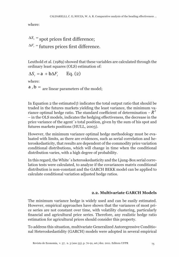
TABle 1 – BM&F-BOVesPA sOyBeAn FUTUres COnTrACTs MAin sPeCi-FICATIONS

ITEM SPECIFICATIONCommodity Brazilian soybean, export type, graded through MAPA

specificationsQuote Usdollars for 60 kgs bagTrade Unit 27 metric tons or 450 bags of 60 kgs Settlement Months March, april, may, june, july, august, september and

novemberSettlement and Last Trading Date

9th business day before the first day of settlement month

Point of delivery and price reference

Paranaguá (PR)

Daily Settlement Based in the settlement price as per the Exchange´s rules

SOURCE: BM&F-BOVESPA (2009)

Carchano and Pardo (2009) showed that among five different methodologies to construct index futures contracts continuous series, for trading as well as academic research purposes, there are not significant differences between the resultant series, indicating that the least complex method can be applied.

In order to obtain a continuous soybean futures price series for the BM&F-BOVESPA contract, the settlement month and its last trading date were con-sidered to construct successive non-overlapping time intervals. The rollover date, the point of time when contract series are switched to the next one, is the 9th business day before the first day of the contract settlement month, as defined in the contract specifications in Table 1.

For example, the last day for the April contract will be the 9th business day before April 1st, when a new interval will be initiated with the prices for the May contract. Therefore, March will have both price series for the April and May contracts, with rollover on the 9th business day before April 1st. For a single year, the continuous futures prices time series intervals were constructed as follows (Table 2).



TABle 2 –sOyBeAn FUTUres COnTrACTs COnTinUOUs PriCe series

MONTH FUTURES CONTRACTS MONTHS*January MarchFebruary March / AprilMarch April / MayApril May / JuneMay June / JulyJune July / AugustJuly August / SeptemberAugust September / NovemberSeptember NovemberOctober November / MarchNovember MarchDecember March

Note: The reference day for the price series rollover date is the 9th business day before the contract month first day.

sOUrCe: Authors, with BM&F-BOVesPA soybean contract specifications.

The third was the Reais/US dollars daily exchange rate series, given by the PTAX-800 selling quotes, of Banco Central do Brasil, used to convert the spot prices, quoted in Reais, in Rondonópolis (MT) to US dollars, in order to compare with the futures contracts in BM&F-BOVESPA.

Estimation period was March 03rd, 2004 up to June 16th, 2009, totaling 1.321 observations of daily quotes. When there was a discrepancy of dates, i.e., local holidays, the price in date t was linearly interpolated between the previous and the next values. The return was calculated by the logarithm difference between two successive values, for both spot and futures series.

The software used was E-VIEWS, version 6, which holds the GARCH BEKK model built-in features.

3. Discussion and results

The daily spot, in Rondonópolis (MT), and futures prices series, in BM&F-BOVESPA, are shown in Figure 2, both series at their levels.



FiGUre 2 – sOyBeAn DAily PriCes sPOT MArkeT in rOnDOnóPOlis (MT), FUTUres in BM&F-BOVesPA (UsDOllArs/60 kG BAG) – DATes: MAr.01/04 TO JUN.16/09

SOURCE: BM&F-BOVESPA (2009)

The first step was the estimation of the minimum variance hedge position using OLS, as shown in Table 3.

TABle 3 – MiniMUM VAriAnCe HeDGe Ols reGressiOn PArAMeTers

Variable Coefficient Standard-Error “t” statistics ProbabilityC 0.018 0.049 0.363 0.717∆Ft 0.499 0.029 17.445 0.000R2 0.188

Note: b = minimum variance hedge is the ∆ft coefficient and r2 its effectiveness.

SOURCE: authors

The minimum variance hedge, b , equals the tF∆ regression coefficient, reaching 0.499, which is the optimal percentage in soybean futures contracts in BM&F-BOVESPA necessary to offset the price risk of the spot position. The minimum variance hedge effectiveness is given by the 2R statistics, 0.188, a low parameter.

The diagnostic tests for the minimum variance hedge model (White´s and ljung-Box), to detect volatility clustering and heteroskedasticity, peculiar of financial and commodity price series, are listed as follows (Table 4).



TABle 4 – DiAGnOsTiC TesTs FOr THe MiniMUM VAriAnCe (Ols) HeDGe MODEL

TEST Test Sta-tistics P-ValueAutocorrelation: Ljung-Box

∆Ft

Q(05) 4.584 0.469 *Q(10) 9.671 0.470 *Q(15) 13.786 0.542 *

∆St

Q(05) 2.417 0.789 *Q(10) 6.880 0.737 *Q(15) 8.811 0.887 *

Heteroskedasticity : White´s 73.539 ** ARCH LM

F-statistics Observed R2

Valor Prob.F, χ2

224.816 0.000***192.327 0.000***

note: (*) rejects the null hypothesis of autocorrelation at the 5, 10 and 15 % significance levels; (**) no rejects the null hypothesis of homoskedasticity at the 5, 10 and 15% significance levels; (***) there is strong evidence of ARCH effects in the residuals.

SOURCE: authors

The ljung-Box test results allow the rejection of the null hypothesis of non-autocorrelation in the residual of the OLS model. However, the White´s test no rejects the null hypothesis of the existence of heteroskedasticity. The results indicate an inappropriate hedge ratio, given by OLS. In the presence of auto-correlation and heteroskedasticity, OLS estimators are undesirable, because are inefficient and the inference based on least squares estimates is adversely affected. However, the ARCH LM results indicate a strong ARCH effect in the OLS residuals. Therefore, the best approach is to use a model considering this feature, such as the GArCH Bekk bivariate model – dynamic model.

The results for the GARCH BEKK bivariate model are shown in Table 5.



TABle 5 – GArCH Bekk BiVAriATe MODel PArAMeTer esTiMATiOnParameters Estimation Standard-Error

C(1) 0.067 0.049C(2) 0.027 0.039

M(1,1) 0.199 0.046M(1,2) 0.077 0.015M(2,2) 0.237 0.040A1(1,1) 0.253 0.017A1(2,2) 0.328 0.013B1(1,1) 0.938 0.009B1(2,2) 0.898 0.012

note: Covariance specification:

BEKK; )1(*11*)1(*1 −+−+= GARCHBARESIDAMGARCH ; M is an indefinite matrix, A1, B1 are diagonal matrices.

SOURCE: authors

in Table 5, the C(1) and C(2) parameters are the spot and futures price coeffi-cients, A

i is the ARCH term matrix, B

j is the GARCH matrix. The parameters of

Ai e B

j are used for volatility transmission. In Figure 3 the minimum variance

and the dynamic hedge ratios, calculated through the OLS and GARCK BEKK models, respectively, are shown.

FiGUre 3 – MiniMUM VAriAnCe AnD DynAMiC HeDGe rATiOs sOyBeAn SPOT AND FUTURES PRICES OUTPUT: OLS AND GARCH BEKK BIVARIATE MODEL

SOURCE authors

For hedging effectiveness comparison, four portfolios were constructed, with an unhedged position, a “naïve”, the minimum variance and dynamic hedges (Table 6).



TABle 6 – HeDGinG eFFeCTiVeness sUMMAry sTATisTiCs FOr POrTFOliO RETURN AND VARIANCE (IN % CHANGE) OF DAILY QUOTES

Parameters Unhedged Naïve M i n Va r i a n c e Hedge

Dynamic Hedge

β 0 -1 0.499 Time varyingReturn 0.034 0.002 0.018 0.033

Variance 3.831 3.837 3.112 3.127

Relativization Naïve M i n Va r i a n c e Hedge

Dynamic Hedge

Return 94.1% -47.1% -2.9%Variance 0.2% -18.8% -18.4%

SOURCE: authors

The unhedged portfolio corresponds to a single long position in the spot market. The return and variance show the Rondonópolis (MT) soybean pri-ce series performance. All the other portfolios return and variance relative performances are compared with the unhedged.

By Table 6, the “naïve” hedge portfolio, holding a long spot and a short futures markets position simultaneously, decreases the return but does not affect the variance. This behavior proxies pure basis risk speculation, i.e., the expected return is neutral and variance depends only on the basis itself.

Composed of a long spot and a short futures markets position, the later equals the spot position multiplied byb , the minimum variance hedge portfolio, decreasing both the return and variance. The variance reduction equals the daily basis price risk neutralization and is larger than the “naïve” portfolio variance decrease.

The dynamic hedge portfolio, which has a long spot market position and a b-time varying futures market short position, does not alter significantly the return of the unhedged portfolio, but has quite the same impact on variance reduction as the minimum variance, as shown in Table 6.

This means that the dynamic hedge portfolio holds the largest hedging effec-tiveness, outperforming all the others, both in terms of constant expected return and price risk minimization, measured by variance reduction. Ano-ther relevant feature of the dynamic hedge portfolio is the stationarity ofb, which can be used for forecasting of the hedging ration through an ARMA approach. Also, as it is time varying, the associated financial costs are less than the other hedges.



4. Summary and conclusions

Deduction of the optimal hedging positions is key to an efficient resource allocation by the hedging agents. The optimal hedge considers the price risk offset and the expected return from the simultaneous spot and futures ma-rkets positions, considering the dynamic behavior of spot and futures prices variances and covariances. The hedger objective is a combination of assets positions in a portfolio comprising of commitments in the commodity spot and futures markets that minimize the portfolio risk within the efficient frontier region. The main function of the futures markets is to provide a financial tool capable of delivering the portfolio optimal combination in a dynamic adjustable setting.

The hedging strategies analyzed encompassed several alternatives, ranging from the simple unhedged, long only, to the dynamic, time varying, positions. Each alternative impacts the risk, measured by the variance, and expected return differently. The hedger continuous efforts are geared toward finding which portfolio combination of spot and futures markets positions better suits his needs and risk perception. Particularly, for the soybean farmers of Rondonópolis (MT), bearing high basis risk, this effort is compensated by the optimal hedging results.

Compared with the unhedged, “naïve” and minimum variance hedges, the dynamic hedge is the most effective to minimize price risk and optimize ex-pected return for the Rondonópolis (MT) soybean production. This result is in line with other studies of dynamic hedge ratios for other commodities and is widely approached for academic research, as well as industry management.

There are several economic and financial impacts of the dynamic hedge stra-tegy on the Rondonópolis (MT) soybean farmers using the BM&F-BOVESPA futures contracts, which will positively affect their decision making process, such as price discovery, hedging calibration, cash flow projections, market timing, among others.

A dynamic, time varying, hedge, considering the intrinsic characteristics of the price series volatility, has a major contribution in offsetting the rondonópolis (MT) soybean price risk, which is a seasonal, storable commodity, affected by a high basis risk. That will contribute for a better resources allocation by the industry, increasing the returns throughout the whole supply chain, making all agents better-off. To the best of our knowledge, this dynamic approach is unique for the soybean industry in Western-Central Brazil.

The daily prices used show a lot of noise and volatility clustering. For future researches longer periods, adjusted to the farmers reality should be studied, as well as new dynamic hedging models in different price periods, the overall cost input for the hedge trades, turning the approaches as close as possible



to the Brazilian soybean farmers reality.

References

ANDERSON, R.W.; DANTHINE, J.P. “Cross hedge”, Journal of Political Economy, v. 84, p. 1182-1196, 1981.

BABA, Y.; ENGLE, R.F.; Kraft, D.F.; Kroner, K.F. “Multivariate simultaneous gen-eralized ARCH”. San Diego, University of California, 1990, mimeo.

BAILLIE, R.T.; MYERS, R.J., “Modeling commodity price distributions and estimat-ing the optimal futures hedge”. Columbia: University of Columbia, 1998.

BENNINGA, S.; ELDOR, R.; ZILCHA, I. “The optimal hedge ratio in unbiased futures markets”, Journal of Futures Markets, v.4, p. 155-159, 1984.

BITENCOURT, W.A, SILVA, W.S, SÁFADI, T., Hedge Dinâmicos: Uma Evidência para os Contratos Futuros Brasileiros, Organizações Rurais & Agroindustriais, Lavras, v. 8, n.1, p 71-78, 2006.

BOLLERSLEV, Tim. Generalized autoregressive conditional heteroscedasticity. Journal of Econometrics, v.31, n.3, p.307-327, 1986.

BOLSA DE MERCADORIAS & FUTUROS. BM&F. Disponível em: http://www.bmf.com.br. Acesso em: 31.jul.2009.

BROOKS, C.; HENRY, O.T.; PERSAND, G. “The Effect of Assymmetries on Optimal Hedge Ratios”. Journal of Business, v. 72, n. 2, 333-352, 2002.

CARCHANO, O.; PARDO, A. “Rolling over stock index futures contracts”. Journal of Futures Markets, v. 29, n. 7, 684-694, 2009.

CARTER, C.A. Commodity futures markets: a survey. Australian Journal of Agri-culture and Resource Economics, v.43, p.209-247, 1999.

CEPEA/ESALQ. Daily spot prices for the Rondonópolis (MT) soybean market. E-mail of June/09.

COLLINS, R.A. Towards a positive economics theory of hedging. American Journal of Agriculture Economics, v.79, p.488-499, 1997.

COnAB, Companhia nacional de Abastecimento. Produção de soja no Brasil na safra 2006/2007 . Disponível em <www.conab.gov.br>. Capturado em 16 de Outubro, 2008.

EDERINGTON, L.H. “The hedging performance of the new futures markets”. Journal of Finance, v. 34, p. 157-170, 1979.

ENDERS, W. Applied econometric time series. New York: John Wiley & Sons, 2004.



ENGLE, R.F. Autoregressive conditional heteroscedasticity with estimate of variance of U.k inflation. econometrica, v.50, p.987-1008, 1982.

GRANT, D. Optimal futures positions for corn and soybean growers facing price and yield risk. Washington DC: US, Department of Agriculture, ERS technical bulletin n.1751, March, 1989.

GUJARATI, D. Econometria Básica. São Paulo: Makron books, 2000.

HULL, J. Introdução aos mercados futures e de opções. São Paulo: Bolsa de Merca-São Paulo: Bolsa de Merca-dorias & Futuros, 1996, 448 p.

_______. Options, futures and other derivatives. New Jersey, Prentice Hall, ed.5, 2003.

JEANTHEAU, T. “Strong consistency of estimartors for multivariate GARCH mo-dels”. Econometric Theory, v. 14, p. 70-86, 1998.

JOHNSON, L.L. The theory of hedging and speculation in commodity futures ma-rkets. Rev. Econ. Stud, v.27, p.139-151, 1960.

KAROLYI, G.A. “A multivariate GARCH model of international transmissions of stock returns and volatility: the case of the United States and Canada” Journal of Business and Economic Statistics, v. 13, p. 11-25, 1995.

LENCE, S.H. Relaxing the assumptions of minimum-variance hedging. Journal of Agricultural and Resource Economics, v.21, p.39-55, 1996.

LEUTHOLD, R.M.; JUNKUS, J.C.; CORDIER, J.E. “The theory and practice of futures markets”, Massachusetts: Lexington Books, 1989, 410 p.

MAPA. Ministério da Agricultura, Pecuária e Abastecimento.Cadeia Produtiva da soja. (Coord) luiz Antônio Pinazza. Brasília: iiCA, MAPA/sPA, 2007.

MARQUES, P.V.; P.C. DE MELLO; J.G. Martines Filho. Mercados Futuros e de Opções Agropecuárias – exemplos e aplicações para os mercados brasileiros. Rio de Janeiro, Elsevier, 2008.

MArTins, A.G., AGUiAr, D.r.D., efetividade do hedge de soja em grão brasileira com contratos futuros de diferentes vencimentos na CHICAGO BOARD OF TRADE, Revista de Economia e Agronegócio, v. 2, n.4, 2004.

MORETTIN, P. A; TOLOI, C.M.C, Análise de séries temporais. São Paulo: Edgard Blucher, 2004.

MYERS, R.J.; THOMPSON, S.R. “Generalized optimal hedge ratio estimation” Ame-rican Agricultural Economics Association, v. 71, n.4, p. 858-867, nov. 1989.

SANCHES, Altevir Costa; MICHELLON, Ednaldo; ROESSING, Antonio Carlos. Os limites de expansão da soja. in: iii encontro de economia Paranaense – iii eCOPAr, londrina, Pr. Anais do iii encontro de economia Paranaense –



ECOPAR, 2004.

SANTOS, M.P., BOTELHO FILHO, F.B., ROCHA, C.H., Hedge de mínima variância na BM&F para soja em grãos no Centro-Oeste, revista da sociedade e Desen-volvimento Rural, v. 1, n.1, p. 203-211.

SEPHTON, P. “Optimal Hedge Ratios at the Winnipeg Commodity Exchange”,The Canadian Journal of Economics / Revue canadienne d’Economique, Vol. 26, No. 1 (Feb., 1993), pp. 175-193

SILVA, A.R.O. da; AGUIAR, D. R. D.; LIMA, J. E. de. “Hedging with futures con-“Hedging with futures con-tracts in the Brazilian soybean complex: BM&F vs. CBOT” Revista de Economia e Sociologia Rural, v. 41, n. 2, p. 383-405, 2003.

STEIN, J.L. The simultaneous determination of spot and futures prices. American Economic Review, v.51, p.1012-1025 , 1961.

YANG, W.; ALLEN, D.E. “Multivariate GARCH hedge ratios and hedging effective-ness in Australian futures markets” Accounting and Finance, v. 45, p. 301-321, 2004.

Documents

COMPARATIVE ANALYSIS OF THE HEDGING EFFECTIVENESS …