Comparative Analysis of Load Flow Methods on Standard Bus ...tested on standard IEEE 5, IEEE 9, IEEE 26 and IEEE 30 bus system. All methods have some advantages and disadvantages

International Research Journal of Engineering and Technology (IRJET) e-ISSN: 2395-0056

Volume: 06 Issue: 04 | Apr 2019 www.irjet.net p-ISSN: 2395-0072

© 2019, IRJET | Impact Factor value: 7.211 | ISO 9001:2008 Certified Journal | Page 775

Comparative Analysis of Load Flow Methods on Standard Bus System

Ashalam Parwaiz1, Vivek Kumar Jain2, Basir Ansari3

1Ashalam Parwaiz, M.tech Student, JNU Jaipur 2 Vivek Kumar Jain, Asst. Professor, JNU Jaipur

3Basir Ansari, Ass. Professor, HIET Cennai ---------------------------------------------------------------------***----------------------------------------------------------------------Abstract - Load flow studies are one of the most important aspects of energy system planning and operation. The load flow provides the sinusoidal steady state of the entire system: voltages, real and reactive energy generated and absorbed and line losses. The power at the steady state and the reactive power supplied by a bus in an electric network are expressed in terms of non-linear algebraic equations. Therefore, we would need iterative methods to solve these equations. In this paper different methods of load flow analysis are compared for number of iteration, maximum power mismatch and computational time required by each method for different bus systems. For this purpose MATLAB program is developed and tested on standard IEEE 5, IEEE 9, IEEE 26 and IEEE 30 bus system. All methods have some advantages and disadvantages. So the comparison of these methods may be useful for selecting the best method for a typical network system.

Key Words: Load Flow Analysis, Gauss-Seidel Method (GS), Newton-Raphson Method (NR), Fast Decoupled Method (FD) etc. 1. INTRODUCTION Load flow studies (LFS) are used to ensure that energy transfer from power generating stations to consumers through the network system is stable, reliable and economical [1]. Load flow analysis is fundamental for the study of electrical systems. This analysis is essential for contingency analysis and Implementation of real-time monitoring systems. Load flow analysis plays a significant role in power network studies. It deals with the study of various power quantities like real power, reactive power, and magnitude of voltage and phase angle. Basically load flow analysis is carried out to ensure that generation fulfills load and loss requirements. LFS ensures nearness of bus voltage to rated value of voltage and the generator is operating within real and reactive power limits. With load flow analysis, overloading conditions of transmission and distribution lines are also violated. Load flow analysis is used in the planning stages of new networks, addition and removal of a new line to the existing substation. It provides us with the node voltage values and their respective phase angles, injected power at all the buses in a connected network hence defining the best location as well as optimum ability of the proposed design of generating station or substation [2]. Conditions of over voltage or over load may occur at power system network and to deal with these problems power flow analysis is an important technique.

Load flow study mostly make use of simplified notation such as per unit system and one line diagram, and focuses on various form of AC power (i.e.: reactive, real and apparent) rather than voltage and current. The advantage of LFS lies in planning for future advancements in power systems as well as in determining the best operation of already designed systems [3]. The state of any power system can be determined using load flow analysis which calculates the power flowing throughout the lines of the system. There are many methods to determine the load flow for a particular system such as: Gauss-Seidel (GS) method, Newton-Raphson (NR) method, and the Fast-Decoupled (FD) method.

Power Flow studies is a mathematical and systematic methodology to resolve the various bus voltages, their phase angle, active power and reactive power flow through different branches, generators and loads under steady state conditions [4]. Load flow studies also assistance in purpose of best size as well as the most favorable locations for power capacitors both for power factor improvement and also for raising supply system voltages. Thus it also helps in resolve the best locations as well as optimal capacity of the proposed generating stations, substations and new lines. Load Flow is a crucial and vigorous part in power system studies. It helps in computing line losses for dissimilar power flow situations. It also helps in evaluating the effect of momentary loss of generating station or transmission path on the power flow network.

In this paper load flow analysis by GS method, NR method and FD method are compared on standard IEEE 5 bus, 9 bus, 26 bus and 30 bus systems. The comparative parameters are number of iterations, maximum power mismatch and the computational time required.

2. LOAD FLOW ANALYSIS

The main purpose of load flow calculations is to obtain the steady state operating characteristics i.e. voltage magnitude, phase angle, active and reactive power at each bus of electrical system [7] for a given load and generator conditions. If we get this information then we easily calculate the real, reactive power flow and power losses in each branch of network.




Fig -1: Input and Output data of load flow

Bus Classification: In electrical network bus is a node where one or more lines, one or more loads and generators are connected. In a supply system each node or bus is associated with four quantities, such as voltage magnitude (Vi), phage angle (δi), active or true power (Pi) and reactive power (Qi). In power flow problem out of these four quantities two are specified and remaining two are required to be find by solution of equation. Depending on the quantities that have been specified, the buses are classified into three categories:

Fig -2: Classification of buses

Slack or Swing Bus: In any power network only one slack bus is considered. It always has a generator attached to it. Here voltage magnitude and phase angle are specified. It is taken as reference bus and other buses swing with it.

Load Bus (PQ): It is known as load bus because here no any generator is connected. In this type of bus the net power Pi and Qi are specified, whereas |Vi| and δi are unspecified.

Voltage Controlled or Generator Bus (PV): It has generator connected and uses a tap-adjustable transformer and/or VAR compensator. In this type of bus, the net power Pgi and |Vi| are specified whereas Qi and δi are unspecified.

In supply network the complex power (Si) injected by the source into i bus of a power system is given by equation:

(1)

Real and Reactive power is given as:

(2)

(3)

Where, Vi and Vk denotes voltage at i and k bus, δi and δk denotes phase angle of voltages at i and k bus. Yik denote mutual admittance between node i and k. θik denote angle of Yik

Equations (2) and (3) represent 2n power flow equations at n buses of a power system (n real power flow equations and n reactive power flow equations). Every bus is defined by four variables; i.e. Pi, Qi, Vi and δi resulting total 4n variables. These two equations can be solved for 2n variables if the remaining 2n variables are specified or given. Here solution for the remaining 2n bus variables is very difficult due non-linear algebraic equations, bus voltages are present in product form and sine and cosine terms, and therefore solution is difficult. The Solution can be easily obtained by iterative numerical techniques also known as Load flow method.

3. LOAD FLOW METHODS 3.1 Gauss-Seidel (GS) Load Flow The GS method [8] is an iterative procedure for solving nonlinear algebraic equations. In this method an initial solution vector is assumed, chosen from earlier experiences, statistical data or from practical considerations. At all subsequent iteration, the solution is updated till convergence is reached. It requires more number of iterations for solving load flow equations. Case (a): Systems having PQ buses only: Initially all buses is assumed as PQ type buses, apart from the slack or swing bus. Complex power in i bus is given as:

(3) This equation can also be written as

(4) So that,

Where i= 2,3,4…..n (5)




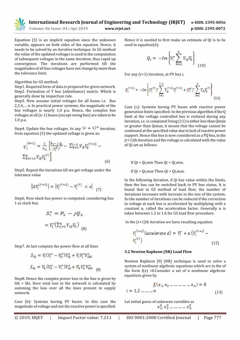
Equation (5) is an implicit equation since the unknown variable, appears on both sides of the equation. Hence, it needs to be solved by an iterative technique. In GS method the value of the updated voltages is used in the computation of subsequent voltages in the same iteration, thus rapid up convergence. The iterations are performed till the magnitudes of all bus voltages have not change by more than the tolerance limit.

Algorithm for GS method: Step1. Required form of data is prepared for given network. Step2. Formation of Y bus (admittance) matrix. Which is generally done by inspection rule. Step3. Now assume initial voltages for all buses i.e. Bus 2,3,4,… n. In practical power systems, the magnitude of the bus voltages is nearly 1.0 p.u. Hence, the complex bus voltages at all (n-1) buses (except swing bus) are taken to be 1.0 p.u.

Step4. Update the bus voltages. In any iteration, from equation (5) the updated voltage is given as:

(6)

Step5. Repeat the iterations till we get voltage under the tolerance value

(7)

Step6. Now slack bus power is computed, considering bus 1 as slack bus.

(8)

Step7. At last compute the power flow at all lines

(9)

Step8. Hence the complex power loss in the line is given by Sik + Ski. Here total loss in the network is calculated by summing the loss over all the lines present in supply network.

Case (b): Systems having PV buses: In this case the magnitude of voltage and not the reactive power is specified.

Hence it is needed to first make an estimate of Qi is to be used in equation(6).

(10)

For any (r+1) iteration, at PV bus i,

(11)

Case (c): Systems having PV buses with reactive power generation limits specified: In the previous algorithm if the Q limit at the voltage controlled bus is violated during any iteration, i.e. is computed Using (11) is either less than Qimin or greater than Qimax, it means that the voltage cannot be continued at the specified value due to lack of reactive power support. Hence this bus is now considered as a PQ bus, in the (r+1)th iteration and the voltage is calculated with the value of Qi set as follows:

If Qi < Qi,min Then Qi = Qi,min.

If Qi > Qi,max Then Qi = Qi,max.

In the following iteration, if Qi has value within the limits, then the bus can be switched back to PV bus status. It is found that in GS method of load flow, the number of iterations increases with increase in the size of the system. So the number of iterations can be reduced if the correction in voltage at each bus is accelerated by multiplying with a constant α, called the acceleration factor. Generally α is taken between 1.2 to 1.6 for GS load flow procedure.

In the (r+1)th iteration we have resulting equation

(12)

3.2 Newton Raphson (NR) Load Flow Newton Raphson [9] (NR) technique is used to solve a system of nonlinear algebraic equations which are in the of the form f(x) =0.Consider a set of n nonlinear algebraic equations given by

(13) Let initial guess of unknwon variables as




And the respective corrections value as

Thus we have

(14) Using Taylor’s series above equation can be expanded as

(15) Where i=1,2,3……..n, and higher order terms=0

By neglecting higher order derivative terms, the matrix form of equation (15) can be written as

(16) The vector form of above equation is given as

(17) Where jo is known as the Jacobian matrix , further the equation (17) can be written as

(18) The approximate values of corrections delta x can be obtained from equation (18). These being a set of linear algebraic equations. These can be solved efficiently by triangularisation of matrices back substitution. The updated values of x is given as

For (r+1)th iteration, in general it can be written as

(19) These iterations are continual till equation (13) is fulfilled to our desired accuracy i.e.

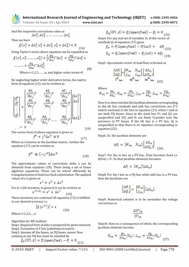
(20) Where i=1,2,3,….n Algorithm for NR method: Step1. Required form of data is prepared for given network. Step2. Formation of Y bus (admittance) matrix Step3. Assume all the buses, as PQ buses, power flow solution at any PQ bus must be satisfied by

(21)

(22) Step4. For any test set of variables Vi, δi the vector of residuals fo of equation (17) gives

(23)

(24)

Step5. Aproximate vector of load flow is formed as

(25)

Where

Now it is observed that the Jacobian elements corresponding to the ith bus residuals and mth bus corrections are 2*2 matrix enclosed in the box in equation (21) where i and m are both PQ buses. Since at the slack bus P1 and Q1 are unspecified and |Vi| and δi are fixed. Consider now the presence of PV buses. If the ith bus is a PV bus, Qi is unspecified so that there is no equation corresponding to equation (22).

Step6. So the jacobian elements are

(26)

Step7. For the m bus as a PV bus, |Vm| becomes fixed i.e. Δ|Vm| = 0 , So that Jacobian elements becomes

Step8. For the i bus as a PQ bus while mth bus is a PV bus, then the Jacobians are

Step9. Numerical solution is to be normalize the voltage corrections as

Step10. Now as a consequence of which, the corresponding jacobian elements become

(27)




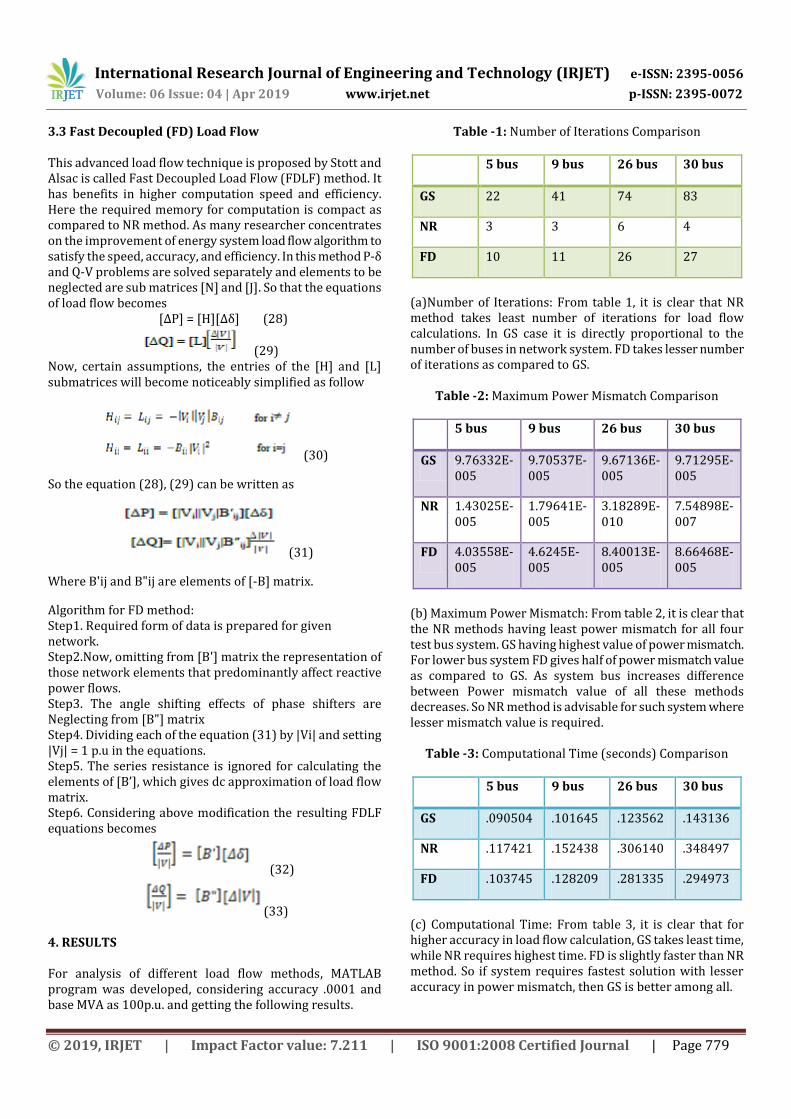
3.3 Fast Decoupled (FD) Load Flow This advanced load flow technique is proposed by Stott and Alsac is called Fast Decoupled Load Flow (FDLF) method. It has benefits in higher computation speed and efficiency. Here the required memory for computation is compact as compared to NR method. As many researcher concentrates on the improvement of energy system load flow algorithm to satisfy the speed, accuracy, and efficiency. In this method P-δ and Q-V problems are solved separately and elements to be neglected are sub matrices [N] and [J]. So that the equations of load flow becomes

[ΔP] = [H][Δδ] (28)

(29) Now, certain assumptions, the entries of the [H] and [L] submatrices will become noticeably simplified as follow

(30)

So the equation (28), (29) can be written as

(31)

Where Bʹij and Bʺij are elements of [-B] matrix.

Algorithm for FD method: Step1. Required form of data is prepared for given network. Step2.Now, omitting from [Bʹ] matrix the representation of those network elements that predominantly affect reactive power flows. Step3. The angle shifting effects of phase shifters are Neglecting from [Bʺ] matrix Step4. Dividing each of the equation (31) by |Vi| and setting |Vj| = 1 p.u in the equations. Step5. The series resistance is ignored for calculating the elements of [B’], which gives dc approximation of load flow matrix. Step6. Considering above modification the resulting FDLF equations becomes

(32)

(33) 4. RESULTS For analysis of different load flow methods, MATLAB program was developed, considering accuracy .0001 and base MVA as 100p.u. and getting the following results.

Table -1: Number of Iterations Comparison

5 bus 9 bus 26 bus 30 bus

GS 22 41 74 83

NR 3 3 6 4

FD 10 11 26 27

(a)Number of Iterations: From table 1, it is clear that NR method takes least number of iterations for load flow calculations. In GS case it is directly proportional to the number of buses in network system. FD takes lesser number of iterations as compared to GS.

Table -2: Maximum Power Mismatch Comparison


GS 9.76332E-005

9.70537E-005

9.67136E-005

9.71295E-005

NR 1.43025E-005

1.79641E-005

3.18289E-010

7.54898E-007

FD 4.03558E-005

4.6245E-005

8.40013E-005

8.66468E-005

(b) Maximum Power Mismatch: From table 2, it is clear that the NR methods having least power mismatch for all four test bus system. GS having highest value of power mismatch. For lower bus system FD gives half of power mismatch value as compared to GS. As system bus increases difference between Power mismatch value of all these methods decreases. So NR method is advisable for such system where lesser mismatch value is required.

Table -3: Computational Time (seconds) Comparison


GS .090504 .101645 .123562 .143136

NR .117421 .152438 .306140 .348497

FD .103745 .128209 .281335 .294973

(c) Computational Time: From table 3, it is clear that for higher accuracy in load flow calculation, GS takes least time, while NR requires highest time. FD is slightly faster than NR method. So if system requires fastest solution with lesser accuracy in power mismatch, then GS is better among all.




5. CONCLUSION Considering the above results, it is clear that the Newton-Raphson method is more reliable because it has less power penalty and less iteration than the other methods. In general, despite its longest computation time, the NR algorithm requires the least number of iterations to converge. However, as accuracy increases, the computation time of GS is much lower than other methods. The number of iterations for Gauss-Seidel increases directly with the number of buses in the network, while the number of iterations for the NR method remains virtually constant, regardless of the size of the system. However in FD method, because the convergence properties of the fast decoupling technique are geometrically related to NR quadratic convergence, it requires more iteration. Since, because of the high accuracy load flow obtained in a few systems only, the Newton-Raphson method is better to the use and more reliable than any other method. REFERENCES

[1] Hadi Saadat, (2006), “Power System Analysis”, McGraw-Hill.

[2] Nagrath, I.J and Kothari, D.P, (2006), Power System Engineering”, Tata McGraw-Hill Publishing Company Limited

[3] Ravi Kumar S.V. and Siva Nagaraju S (2007),”Loss Minimization by Incorporation of UPFC in Load Flow Analysis”, International Journal of Electrical and Power Engineering 1(3) page 321-327. Stagg, G.W. and EL- Abiad, A. H., (1968); “Computer Method in Power System Analysis”, McGraw- Hill, New York.

[4] Dharamjit, Tanti, D.K. (2012), “Load Flow Analysis on IEEE 30 bus System”, International Journal of Scientific and Research, Vol. 2, No. 11. Pp. 2250-3153

[5] Srikanth P., Rajendra O., Yesuraj A. and Tilak M., (2013), “Load Flow Analysis of IEEE 14 Bus System Using MATLAB”, International Journal of Engineering Research and Technology, Vol. 2, No. 5. Pp. 2278-0181

[6] Adejumobi I.A., Adepoju G.A. and Hamzat K.A. (2013), “Iterative Techniques for Load Flow Study”, Vol. 3 No. 1, Pp. 2249- 8958

[7] Gaganpreet Kaur, S. K Bath and B. S. Sidhu (2014), “Comparative Analysis of Load Flow Computational Methods Using MATLAB” International journal of

engineering research and technology, Vol. 3 Issue 4, April – 2014

[8] Kriti Singhal, (2014), “Load Flow Analysis Methods in Power System”, International Journal of Scientific & Engineering Research, Volume 5, Issue 5, May-2014

[9] Ashirwad Dubey, “Load flow analysis of power system”

International Journal of Scientific & Engineering Research, Volume 7, Issue 5, May-2016

[10] Ali M. Eltamaly and Amer Nasr A. Elghaffar, (2016)“Load Flow Analysis by Gauss-Seidel Method; A Survey” International Journal of Mechatronics, Electrical and

Computer Technology (IJMEC) Oct 2016

Documents

Comparative Analysis of Load Flow Methods on Standard Bus ...tested on standard IEEE 5, IEEE 9, IEEE 26 and IEEE 30 bus system. All methods have some advantages and disadvantages