COMP20010: Algorithms and Imperative Programming

COMP20010: Algorithms and Imperative Programming

Lecture 3Heaps

Dictionaries and Hash Tables

Lecture outline

The heap data structure; Implementing priority queues as heaps; The vector representation of a heap and

basic operations (insertion,removal); Heap-Sort; Dictionaries (the unordered dictionary ADT); Hash tables (bucket arrays, hash functions); Collision handling schemes;

The heap data structure

The aim is to provide a realisation of a priority queue that is efficient for both insertions and removals.

This can be accomplished with a data structure called a heap, which enables to perform both insertions and removals in logarithmic time.

The idea is to store the elements in a binary tree instead of a sequence.


A heap is a binary tree that stores a collection of keys at its internal nodes that satisfies two additional properties: A relational property (that affects how the keys are stored); A structural property;

We assume a total order relationship on the keys. Heap-Order property: In a heap T for every node v other than a

root, the key stored in v is greater or equal than the key stored at its parent.

The consequence is that the keys encountered on a path from the root to an external node are in non-decreasing order and that a minimum key is always stored at the root.

Complete binary tree property: A binary tree T with height h is complete if the levels 0 to h-1 have the maximum number of nodes (level i has nodes for i=0,…,h-1) and in the level h-1 all internal nodes are to the left of the external nodes.

i2


4

5 6

15 9 7 20

16 25

An example of a heap T storing 13 integer keys. The last node (the right-most, deepest internal node of T) is 8 in this case

14 12 11 8

Implementing a Priority Queue with a Heap

A heap-based priority queue consists of: heap: a complete binary tree with keys that satisfy the heap-

order property. The binary tree is implemented as a vector. last: A reference to the last node in T. For a vector

implementation, last is an integer index to the vector element storing the last node of T.

comp: A comparator that defines the total order relation among the keys. The comparator should maintain the minimal element at the root.

A heap T with n keys has height . If the update operations on a heap can be performed in time

proportional to its height, rather than to the number of its elements, then these operations will have complexity .

)1log( nh

)(lognO

Implementing a Priority Queue with a Heap

(4,C)

(5,A) (6,Z)

(15,K) (9,F) (7,Q) (20,B)

(16,X) (25,J) (14,E) (12,H) (11,S) (8,W)

heap

last

comp

<=>

Insertion into the PQ implemented with Heap

In order to store a new key-element pair (k,e) into T, we need to add a new node to T. To keep the complete tree property, the new node must become the last node of T.

If a heap is implemented as a vector, the insertion node is added at index n+1, where n is the current size of the heap.

Up-heap bubbling after an insertion

After the insertion of the element z into the tree T, it remains complete, but the heap-order property may be violated.

Unless the new node is the root (the PQ was empty prior to the insertion), we compare keys k(z) and k(u) where u is the parent of z. If k(u)>k(z), the heap order property needs to be restored, which can locally be achieved by swapping the pairs (u,k(u)) and (z,k(z)), making the element pair (z,k(z)) to go up one level. This upward movement caused by swaps is referred to as up-heap-bubbling.

In the worst case the up-heap-bubbling may cause the new element to move all the way to the root.

Thus, the worst case running time of the method insertItem is proportional to the height of T, i.e. , as T is complete.)(lognO

Up-heap bubbling after an insertion(an example)

(4,C)

(5,A) (6,Z)

(15,K) (9,F) (7,Q) (20,B)

(16,X) (25,J) (14,E) (12,H) (11,S) (8,W)


(4,C)

(5,A) (6,Z)

(15,K) (9,F) (7,Q) (20,B)

(16,X) (25,J) (14,E) (12,H) (11,S) (2,T)(8,W)


(4,C)

(5,A) (6,Z)

(15,K) (9,F) (7,Q)

(16,X) (25,J) (14,E) (12,H) (11,S) (8,W)

(20,B)

(2,T)


(4,C)

(5,A) (6,Z)

(15,K) (9,F) (7,Q) (2,T)

(16,X) (25,J) (14,E) (12,H) (11,S) (20,B)(8,W)


(4,C)

(5,A)

(15,K) (9,F) (7,Q)

(16,X) (25,J) (14,E) (12,H) (11,S) (20,B)(8,W)

(2,T)

(6,Z)


(4,C)

(5,A) (2,T)

(15,K) (9,F) (7,Q) (6,Z)

(16,X) (25,J) (14,E) (12,H) (11,S) (20,B)(8,W)


(5,A)

(15,K) (9,F) (7,Q) (6,Z)

(16,X) (25,J) (14,E) (12,H) (11,S) (20,B)(8,W)

(4,C)

(2,T)


(2,T)

(5,A) (4,C)

(15,K) (9,F) (7,Q) (6,Z)

(16,X) (25,J) (14,E) (12,H) (11,S) (20,B)(8,W)

Removal from the PQ implemented as a Heap

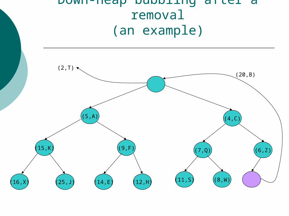
We need to perform the method removeMin from the PQ.

The element r with a smallest key is stored at the root of the heap. A simple deletion of this element would disrupt the binary tree structure.

We access the last node in the tree, copy it to the root, and delete it. This makes T complete.

However, these operations may violate the heap-order property.

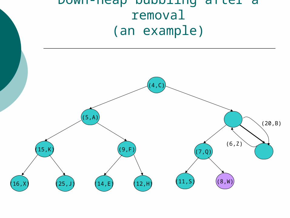
Removal from the PQ implemented as a Heap

To restore the heap-order property, we examine the root r of T. If this is the only node, the heap-order property is trivially satisfied. Otherwise, we distinguish two cases: If the root has only the left child, let s be the left child; Otherwise, let s be the child of r with the smallest key;

If k(r)>k(s), the heap-order property is restored by swapping locally the pairs stored at r and s.

We should continue swapping down T until no violation of the heap-order property occurs. This downward swapping process is referred to as down-heap bubbling. A single swap either resolves the violation of the heap-order property or propagates it one level down the heap.

The running time of the method removeMin is thus .)(lognO

Down-heap bubbling after a removal(an example)

(2,T)

(5,A) (4,C)

(15,K) (9,F) (7,Q) (6,Z)

(16,X) (25,J) (14,E) (12,H) (11,S) (20,B)(8,W)


(5,A) (4,C)

(15,K) (9,F) (7,Q) (6,Z)

(16,X) (25,J) (14,E) (12,H) (11,S) (20,B)(8,W)

(2,T)


(5,A) (4,C)

(15,K) (9,F) (7,Q) (6,Z)

(16,X) (25,J) (14,E) (12,H) (11,S) (8,W)

(2,T)(20,B)


(20,B)

(5,A) (4,C)

(15,K) (9,F) (7,Q) (6,Z)

(16,X) (25,J) (14,E) (12,H) (11,S) (8,W)


(5,A)

(15,K) (9,F) (7,Q) (6,Z)

(16,X) (25,J) (14,E) (12,H) (11,S) (8,W)

(20,B)

(4,C)


(4,C)

(5,A) (20,B)

(15,K) (9,F) (7,Q) (6,Z)

(16,X) (25,J) (14,E) (12,H) (11,S) (8,W)


(4,C)

(5,A)

(15,K) (9,F) (7,Q)

(16,X) (25,J) (14,E) (12,H) (11,S) (8,W)

(20,B)

(6,Z)


(4,C)

(5,A) (6,Z)

(15,K) (9,F) (7,Q) (20,B)

(16,X) (25,J) (14,E) (12,H) (11,S) (8,W)

Heap-Sort

Consider the PQ-Sort scheme that uses PQ to sort a sequence. If the PQ is implemented with a heap, during the insertion phase

each of n insertItem operations takes , where k is the number of elements currently in the heap.

During the second phase, each of n removeMin operations require time.

As at all times, the worst case run-time for each phase is equal to .

This gives a total run time of a PQ sort algorithm as if a heap is used to implement a PQ. This sorting algorithm is known as heap-sort. This is a considerable improvement from selection-sort and insertion sort that both require time.

If the sequence S to be sorted is implemented as an array, then heap-sort can be implemented in-place, using one part of the sequence to store the heap.

)(log kO

)(log kOnk

)(lognO)log( nnO

)( 2nO

Heap-Sort We use the heap with the largest element on top. During the

execution, left part of S (S[0:i-1]) is used to store the elements of the heap, and the right portion (S[i+1,n]). In the heap part of S, the element at the position k is greater or equal to its children at the positions 2k+1 and 2k+2.

In the first phase of the algorithm, we start with an empty heap, and move the boundary between the heap part and the sequence part from left to right one element at the time (at the step i we expand the heap by adding an element at the rank i-1.

In the second phase of the algorithm we start with an empty sequence and move the boundary between the heap and the sequence from right to left, one element at the time (at the step i we remove the maximum element from the heap and store it in the sequence part at the rank n-i.

Dictionaries and Hash Tables A computer dictionary is a data repository designed

to effectively perform the search operation. The user assigns keys to data elements and use them to search or add/remove elements.

The dictionary ADT has methods for the insertion, removal and searching of elements.

We store key-element pairs (k,e) called items into a dictionary.

In a student database (containing student’s name, address and course choices, for example) a key can be student’s ID.

There are two types of dictionaries: Unordered dictionaries; Ordered dictionarties;

Unordered dictionaries In the most general case we can allow multiple

elements to have the same key. However, in some applications this should not be advantageous (e.g. in a student database it would be confusing to have several different students with the same ID).

In the cases when keys are unique, a key associated to an object can be regarded as an address of this object. Such dictionaries are referred to as associative stores.

As an ADT a dictionary D supports the following methods: findElement(k) – if D contains an item with key k, return an

element e of such an item, else return an exception NO_SUCH_KEY.

insertItem(k,e) – insert an item with element e and key k in D RemoveElement(k) – remove from D an item with key k and

return its element, else return an exception NO_SUCH_KEY.

Log Files One simple way of realising an unordered dictionary

is by an unsorted sequence S, implemented itself by a vector or list that store (such implementation is referred to as a log file or audit trial).

This implementation is suitable for storing a small amount of data that do not change much over time.

With such implementation, the asymptotic execution times for dictionary methods are: insertItem – is implemented via insertLast method on S in

O(1) time; findElement – is performed by scanning the entire sequence

which takes O(n) in the worst case; removeElement – is performed by searching the whole

sequence until the element with the key k is found, again the worst case is O(n);

Hash Tables

If the keys represent the “addresses” of the elements, an effective way of implementing a dictionary is to use a hash table.

The main components of a hash table are the bucket arrays and the hash functions.

A bucket array for a hash table is an array A of size N, where each “element” of A is a container of key-element pairs, and N is the capacity of the array.

An element e with the key k is inserted into the bucket A[k].

If keys are not unique, two different elements may be mapped to the same bucket in A (a collision has occurred).

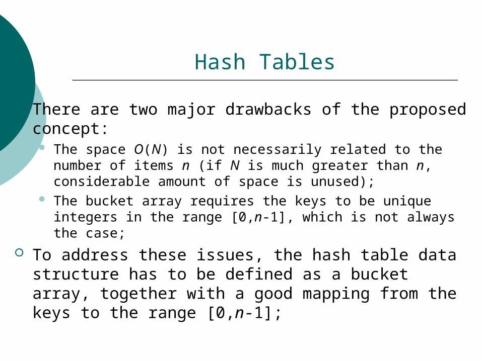
Hash Tables

There are two major drawbacks of the proposed concept: The space O(N) is not necessarily related to the number of

items n (if N is much greater than n, considerable amount of space is unused);

The bucket array requires the keys to be unique integers in the range [0,n-1], which is not always the case;

To address these issues, the hash table data structure has to be defined as a bucket array, together with a good mapping from the keys to the range [0,n-1];

Hash Functions

A hash function h maps each key k from a dictionary to an integer in range [0,N-1], where N is the bucket capacity.

Instead of using k as an index of the bucket array, we use h(k), i.e. we store the item (k,e) in the bucket A[h(k)].

A hash function is deemed to be “good” if it minimises collisions as much as possible, and at the same time eavaluating h(k) is not expensive.

The evaluation of a hash function consists of two phases: Mapping k to an integer (the hash code); Mapping the hash code to be an integer within the range of

indices in a bucket array (the compression map);

Hash Functions

k

hash code

-2 -1 0 1 2

compressionmap

0 1 N-1

Hash Codes

The first action performed on an (arbitrary) key k is to assign to it an integer value (called the hash code or hash value). This integer does not have to be in the range [0,N-1], but the algorithm for assigning it should avoid collisions.

If the range of values of k is larger than that assumed in the hash code (e.g. k is a long integer and the hash value is a short integer).

One way of creating a hash code in such situation is to take only lower or higher half of k as a hash code.

Another option is to sum lower and upper half of k (the summation hash code).

Polynomial Hash Codes

The summation hash code is not a good choice for keys that are character strings or other multiple-length objects of the form .

An example: Assume that ‘s are ASCII characters and that the hash code is defined as

Such approach would produce many unwanted collisions, such as:

),,,( 110 kxxx

ix

1

0

)ASCII()(k

iixkh

temp 01temp 10

topspotsstopspot

Polynomial Hash Codes A better hash code would take into account both the values

and their positions i. By choosing a constant , we can define the hash code:

This is a polynomial in a with the coefficients . Hence, this is the polynomial hash code. Experimental studies show that good spreads of hash codes are

obtained with certain choices for a (for example, 33,37,39,41); Tested on the case of 50,000 English words, each of these

choices provided fewer than 7 collisions.

ix)1,0( aa

122

11

0 kkkk xaxaxaxh

),,,( 110 kxxx

Compression Maps

If the range of hash codes generated for the keys exceeds the index range of the bucket array, the attempt to write the element would cause an out-of-bounds exception (either because the index is negative, or out of range [0,N-1].

The process of mapping an arbitrary integer to a range [0,N-1] is called compression, and is the second step in evaluating the hash function.

A compression map that uses:

is called the division method. If N is a prime number, the division compression map may help spreading out the hashed values. Otherwise, there is a likelihood that patterns in the key distributions are repeated (e.g. the keys {200,205,210,…,600} and N=100.

Nkkh mod)(

Compression Maps

A more sophisticated compression function is the multiply add and divide (or MAD method), with the compression function:

where N is a prime number, and a,b are random non-negative integers selected at the time of compression, such that

. With this choice of compression function the probability of

collision is at most 1/N.

Nbakh mod

0mod Na

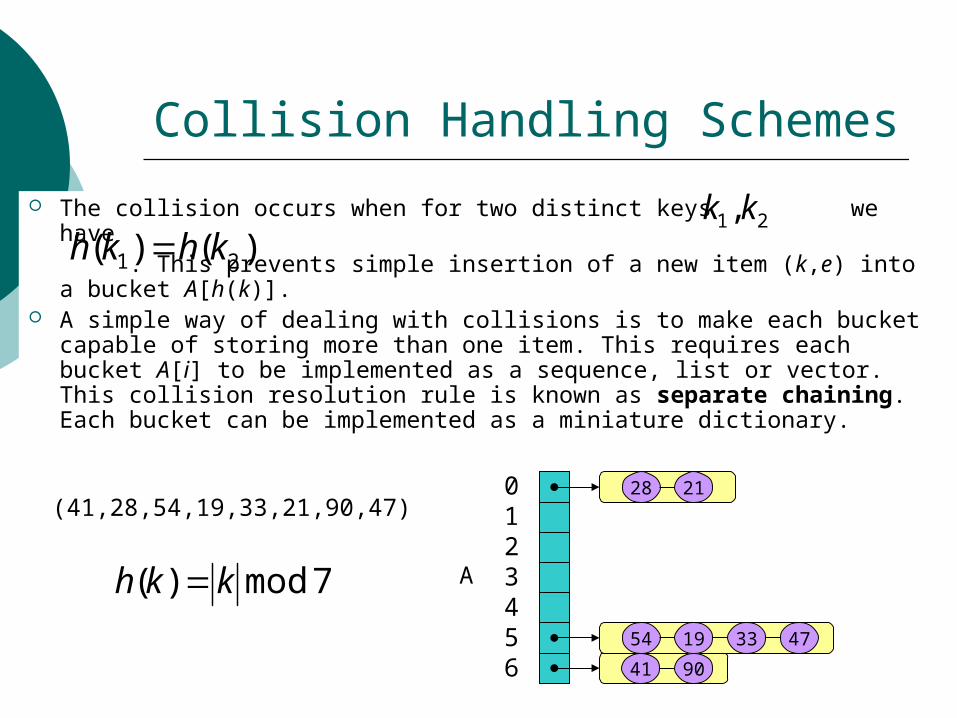
Collision Handling Schemes

The collision occurs when for two distinct keys we have

. This prevents simple insertion of a new item (k,e) into a bucket A[h(k)].

A simple way of dealing with collisions is to make each bucket capable of storing more than one item. This requires each bucket A[i] to be implemented as a sequence, list or vector. This collision resolution rule is known as separate chaining. Each bucket can be implemented as a miniature dictionary.

21,kk)()( 21 khkh

A

0123456 41

(41,28,54,19,33,21,90,47)

7mod)( kkh

28

54 19 33

21

90

47

Load Factors and Rehashing

If a good hashing function is used for storing n items of a dictionary in a bucket of size N, we expect each bucket to be of size ~n/N. This parameter (called load factor) should be kept small. If this requirement is fulfilled, the running time of methods findElement, insertItem and removeElement is

In order to keep the load factor below a constant the size of bucket array needs to be increased and to change the compression map. Then we need to re-insert all the existing hash table elements into a new bucket array using the new compression map. Such size increase and the hash table rebuild is called rehashing.

)/( NnO

Open Addressing

Separate chaining allows simple implementation of dictionary operations, but requires the use of an auxiliary data structure (a list, vector or sequence).

An alternative is to store only one element per bucket. This requires a more sophisticated approach of dealing with collisions.

Several methods for implementing this approach exist referred to as open addressing.

Linear Probing

In this strategy, if we try to insert an item (k,e) into a bucket A[h(k)]=A[i] that is already occupied, we try to insert an element in the positions A[(i+j)mod N] for j=1,2,… until a free place is found.

This approach requires re-implementation of the method findElement(k). To perform search we need to examine consecutive buckets starting from A[h(k)] until we either find an element or an empty bucket.

The operation removeElement(k) is more difficult to implement. The easiest way to implement it is to introduce a special “deactivated item” object.

With this object, findElement(k) and removeElement(k) should be implemented should skip over deactivated items and continue probing until a desired item or an empty bucket is found.

Linear Probing

The algorithm for inserItem(k,e) should stop at the deactivated item and replace it with e.

In conclusion, linear probing saves space, but complicates removals. It also clusters of a dictionary into contiguous runs, which slows down searches.

13 26 5 37 16 15

0 1 2 3

An insertion into a hash table with linear probing. The compression map is 11mod)( kkh

4 5 6 7 8 9 10

k=15

Quadratic Probing

Another open addressing strategy (known as quadratic probing) involves iterative attempts to buckets for j=0,1,2,… until an empty bucket is found.

It complicates the removal operation, but avoids clustering patterns characteristic with linear probing.

However, it creates secondary clustering with a set of secondary cells bouncing around a hash table in a fixed pattern.

If N is not a prime number, quadratic probing may fail to find an empty bucket, even if one exists. If the bucket array is over 50% full, this may happen even if N is a prime.

]mod)[( 2 NjiA

Double Hashing

Double hashing strategy eliminates the data clustering produced by the linear or quadratic probing.

In this approach a secondary hash function h’ is used. If the primary function h maps a key k to a bucket A[h(k)] that is already occupied, the the following buckets are attempted iteratively:

The second hash function must be non-zero. For N a prime number, the common choice is

with q<N a prime number. If memory size is not an issue, the separate chaining is always

competitive to collision handling schemes based on open addressing.

,...2,1))],([( jkhjiA

)mod()( qkqkh

Documents

COMP20010: Algorithms and Imperative Programming