COMP 515: Advanced Compilation for Vector and Parallel Processors

Vivek SarkarDepartment of Computer ScienceRice Universityvsarkar@rice.edu

http://www.cs.rice.edu/~vsarkar/comp515

COMP 515 Lecture 5 6 September, 2011

1

Acknowledgments• Slides from previous offerings of COMP 515 by Prof. Ken

Kennedy—http://www.cs.rice.edu/~ken/comp515/

2

MIV Dependences

Allen and Kennedy, Chapter 3

Section 3.3.3 to end

3

Recall from last time• General Dependence:

—Let (D1, D2, …, Dn) be a direction vector, and consider the following loop nest

DO i1 = L1, U1!

! ! ! ! DO i2 = L2, U2! ! ! ! ! !

! ! ! ! ! …! ! ! ! ! ! ! !

! ! ! ! ! DO in = Ln, Un! ! ! ! !

! ! S1 ! ! ! A(f(i)) = …! ! ! !

! ! S2 ! ! ! … = A(g(i))

ENDDO

! ! ! ! …

! ! ! ENDDO

Then S2 δ S1 if f(x) = f(y) can be solved for iteration vectors x,y that agree with D.

4

More Recall• Last time we cared about cases where f and g each involved a

single induction variable.

• There were several special cases that helped matters:– Strong SIV– Weak-zero SIV– Weak-crossing SIV

5

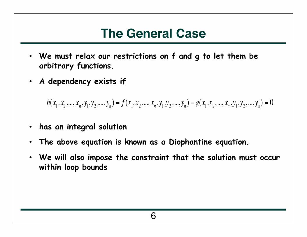
h(x1, x2 ,..., xn, y1,y2 ,..., yn ) = f (x1, x2, ..., xn ,y1,y2 , ..., yn ) − g(x1,x2, ..., xn ,y1,y2, ..., yn) = 0

The General Case• We must relax our restrictions on f and g to let them be

arbitrary functions.

• A dependency exists if

• has an integral solution

• The above equation is known as a Diophantine equation.

• We will also impose the constraint that the solution must occur within loop bounds

6

• For simplicity, assume that

• Then, we’re looking for a solution of

• Rearranging terms, we get the linear Diophantine Equation:

f (x) = a0 + a1x1 + ... + anxng(x) = b0 + b1y1 + ... + bnyn

h(x) = a0 − b0 + a1x1 − b1y1 + ... + anxn − bnyn = 0

a1x1 − b1y1 + ... + anxn − bnyn = b0 − a0

Linear Diophantine Equations

7

Linear Diophantine Equations

• A basic result tells us that there are values for x1,x2,…,xn,y1,y2,…,yn so that

What’s more, gcd(a1,…,an,b1,…,bn) is the smallest number this is true for.

• As a result, the equation has a solution iff gcd(a1,…,an,b1,…,bn) divides b0 - a0

— But the solution may not be in the region (loop iteration values) of interest

• Exercise: try this result on the A(4*i+2) & A(4*i+4) example

a1x1 − b1y1 + ... + anxn − bnyn = gcd(a1, ..., an, b1, ..., bn)

8

Real Solutions• Unfortunately, the gcd test is less useful then it might seem.

• Useful technique is to show that the equation has no solutions in region of interest ==> explore real solutions for this purpose

• Solving h(x) = 0 is essentially an integer programming problem. Linear programming techniques are used as an approximation.

• Since the function is continuous, the Intermediate Value Theorem says that a solution exists iff:

€

minR h ≤ 0 ≤maxR h

9

Banerjee Inequality

• We need an easy way to calculate minR h and maxR h.

• Definitions:

• a+ and a- are also called the positive part and negative part of a, so that a = a+ - a-

€

hi+ =maxRi h(xi,yi)

€

hi− =minRi h(xi,yi)

a+ =a a ≥ 00 a < 0⎧ ⎨ ⎩

a− =a a < 00 a ≥ 0⎧ ⎨ ⎩

10

Banerjee Inequality• Lemma 3.2. Let t,l,u,z be real numbers. If l <= z <= u, then

Furthermore, there are numbers z1 and z2 in [l,u] that make each of the inequalities true.

Proof: In the book.

−t −u + t +l ≤ tz ≤ t +u − t −l

11

Banerjee Inequality

• Definitions:—Hi

-(<) = -(ai- + b)+(Ui -1) + [(ai

- + bi)- +ai+]Li - bi

—Hi+(<) = (ai

+ - bi)+(Ui- 1) - [(ai+ - bi)++ ai

-]Li- bi

—Hi-(=) = -(ai - bi)-Ui + (ai - bi)+Li

—Hi+(=) = (ai - bi)+Ui - (ai - bi)-Li

—Hi-(>) = -(ai - bi)-(Ui - 1) + [(ai - bi

+)+ + bi-]Li + ai

—Hi+(>) = (ai + bi)+(Ui - 1) - [(ai + bi

-)- + bi+]Li + ai

—Hi-(*) = ai

-Uix + ai

+Lix - bi

+Uiy + bi

-Liy

—Hi+(*) = ai

+Uix - ai

-Lix + bi

-Uiy - bi

+Liy

12

Banerjee Inequality• Now for the main lemma:

• Lemma 3.3: Let D be a direction vector, and h be a dependence function. Let hi(xi,yi) = aixi -biyi and Ri be as described above. Then hi obtains its minimum and maximum on Ri, and we have

min Ri hi = hi− = Hi

−(Di)

max Ri hi = hi+ = Hi

+(Di )

13

Banerjee Inequality• Proof of 3.3:

We must check for all cases of Di .

If Di = ‘=‘, then xi=yi and hi=(ai-bi) xi. We clearly satisfy the hypothesis of lemma 3.2, so

Furthermore, hi actually obtains these bounds by lemma 3.2. Thus, the result is established.

−(ai − bi )−Ui + (ai − bi )

+ Li = Hi−(=) ≤ h ≤ (ai − bi)

+Ui − (ai − bi)− Li = Hi

+(=)

14

Banerjee Inequality If Di = ‘<“, we have that Li <= xi < yi <= Ui. Rewrite this as Li <= xi

<= yi -1 <= Ui - 1 in order to satisfy the conditions for lemma 3.2. Also, rewrite h as

Then, we can use 3.2 to first minimize aixi and get:

Minimizing the bi(yi-1) term then gives us:

The other cases are similar.

hi = aixi − biyi = aixi − bi(yi −1) − bi

−ai−(yi −1) + ai

+Li − bi(yi −1) − bi ≤ hi ≤ ai+(yi −1) − ai

−Li − bi(yi −1) − bi

−(ai− + bi )

+(Ui −1) + (ai− + bi)

− Li + ai+ Li − bi = Hi

−(<) ≤ hi≤ (ai+ − bi)+(Ui −1) − (ai+ − bi)− Li − ai− Li − bi = Hi

+(<)

15

Banerjee Inequality• Theorem 3.3 (Banerjee). Let D be a direction vector, and h be

a dependence function. h = 0 can be solved in the region R iff:

Proof: Immediate from Lemma 3.3 and the IMV.

Hi−(Di) ≤ b0 − a0 ≤

i=1

n

∑ Hi+(Di)

i=1

n

∑

16

ExampleDO I = 1, N

DO J = 1, M

DO K = 1, 100

A(I,K) = A(I+J,K) + B

ENDDO

ENDDO

ENDDO

Testing (I, I+J) for D = (=,<,*):

This is impossible, so the dependency doesn’t exist.

H1−(=) + H2

−(<) = −(1− 0)−N + (1−1)+1 − (0− +1)+(M −1) + [(0− +1)− + 0+]1− 1 = −M ≤ 0≤ H1+(=) + H2+ (<) = (1 −1)+ N − (1 −1)−1+ (0+ −1)+ (M − 1) − [(0+ −1)− + 0−]1 −1 ≤ −2

17

Trapezoidal Banerjee Test• Banerjee test assumes that all loop indices are independent.

• In practice, this is often not true.

• Banerjee will always report a dependency if it does exist.

• Banerjee may, however, report a dependence if none exists.

18

Trapezoidal Banerjee Test• Assume that:

• Now, our bounds must change. For example:

Ui =Ui 0 + Uijijj=1

i−1

∑

Li = Li0 + Lijijj=1

i−1

∑

Hi−(<) = −(ai

− + bi )+ Ui 0 −1 + Uijyj

j=1

i−1

∑⎛

⎝ ⎜ ⎜

⎞

⎠ ⎟ ⎟ + (ai

− + bi)− Li0 + Lijyj

j=1

i−1

∑⎛

⎝ ⎜ ⎜

⎞

⎠ ⎟ ⎟

+ai+ Li 0 + Lijx jj=1

i−1

∑⎛

⎝ ⎜ ⎜

⎞

⎠ ⎟ ⎟ − bi

19

Testing Direction Vectors• Must test pair of statements for all direction vectors.

• Potentially exponential in loop nesting.

• Can save time by pruning:

(<,<,*)

(<,=,<) (<,=,=) (<,>,=)

(<,=,*) (<,>,*)

(<,*,*) (=,*,*) (>,*,*)

(*,*,*)

20

Coupled Groups

• So far, we’ve assumed separable subscripts.

• We can glean information from separable subscripts, and use it to split coupled groups.

• Most subscripts tend to be SIV, so this works pretty well.

21

Delta Test• Constraint vector C for a subscript group, contains one

constraint for each index in group.

• The Delta test derives and propagates constraints from SIV subscripts.

• Constraints are also propagated from Restricted Double Index Variable (RDIV) subscripts, those of the form

• See Figure 3.13 in textbook for Delta test algorithm

< a1i + c1,a2 j + c2 >

22

Delta Test Example! ! DO I

! ! ! DO J

! ! ! ! DO K

! ! ! ! ! A(J-I, I+1, J+K) = A(J-I,I,J+K)

! ! ! ! ENDDO

! ! ! ENDDO

! ! ENDDO

• The delta test gives us a distance vector of (1,1,-1) for this loop nest.

• First pass: establish ∆I = 1 from second dimension

• Second pass: Propagate into first dimension to obtain ∆J = 1

• Third pass: Propagate into third dimension to obtain ∆K = -1

23

Final Assembly• Basic dependence algorithm (for a given direction vector):

Figure out what sort of subscripts we have

! ! Partition subscripts into coupled groups

! ! for each separable subscript

! ! ! test it using appropriate test

! ! ! if no dependence, we’re done

! ! for each coupled group

! ! ! use delta test

! ! ! if no dependence, we’re done

! ! return dependence

• For more advanced dependence tests, see the Omega Project (http://www.cs.umd.edu/projects/omega/)

24

Preliminary Transformations

Chapter 4 of Allen and Kennedy

25

Overview• Why do we need this?

—Requirements of dependence testing– Stride 1– Normalized loop– Linear subscripts– Subscripts composed of functions of loop induction variables

—Higher dependence test accuracy—Easier implementation of dependence tests

26

An Example

INC = 2KI = 0DO I = 1, 100 DO J = 1, 100 KI = KI + INC U(KI) = U(KI) + W(J) ENDDO S(I) = U(KI)ENDDO

• Programmers optimized code—Confusing to smart compilers

27

An Example

INC = 2KI = 0DO I = 1, 100 DO J = 1, 100 ! Deleted: KI = KI + INC U(KI + J*INC) = U(KI + J*INC) + W(J) ENDDO KI = KI + 100 * INC S(I) = U(KI)ENDDO

• Applying induction-variable substitution—Replace references to induction variables with functions of loop

index for the purpose of dependence analysis

28

An Example

INC = 2KI = 0DO I = 1, 100 DO J = 1, 100 U(KI + (I-1)*100*INC + J*INC) = U(KI + (I-1)*100*INC + J*INC) + W(J) ENDDO ! Deleted: KI = KI + 100 * INC S(I) = U(KI + I * (100*INC))ENDDOKI = KI + 100 * 100 * INC

• Second application of IVS—Remove all references to KI

29

An Example

INC = 2! Deleted: KI = 0DO I = 1, 100 DO J = 1, 100 U(I*200 + J*2 - 200) = U(I*200 + J*2 -200) + W(J) ENDDO S(I) = U(I*200)ENDDOKI = 20000

• Applying Constant Propagation—Substitute the constants

30

An Example

DO I = 1, 100 DO J = 1, 100 U(I*200 + J*2 - 200) = U(I*200 + J*2 - 200) + W(J) ENDDO S(I) = U(I*200)ENDDO

• Applying Dead Code Elimination—Removes all unused code

31

Information Requirements• Transformations need knowledge

—Loop Stride—Loop-invariant quantities—Constant-values assignment—Usage of variables

32

Loop Normalization• Transform loop so that

—The new stride becomes +1 (more important)—The new lower bound becomes +1 (less important)

• To make dependence testing as simple as possible

• Serves as information gathering phase

33

Loop Normalization

• Caveat— Un-normalized:

DO I = 1, M DO J = I, N

A(J, I) = A(J, I - 1) + 5

ENDDO ENDDO

Has a direction vector of (<,=)

— Normalized:

DO I = 1, M DO J = 1, N – I + 1

A(J + I – 1, I) = A(J + I – 1, I – 1) + 5 ENDDO

ENDDO

Has a direction vector of (<,>)

34

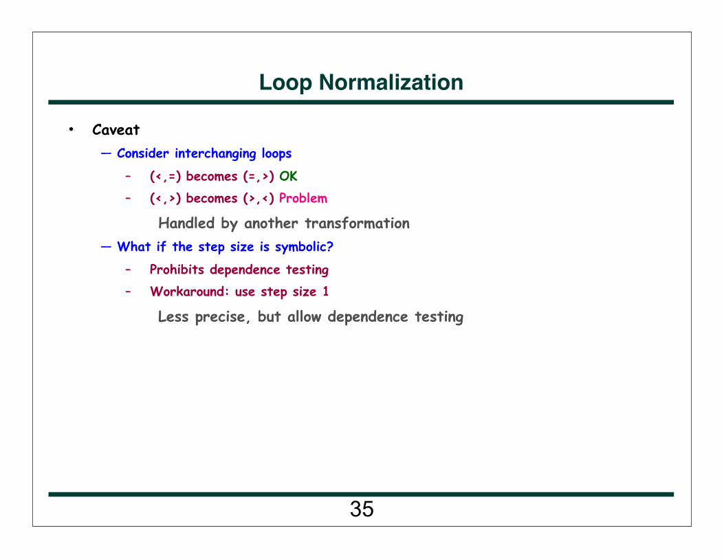
Loop Normalization

• Caveat— Consider interchanging loops

– (<,=) becomes (=,>) OK– (<,>) becomes (>,<) Problem

Handled by another transformation— What if the step size is symbolic?

– Prohibits dependence testing– Workaround: use step size 1

Less precise, but allow dependence testing

35