Embed Size (px)
Citation preview

Ergod. Th. & Dynam. Sys. (First published online 2019), page 1 of 26∗
doi:10.1017/etds.2019.51 c© Cambridge University Press, 2019∗Provisional—final page numbers to be inserted when paper edition is published
Commuting rational functions revisited
FEDOR PAKOVICH
Department of Mathematics, Ben Gurion University, P.O. Box 653,Beer Sheva, 8410501, Israel
(e-mail: [email protected])
(Received 15 February 2019 and accepted in revised form 12 June 2019)
Abstract. Let B be a rational function of degree at least two that is neither a Lattes mapnor conjugate to z±n or ±Tn . We provide a method for describing the set CB consisting ofall rational functions commuting with B. Specifically, we define an equivalence relation∼B
on CB such that the quotient CB/∼B
possesses the structure of a finite group G B , and
describe generators of G B in terms of the fundamental group of a special graph associatedwith B.
Key words: commuting rational functions, the Ritt theorem, common iterates
2010 Mathematics Subject Classification: 30D05 (Primary); 37F10 (Secondary)
1. IntroductionIn this paper, we study commuting rational functions, that is rational solutions of thefunctional equation
B ◦ X = X ◦ B. (1)
More precisely, we fix a function B ∈ C(z) of degree at least two and study the set CB
consisting of all X ∈ C(z) such that (1) holds.Functional equation (1) has been investigated previously by Julia [3] and Fatou [2].
In particular, they showed that commuting rational functions X and B of degree at leasttwo have the same Julia set J = J (X)= J (B). Using Poincare functions, Julia and Fatouproved that if X and B have no iterate in common and J 6= CP1, then, up to a conjugacy,X and B are either powers or Chebyshev polynomials. The assumption J 6= CP1 wasremoved by Ritt [13], who used a topological-algebraic method. Ritt proved that solutionsof (1) having no iterate in common reduce to powers, to Chebyshev polynomials, or toLattes maps. A proof of the Ritt theorem based on modern dynamical methods was givenby Eremenko [1].

2 F. Pakovich
All the above results assume that X and B have no iterate in common. However,commuting rational functions X and B such that
B◦l = X◦k (2)
for some l, k ≥ 1 also exist. The simplest examples of such functions can be obtained bysetting
X = R◦l1 , B = R◦l2 ,
where R is an arbitrary rational function and l1, l2 ≥ 1. More generally, denoting byAut(R) the group of Mobius transformations commuting with R, we can set
X = µ1 ◦ R◦l1 , B = µ2 ◦ R◦l2 , (3)
where µ1 and µ2 are elements of Aut(R) commuting between themselves. However, it hasbeen shown already by Ritt [13] that commuting rational functions satisfying (2) are notexhausted by functions of the form (3). Although Ritt’s method provides some insight intothe structure of commuting rational functions X and B satisfying (2), it does not permitthe description of this class of functions in an explicit way, and Ritt concluded his paperby saying: ‘we think that the example given above makes it conceivable that no great ordermay reign in this class’.
Functional equation (1) is a particular case of the functional equation
A ◦ X = X ◦ B, (4)
where A and B are rational functions of degree at least two. In case that (4) is satisfiedfor some rational function X of degree at least two, the function B is called semiconjugateto the function A. Semiconjugate rational functions were investigated in the recent papers[5, 6, 8–10]. In particular, it was shown in [6] that solutions of (4) satisfying C(X, B)=C(z), called primitive, can be described in terms of group actions on CP1 or C, implyingstrong restrictions on a possible form of A, B and X . Any solution of (4) reduces to aprimitive one by a certain iterative process, and the quantitative aspects of this reductionwere studied in [5]. In particular, it was shown in [5] that if a rational function B is notspecial, that is, if B is neither a Lattes map nor conjugate to z±n or ±Tn , then solutions ofequations (1) and (4) obey some finiteness conditions.
Specifically, with regards to equation (1), it was shown in [5] that if B is not special,then there exist finitely many rational functions X1, X2, . . . , Xr such that X commuteswith B if and only if
X = Xj ◦ B◦k
for some j , 1≤ j ≤ r , and k ≥ 0. Moreover, the number r and the degrees of Xj ,1≤ j ≤ r , can be bounded by numbers depending on deg B only. Note that this resultimmediately implies the Ritt theorem. Indeed, if X commutes with B, then any iterateX◦l , l ≥ 1, does. Thus, by the Dirichlet box principle, there exist distinct l1, l2 such that
X◦l1 = Xj ◦ B◦k1 , X◦l2 = Xj ◦ B◦k2
for the same j and some k1, k2 ≥ 0. Therefore, if, say, l2 > l1, then
X◦l2 = X◦l1 ◦ B◦k2−k1 ,
implying that (2) holds for l = l2 − l1 and k = k2 − k1, since X and B commute.

Commuting rational functions revisited 3
In this paper, we provide a method for describing the set CB for non-special B. Forsuch B, essentially all the information about CB provided by the Ritt method reduces tothe fact that any element of CB has a common iterate with B. Thus, new approaches andtechniques are needed, and we develop them in this paper. Our main results are as follows.First, for any non-special rational function B, we define an equivalence relation ∼
Bon the
set CB such that the quotient CB/∼B
possesses the structure of a finite group G B . Second,
we describe generators of this group in terms of the fundamental group of a special graphassociated with B, providing a method for describing CB . Finally, we calculate G B forseveral classes of rational functions. Note that our method of describing CB reduces theproblem to the easier problem of finding all functional decompositions F =U ◦ V forfinitely many rational functions F .
In more detail, for a non-special rational function B, we define an equivalence relation∼B
on the set CB , setting A1 ∼B
A2 if
A1 ◦ B◦l1 = A2 ◦ B◦l2
for some l1 ≥ 0, l2 ≥ 0, and show that the multiplication of classes induced by thefunctional composition of their representatives provides CB/∼
Bwith the structure of a
finite group G B . The group structure on CB/∼B
offers a new look at the problem of
describing CB , and permits the characterization of properties of CB in group theoreticterms. For example, the group G B is trivial if and only if any element of CB is an iterate ofB, while G B is isomorphic to Aut(B) if and only if any element of CB can be representedin the form X = µ ◦ Bk , where µ ∈ Aut(B) and k ≥ 0.
We describe generators of G B using a special finite graph 0B defined as follows. Let Bbe a rational function. We say that a rational function B is an elementary transformationof B if there exist rational functions U and V such that B = V ◦U and B =U ◦ V . Wesay that rational functions B and A are equivalent and write A ∼ B if there exists a chainof elementary transformations between B and A (this equivalence relation should not beconfused with the previous one where the subscript B is used). Since for any Mobiustransformation µ the equality
B = (B ◦ µ−1) ◦ µ
holds, the equivalence class [B] of a rational function B is a union of conjugacy classes.Moreover, by the result of [9], the class [B] consists of finitely many conjugacy classes,unless B is a flexible Lattes map. The graph 0B is defined as a multigraph whose verticesare in a one-to-one correspondence with some fixed representatives Bi of conjugacy classesin [B], and whose multiple edges connecting the vertices corresponding to Bi to B j are ina one-to-one correspondence with solutions of the system
Bi = V ◦U, B j =U ◦ V
in rational functions. In these terms, the main result of the paper about the group G B is aconstruction of a group epimorphism from the fundamental group of the graph 0B to thegroup G B .
The paper is organized as follows. In §2, we describe the set CB in terms of elementarytransformations. In §3, we define the group G B . In §§4 and 5, we define the graph 0B
4 F. Pakovich
and construct a group epimorphism from π1(0B) to G B . We also show that if A ∼ B, thenthe groups G A and G B are isomorphic. Note that this implies, in particular, that if A is arational function such that the group Aut(A) is non-trivial, then for any rational functionB ∼ A the group G B is also non-trivial, even though Aut(B) can be trivial. In the last case,functions of degree one in CA give rise to functions of higher degree in CB through theisomorphism G A ∼= G B .
In §6, we calculate the group G B for certain classes of rational functions, and considersome examples. Specifically, we show that for a wide class of rational functions, whichwe call generically decomposable, G B is isomorphic to Aut(B). We also show that fora polynomial B the group G B is metacyclic. Finally, we discuss in detail the example ofcommuting rational functions B and X satisfying condition (2) from the paper of Ritt [13].In particular, we calculate the group G B that turns out to be a cyclic group of order three.We also provide a different example of this kind.
2. The set CB and elementary transformationsLet B be a rational function of degree at least two. We denote by CB the set of all rationalfunctions commuting with B.
LEMMA 2.1. The set CB is closed with respect to the operation of composition, thatis, A1, A2 ∈ CB implies A1 ◦ A2 ∈ CB . Furthermore, if A ◦U ∈ CB and U ∈ CB , thenA ∈ CB .
Proof. Indeed, if A1, A2 ∈ CB , then
A1 ◦ A2 ◦ B = A1 ◦ B ◦ A2 = B ◦ A1 ◦ A2.
On the other hand, if A ◦U ∈ CB and U ∈ CB , then
B ◦ A ◦U = A ◦U ◦ B = A ◦ B ◦U,
implying thatB ◦ A = A ◦ B. �
We emphasize that we allow to elements of CB to have degree one, that is to be Mobiustransformations. All Mobius transformations commuting with B obviously form a groupdenoted by Aut(B) and called the symmetry group of B. Since any µ ∈ Aut(B) mapsperiodic points of B of order l ≥ 1 to themselves, and any Mobius transformation is definedby its values at any three points, the symmetry group of any rational function is finite. Inparticular, Aut(B) is one of the five well-known finite rotation groups of the sphere: A4,S4, A5, Cn , D2n . Note that the property of µ ∈ Aut(B) to map periodic points of B toperiodic points can be used for a practical description of Aut(B).
Let B be a rational function. A rational function B is called an elementarytransformation of B if there exist rational functions U and V such that B = V ◦U andB =U ◦ V . We say that rational functions B and A are equivalent and write A ∼ B ifthere exists a chain of elementary transformations between B and A. Since for any Mobiustransformation µ the equality
B = (B ◦ µ−1) ◦ µ
Commuting rational functions revisited 5
holds, the equivalence class [B] of a rational function B is a union of conjugacy classes.Thus, the relation∼ can be considered as a weaker form of the classical conjugacy relation.The equivalence class [B] contains infinitely many conjugacy classes if and only if B is aflexible Lattes map [9].
The following lemma is obtained by a direct calculation (see [10, Lemma 3.1]).
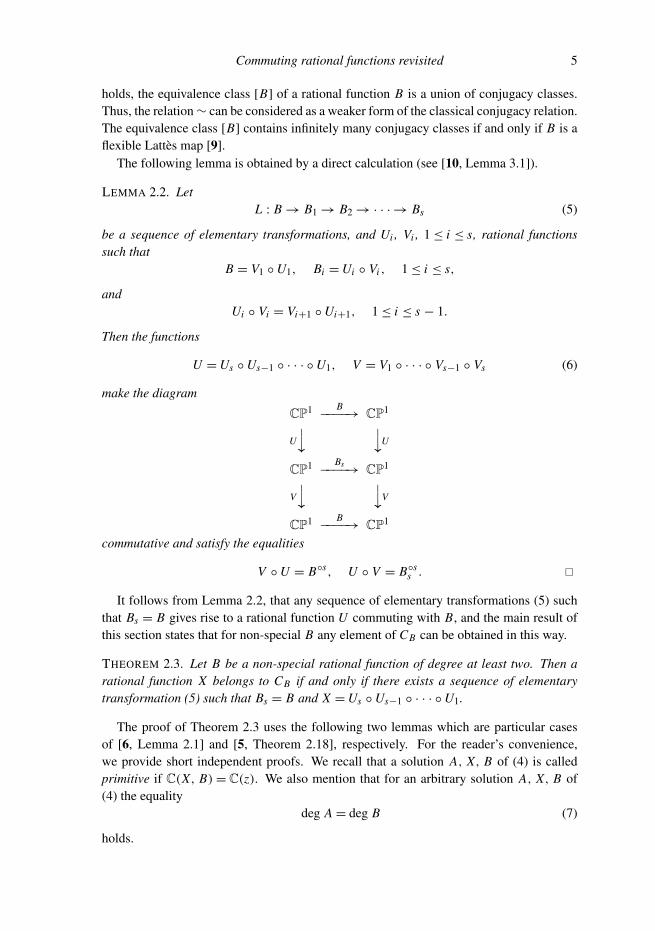
LEMMA 2.2. LetL : B→ B1→ B2→ · · · → Bs (5)
be a sequence of elementary transformations, and Ui , Vi , 1≤ i ≤ s, rational functionssuch that
B = V1 ◦U1, Bi =Ui ◦ Vi , 1≤ i ≤ s,
andUi ◦ Vi = Vi+1 ◦Ui+1, 1≤ i ≤ s − 1.
Then the functions
U =Us ◦Us−1 ◦ · · · ◦U1, V = V1 ◦ · · · ◦ Vs−1 ◦ Vs (6)
make the diagram
CP1 B−−−−→ CP1
U
y yU
CP1 Bs−−−−→ CP1
V
y yV
CP1 B−−−−→ CP1
commutative and satisfy the equalities
V ◦U = B◦s, U ◦ V = B◦ss . �
It follows from Lemma 2.2, that any sequence of elementary transformations (5) suchthat Bs = B gives rise to a rational function U commuting with B, and the main result ofthis section states that for non-special B any element of CB can be obtained in this way.
THEOREM 2.3. Let B be a non-special rational function of degree at least two. Then arational function X belongs to CB if and only if there exists a sequence of elementarytransformation (5) such that Bs = B and X =Us ◦Us−1 ◦ · · · ◦U1.
The proof of Theorem 2.3 uses the following two lemmas which are particular casesof [6, Lemma 2.1] and [5, Theorem 2.18], respectively. For the reader’s convenience,we provide short independent proofs. We recall that a solution A, X, B of (4) is calledprimitive if C(X, B)= C(z). We also mention that for an arbitrary solution A, X, B of(4) the equality
deg A = deg B (7)
holds.

6 F. Pakovich
LEMMA 2.4. A solution A, X, B of (4) is primitive if and only if the algebraic curve
A(x)− X (y)= 0 (8)
is irreducible.
Proof. By the Luroth theorem, there exists a rational function W such that C(X, B)=C(W ), implying that the equalities
X = X ′ ◦W, B = B ′ ◦W (9)
hold for some rational functions X ′ and B ′ with C(X ′, B ′)= C(z). Clearly, x = X ′(t),y = B ′(t) is a generically one-to-one parametrization of some irreducible component
C : F(x, y)= 0
of (8). Furthermore, since the degree of the projection of C on x (respectively, y) is equalto deg X ′ (respectively, deg B ′) the equalities
degx F = deg B ′, degy F = deg X ′ (10)
hold. If C(X, B)= C(z), then deg W = 1, and it follows from equalities (9), (10), and (7)that the curve C coincides with curve (8), implying that (8) is irreducible. On the otherhand, if C(X, B) 6= C(z), then deg W > 1, and equalities (9), (10), and (7) imply that C isa proper component of (8). �
LEMMA 2.5. Let A, X, B be a primitive solution of (4). Then for any l ≥ 1, the solutionA◦l , X, B◦l is also primitive.
Proof. The proof is by induction on l. For l = 1, the lemma is trivially true. Assume thatit is true for all k ≤ l. By Lemma 2.4, this implies that the algebraic curve
Ck : A◦k(x)− X (y)= 0
is irreducible for all k ≤ l, and
Rk : x = X (t), y = B◦k(t)
is its generically one-to-one parametrization.Let P1, P2 be arbitrary rational functions satisfying the equality
A◦(l+1)◦ P1 = X ◦ P2. (11)
Since the curve Cl is irreducible and Rl is its generically one-to-one parametrization, theequality
A◦(l+1)◦ P1 = A◦l ◦ (A ◦ P1)= X ◦ P2
implies thatA ◦ P1 = X ◦W, P2 = B◦l ◦W
for some W ∈ C(z). Furthermore, since the curve C1 is also irreducible, it follows fromthe first of these equalities that
P1 = X ◦U, W = B ◦U

Commuting rational functions revisited 7
for some U ∈ C(z). Thus, any pair of rational functions P1, P2 satisfying (11) has theform
P1 = X ◦U, P2 = B◦(l+1)◦U
for some U ∈ C(z). In particular, this implies that if the equalities
X = P1 ◦W, B◦(l+1)= P2 ◦W (12)
hold for some P1, P2, W ∈ C(z), then deg W = 1, since P1, P2 in (12) satisfy (11).Therefore, C(X, B◦(l+1))= C(z), that is, A◦(l+1), X, B◦(l+1) is a primitive solution. �
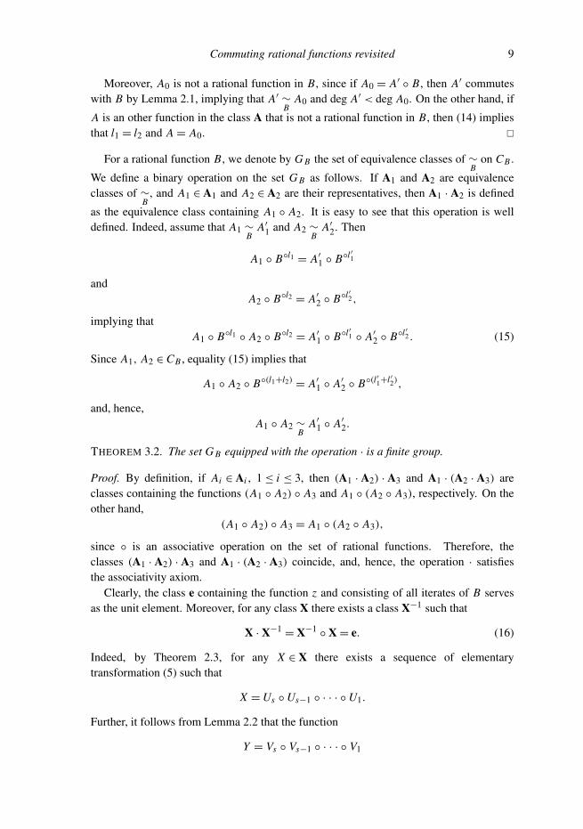
Proof of Theorem 2.3. The sufficiency follows from Lemma 2.2. In the other direction,assume that X ∈ CB . If X is a Mobius transformation, then the sequence
B = (B ◦ X−1) ◦ X→ X ◦ (B ◦ X−1)= B
is as required. Thus, assume that deg X ≥ 2.We observe first that there exist a sequence (5) and a commutative diagram
CP1 B−−−−→ CP1
U
y yU
CP1 Bs−−−−→ CP1
X0
y yX0
CP1 B−−−−→ CP1
such that U is defined by (6), the equality X = X0 ◦U holds, and the triple B, X0, Bs isa primitive solution of (4). Indeed, if B, X, B is a primitive solution of (4), we can setU = z, X0 = X , and Bs = B. Otherwise, C(X, B)= C(W ) for some W with deg W > 1,and substituting equalities (9) in (4) we see that the diagram
CP1 B−−−−→ CP1
W
y yW
CP1 W◦B′−−−−→ CP1
X ′y yX ′
CP1 B−−−−→ CP1
commutes. If the solution B, X ′, W ◦ B ′ of (4) is primitive, we are done. Otherwise, wecan apply the above transformation to this solution. Since deg X ′ < deg X , it is clear thatafter a finite number of steps we obtain a sequence of elementary transformations (5) andfunctions U , X0, and Bs as required.
To prove Theorem 2.3, we only must show that deg X0 = 1. Indeed, in this casechanging Us to X0 ◦Us and Bs to X0 ◦ Bs ◦ X−1
0 , without loss of generality we mayassume that X0 = z, so that Bs = B and (5) is the sequence required. Assume, in contrast,that deg X0 > 1. By Lemma 2.5, for any l ≥ 1 the triple B◦l , X0, B◦ls is a primitive solution

8 F. Pakovich
of (4). On the other hand, by the Ritt theorem, there exist k and l such that equality (2)holds. Thus,
B◦l = X◦k = X0 ◦ (U ◦ X◦k−1),
implying that the curve(U ◦ X◦k−1)(x)− y = 0
is a component of the curveB◦l(x)− X0(y)= 0.
Moreover, this component is proper because deg X0 > 1. Since, by Lemma 2.4, thiscontradicts the fact that B◦l , X0, B◦ls is a primitive solution of (4), we conclude thatdeg X0 = 1. �
3. The group G B
Define an equivalence relation ∼B
on the set CB , setting A1 ∼B
A2 if
A1 ◦ B◦l1 = A2 ◦ B◦l2 (13)
for some l1 ≥ 0, l2 ≥ 0 (in order to distinguish this relation from the relation ∼ introducedin the previous section we use the subscript B). It is easy to see that ∼
Bis really an
equivalence relation. Indeed, ∼B
is clearly reflexive and symmetric. Furthermore, if
equalities (13) andA2 ◦ B◦n1 = A3 ◦ B◦n2
hold, and n1 ≥ l2, then
A1 ◦ B◦(l1+n1−l2) = A2 ◦ B◦n1 = A3 ◦ B◦n2 ,
implying that A1 ∼B
A3. Similarly, if l2 ≥ n1, then
A3 ◦ B◦(n2+l2−n1) = A2 ◦ B◦l2 = A1 ◦ B◦l1 .
LEMMA 3.1. Let A be an equivalence class of ∼B
. For any n ≥ 1, the class A contains at
most one rational function of degree n. Furthermore, if A0 ∈ A is a function of minimalpossible degree, then any A ∈ A has the form A = A0 ◦ B◦l , l ≥ 1. Alternatively, thefunction A0 can be described as a unique function in A that is not a rational functionin B.
Proof. If deg A1 = deg A2 in (13), then l1 = l2, implying that A1 = A2. Furthermore, if
A ◦ B◦l1 = A0 ◦ B◦l2 (14)
and l1 > l2, thenA0 = A ◦ B◦(l1−l2),
implying that deg A < deg A0 in contradiction with the assumption. Therefore, l1 ≤ l2and, hence,
A = A0 ◦ B◦(l2−l1).
Commuting rational functions revisited 9
Moreover, A0 is not a rational function in B, since if A0 = A′ ◦ B, then A′ commuteswith B by Lemma 2.1, implying that A′ ∼
BA0 and deg A′ < deg A0. On the other hand, if
A is an other function in the class A that is not a rational function in B, then (14) impliesthat l1 = l2 and A = A0. �
For a rational function B, we denote by G B the set of equivalence classes of ∼B
on CB .
We define a binary operation on the set G B as follows. If A1 and A2 are equivalenceclasses of ∼
B, and A1 ∈ A1 and A2 ∈ A2 are their representatives, then A1 · A2 is defined
as the equivalence class containing A1 ◦ A2. It is easy to see that this operation is welldefined. Indeed, assume that A1 ∼
BA′1 and A2 ∼
BA′2. Then
A1 ◦ B◦l1 = A′1 ◦ B◦l′
1
andA2 ◦ B◦l2 = A′2 ◦ B◦l
′
2 ,
implying thatA1 ◦ B◦l1 ◦ A2 ◦ B◦l2 = A′1 ◦ B◦l
′
1 ◦ A′2 ◦ B◦l′
2 . (15)
Since A1, A2 ∈ CB , equality (15) implies that
A1 ◦ A2 ◦ B◦(l1+l2) = A′1 ◦ A′2 ◦ B◦(l′
1+l ′2),
and, hence,A1 ◦ A2 ∼
BA′1 ◦ A′2.
THEOREM 3.2. The set G B equipped with the operation · is a finite group.
Proof. By definition, if Ai ∈ Ai , 1≤ i ≤ 3, then (A1 · A2) · A3 and A1 · (A2 · A3) areclasses containing the functions (A1 ◦ A2) ◦ A3 and A1 ◦ (A2 ◦ A3), respectively. On theother hand,
(A1 ◦ A2) ◦ A3 = A1 ◦ (A2 ◦ A3),
since ◦ is an associative operation on the set of rational functions. Therefore, theclasses (A1 · A2) · A3 and A1 · (A2 · A3) coincide, and, hence, the operation · satisfiesthe associativity axiom.
Clearly, the class e containing the function z and consisting of all iterates of B servesas the unit element. Moreover, for any class X there exists a class X−1 such that
X · X−1= X−1
◦ X= e. (16)
Indeed, by Theorem 2.3, for any X ∈ X there exists a sequence of elementarytransformation (5) such that
X =Us ◦Us−1 ◦ · · · ◦U1.
Further, it follows from Lemma 2.2 that the function
Y = Vs ◦ Vs−1 ◦ · · · ◦ V1

10 F. Pakovich
belongs to CB , and the functions X and Y satisfy
X ◦ Y = Y ◦ X = B◦s .
Therefore, condition (16) holds for X−1 defined as the class containing the rationalfunction Y .
Finally, by the result of [5] cited in the introduction, there exist at most finitely manyrational functions A ∈ CB which are not rational functions in B, implying by Lemma 3.1that the group G B is finite. �
Note that the above proof provides a method for the actual finding X−1. On the otherhand, merely the existence of the inverse element follows from the Ritt theorem. Indeed,since for any X ∈ X there exist l, k ≥ 1 such that (2) holds, for any class X there existsk such that Xk
= e, implying that (16) holds for X−1= Xk−1. Note also that the Ritt
theorem by itself does not imply that the group G B is finite, although it does imply thatany its element has finite order.
For X ∈ CB , we denote by X the element of G B corresponding to the equivalence classof ∼
Bcontaining X .
LEMMA 3.3. The map µ→ µ is a group monomorphism from the group Aut(B) to thegroup G B .
Proof. Since functions from Aut(B) have degree one, it follows from Lemma 3.1 thatµ1 = µ2 if and only if µ1 = µ2. Therefore, the map τ : µ→ µ is injective, and it is easyto see that τ is a homomorphism of groups. �
We denote the image of Aut(B) in G B under the group monomorphism µ→ µ byAutG(B).
LEMMA 3.4. The following conditions are equivalent.(1) Any X ∈ CB has the form X = µ ◦ B◦l for some µ ∈ Aut(B) and l ≥ 0.(2) Any X ∈ CB of degree at least two is a rational function in B.(3) The group G B coincides with AutG(B).
Proof. It is easy to see that (1) and (3) are equivalent, and that (1) implies (2). Assumenow that (2) holds, and let X ∈ CB be a function of degree at least two. By the assumption,X = R1 ◦ B for some R ∈ C(z). Moreover, since by Lemma 2.1 the function R1 belongsto CB , using (2) again we conclude that either R1 ∈ Aut(B), or there exists R2 ∈ C(z) suchthat R1 = R2 ◦ B and R2 ∈ CB . It is clear that continuing this process we will eventuallyobtain a representation X = µ ◦ Bl for some µ ∈ Aut(B) and l ≥ 1. �
4. The graph 0B
Let B be a rational function of degree at least two. Define 0B as a multigraphwhose vertices are in a one-to-one correspondence with some fixed representatives ofconjugacy classes in [B], and whose multiple edges connecting vertices corresponding torepresentatives Bi and B j are in a one-to-one correspondence with solutions of the system
Bi = V ◦U, B j =U ◦ V (17)

Commuting rational functions revisited 11
in rational functions. Note that 0B have loops. They correspond to solutions of
Bi =U ◦ V = V ◦U.
LEMMA 4.1. The graph 0B does not depend on the choice of representatives of conjugacyclasses in [B].
Proof. Indeed, for any Mobius transformations α and β, to a solution U, V of system (17)corresponds a solution
U ′ = β ◦U ◦ α−1, V ′ = α ◦ V ◦ β−1 (18)
of the systemα ◦ Bi ◦ α
−1= V ′ ◦U ′, β ◦ B j ◦ β
−1=U ′ ◦ V ′. (19)
Furthermore, it is easy to see that formulas (18) provide a one-to-one correspondencebetween solutions of (17) and (19). �
THEOREM 4.2. Let B a rational function of degree at least two. Then the graph 0B isfinite, unless B is a flexible Lattes map.
Proof. By the main result of the paper [9], the class [B] contains infinitely many conjugacyclasses if and only if B is a flexible Lattes map. Therefore, if B is not such a map, the graph0B contains only finitely many vertices.
Let us show now that the number of edges connecting two vertices is finite. Recall thattwo decompositions
B = V ◦U, B = V ′ ◦U ′ (20)
of a rational function B into compositions of rational functions are called equivalent ifthere exists a Mobius transformation µ such that
V ′ = V ◦ µ−1, U ′ = µ ◦U. (21)
It is well known that equivalence classes of decompositions of B are in one-to-onecorrespondence with imprimitivity systems of the monodromy group Mon(B) of B. Inparticular, there exist at most finitely many such classes. Therefore, to prove the finitenessof the number of edges adjacent to the vertices corresponding to Bi and B j it is enough toshow that for any fixed solution U, V of (17) there exist only finitely many solutions U ′,V ′ of (17) such that decompositions (20) are equivalent. Since equalities (21) combinedwith the equality
U ◦ V =U ′ ◦ V ′
imply the equalityU ◦ V = µ ◦U ◦ V ◦ µ−1,
the last statement follows from the finiteness of the group Aut(U ◦ V ). �
Since in this paper we consider only non-special rational functions B, the correspondinggraphs 0B are always finite by Theorem 4.2. Note that the results of [5] imply that thenumber of vertices of 0B can be bounded by a number depending on deg B only (see [5,Remark 5.2]). Nevertheless, there exists no absolute bound for the number of vertices

12 F. Pakovich
FIGURE 1. The form of 0B in Example 1.
of 0B , and it is easy to construct rational functions B of degree n for which the graph 0B
contains ≈ log2 n vertices (see [6, p. 1241]).We always assume that the representative of the conjugacy class of the function B in
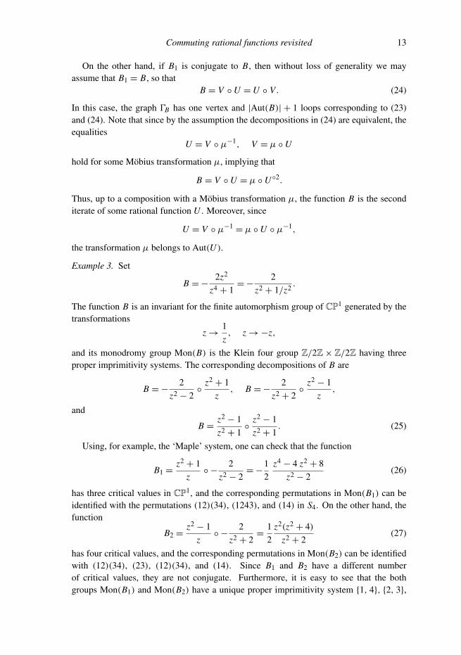
0B is the function B itself. Abusing notation, in the following we call the functions B j
simply ‘vertices’ of 0B . Note that for each vertex B j of 0B there exists at least one loopstarting and ending at B that corresponds to the solution
B = B ◦ z = z ◦ B (22)
of (17). More generally, the solutions
B = (µ−1◦ B) ◦ µ= µ ◦ (µ−1
◦ B), µ ∈ Aut(B), (23)
give rise to |Aut(B)| loops.
Example 1. Assume that B is an indecomposable rational function. By definition, thismeans that the equality B = V ◦U implies that at least one of the functions U and Vhas degree one. In this case, the equivalence class [B] obviously consists of a uniqueconjugacy class. Thus, 0B has a unique vertex, and all edges of 0B are loops correspondingto solutions of
B =U ◦ V = V ◦U
such that one of the functions U , V has degree one. Assuming without loss of generalitythat deg U = 1, we see that
B ◦U =U ◦ V ◦U =U ◦ B,
implying that U ∈ Aut(B). Therefore, 0B has the form shown in Figure 1, and the numberof loops of 0B is equal to |Aut(B)|.
Example 2. Assume now that a rational function B has, up to equivalency (21), a uniquedecomposition B = V ◦U into a composition of rational functions of degree at least two,and that the same is true for the function B1 =U ◦ V . In this case, graph 0B may havetwo distinct forms. Namely, if B1 and B are not conjugate, then 0B has the form shownin Figure 2, where all loops correspond to some automorphisms. Note that for such B andB1 the groups Aut(B) and Aut(B1) are isomorphic (see Lemma 6.3), implying that B andB1 have the same number of attached loops.
FIGURE 2. The form of 0B in Example 2.
Commuting rational functions revisited 13
On the other hand, if B1 is conjugate to B, then without loss of generality we mayassume that B1 = B, so that
B = V ◦U =U ◦ V . (24)
In this case, the graph 0B has one vertex and |Aut(B)| + 1 loops corresponding to (23)and (24). Note that since by the assumption the decompositions in (24) are equivalent, theequalities
U = V ◦ µ−1, V = µ ◦U
hold for some Mobius transformation µ, implying that
B = V ◦U = µ ◦U◦2.
Thus, up to a composition with a Mobius transformation µ, the function B is the seconditerate of some rational function U . Moreover, since
U = V ◦ µ−1= µ ◦U ◦ µ−1,
the transformation µ belongs to Aut(U ).
Example 3. Set
B =−2z2
z4 + 1=−
2z2 + 1/z2 .
The function B is an invariant for the finite automorphism group of CP1 generated by thetransformations
z→1z, z→−z,
and its monodromy group Mon(B) is the Klein four group Z/2Z× Z/2Z having threeproper imprimitivity systems. The corresponding decompositions of B are
B =−2
z2 − 2◦
z2+ 1z
, B =−2
z2 + 2◦
z2− 1z
,
and
B =z2− 1
z2 + 1◦
z2− 1
z2 + 1. (25)
Using, for example, the ‘Maple’ system, one can check that the function
B1 =z2+ 1z◦ −
2z2 − 2
=−12
z4− 4 z2
+ 8z2 − 2
(26)
has three critical values in CP1, and the corresponding permutations in Mon(B1) can beidentified with the permutations (12)(34), (1243), and (14) in S4. On the other hand, thefunction
B2 =z2− 1z◦ −
2z2 + 2
=12
z2(z2+ 4)
z2 + 2(27)
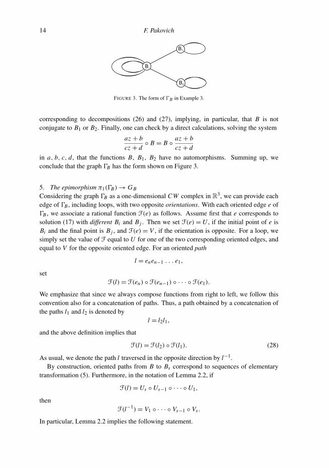
has four critical values, and the corresponding permutations in Mon(B2) can be identifiedwith (12)(34), (23), (12)(34), and (14). Since B1 and B2 have a different numberof critical values, they are not conjugate. Furthermore, it is easy to see that the bothgroups Mon(B1) and Mon(B2) have a unique proper imprimitivity system {1, 4}, {2, 3},
14 F. Pakovich
FIGURE 3. The form of 0B in Example 3.
corresponding to decompositions (26) and (27), implying, in particular, that B is notconjugate to B1 or B2. Finally, one can check by a direct calculations, solving the system
az + bcz + d
◦ B = B ◦az + bcz + d
in a, b, c, d , that the functions B, B1, B2 have no automorphisms. Summing up, weconclude that the graph 0B has the form shown on Figure 3.
5. The epimorphism π1(0B)→ G B
Considering the graph 0B as a one-dimensional CW complex in R3, we can provide eachedge of 0B , including loops, with two opposite orientations. With each oriented edge e of0B , we associate a rational function F(e) as follows. Assume first that e corresponds tosolution (17) with different Bi and B j . Then we set F(e)=U , if the initial point of e isBi and the final point is B j , and F(e)= V , if the orientation is opposite. For a loop, wesimply set the value of F equal to U for one of the two corresponding oriented edges, andequal to V for the opposite oriented edge. For an oriented path
l = enen−1 . . . e1,
setF(l)= F(en) ◦ F(en−1) ◦ · · · ◦ F(e1).
We emphasize that since we always compose functions from right to left, we follow thisconvention also for a concatenation of paths. Thus, a path obtained by a concatenation ofthe paths l1 and l2 is denoted by
l = l2l1,
and the above definition implies that
F(l)= F(l2) ◦ F(l1). (28)
As usual, we denote the path l traversed in the opposite direction by l−1.By construction, oriented paths from B to Bs correspond to sequences of elementary
transformation (5). Furthermore, in the notation of Lemma 2.2, if
F(l)=Us ◦Us−1 ◦ · · · ◦U1,
thenF(l−1)= V1 ◦ · · · ◦ Vs−1 ◦ Vs .
In particular, Lemma 2.2 implies the following statement.

Commuting rational functions revisited 15
LEMMA 5.1. Let l be an oriented path in 0B from the vertex B to a vertex Bs consistingof k oriented edges. Then
Bs ◦ F(l)= F(l) ◦ B, (29)
andF(l−1) ◦ F(l)= B◦k, F(l) ◦ F(l−1)= B◦ks . � (30)
If l is a closed path in 0B starting and ending at B, then (29) implies that the functionF(l) commutes with B, while equalities (30) reduce to the equalities
F(l−1) ◦ F(l)= F(l) ◦ F(l−1)= B◦k . (31)
Thus, we obtain a map φB : l→ F(l) from the set of closed paths starting and ending atB to the set CB .
THEOREM 5.2. The map φB : l→ F(l) descends to an epimorphism of groups 8B :
π1(0B, B)→ G B .
Proof. Let 0 be a graph. Recall that an oriented path l in 0 is called reduced if no twosuccessive oriented edges in l are opposite orientations of the same edge. Paths of the forme−1e, where e is an oriented edge are called spurs. Paths l and l ′ are called equivalent if l ′ isobtained from l by a finite number of insertions and removals of spurs between successiveoriented edges or at the endpoints. In these terms, the fundamental group π1(0, V ) of thegraph 0 can be defined as the set of equivalence classes of paths that begin and end atsome fixed vertex V of 0, equipped with the product of classes defined in an obvious way(see e.g. [14, §2.1.6]).
To prove that the map φB descends to a map from π1(0B, B) to G B , we must show thatwhenever closed paths l and l ′ in 0B that start and end at B are equivalent, the rationalfunctions F(l) and F(l ′) are in the same equivalence class of CB . Since any path isequivalent to a path with no spurs, for this purpose it is enough to show that if l ′ is obtainedfrom l by an insertion of a spur, then F(l)∼
BF(l ′). Assume that
l ′ = l2e−1el1,
where l1 is a path from B to Bs , and l2 is a path from Bs to B (one of the paths l1 and l2can be empty in which case Bs = B). Then
F(l ′)= F(l2) ◦ Bs ◦ F(l1),
by (28) and (31). It follows now from (29) that
F(l ′)= F(l2) ◦ F(l1) ◦ B = F(l) ◦ B,
implying that F(l)∼BF(l ′). Thus, φB descends to a map 8B : π1(0B, B)→ G B , and (28)
implies that 8B is a homomorphism of groups.Finally, it follows from Theorem 2.3 that 8B is an epimorphism. Indeed, by Theorem
2.3, any X ∈ CB can be obtained from a sequence of elementary transformations (5).Moreover, we can change if necessary each of rational functions Bi , 1≤ i ≤ s − 1,appearing in (5) to any desired representative of its conjugacy class, consecutively

16 F. Pakovich
changing the function Ui to αi ◦Ui , the function Bi to αi ◦ Bi ◦ α−1i , and the function Ui+1
to α−1i ◦Ui+1 for a convenient Mobius transformation αi . Therefore, for any X ∈ CB ,
there exists a closed path l starting and ending at B such that F(l)= X , implying that8B : π1(0B, B)→ G B is an epimorphism. �
THEOREM 5.3. Let A and B be equivalent rational functions. Then G B ∼= G A.
Proof. Assuming that A and B are vertices of 0B , take a path s from A to B in 0B . Sincethe map ψ : l→ s−1ls, from the set of closed paths starting and ending at B to the setof closed paths starting and ending at A, descends to an isomorphism of the fundamentalgroups
9 : π1(0B, B)→ π1(0B, A),
it follows from Theorem 5.2 that we only need to prove the equality
9(Ker8B)= Ker8A. (32)
Let l0 be a path starting and ending at B such that F(l0)= B◦k , k ≥ 1, and let k0 =
ψ(l0). ThenF(k0)= F(s−1) ◦ F(l0) ◦ F(s)= F(s−1) ◦ B◦k ◦ F(s),
implying by (29) and (30) that
F(k0)= F(s−1) ◦ F(s) ◦ A◦k = A◦l ◦ A◦k = A◦(k+l)
for some k, l ≥ 1. This implies that
9(Ker8B)⊆ Ker8A.
Similarly, considering the isomorphism inverse to 9 we obtain that
9−1(Ker8A)⊆ Ker8B .
This proves equality (32). �
6. Examples of groups G B
6.1. Functions with G B = AutG(B). The simplest application of Theorem 5.2 is thefollowing result.
THEOREM 6.1. Let B be an indecomposable non-special rational function of degree atleast two. Then G B = AutG(B). Equivalently, X ∈ CB if and only if X = µ ◦ Bl for someµ ∈ Aut(B) and l ≥ 1.
Proof. Since 0B has a unique vertex and |Aut(B)| loops corresponding to automorphismsof B (see Example 1), it follows easily from Theorem 5.2 that G B is generated by µ,µ ∈ Aut(B). Thus, G B = AutG(B). The second statement follows from Lemma 3.4. �
Note that Theorem 6.1 implies that for a ‘random’ rational function B, the group G B istrivial, since such a function is indecomposable and has no automorphisms.
Theorem 6.1 can be extended to a wide class of decomposable rational functions. Recallthat a functional decomposition
B =Ur ◦Ur−1 ◦ · · · ◦U1 (33)
Commuting rational functions revisited 17
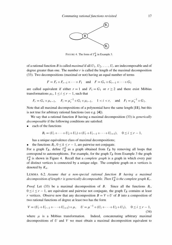
FIGURE 4. The form of 00B in Example 3.
of a rational function B is called maximal if all U1,U2, . . . ,Ur are indecomposable and ofdegree greater than one. The number r is called the length of the maximal decomposition(33). Two decompositions (maximal or not) having an equal number of terms
F = Fr ◦ Fr−1 ◦ · · · ◦ F1 and F = Gr ◦ Gr−1 ◦ · · · ◦ G1
are called equivalent if either r = 1 and F1 = G1 or r ≥ 2 and there exist Mobiustransformations µi , 1≤ i ≤ r − 1, such that
Fr = Gr ◦ µr−1, Fi = µ−1i ◦ Gi ◦ µi−1, 1< i < r, and F1 = µ
−11 ◦ G1.
Note that all maximal decompositions of a polynomial have the same length [11], but thisis not true for arbitrary rational functions (see e.g. [4]).
We say that a rational function B having a maximal decomposition (33) is genericallydecomposable if the following conditions are satisfied:• each of the functions
Bi = (Ui ◦ · · · ◦U2 ◦U1) ◦ (Ur ◦Ur−1 ◦ · · · ◦Ui+1), 0≤ i ≤ r − 1,
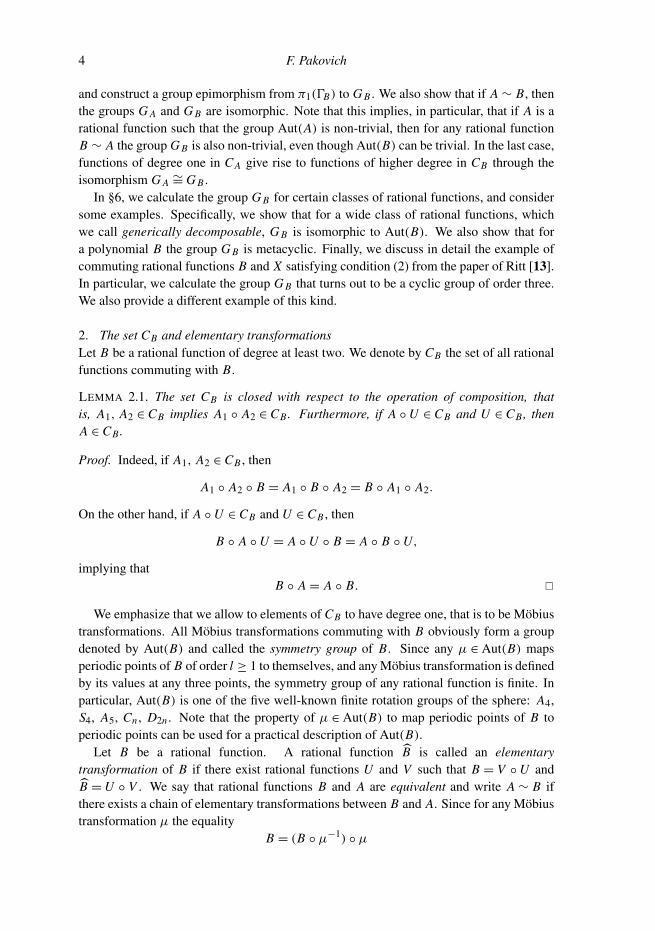
has a unique equivalence class of maximal decompositions;• the functions Bi , 0≤ k ≤ r − 1, are pairwise not conjugate.For a graph 0B , define 00
B as a graph obtained from 0B by removing all loops thatcorrespond to automorphisms. For example, for the graph 0B from Example 3 the graph00
B is shown in Figure 4. Recall that a complete graph is a graph in which every pairof distinct vertices is connected by a unique edge. The complete graph on n vertices isdenoted by Kn .
LEMMA 6.2. Assume that a non-special rational function B having a maximaldecomposition of length r is generically decomposable. Then 00
B is the complete graph Kr .
Proof. Let (33) be a maximal decomposition of B. Since all the functions Bi ,0≤ i ≤ r − 1, are equivalent and pairwise not conjugate, the graph 0B contains at leastr vertices. Observe now that any decomposition B = V ◦U of B into a composition oftwo rational functions of degree at least two has the form
V = (Ur ◦Ur−1 ◦ · · · ◦Ui+1) ◦ µ, U = µ−1◦ (Ui ◦ · · · ◦U2 ◦U1), 0≤ i ≤ r − 1,
(34)where µ is a Mobius transformation. Indeed, concatenating arbitrary maximaldecompositions of U and V we must obtain a maximal decomposition equivalent to
18 F. Pakovich
(33), implying that (34) holds. Therefore, any edge of 0B adjacent to B0 = B andnot corresponding to an automorphism of B is adjacent to one of the vertices Bi ,1≤ k ≤ r − 1, and there exists exactly one edge connecting B0 and Bi , 1≤ k ≤ r − 1.Since the same argument holds for any Bi , 0≤ k ≤ r − 1, we conclude that 00
B is thecomplete graph Kr . �
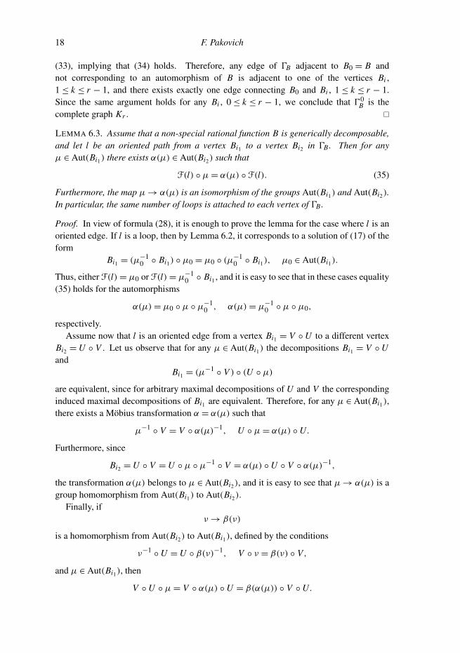
LEMMA 6.3. Assume that a non-special rational function B is generically decomposable,and let l be an oriented path from a vertex Bi1 to a vertex Bi2 in 0B . Then for anyµ ∈ Aut(Bi1) there exists α(µ) ∈ Aut(Bi2) such that
F(l) ◦ µ= α(µ) ◦ F(l). (35)
Furthermore, the map µ→ α(µ) is an isomorphism of the groups Aut(Bi1) and Aut(Bi2).In particular, the same number of loops is attached to each vertex of 0B .
Proof. In view of formula (28), it is enough to prove the lemma for the case where l is anoriented edge. If l is a loop, then by Lemma 6.2, it corresponds to a solution of (17) of theform
Bi1 = (µ−10 ◦ Bi1) ◦ µ0 = µ0 ◦ (µ
−10 ◦ Bi1), µ0 ∈ Aut(Bi1).
Thus, either F(l)= µ0 or F(l)= µ−10 ◦ Bi1 , and it is easy to see that in these cases equality
(35) holds for the automorphisms
α(µ)= µ0 ◦ µ ◦ µ−10 , α(µ)= µ−1
0 ◦ µ ◦ µ0,
respectively.Assume now that l is an oriented edge from a vertex Bi1 = V ◦U to a different vertex
Bi2 =U ◦ V . Let us observe that for any µ ∈ Aut(Bi1) the decompositions Bi1 = V ◦Uand
Bi1 = (µ−1◦ V ) ◦ (U ◦ µ)
are equivalent, since for arbitrary maximal decompositions of U and V the correspondinginduced maximal decompositions of Bi1 are equivalent. Therefore, for any µ ∈ Aut(Bi1),there exists a Mobius transformation α = α(µ) such that
µ−1◦ V = V ◦ α(µ)−1, U ◦ µ= α(µ) ◦U.
Furthermore, since
Bi2 =U ◦ V =U ◦ µ ◦ µ−1◦ V = α(µ) ◦U ◦ V ◦ α(µ)−1,
the transformation α(µ) belongs to µ ∈ Aut(Bi2), and it is easy to see that µ→ α(µ) is agroup homomorphism from Aut(Bi1) to Aut(Bi2).
Finally, ifν→ β(ν)
is a homomorphism from Aut(Bi2) to Aut(Bi1), defined by the conditions
ν−1◦U =U ◦ β(ν)−1, V ◦ ν = β(ν) ◦ V,
and µ ∈ Aut(Bi1), then
V ◦U ◦ µ= V ◦ α(µ) ◦U = β(α(µ)) ◦ V ◦U.

Commuting rational functions revisited 19
SinceV ◦U ◦ µ= µ ◦ V ◦U,
this implies that β ◦ α is the identical mapping of Aut(Bi1), and hence µ→ α(µ) is anisomorphism. �
THEOREM 6.4. Let B be a non-special generically decomposable rational function. ThenG B = AutG(B). Equivalently, X ∈ CB if and only if X = µ ◦ Bl for some µ ∈ Aut(B) andl ≥ 1.
Proof. Let (33) be a maximal decomposition of B. For convenience, define rationalfunctions Ui for i ≥ r setting Ui =Ui ′ , where i ≡ i ′ mod r . Let us recall that anydecomposition B = V ◦U , where U and V are functions of degree at least two, has theform (34), and a similar statement holds for all Bi , 0≤ i ≤ r − 1. Therefore, for theoriented edge e from a vertex Bi1 to a different vertex Bi2 the equality
F(e)=Ui2 ◦ · · · ◦Ui1+2 ◦Ui1+1
holds, implying inductively by (28) that for an arbitrary path l with no loops from Bi1 toBi2 the equality
F(l)=Ui2+rk ◦ · · · ◦Ui1+2 ◦Ui1+1 = B◦ki2◦Ui2 ◦ · · · ◦Ui1+2 ◦Ui1+1
holds for some k ≥ 1. In particular, if l is a closed path starting and ending at B andcontaining no loops, then F(l)= B◦k , k ≥ 1, implying that the image of l under thehomomorphism 8B from Theorem 5.2 is the unit element. Further, if l contains a loop,then either
F(l)=Ukr ◦ · · · ◦Ui+1 ◦ ν ◦Ui ◦ · · · ◦U1,
orF(l)=Ukr ◦ · · · ◦Ui+1 ◦ (ν
−1◦ Bi ) ◦Ui ◦ · · · ◦U1
for some k ≥ 1, 0≤ i ≤ r − 1, and ν ∈ Aut(Bi ). Therefore, by Lemmas 6.3 and 5.1, either
F(l)= µ ◦ B◦k,
orF(l)= µ ◦ B◦(k+1)
for some µ ∈ Aut(B). Finally, if l contains several loops, then repeatedly usingLemmas 6.3 and 5.1, we conclude that
F(l)= µ ◦ B◦s
for some µ ∈ Aut(B) and s ≥ 1. Thus, G B = AutG(B). �
COROLLARY 6.5. Let B be a non-special rational function of degree at least two suchthat G B is strictly larger than AutG(B). Then there exists A ∼ B such that either A canbe represented as a composition of two commuting rational functions of degree at leasttwo, or A has more than one class of maximal decompositions.

20 F. Pakovich
Proof. By Theorem 6.4, it is enough to show that if any A ∼ B has a unique equivalenceclass of maximal decompositions and cannot be represented as a composition of twocommuting rational functions of degree at least two, then for the function B the bothconditions defining generically decomposable rational functions are satisfied. For the firstcondition, this is obvious. For the second condition, this is also true. Indeed, if say B0 = Bis conjugate to Bi and µ is a Mobius transformation such that
(Ur ◦ · · · ◦Ui+1) ◦ (Ui ◦ · · · ◦U1)= µ ◦ (Ui ◦ · · · ◦U1) ◦ (Ur ◦ · · · ◦Ui+1) ◦ µ−1,
then for the functions
N = µ ◦ (Ui ◦ · · · ◦U1), M = (Ur ◦ · · · ◦Ui+1) ◦ µ−1
the equalityB = M ◦ N = N ◦ M (36)
holds. �
Note that whenever B is a composition of two commuting rational functions of degreeat least two, the group G B is strictly larger than AutG(B). Indeed, equality (36) implieseasily that the functions N and M belong to CB . Moreover, their images in G B are nottrivial and do not belong to AutG(B), since
1< deg M < deg B, 1< deg N < deg B.
In particular, if B = T ◦s , where s > 1, the group G B contains a cyclic group of order swhose intersection with AutG(B) is trivial.
Finally, note that the group G B can be strictly larger than AutG(B) even if B is nota composition of commuting functions, and that the relation A ∼ B does not imply, ingeneral, the equality AutG(A)∼= AutG(B) (see §6.3).
6.2. The group G B for polynomial B. Before stating the theorem describing groupsG B for polynomial B let us recall several results.
First, for a non-special polynomial B of degree at least two, the set CB consists ofpolynomials. Indeed, (1) yields that
B−1(X−1{∞})= X−1
{∞}, (37)
implying that X−1{∞} contains at most two points. Furthermore, considering instead of
B and X the functions
X→ µ ◦ X ◦ µ−1, B→ µ ◦ B ◦ µ−1
for a convenient Mobius transformation µ, without loss of generality one can assume thateither X−1
{∞} = {∞} or X−1{∞} = {∞, 0}. In the first case, X is a polynomial. On the
other hand, in the second case, (37) implies that B is conjugate to zn , contradicting theassumption that B is not special.
Second, the symmetry group Aut(B) of a non-special polynomial B of degree at leasttwo is cyclic. Indeed, unless B is conjugate to zn , for any µ ∈ Aut(B) necessarilyµ−1{∞} = {∞}, implying that µ is a polynomial. By a polynomial conjugation, we can

Commuting rational functions revisited 21
always assume that the coefficient of zdeg B−1 is zero, and it is clear that µ= az + b maycommute with such B only if b = 0. Furthermore, it is easy to see that Aut(B) is a cyclicrotation group of order n, where n is the maximal number such that
B = z R(zn)
for some polynomial R.Third, a polynomial B is special if and only if B is conjugate to zn or ±Tn , since it is
well known that a polynomial cannot be a Lattes map.In addition, we need the following result (see [7, Theorem 1.3]).
THEOREM 6.6. Let A and B be fixed non-special polynomials of degree at least two, andlet E(A, B) be the set of all polynomials of degree at least two X such that A ◦ X = X ◦ B.Then, either E(A, B) is empty, or there exists X0 ∈ E(A, B) such that a polynomialX belongs to E(A, B) if and only if X = A ◦ X0 for some polynomial A commutingwith A. �
Recall that a group G is called metacyclic if it has a normal cyclic subgroup H suchthat G/H is a cyclic group.
THEOREM 6.7. Let B be a polynomial of degree at least two not conjugate to zn or ±Tn ,n ≥ 2. Then the group G B is metacyclic.
Proof. Applying Theorem 6.6 for A = B and arguing as in Lemma 3.4, we see that anyrational function X that belongs to CB = E(B, B) has the form X = µ ◦ X◦l0 , where µ ∈Aut(B) and l ≥ 1. In particular, B = µ ◦ X l0
0 for some l0 ≥ 1 and µ ∈ Aut(B). Moreover,the degree of any element of CB is a power of d0 = deg X0, and for l ≥ 0 the subset ofelements of degree dl
0 coincides with the set S1,l = {µ ◦ X l0 | µ ∈ Aut(B)}.
Let us observe now that ifX◦l0 ◦ µ1 = X◦l0 ◦ µ2, (38)
where µ1, µ2 ∈ Aut(B), then µ1 = µ2. Indeed, (38) implies that
X◦l0 ◦ (µ1 ◦ µ−12 )= X◦l0 .
Therefore, since B◦l = ν ◦ X◦(l0l)0 for some ν ∈ Aut(B),
B◦l ◦ (µ1 ◦ µ−12 )= B◦l ,
implying that µ1 = µ2. Thus, for l ≥ 0 the set S2,l = {X l0 ◦ µ | µ ∈ Aut(B)} has the same
cardinality as the set S1,l . Since S2,l is contained in CB , this implies that S1,l = S2,l .The above analysis shows that the right cosets of AutG(B) in G have the form
X l0AutG(B), 0≤ l < l0,
the left cosets have the form
AutG(B)X l0, 0≤ l < l0,
and any right coset of AutG(B) in G is a left coset. Thus, AutG(B) is a normal subgroupin G B , and the group G B/AutG(B) is a cyclic group of order l0 generated by X0. SinceAut(B) is also a cyclic group, we conclude that the group G B is metacyclic. �

22 F. Pakovich
Note that Theorem 6.7 can be deduced from the Ritt theorem [12, 13] saying thatany commuting non-special polynomials X and B can be represented in the form (3).Nevertheless, the Ritt theorem does not imply Theorem 6.7 immediately, since R in (3)a priori depends on X , and the further analysis is needed.
6.3. The group G B for the Ritt example. Let B be a rational function of degree at leasttwo. Denote by Aut(B) the group consisting of Mobius transformations µ such that
B ◦ µ= ν ◦ B
for some Mobius transformations ν. Like the group Aut(B), the group Aut(B) is a finiterotation group of the sphere (see [5, §4]). More generally, denote by CB the set of rationalfunctions X such that
B ◦ X = Y ◦ B
for some rational function Y . Clearly, Aut(B) is a subgroup of Aut(B), and CB ⊆ CB .Let
V =z2+ 2
z + 1, U =
z2− 4
z − 1, µ= εz,
where ε3= 1. In [13], Ritt showed that the rational functions
B = V ◦U, X = V ◦ µ ◦U
commute but no one of them is a rational function of the other. In particular, this impliesthat there is no R such that
B = µ1 ◦ R◦l1 , X = µ2 ◦ R◦l2
for some Mobius transformations µ1, µ2, and l1, l2 ≥ 1. More generally, for any functionC such that C(εz)= εC(z), the functions
B ′ = V ◦ C ◦U, X ′ = V ◦ µ ◦ C ◦U
commute, but no one of them is a rational function of the other.The Ritt statement follows from the following more general observation.
LEMMA 6.8. Let W ∈ CU◦V , but W 6∈ CV . Then the functions V ◦U and V ◦W ◦Ucommute but the latter is not a rational function of the former. Furthermore, the sameconclusion holds for the functions V ◦ C ◦U and V ◦W ◦ C ◦U, where C is any functioncommuting with W .
Proof. Indeed, we have
(V ◦ C ◦U ) ◦ (V ◦W ◦ C ◦U )= V ◦ C ◦ (U ◦ V ◦W ) ◦ C ◦U
= V ◦ C ◦ (W ◦U ◦ V ) ◦ C ◦U = (V ◦ C ◦W ◦U ) ◦ (V ◦ C ◦U )
= (V ◦W ◦ C ◦U ) ◦ (V ◦ C ◦U ).
On the other hand, ifV ◦W ◦ C ◦U = R ◦ V ◦ C ◦U
for some rational function R, then
V ◦W = R ◦ V,
contradicting the assumption that W 6∈ CV . �

Commuting rational functions revisited 23
The Ritt statement is obtained from Lemma 6.8 for W = µ. Indeed,
U ◦ V =z(z3− 8)
(z3 + 1),
implying that µ ∈ Aut(U ◦ V ). On the other hand, the assumption that
V ◦ µ= ν ◦ V (39)
for some Mobius transformation ν leads to a contradiction. Namely, (39) implies thatν(∞)=∞. Therefore, ν = az + b, a, b ∈ C, and, hence, if (39) holds, then the functionsV and
V ◦ µ=ε2z2+ 2
εz + 1have the same set of poles. However, this is not true.
Let us calculate the group G B . Again using the assistance of a computer one can checkthat the function
B = V ◦U =z4− 6 z2
− 4 z + 18(z2 + z − 5)(z − 1)
has four critical values and the corresponding permutations in Mon(B) can be identifiedwith the permutations (13), (12)(34), (13), and (12)(34) in S4, while the function
B1 =U ◦ V =z(z3− 8)
(z3 + 1)
has three critical values and the corresponding permutations in Mon(B1) can be identifiedwith (12)(34), (13)(24), and (14)(23). In particular, B1 and B are not conjugate since theyhave a different number of critical values. Moreover, one can check that the group Aut(B)is trivial while Aut(B1) is a cyclic group of order three generated by µ.
It is easy to see that Mon(B) has a unique imprimitivity system {1, 3}, {2, 4},corresponding to the decomposition B = V ◦U while Mon(B1) has three imprimitivitysystems
{1, 3}, {2, 4}, {1, 2}, {3, 4}, {1, 4}, {2, 3},
corresponding to the decompositions
B1 =U ◦ V, B1 = (µ−1◦U ) ◦ (V ◦ µ), B1 = (µ
−2◦U ) ◦ (V ◦ µ2).
Summing up, we see that the graph 0B has the form shown in Figure 5, where the edgesconnecting B and B1 correspond to the solutions
B = (V ◦ µi−1) ◦ (µ−(i−1)◦U ), B1 = (µ
−(i−1)◦U ) ◦ (V ◦ µi−1), 1≤ i ≤ 3,
of system (17), the loops attached to B1 correspond to the solutions
B1 = (µ−(i−1)
◦ B1) ◦ µi−1= µi−1
◦ (µ−(i−1)◦ B1), 1≤ i ≤ 3,
and the loop attached to B corresponds to the solution (22).The fundamental group of 0B can be easily calculated by the well-known method using
the spanning tree (see e.g. [14, §4.1.2]). Namely, choosing a fixed orientation on each ofedges of 0B as shown in Figure 6, and considering the edge l1 together with vertices B and

24 F. Pakovich
FIGURE 5. The form of 0B in the Ritt example.
B1 as the spanning tree, we see that π1(0B, B) is a free group of rank six generated by thepaths
c, l−11 li , 2≤ i ≤ 3, l−1
1 e j l1, 1≤ j ≤ 3,
implying that the group G B is generated by the images of these paths under the map 8B .Assuming that
F(c)= z, F(ei )= µi−1, 1≤ i ≤ 3,
we obtain
F(l−11 li )= V ◦ µ−(i−1)
◦U, 2≤ i ≤ 3, F(l−11 e j l1)= V ◦ µ j−1
◦U, 1≤ j ≤ 3,
implying that the images of the functions
g0 = z, g1 = V ◦ µ ◦U, g2 = V ◦ µ2◦U (40)
in the group G B generate G B . Since
deg g1 = deg g2 = deg B, (41)
andg1 6= B, g2 6= B, g1 6= g2,
it follows from Lemma 3.1 that g1, g2, g3 represent different classes in CB/∼B
, so that G B
has at least three elements. On the other hand, we have
g◦21 = g2 ◦ B, g◦22 = g1 ◦ B, g◦31 = g◦32 = B◦3, g1 ◦ g2 = g2 ◦ g1 = B◦2.
Therefore, G B = Z/3Z.In turn, the set CB can be described as follows: X ∈ CB if and only if
X = B◦ j , j ≥ 0,
X = V ◦ µ ◦U ◦ B◦ j , j ≥ 0,
orX = V ◦ µ2
◦U ◦ B◦ j , j ≥ 0.
Indeed, by Lemma 3.1, it is enough to check that the functions (40) are not rationalfunctions in B. Assume say that g1 = R ◦ B. Then it follows from (41) that R is a Mobiustransformation. Moreover, R ∈ Aut(B) by Lemma 2.1. However, since Aut(B) is trivialand g1 6= B, this is impossible.
Note that since G B ∼= G B1 by Theorem 5.3 and AutG(B1)= Z/3Z, we have
G B1 = AutG(B1)= Z/3Z.
Note also that since G B ∼= G B1 , the non-triviality of Aut(B1) already implies the non-triviality of G B . Moreover, since B has no automorphisms, we can conclude that the setCB contains functions of degree greater than one that are not iterates of B.

Commuting rational functions revisited 25
FIGURE 6. The form of 0B in the Ritt example with oriented edges.
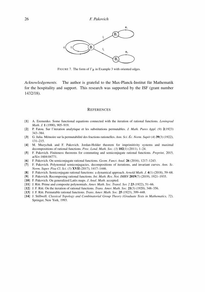
6.4. The group G B for B =−2z2/(z4+ 1). Since equality (25) implies that the
function
W =z2− 1
z2 + 1commutes with B, the group G B clearly contains a cyclic group of order two generatedby W . Moreover, it is easy to see that in fact G B = Z/2Z. Indeed, providing edges of thegraph 0B with orientations shown in Figure 7, we see that π1(0B, B) is a free group ofrank four with generators
c, t, l−1i ei li , i = 1, 2,
and assuming thatF(c)= F(e1)= F(e2)= z, F(t)=W,
we see that G B is generated by the W . Similarly, one can conclude that G B1 is generatedby X , where
X = F(l1tl−11 )=
z2+ 1z◦
z2− 1
z2 + 1◦ −
2z2 − 2
.
The above functions B1 and X provide an example of commuting rational functionssimilar to that constructed by Ritt. Namely, set
V =z2+ 1z
, U =−2
z2 − 2.
Then W commutes with U ◦ V =W ◦2, but W 6∈ CV . Indeed, assume the inverse, and letS be the rational function defined by any of the sides of the equality
z2+ 1z◦
z2− 1
z2 + 1= R ◦
z2+ 1z
, (42)
where R ∈ C(z). Then substituting z by 1/z in the right-hand side of (42), we obtain thatS ◦ 1/z = S. However, substituting z by 1/z in the left-hand side, we obtain
S ◦1z=
z2+ 1z◦ −
z2− 1
z2 + 1=−S.
The contradiction obtained shows that W 6∈ CV . Therefore, by Lemma 6.8, the rationalfunction
X = V ◦W ◦U
commutes with B1 = V ◦U , but is not a rational function in B1. Note that in distinctionwith the Ritt example, the non-triviality of G B1 is explained by the existence in the class[B1] of a function that is an iterate.
26 F. Pakovich
FIGURE 7. The form of 0B in Example 3 with oriented edges.
Acknowledgements. The author is grateful to the Max-Planck-Institut fur Mathematikfor the hospitality and support. This research was supported by the ISF (grant number1432/18).
REFERENCES
[1] A. Eremenko. Some functional equations connected with the iteration of rational functions. LeningradMath. J. 1 (1990), 905–919.
[2] P. Fatou. Sur l’iteration analytique et les substitutions permutables. J. Math. Pures Appl. (9) 2(1923)343–384.
[3] G. Julia. Memoire sur la permutabilite des fractions rationelles. Ann. Sci. Ec. Norm. Super (4) 39(3) (1922),131–215.
[4] M. Muzychuk and F. Pakovich. Jordan-Holder theorem for imprimitivity systems and maximaldecompositions of rational functions. Proc. Lond. Math. Soc. (3) 102(1) (2011), 1–24.
[5] F. Pakovich. Finiteness theorems for commuting and semiconjugate rational functions. Preprint, 2015,arXiv:1604:04771.
[6] F. Pakovich. On semiconjugate rational functions. Geom. Funct. Anal. 26 (2016), 1217–1243.[7] F. Pakovich. Polynomial semiconjugacies, decompositions of iterations, and invariant curves. Ann. Sc.
Norm. Super. Pisa Cl. Sci. (5) XVII (2017), 1417–1446.[8] F. Pakovich. Semiconjugate rational functions: a dynamical approach. Arnold Math. J. 4(1) (2018), 59–68.[9] F. Pakovich. Recomposing rational functions. Int. Math. Res. Not. IMRN 2019(7) (2019), 1921–1935.[10] F. Pakovich. On generalized Lates maps. J. Anal. Math. accepted.[11] J. Ritt. Prime and composite polynomials. Amer. Math. Soc. Transl. Ser. 2 23 (1922), 51–66.[12] J. F. Ritt. On the iteration of rational functions. Trans. Amer. Math. Soc. 21(3) (1920), 348–356.[13] J. F. Ritt. Permutable rational functions. Trans. Amer. Math. Soc. 25 (1923), 399–448.[14] J. Stillwell. Classical Topology and Combinatorial Group Theory (Graduate Texts in Mathematics, 72).
Springer, New York, 1993.