NIST Special Publication 1197

Community Resilience Economic Decision Guide for Buildings and

Infrastructure Systems

Stanley W. Gilbert David T. Butry

Jennifer F. Helgeson Robert E. Chapman

This publication is available free of charge from: http://dx.doi.org/10.6028/NIST.SP.1197

NIST Special Publication 1197

Community Resilience Economic Decision Guide for Buildings and

Infrastructure Systems

Stanley W. Gilbert David T. Butry

Jennifer F. Helgeson Robert E. Chapman

Applied Economics Office Engineering Laboratory

This publication is available free of charge from: http://dx.doi.org/10.6028/NIST.SP.1197

December 2015

U.S. Department of Commerce Penny Pritzker, Secretary

National Institute of Standards and Technology

Willie May, Under Secretary of Commerce for Standards and Technology and Director

Certain commercial entities, equipment, or materials may be identified in this document in order to describe an experimental procedure or concept adequately.

Such identification is not intended to imply recommendation or endorsement by the National Institute of Standards and Technology, nor is it intended to imply that the entities, materials, or equipment are necessarily the best available for the purpose.

National Institute of Standards and Technology Special Publication 1197 Natl. Inst. Stand. Technol. Spec. Publ. 1197, 69 pages (December 2015)

http://dx.doi.org/10.6028/NIST.SP.1197 CODEN: NSPUE2

ii

Abstract This Economic Guide provides a standard economic methodology for evaluating investment decisions aimed to improve the ability of communities to adapt to, withstand, and quickly recover from disruptive events. The Economic Guide is designed for use in conjunction with the NIST Community Resilience Planning Guide for Buildings and Infrastructure Systems, which provides a methodology for communities to develop long-term plans by engaging stakeholders, establishing performance goals for buildings and infrastructure systems, and developing an implementation strategy, by providing a mechanism to prioritize and determine the efficiency of resilience actions. The methodology described in this report frames the economic decision process by identifying and comparing the relevant present and future streams of costs and benefits—the latter realized through cost savings and damage loss avoidance—associated with new capital investment into resilience to those future streams generated by the status-quo. Topics related to non-market values and uncertainty are also explored. This report provides context for increasing resilience capacity through focusing on those investments that target key social goals and objectives, and providing selection criteria that ensure reduction of risks as well as increases in resilience. Furthermore, the methodological approach aims to enable the built environment to be utilized more efficiently in terms of loss reduction during recovery and to enable faster and more efficient recovery in the face of future disasters. Keywords Benefit-cost analysis; buildings; communities; constructed facilities; resilience; economic analysis; economic decision tool; life-cycle costing; natural and man-made hazards; present expected value; resilience; risk assessment; vulnerability

iii

iv

Preface Since 2002, the U.S. has endured seven of the 10 most costly disasters in its history, with Hurricane Katrina and Superstorm Sandy topping the list. There is a need for best practices for resilience planning that address the increasing value-at-risk of U.S. infrastructure and communities. Communities, as a system, are particularly vulnerable to the effects of natural and human-caused disruptive events. There are best practices for community resilience assessment methodologies; however, there are gaps that remain in characterization of robust, benefit-cost measures of community resilience, especially in the planning process. In many cases, resilience remains in a planning silo and is considered separately by communities from economic growth or disaster risk planning. Efforts to increase resilience capacities are best realized when resilience is considered as an attribute in general community planning efforts, especially in planning and implementing building and infrastructure projects. Despite significant progress in the application of science and technology to disaster reduction, communities are still challenged by disaster preparation, response, and recovery. Although the number of lives lost each year to natural and human-caused disasters is trending downward, the costs following major disasters continue to rise in part due to the increasing amount of at-risk infrastructure. Reliance on rebuild-as-before strategies is impractical and inefficient when dealing with persistent hazards. Instead, communities must break the cycle by enhancing their resilience with a systemic view of short- and long-run time horizons. High-priority science and technology investments, coupled with sound decision-making at all levels (national, regional, and local), will enhance community resilience and thus reduce vulnerability. The National Institute of Standards and Technology (NIST) develops unbiased, state-of-the-art measurement science that advances the Nation’s technology infrastructure and is needed by industry to continually improve products and services. The mission of NIST’s Engineering Laboratory is to promote U.S. innovation and industrial competitiveness in areas of critical national priority by anticipating and meeting the measurement science and standards needs for technology-intensive manufacturing, construction, and cyber-physical systems in ways that enhance economic prosperity and improve the quality of life. Community resilience is a recognized critical national priority—one that requires meaningful and rigorous measurement science for establishing suitable performance metrics and planning tools. To address this need, NIST launched an effort to develop, organize, and convene a work program to help develop new and innovative approaches to community resilience and the underlying decision-making processes. This multi-faceted program (NIST Community Resilience Program) is aimed towards development of tools for resilience planning that assist communities and related stakeholders whose work and interests relate to the buildings and physical infrastructure systems of those communities. Guidance on economic decision-making specific to resilience is a key part of this effort, as it aids communities in better understanding the benefits, costs, and tradeoffs involved in making capital improvements (changes) to the built environment for increased resilience. The guidance in this report is intended to assist users of the NIST Community Resilience Planning Guide for Buildings and Infrastructure Systems by recognizing the key roles buildings and infrastructure system play in supporting the social and economic functions of communities.

v

vi

Acknowledgements The authors wish to thank all those who contributed ideas and suggestions for this report, including participants at the NIST-ASCE-ASME Workshop on the Economics of Community Disaster Resilience that was held April 29-30, 2015 in Reston, VA. Special appreciation is extended to Bilal Ayyub, University of Maryland; Stephen Cauffman, NIST; Harvey Cutler, Colorado State University; Mark Ehlen, Sandia National Laboratories; Howard Harary, NIST; George Huff, The Continuity Project; Muthiah Kasi, Alfred Benesch & Company; Erica Kuligowski, NIST; Nicos Martys, NIST; Therese McAllister, NIST; Nancy McNabb, NIST; Adam Rose, University of Southern California; Martin Shields, Colorado State University; Douglas Thomas, NIST; Sammy Zahran, Colorado State University. Author Information Stanley W. Gilbert Economist Applied Economics Office Engineering Laboratory National Institute of Standards and Technology 100 Bureau Drive, Mailstop 8603 Gaithersburg, MD 20899-8603 Tel.: 301-975-5261 Email: stanley.gilbert@nist.gov David T. Butry Economist Applied Economics Office Engineering Laboratory National Institute of Standards and Technology 100 Bureau Drive, Mailstop 8603 Gaithersburg, MD 20899-8603 Tel.: 301-975-6136 Email: david.butry@nist.gov Jennifer F. Helgeson Economist Applied Economics Office Engineering Laboratory National Institute of Standards and Technology 100 Bureau Drive, Mailstop 8603 Gaithersburg, MD 20899-8603 Tel.: 301-975-6133 Email: jennifer.helgeson@nist.gov Robert E. Chapman Chief, Applied Economics Office National Institute of Standards and Technology Engineering Laboratory 100 Bureau Drive, Mailstop 8603 Gaithersburg, MD 20899-8603

vii

Tel.: 301-975-2723 Email: robert.chapman@nist.gov Disclaimers The policy of the National Institute of Standards and Technology is to use metric units in all of its published materials. Because this report is intended for an audience that often uses U.S. customary units, it is more practical and less confusing to include U.S. customary units as well as metric units. Measurement values in this report are therefore stated in metric units first, followed by the corresponding values in U.S. customary units within parentheses. Cover Photographs All photographs used are public domain images under Creative Commons CC0.

viii

Table of Contents

Abstract ...................................................................................................................................................... ii Preface ....................................................................................................................................................... iv

Acknowledgements .................................................................................................................................. vi 1 Introduction ....................................................................................................................................... 1

1.1 Purpose ...................................................................................................................................... 1

1.2 Approach ................................................................................................................................... 1

2 NIST Community Resilience Program ............................................................................................ 3

2.1 NIST Community Resilience Planning Guide for Buildings and Infrastructure Systems ........ 3

2.2 NIST Community Resilience Implementation Guidelines and the Community Resilience Panel 4

2.3 Disaster Resilience Fellows ...................................................................................................... 4

2.4 Community Resilience Center of Excellence ........................................................................... 5

2.5 NIST’s Applied Economics Office (AEO) Research ............................................................... 5

3 Community Resilience ....................................................................................................................... 7

3.1 Defining Resilience ................................................................................................................... 7

3.2 The Disaster Cycle and Role of Intervention ............................................................................ 8

3.3 Measuring Resilience .............................................................................................................. 10

3.4 Planning for Resilience ........................................................................................................... 12

3.5 Resilience Dividend: Making the Business Case for Resilience ............................................ 13

4 Economic Decision Guidelines ........................................................................................................ 15

4.1 Select Candidate Strategies ..................................................................................................... 17

4.1.1 Form a Collaborative Planning Team ................................................................................. 17

4.1.2 Understand the Situation ..................................................................................................... 17

4.1.3 Determine Community Goals and Objectives .................................................................... 17

4.1.4 Plan Development ............................................................................................................... 18

4.2 Define Investment Objectives and Scope ............................................................................... 18

4.2.1 Define Economic Objective Function ................................................................................. 18

4.2.2 Determine Planning Horizon .............................................................................................. 18

4.2.3 Identify Constraints ............................................................................................................. 19

4.3 Identify Benefits and Costs ..................................................................................................... 19

4.3.1 Identify Costs and Losses ................................................................................................... 20

4.3.2 Identify Benefits and Savings ............................................................................................. 20

4.3.2.1 Reductions in Disaster Costs and Losses .........................................................20

ix

4.3.2.2 Non-Disaster-Related Benefits .........................................................................21 4.3.3 Identify Externalities ........................................................................................................... 22

4.4 Identify Non-Market (Non-Economic) Considerations .......................................................... 22

4.5 Define Analysis Parameters .................................................................................................... 23

4.5.1 Select Discount Rate ........................................................................................................... 23

4.5.2 Define Probability Distributions ......................................................................................... 24

4.5.3 Define Risk Preference ....................................................................................................... 25

4.6 Perform Economic Evaluation ................................................................................................ 26

4.6.1 Compute Present Expected Value ....................................................................................... 26

4.6.1.1 Alternative Formulations ..................................................................................26 4.6.2 Evaluate Impact of Uncertainty .......................................................................................... 27

4.7 Rank Strategies ....................................................................................................................... 28

4.7.1 Plan Preparation, Review, and Approval ............................................................................ 29

4.7.2 Plan Implementation and Maintenance ............................................................................... 29

5 Future Directions ............................................................................................................................. 31

References ................................................................................................................................................ 33

Appendix A: Community Resilience Economic Decision Example – Riverbend, USA .................... 37

Appendix B: Exposition of Model ......................................................................................................... 43

Appendix C: Technique for Loss Estimation ....................................................................................... 47

x

List of Figures Figure 1: Disaster Cycle. Based on Rubin (1991)....................................................................................... 9 Figure 2: Flow chart illustrating elements and connections within the Economic Guide, and highlighted linkages with the Planning Guide. ............................................................................................................ 16

xi

List of Tables Table 4-1: Estimated direct and indirect damages for selected disasters. ................................................. 21 Table A-1: Inputs to the Economic Evaluation......................................................................................... 40 Table A-2: Outputs of the Economic Evaluation. ..................................................................................... 41

xii

List of Acronyms AEO Applied Economics Office

ASTM American Society for Testing and Materials

BRIC Baseline Resilience Indicators for Communities

CARRI CRS Community and Regional Resilience Institute’s Community Resilience System

CART Communities Advancing Resilience Toolkit

CGE Computable General Equilibrium

CoE Center of Excellence

CRF Community Resilience Framework

CRP Community Resilience Panel

DHS Department of Homeland Security

DOT Department of Transportation

DRF Disaster Resilience Fellows

DSER Direct Static Economic Resilience

EL Engineering Laboratory

EOP Executive Office of the President

FEMA Federal Emergency Management Agency

FHWA Federal Highway Administration

GDP Gross Domestic Product

IPCC Intergovernmental Panel on Climate Change

NIST National Institute of Standards and Technology

PPD Presidential Policy Directive

SDR Subcommittee on Disaster Reduction

TSER Total Static Economic Resilience

USC United States Codes

xiii

1

1 Introduction This publication (‘Economic Guide’) develops economic decision guidance for evaluation of alternate investments designed to improve community resilience through strengthening the ability to respond, withstand, and recover from disruptive events. It is designed to implement the principles and attributes of resilient communities upon which enhanced resilience may be developed, evaluated, and implemented. A common attribute of resilient communities is risk management through an integrated approach to managing threats and opportunities for decision-making that is balanced and informed. Developed by the Applied Economics Office (AEO) at the National Institute of Standards and Technology (NIST), this guidance will assist users of the NIST Community Resilience Planning Guide for Buildings and Infrastructure Systems (‘Planning Guide’) in understanding the benefits, costs, and tradeoffs involved in making capital improvements to the built environment for increased resilience, recognizing the key roles buildings and infrastructure systems play in supporting the social functions of a community. The guidance follows industry-standard economic methods, ensuring that different analyses of alternative infrastructure investments can be compared with each other and to a business-as-usual baseline. 1.1 Purpose Communities in the United States experience natural, technological and human-caused hazards every year. When a hazard severely disrupts a community’s ability to function, it becomes a disaster. Severe storms, hurricanes, storm surge, tornados, wildfires, earthquakes, snow and ice, and human-caused disruptions lead to numerous Presidential disaster declarations and billions of dollars in losses every year (Swiss Re, 2014). There is an abundance of research focused on topics related to community resilience, including best-practices for community assessment; however, guidance is needed to evaluate the economic ramifications of investment decisions into capital infrastructure for the purpose of improving community resilience. The purpose of this report is to provide a standard economic methodology for evaluating investment decisions aimed to improve the ability of communities to adapt to, withstand, and quickly recover from disasters. The Economic Guide frames the economic decision process by identifying and comparing the relevant present and future streams of costs and benefits to a community—the latter realized through cost savings and damage loss avoidance—associated with new capital investment into resilience to those generated by the status-quo. This report provides a means to increase the capacity of communities to objectively and effectively compare and contrast capital investment projects through consideration of benefits and costs while maintaining an awareness of system resilience. Topics related to non-market values and uncertainty are also explored. 1.2 Approach The guidelines in this report are designed for use in conjunction with the Planning Guide by providing a mechanism to prioritize and determine, based on supporting community social needs, the efficiency of resilience actions. The Planning Guide provides a methodology for communities to develop long-term plans by engaging stakeholders, establishing performance goals for buildings and infrastructure systems, and developing an implementation strategy.

2

This Economic Guide supports community resilience through focusing on those investments that target key social goals and objectives, and providing selection criteria that ensure reduction of risks as well as increases in resilience. Furthermore, the methodological approach enables decision making for the built environment in terms of loss reduction and faster and more efficient recovery in the face of future hazard events. The Economic Guide contains three chapters and three appendices in addition to the Introduction. Chapter 2 provides an overview of the NIST effort into community resilience. Chapter 3 introduces concepts related to community resilience, focusing on measurement and planning. Chapter 4 details the economic decision guidelines. It outlines a process for considering alternate methods for increasing community resilience through cost-effective investments in the built environment and other infrastructure. These guidelines are targeted to address the need for characterization of and decisions between robust, benefit-cost measures of community resilience, especially in the planning process. Appendix A provides an example that illustrates use/application of the process described in the Economic Guide. The guidelines described in Chapter 4 are followed through using an illustrative example. Appendix B contains a mathematical description of the benefit/cost model under the Economic Guide model. It describes it in two forms: 1. maximizing net benefits and 2. minimizing cost plus loss, and compares the two. Appendix C describes select techniques for estimating the economic costs of losses that occur from natural and human-caused disasters.

3

2 NIST Community Resilience Program Community resilience is a recognized critical national priority—one that requires meaningful and rigorous measurement science for establishing suitable performance metrics and planning tools. To address this need, NIST launched an effort to develop new and innovative approaches to community resilience and the underlying decision-making processes. The multi-faceted NIST Community Resilience Program is developing of tools for resilience planning that assist communities and related stakeholders whose work and interests relate to the buildings and physical infrastructure systems of those communities. The guidance in the Economic Guide is intended to assist users of the NIST Planning Guide with economic decision-making specific to resilience is a key part of this effort, as it aids communities in better understanding the benefits, costs, and tradeoffs involved in making capital improvements (changes) to the built environment for increased resilience. There are a number of significant areas covered by NIST’s Community Resilience program efforts. The programmatic structure is interdisciplinary, such that resilience is considered as a dynamic system property in the engineering and structural planning for buildings and infrastructure as well as the economic (development) planning and assessments of related social aspects. The approaches that are taken under the NIST Community Resilience program are outlined, below. 2.1 NIST Community Resilience Planning Guide for Buildings and Infrastructure

Systems The Planning Guide (NIST 2015a; NIST 2015b) provides a methodology for local government to bring together all of the relevant stakeholders to establish performance goals to maintain the social and economic fabric when disruptive events occur; in other words, to be resilient. The Planning Guide is intended to support long-term community planning. The methodology is focused on the role that buildings and infrastructure play in assuring that social and economic functions are able to resume in a manner that does not result in detrimental impacts after a disruptive event. When catastrophic events occur, the community will have plans in place to rebuild in a thoughtful way to be better prepared for future events, including coordination with state and federal agencies as outlined in the National Preparedness Goal. The Planning Guide supports the National Preparedness Goal by providing planning guidance at the local level to support achieving the outcome of community resilience. Per the Planning Guide (NIST 2015a, pgs. 3-4):

A six-step methodology is described that helps communities develop customized resilience plans by bringing together all relevant stakeholders, establishing community-level performance goals, and developing and implementing plans to become resilient. This approach focuses on the roles that buildings and physical infrastructure systems – the built environment – play in assuring social functions resume when needed after a hazard event. Those functions include government, business, healthcare, education, community services, religion, culture, and media communications. If a catastrophic event does occur, resilience planning encourages and enables the community to have plans in place to rebuild in a thoughtful way. That includes coordination with nearby communities as well as with state, regional, and federal agencies.

4

The [Planning] Guide can help a community to:

• Build on, broaden, bridge, and integrate its current plans (e.g., economic, emergency preparedness, land use) with community resilience plans, particularly for the built environment.

• Better define risks, priorities, and pre- and post-event costs, including the consequences of not taking certain actions.

• Prioritize resilience actions for buildings and infrastructure systems, based on the specific hazards a community is most likely to face and the importance of these buildings and infrastructure systems in supporting key social functions.

Communities striving to prepare for and deal with disasters can be overwhelmed by a host of issues, policies, and regulations to address. Each demands time and investment to resolve. Experience shows that communities generally over-estimate their ability to successfully deal with hazard events, as evidenced by the number of Presidential Disaster Declarations each year (FEMA, 2011). It may also be that communities either underestimate risk exposure or assume that meaningful improvements are cost-prohibitive. Transformative planning for resilience is often assigned a low priority unless a recent event focuses community interests. Even then, communities tend to focus on near-term restoration to previous conditions. 2.2 NIST Community Resilience Implementation Guidelines and the Community

Resilience Panel The future Community Resilience Implementation Guidelines are intended to promote best practices to help communities develop their own resilience plan. Given the broad scope of resilience, the Community Resilience Implementation Guidelines will provide guidance based on existing standards, codes, and best practices to assist communities in implementing their plans. The Community Resilience Panel (CRP) is planned to be a resource to support communities in their efforts to develop guidelines, best practices, and other tools for community resilience over time. There will be broad stakeholder input in the CRP for various topic area related to resilience; including: building construction and safety, business and industry, communications systems, community planning, community social institutions, education and research, energy systems, facility operations and maintenance, federal, tribal, regional, state, and local governments, insurance/re-insurance, public health and healthcare, relief services, standards development organizations, transportation systems, vulnerable populations, water/wastewater systems. The CRP is expected to consist of several hundred members working on multiple committees to address gaps in existing standards and develop products to inform efforts to enhance community resilience. 2.3 Disaster Resilience Fellows NIST has engaged Disaster Resilience Fellows (DRF) with specialized expertise working with communities, social science, recovery planning, business continuity, buildings, and physical infrastructure systems. DRFs are nationally recognized leaders in their field of expertise and bring a breadth and depth of knowledge and experience to advance the efforts of the Community Resilience program. These experts contribute to the development of the Planning Guide, activities of the CRP, and the Community Resilience Implementation Guidelines. Their exceptional expertise is in areas critical to community resilience and preparedness.

5

2.4 Community Resilience Center of Excellence The Community Resilience Center of Excellence (CoE) was established by NIST in February 2015 and is developing the science-basis for tools to support community resilience, including the development of integrated, systems-based computation models to assess community resilience and to guide community-level resilience investment decisions. The CoE, which is led by Colorado State University partnering with nine other universities, also will develop a data management infrastructure, as well as tools and best practices to improve the collection of disaster and resilience data. The economic research team under the CoE is addressing Economic Networks and Cascading Effects related to community resilience; this research is complementary to the NIST-led resilience economics efforts from the Applied Economics Office (AEO) within the Engineering Laboratory (EL) at NIST. The CoE team plans to use two complementary economic impact modeling strategies to estimate direct and multiplier effects of assorted disruptive shocks in the economy: (1) applied econometric analyses of household and regional data to determine relationships between shocks and economic outcomes; and (2) computable general equilibrium (CGE) analyses to understand how hazard losses manifest in the local economy through industry-specific losses to critical infrastructure. 2.5 NIST’s Applied Economics Office (AEO) Research NIST’s AEO is engaged in efforts to develop greater understanding of the economic implications of resilience planning against natural and human-made disasters. The Economic Guide provides results of research conducted by the AEO concerning the valuation of community investment projects that consider resilience. The Economic Guide develops economic decision guidance for evaluation of alternate investments designed to improve community resilience through strengthening the ability to response, to withstand, and recover from disasters. It facilitates decision making designed to implement the principles and attributes of resilient communities upon which enhanced resilience may be developed, evaluated, and implemented. In 2015 NIST launched an effort to develop, organize, and convene a workshop on the economics of community resilience to guide NIST in developing a portfolio of programs that are focused on providing the enabling measurement science to key industry stakeholders. NIST led the workshop that included more than 70 participants, representing a wide variety of stakeholders, including academia, community planners, government executives, policy makers, and subject matter experts in economics, engineering, finance, and risk analysis. The workshop was organized around three cross-cutting themes: (1) resilience planning and deployment; (2) dealing with uncertainty; and (3) economics of recovery. The outcomes of this workshop are reported in the NIST Special Publication: Economics of Community Disaster Resilience Workshop Proceedings (Ayyub et al. 2015).

6

7

3 Community Resilience Since 2002, the U.S. has endured seven of the 10 most costly disasters in its history, with Hurricane Katrina and Superstorm Sandy topping the list. In the past decade, average economic losses from extreme weather equated to about USD 190 billion per year and average insured losses were recorded to be about USD 60 billion per year (Swiss Re, 2014). As disaster losses to buildings and infrastructure are increasing exponentially, the trend is economically unsustainable (e.g. White et al., 2001). This section provides a brief overview of the meaning of resilience, the disaster cycle, ways to measure resilience, planning, and making the business case for resilience. For a comprehensive review of the literature on resilience, hazard assessment, vulnerability assessment, risk assessment, risk management, and loss estimation, see NIST Special Publication 1117, Disaster Resilience: A Guide to the Literature1. 3.1 Defining Resilience The concept of resilience as a systems property appears in different disciplines. It was formally introduced in ecology, defined as the persistence of relationships within a system (Holling, 1973) – it is measured by the system’s ability to absorb change-state variables, driving variables and parameters and still persist. Gilbert (2010) notes that in general, definitions of resilience fall into two broad categories: (1) outcome-oriented and (2) process-oriented. An outcome-oriented definition defines resilience in terms relative to an end result—e.g., time to recovery. A process-oriented definition defines resilience as a progression towards a desired outcome—e.g., ability to adapt. Presidential Policy Directive 8 (PPD-8 2011) defines resilience as “the ability to adapt to changing conditions and withstand and rapidly recover from disruption due to emergencies.” PPD-21 (2013) on Critical Infrastructure Security and Resilience expanded the definition to include “the ability to prepare for and adapt to changing conditions and to withstand and recover rapidly from disruptions. Resilience includes the ability to withstand and recover from deliberate attacks, accidents, or naturally occurring threats or incidents.” The term disaster refers to “a serious disruption of the functioning of a community or a society causing widespread human, material, economic or environmental losses which exceed the ability of the affected community or society to cope using its own resources”2. The National Research Council (2012) defined resilience as the ability to prepare and plan for, absorb, recover from or more successfully adapt to actual or potential adverse events as a consistent definition with U. S. governmental agency definitions (SDR 2005, DHS 2008 and PPD-8 2011). In this Economic Guide, economic recovery includes the preparation for repair and reconstruction ex-post a disaster event. It should be noted that community recovery can take place without full repair and recovery (Rose, 2009). Rose & Krausmann (2013) differentiate between static and dynamic economic resilience. Static economic resilience is the “efficient use of remaining resources at a given point in time” (Rose, 2015). Dynamic economic resilience is the “efficient use of resources over time for investment in repair and reconstruction” (ibid.). This type of resilience describes the ability and speed of recovery efforts through sound investment in repair and reconstruction that may require time trade-offs; for example, recovery efforts may require temporary use of older infrastructure to house emergency services (Baird, 2010) or to allow for reduced business interruption (e.g. Rose, 2009). 1 Gilbert, 2010. <http://www.nist.gov/manuscript-publication-search.cfm?pub_id=906887> 2 National Science and Technology Council, 2005.

8

3.2 The Disaster Cycle and Role of Intervention Ahead of a potential disaster event, capital investments in infrastructure should be made that are expected to perform well both under business-as-usual as well as during the recovery period. Resilience is complicated by the deep uncertainty surrounding covariate shocks3 (e.g. IPCC, 2012). The relative uncertainties in timing of onset, the magnitude of the event, as well as the potential for cascading risks challenge implementation of current economic valuation techniques in planning, especially for the built environment. The stages in the disaster cycle (e.g. Rubin, 1991) (Figure 1) can be considered to fall into two groups: (1) response and recovery and (2) mitigation and prevention/protection (Gilbert, 2010). Traditionally, mitigation and prevention/protection typically occur well ahead of the realization of the natural and human-made disaster and are aimed specifically at making a given system more resilient towards a given hazard. Response and recovery tend to take place in the period immediately following a disaster. An issue with this conceptualization is the acceptance disasters will occur, and repeatedly. While to the extent possible, community planning for resilience should consider pathways that address mitigation, prevention/protection, response, and recovery, the goal of effective planning should be to break the cycle—shocks become disruptive, but manageable, events instead of disasters. Another important distinction is between inherent and adaptive resilience. Inherent resilience refers to elements of resilience that have been already built into the system, such as available inventories, substitutable inputs, and contractual arrangements for imports from outside the affected area (Rose, 2015). Resilience capacity can be built up through these means and is then accessed after the disaster. Adaptive resilience arises out of improvisation under stress, such as draconian conservation otherwise not thought possible (e.g., working many weeks without heat or air conditioning), changes in the way goods and services are produced, and new contracting arrangements that match customers who have lost their suppliers with suppliers who have lost their customers.

3 Covariate shocks, as opposed to idiosyncratic shocks, describe highly correlated risks across space, e.g. the weather risks that affect many members of a community simultaneously, which can be difficult to insure due to nature of occurrence and the magnitude of impact.

9

Figure 1: Disaster Cycle. Based on Rubin (1991)

Experience with disruptive events can be used to help refine resilience planning, increasing its efficiency and effectiveness. Integrated risk management is a “continuous, proactive, and systemic process that is structured through ongoing learning and evaluation” (e.g. Radermacher et al., 2010) and can be undertaken at different levels of analysis. This view of risk management identifies a series of target-oriented efforts to manage the potential (adverse) consequences of disaster events, which may otherwise prevent a community from achieving its medium- and long-term potentials. In the analysis of resilience, there is a need to consider systemic dynamics within a cyclical process characterized by time periods ex-ante and ex-post realization of the disaster event. Ex-ante consideration often involve mitigation activities which reduce and transfer risks to the socio-economically efficient levels. Ex-post considerations often involve adaptation of planned resilience activities in order to conform to the reality of outcomes from the disaster event. In some cases there are residual effects to the infrastructure system that result in (short-term) unrecoverable losses. To the extent possible these possibilities should be considered in communities’ selection of alternative scenarios to be considered for resilience planning. In studies of the effect of hazard events, there is rarely consensus surrounding the distribution of exposure, vulnerability or possible outcomes (Kunreuther et al., 2013). Generally agreed-upon probability distributions are not always available for hazard effects, especially those related to social impacts, and stakeholders differ in their degree of risk tolerance .4 This uncertainty is more ambiguous 4 Worst-case scenarios -- the possibility of extremely costly outcomes with small, but positive probabilities – can have large impacts on evaluations by benefit-cost analysis related to resilience. These low-probability high-consequence events have motivated a focus on the tail of the distribution of outcomes. For example, a small chance of a truly unacceptable outcome may have a significant impact when evaluating the expected benefits and costs.

Normal (Status Quo)

Mitigation

Prevention & Protection

Disaster (Event)

Response

Recovery

10

in consideration of effects on systems within a community due to dependencies between system components. Policy analyses through the use of standard approaches, such as expected utility theory and benefit-cost analysis have been adapted to address this issue. This perspective highlights the value of robust decision-making tools designed for situations such as evaluating climate policies, where consensus on probability distributions is not available and stakeholders differ in their degree of risk tolerance. Many of the uncertainties in potential outcomes of resilience efforts are temporal in nature. It is not always clear when benefits of mitigation activities will accrue. Quantifying the probability that benefits will be realized for a particular mitigation strategy is a first step in addressing such uncertainties within a benefit-cost framework. Temporal uncertainties generally arise from uncertainties in the interaction between outcomes of current resilience efforts and future hazard events. Uncertainty may include frequency and intensities of future hazards as well as future resources, including human, social, produced, natural and financial resources that will be available to address mitigation to these future hazard events. To this point, current best practice generally assumes that the statistics and models based on past frequencies and intensities will apply to future hazards. Observations of climate and weather patterns as well as changes in human behavior indicate temporal uncertainties exist. Temporal uncertainties also apply to the characteristics assumed of the amount of human, social, produced, natural and financial resources available in the future. 3.3 Measuring Resilience There is a need for best practices for resilience planning that address the amount of at-risk infrastructure in the United States. At present, most existing approaches do not explicitly take into account economic valuation measurements. Communities, as a system, are particularly vulnerable to the effects of natural and human-caused disruptive events. Proposed resilience metrics and indicators range in their use of descriptive, quantitative or mixed methodologies; whether they are based on interview, expert opinions, engineering analysis or employ pre-existing datasets (NIST, 2015b). Regardless of assessment methodology and presentation of the resilience “score” (i.e. overall score or separately reported scores across factors or sectors), these metrics and indicators strive to address: (1) how community leaders know the level of resilience of the community and (2) provide a background against which to assess if changes implemented to improve community resilience are making a significant difference (National Academies, 2012). Select examples of these metrics and indicators are noted below. PEOPLES’ Framework MCEER (Renschler et al., 2010) developed a framework for measuring resilience. There are seven elements in the framework (represented by the acronym ‘PEOPLES’), which explicitly includes a metric for effects on economic development. The seven elements are as follows:

1. Population and Demographics 2. Environmental/Ecosystem 3. Organized Governmental Services 4. Physical Infrastructure 5. Lifestyle and Community Competence 6. Economic Development 7. Social-Cultural Capital

The majority of elements are self-explanatory. Protecting people means, among other things, preventing deaths and injuries and preventing people from being made homeless. Protecting physical infrastructure

11

means limiting damage to buildings and structures, including most lifeline infrastructure. Protecting the economy means preventing job losses and business failures, and preventing business interruption losses. Protecting key government services includes (among other things) ensuring that emergency services are still functioning. Protecting social networks and systems includes (among many other things) ensuring that people are not separated from friends and family (Gilbert, 2010). Baseline Resilience Indicators for Communities The Baseline Resilience Indicators for Communities (BRIC) (Cutter et al., 2014) process is based on empirical research with conceptual and theoretical underpinnings. The BRIC measures overall pre-existing community resilience, which can help communities develop a baseline measure of resilience that can be used in a policy context (NIST, 2015b). Using data from 30 public and freely available sources, BRIC comprises 49 indicators associated with six domains:

• Social (10 indicators) • Economic ( 8 indicators) • Housing and Infrastructure (9 indicators) • Institutional (10 indicators) • Community Capital (7 indicators) • Environmental (5 indicators)

Indicators in these domains determine areas that policy- and decision makers should invest for planning intervention strategies to create more robust community resilience. City Resilience Framework Another tool is the City Resilience Framework (CRF), a framework “for articulating city resilience” developed by Arup (2014) with support from the Rockefeller Foundation 100 Resilient Cities initiative. This framework organizes 12 identified “key indicators” into four categories:

• Leadership and strategy • Health and wellbeing • Infrastructure and environment • Economy and social

The 12 key indicators span seven qualities of what is considered a resilient city under this framework: being reflective, resourceful, robust, inclusive, redundant, integrated, and/or flexible. The CRF integrates social, economic and physical aspects of resilience and it considers human-driven processes as inherent components of the system-of-systems that defines a community. Community and Regional Resilience Institute’s Community Resilience System In some cases, base practices for resilience assessments involve working with community stakeholders in a process-oriented methodology. For example, the Community and Regional Resilience Institute’s Community Resilience System (CARRI CRS, 2013) “is an action-oriented, web-enabled process that helps communities to assess, measure, and improve their resilience to … threats and disruptions of all kinds, and ultimately be rewarded for their efforts.” The Community Resilience System (CRS) includes both a pre-existing knowledge base to help inform communities on their resilience path and a process guide that provides a systematic approach to moving from expressed interest in improved resilience to the visioning and action planning steps (NIST, 2015b).

12

Communities Advancing Resilience Toolkit The Communities Advancing Resilience Toolkit (CART) (TDC, 2012) was developed by the Terrorism and Disaster Center at the University of Oklahoma Health Sciences Center.5 The CART approach is not hazard specific, and it is applicable across communities of varying size and type as a means of enhancing community resilience through planning and action. It engages community organizations in collecting and using assessment data to develop and implement solutions for building community resilience for disaster prevention, preparedness, response, and recovery. The CART process uses a combination of qualitative and quantitative approaches and provides a complete set of tools and guidelines for communities to assess their resilience across a number of domains (NIST, 2015b). Resilience Index for Business Recovery Rose (2009) offers an overview of definitions for resilience from different disciplines and notes that there are some importance distinctions of those focused on economic resilience of a community. For example, it is noted that economic approaches often focus on the flows of goods and services that are direct measures of economic well-being (e.g., GDP and employment). This index offers a framework for choosing short-run indicators of economic resilience based on economic production theory and extends to resilience of the operation of businesses (Rose, 2009). In this framework Direct Static Economic Resilience (DSER) refers to the level of the individual firm or industry and looks at the operation of an individual business or household entity. DSER is “the percentage of the maximum economic disruption that a particular shock could bring about” (Rose and Krausman, 2013). The Total Static Economic Resilience (TSER) refers to the economy as a whole as a set of integrated supply chains and “includes all of the price and quantity interactions in the economy” (ibid.). The framework presents static and dynamic resilience strategies for businesses on the customer and supplier sides. In turn, each resilience activity is applicable to one or more inputs (e.g., labor, infrastructure, materials) or outputs of economic activity (Rose, 2009). On the supplier side examples of dynamic resilience strategies include: removing operating impediments and improved management effectiveness. Static resilience strategies that mute losses at the microeconomic-level include: conservation, input substitution, and emergency stockpiles in inventories (Rose and Krausman, 2013). Similar structures for government and households are noted in Rose (2009). A recognized goal of constructing a resilience index is to study the recovery process after a hazard event, but also to allow for improvements to the process. Rose (2007) presents a time path of a sequencing of steps related to dynamic and static resilience in the economic system. There are additional metrics and indicators for measuring aspects of community resilience,6 see Chapter 16 (Community Resilience Metrics) of the Planning Guide (NIST, 2015b); however, there are gaps that remain in characterization of robust, benefit-cost effective measures of community resilience that provide distinct guidance on the selection among potential resilience-based alternative investments, which this Economic Guide seeks to address. 3.4 Planning for Resilience The NIST Planning Guide details a six-step process for community leaders to develop and implement a resilience plan (NIST, 2015a). It creates a proactive process to ensure critical social functions of the community are supported during and after a disruptive event occurs. The six steps are briefly described below. 5 It was funded by the Substance Abuse and Mental Health Services Administration, U.S. Department of Health and Human Services, and the National Consortium for the Study of Terrorism and Responses to Terrorism, U.S. Department of Homeland Security, and by the Centers for Disease Control and Prevention. 6 THRIVE, Coastal Community Resilience Index, PEOPLES Framework, ResilUS.

13

1. Form a Collaborative Planning Team The objective is to identify the resilience leader(s) and critical team members, and engage with key public and private stakeholders for input into the planning and implementation stages.

2. Understand the Situation The objective is to characterize the social dimensions and built environment, by developing an understanding of the social functions that buildings and infrastructure system support. The social institutions includes: family, health, economy, education, government, religious and cultural beliefs, community service, and the media. The built environment includes: buildings, energy, transportation, communication, and water and wastewater sectors.

3. Determine Community Goals and Objectives The objective is to establish long term community goals based on desired recovery performance goals for the built environment. It includes defining community hazards and the current expected performance of systems during and after hazard events in their ability to support social functions.

4. Plan Development The objective is to perform gap analysis between the current and desired performance goals, and to identify and prioritize potential solutions as a basis for the implementation strategy.

5. Plan Preparation, Review, and Approval The objective is to document the resilience plan, and implementation strategies, and obtain approval from the community of stakeholders.

6. Plan Implementation and Maintenance The objective is to execute the plan, and to revisit it on a periodic basis.

The way in which the six-step process outlined in the NIST Planning Guide fits hand-in-glove into the Economic Guide methodology is illustrated in Figure 2. NIST Planning Guide steps 1 through 4 are listed under the heading of Select Candidate Strategies in Figure 2. NIST Planning Guide steps 5 and 6 are listed under the heading of Rank Strategies in Figure 2. It is important to note that the Economic Guide has step 4, Plan Development, as its primary focus. NIST Planning Guide steps 1 through 3 are used to identify the potential solutions referred to in step 4. The Economic Guide uses economic analysis techniques to prioritize the potential solutions, which is a key component of step 4. The analysis reports produced under the heading Perform Economic Evaluation provide the economic foundation for NIST Planning Guide steps 5 and 6. Figure 2 is explained in greater detail in Chapter 4. 3.5 Resilience Dividend: Making the Business Case for Resilience Uncertainty surrounding occurrence frequency, magnitude, and timing of a disaster can make a benefit-cost analysis of resilience measures difficult when a community may prefer to spend a limited budget on capital investments expected to produce certain outcomes in the business-as-usual case. There is a growing understanding that building resilience on a community-scale creates benefits in two dimensions: (1) enabling individuals, communities, and organizations to better withstand and recover from a disruption more effectively and (2) enables improvement to current systems (i.e. business-as-usual/status quo situation) (Rodin, 2014), by lessening the impact of chronic stresses (e.g., crime,

14

poverty, unemployment), thereby improving a community’s ability to maintain essential functions (Ayyub et al., 2015). This “resilience dividend” has been noted in a number of (qualitative) community and city case studies under which investment in financing and resources for future resilience yields current direct economic benefits (e.g. increased jobs) (ibid.). Methods for further implementing elements of the “resilience dividend” into upfront benefit-cost assessments of capital investments for resilience projects would likely improve the case for mainstreaming of resilience and help create less vulnerable communities.

15

4 Economic Decision Guidelines The time to plan for hazards is not after it strikes; however, the uncertainty surrounding the probabilities and consequences of potential hazards, cascading effects, and limited budgets can challenge planning efforts. Communities need an approach that helps them decide between alternatives that reduce damage levels and speed recovery with their limited economic resources. Ideally, resilience planning for physical infrastructure and related services will be woven into communities’ social and economic (growth) plans/systems in a way that supports community resilience. Shifting thinking towards recognizing the design and operation of buildings and infrastructure in communities into an interconnected system of systems, creates challenges for valuation and development of metrics for resilience. The standard benefit-cost analysis approach is challenged by attributes of resilience planning. Some of these key challenges and areas for future research related to economic decision making for resilience planning are noted in this section. The Economic Guide provides a process for considering alternate methods for increasing community resilience through cost-effective investments in the built environment and other infrastructure systems. It includes a step-wise methodology (Figure 2) for analyzing the economics of competing capital improvements and ultimately selecting economic investment strategies. The steps in the process are:

1. Select Candidate Strategies; 2. Define Investment Objectives and Scope; 3. Identify Benefits and Costs; 4. Identify Non-Market (Non-Economic) Considerations; 5. Define Analysis Parameters; 6. Perform Economic Evaluation; and 7. Rank Strategies

The rest of this chapter describes each step of the Economic Guide. To better understand how to use the guide and its methodology, Appendix A provides an example of its use in evaluating investments. Appendix B provides the technical and mathematical details of the benefit/cost model underlying the guidelines. Finally, Appendix C describes selected techniques for estimating the economic costs of losses that occur from disaster.

16

Figure 2: Flow chart illustrating elements and connections within the Economic Guide, and highlighted linkages with the Planning Guide.

Rank Strategies (4.7)

Plan Preparation, Review, & Approval (4.7.1) Plan Implementation & Maintenance (4.7.2)

Perform Economic Evaluation (4.6)

Compute Present Expected Value (4.6.1) Evaluate Impact of Uncertainty (4.6.2)

Define Analysis Parameters (4.5)

Select Discount Rate (4.5.1) Define Probability Distributions (4.5.2) Define Risk Preference (4.5.3)

Identify Non-Market Considerations (4.4)

Value of a Statistical Life Value of a Statistical Injury Identify Sociocultural Impacts

Identify Environmental Impacts

Identify Benefits and Costs (4.3)

Identify Costs & Losses (4.3.1) Identify Savings & Benefits (4.3.2) Identify Externalities (4.3.3)

Define Investment Objectives and Scope (4.2) Define Economic Objective Function

(4.2.1) Define Planning Horizon (4.2.2) Identify Constraints (4.2.3)

Select Candidate Strategies (4.1) Form a Collaborative

Planning Team (4.1.1) Understand the Situation

(4.1.2) Determine Community

Goals & Objectives (4.1.3) Plan Development (4.1.4)

17

4.1 Select Candidate Strategies The linkage between the first four steps in the NIST Planning Guide and the Economic Guide methodology is described. The material compiled by following the first four steps in the NIST Planning Guide produces the information needed to support the economic evaluation of the alternative community resilience investment strategies by establishing the list of construction and administration approaches (potential ‘resilience actions’) under consideration. 4.1.1 Form a Collaborative Planning Team For resilience to be successful, leadership is needed to promote and integrate coordination and outreach activities. The resilience team should include representatives from local government (e.g., community development, public works, and building departments); private owners and operators of buildings and infrastructure systems; local business and industry leaders; representatives of social organizations and any other significant community groups. Some groups may already be working on aspects of resilience planning, such as land use planning, long-term economic development, mitigation, building inspections, or emergency management. 4.1.2 Understand the Situation Both the social dimensions and buildings and infrastructure systems, the built environment, need to be characterized, and dependencies among and between the social systems and supporting built environment identified. Buildings and infrastructure systems that support desired social services and systems should be clearly identified for resilience planning. Characterizing the existing built environment includes identifying key attributes and dependencies for buildings and infrastructure systems within the community. Communities’ building and public works departments and utilities may have much of the needed information available through their various databases. Characteristics that will help determine the current condition of the built environment include the owner, location(s), current use, age, construction types, zoning, maintenance and upgrades, and applicable codes, standards, and regulations, both at the time of design and for current performance. Information about dependence on other systems, or branches of systems, will help build an understanding of how the built environment is expected to perform if one of the systems, or a branch of the system, stops providing services. 4.1.3 Determine Community Goals and Objectives Establishing community goals and objectives for the built environment needs input from all stakeholders, including local government offices for community development, emergency response, social needs, public works, and buildings; private owners and operators of buildings and infrastructure systems; local business and industry representatives; and social and economic organizations. Community resilience planning should be based on long-term goals. For example, a community may want to attract new business with its improved infrastructure or redevelop a floodplain to become a community park. Community goals also help with developing strategies and prioritization of resilience solutions. Each community has a set of prevalent hazards that should be considered in resilience planning. The NIST Planning Guide recommends that the performance of the community be evaluated at three levels for each hazard to help communities understand performance across a reasonable range of expected

18

hazard levels. By understanding how social systems and the built environment will perform and recover over a range of hazard levels, community goals and objectives will be more informed. 4.1.4 Plan Development Plan development is based on performance goals for the built environment which in turn are based on recovery of function. Recovery goals are established at two levels: desired performance as a long-term goal and anticipated (actual) performance for existing systems. The performance goals should be based on the social needs of the community and consider the functions that buildings and infrastructure systems need to provide, as well as any dependencies between systems or cascading effects caused by failures. Comparison of desired and anticipated performance provides a basis for identifying gaps in performance that will impact community resilience and therefore need to be integrated into the alternative community resilience investment strategies. Community resilience investment strategies include mitigation, disaster preparedness, design and construction, emergency response, and pre-event recovery planning. Inclusion of desired performance goals versus anticipated (actual) performance of the built environment to hazard events, and expected recovery sequences, time, and costs provides a complete basis for communities to understand gaps in performance, prioritize improvements through the use of economic evaluation techniques, and allocate resources. The Economic Guide can be used to compare pre-selected candidate strategies. In fact, the evaluation could be between a single option and the status quo. It should be noted that the Economic Guide applies to mitigation, resilience during the response, and repair and reconstruction. Based on expert judgment, the selection of the candidate strategies should generally set out to identify those that are most likely to have high net benefit, after accounting for the additional objectives and constraints identified in Section 4.2. 4.2 Define Investment Objectives and Scope 4.2.1 Define Economic Objective Function The Economic Guide is designed to identify community-investment strategies with the greatest net benefit, accounting for all factors for which a value can be determined. An objective function seeks those investments that maximize the net benefits. However, there are often factors that communities care about for which values are challenging or even impossible to calculate. In such cases, a community will want to establish what additional factors are important in its consideration between alternatives, and take those factors into account when determining what candidate strategies to evaluate and in deciding on strategies for implementation. Furthermore, in planning for resilience, communities may choose to undertake a diverse approach that involves specific risk reduction and risk transfer actions related to buildings and infrastructure investments. 4.2.2 Determine Planning Horizon A planning horizon—the period over which alternatives are compared in terms of costs and benefits that occur during that period—needs to be selected for the analysis. For a given planning horizon, care will

19

need to be taken to ensure that costs and benefits are fully and correctly considered. Some details are discussed in Section 4.3. The combination of the length of the planning horizon and the discount rate dictate the relative importance of future benefits and costs. 4.2.3 Identify Constraints In some cases, political, legal, financial, and other considerations might serve as important limits on what a community can do. There are numerous factors that influence decisions whose impact on the well-being of a community may be hard to quantify. To the extent such factors exist, the community will need to take them into account when selecting candidate strategies (Section 4.6) and when deciding what strategies to implement (Section 4.7). One common constraint is a budget constraint. All local communities face funding limitations and budget constraints. Thus, the process of candidate strategy selection will typically have to screen out any strategies under which costs exceed the (budget) constraint, or consider ways to repackage or stage activities over time. If multiple non-exclusive strategies are evaluated, then the budget constraint may also need to be accounted for in selecting which strategies to implement (Section 4.7). 4.3 Identify Benefits and Costs Mitigation costs are the costs of implementing a mitigation strategy that may occur one-time or over the life-cycle of the project. In measuring life-cycle costs, in addition to first costs, operation costs, maintenance costs, replacement costs and end-of-life costs (among others) also need to be included—basically, all costs associated with owning, operating, maintaining, and disposing goods and services associated with the project. Benefits are primarily determined as the improvement in performance during a hazard event over the status quo, i.e., those obtained directly or indirectly by implementation of the new resilience strategy. That improvement in performance includes both reductions in the magnitude of damages (e.g. to property and livelihoods) from a disaster and in the costs of the response and recovery phases. Benefits also are considered to include positive effects (i.e. co-benefits) from a resilience strategy that improve community function and value. Care needs to be taken to ensure that costs and benefits are not double-counted. For example, if savings on insurance premiums are counted as part of the benefits (or equivalently, deducted from the costs), then benefits need to be considered as net of insurance pay-outs (pay-outs minus premiums paid). Care also needs to be taken when costs and benefits do not align with the planning horizon. If the strategy ends before the end of the planning horizon, then benefits need to be adjusted accordingly. If the strategy extends beyond the end of the planning horizon, then its residual value (the net present expected value of its costs and benefits for years beyond the end of the planning horizon) needs to be determined. Note that residual value may be negative. In some cases, there may be interacting effects between resilience actions. Interacting effects include overlapping costs, overlapping benefits, complementarities in their effects, or antagonistic (opposing) effects. If there are interacting effects, then the costs and benefits of the relevant combination(s) of resilience actions need to be determined together.

20

In some cases, adoption of one resilience measure may completely eliminate the possibility of or need to implement (‘foreclose’) other options. For example, a community with wind hazards may be considering either strengthening power poles or locating electrical lines underground. These choices are mutually exclusive, meaning only one would be selected, but in this example, its selection does not reduce the availability of future options. Now consider a community with flood hazards evaluating either installing barriers to protect floodprone structures or acquiring those structures for demolition. Unlike either electrical power choice, a flood acquisition choice would reduce future options. An analysis must account for this, although it greatly increases its complexity. In that case the best solution is to count the “option value” of the foreclosed measures in the cost of the resilience measure. However, as a practical matter that option value is often unknown. 4.3.1 Identify Costs and Losses Costs include all costs, including negative effects, of implementing a resilience action. That specifically includes the initial costs, operation and maintenance costs, end-of-life costs, and replacement costs. In addition, any non-economic costs (discussed in in Section 4.4) and negative externalities (discussed in Section 4.3.3) need to be taken into account. An example of non-economic costs would be environmental degradation due to construction. An example of a negative externality would be the costs of environmental degradation from construction. All of these additional costs need to be accounted for in order to correctly estimate the net benefit of a proposed mitigation strategy. 4.3.2 Identify Benefits and Savings Benefits for the purposes of the Economic Guide are divided loosely into two categories: reductions in costs and losses during disasters, and non-disaster-related benefits. Each is discussed in turn, below. 4.3.2.1 Reductions in Disaster Costs and Losses The Economic Guide requires the expected (i.e., average) change in the amount of damages given that a disruptive event occurs, for each candidate resilience strategy. So, damages need to be converted into costs. In discussing costs and losses, we consider two complementary classifications. The first classifies costs and losses by their cause and measurability. Its categories are resilience costs, direct losses, indirect losses, and non-economic losses. The second classifies losses by what is damaged or destroyed. Its categories include people, the economy, key governmental services, social networks and systems, and the environment (Gilbert, 2010). Direct (economic) losses are largely limited to losses of physical infrastructure. Indirect losses are the result of other losses. Indirect losses often include the impacts to the economy, and include such things as business interruption costs and the costs of unemployment due to disaster-related job losses. Often indirect losses are a result of the inability to conduct business due to power or other infrastructure outages. Documented damage estimates in the past have largely been limited to direct losses. Indirect losses are much more difficult to estimate, but are a significant fraction of the economic losses that occur. While each estimate includes different things under direct and indirect losses, they still indicate that indirect losses are a significant part of the total losses from a disaster.

21

Losses of people (primarily deaths and injuries), key governmental services, social networks and systems, and the environment generally fall into the category of non-economic damages. What distinguishes non-economic damages from economic damages (like damaged buildings and infrastructure, job losses, and business-interruption costs) is that there is generally no market price for the things that are affected by non-economic damages. The problem of dealing with non-economic costs and benefits is discussed in Section 4.4 below. Some of these categories are fairly well measured, while others are very difficult to measure. We generally have good estimates of losses of deaths, injuries (see Section 4.4), and damage to physical infrastructure. Estimates of damage to the economy are poorer, but there has been research on improving those estimates (see Gilbert, 2010). Damages to key governmental services, social networks and systems, and the environment are very difficult to measure. Table 4-1 lists estimates for direct and indirect economic damages for three disasters: the 1994 Northridge earthquake, 2003 San Diego wildfires, and Hurricane Katrina from 2005. Table 4-1: Estimated direct and indirect damages for selected disasters.

Losses ($Billions) Disaster Direct Indirect 1994 Northridge Earthquake $20 $6 2003 San Diego Wildfires $1.3 $0.77 2005 Hurricane Katrina $107 $42

The Northridge earthquake was a magnitude 6.7 that struck the Los Angeles area on 17 January 1994. It caused an estimated $20 billion in direct damages and resulted in the deaths of 57 people. Gordon and Richardson (1995) estimated the indirect costs of the earthquake to be about $6 billion, consisting of business interruption costs. In October 2003, a series of major wildfires struck San Diego County, California. Collectively they burned more than 375 000 acres, destroyed 3241 homes, and resulted in 16 fatalities. Suppression costs for the fires was more than $43 million. Rahn (2009) estimated the total economic costs of the fire to be $2.45 billion, of which about $770 million (or 30 %) was indirect losses. In this case, indirect losses consisted of business interruption costs and unemployment insurance to people who were out of work due to the fires. Hurricane Katrina struck the Gulf coast near New Orleans, Louisiana, on 29 August 2005. It was a strong Category 3 hurricane at landfall. It yielded in an estimated $107 billion in direct damages, primarily in the states of Louisiana, Mississippi, and Alabama, and resulted in the deaths of at least 1200 people. Hallegatte (2008) estimated the indirect losses due to Katrina in Louisiana to be $42 billion, including $23 billion in business interruption costs and $19 billion in loss of housing services. As noted by Rose (per. comm. 2015) “these losses continued past 2008 because the Gulf Coast economy had not fully recovered by then. By now they have surpassed the property damage.” 4.3.2.2 Non-Disaster-Related Benefits Resilience strategies may also produce benefits outside of hazard events. These can be analyzed with the same categories: direct benefits, indirect benefits, and non-economic benefits. These should take into

22

account benefits and costs that accrue during all phases associated with a hazard event and under business-as-usual circumstances. An example of a direct non-hazard-related benefit would be an infrastructure improvement that reduces current operation and maintenance costs. Indirect benefits might include reductions in business interruption losses due to non-hazard-related power or water outages. An example of non-hazard-related indirect benefits is reductions in highway deaths and injuries from highway improvements. Positive externalities also need to be taken into account (see Section 4.3.3). As an example of a positive externality, Flint (2014) evaluates improvements in the durability of a bridge for its impacts on greenhouse gas emissions, and estimates that they result in a long-term reduction in greenhouse gas emissions due to the reduction in traffic-related emissions during repair and or replacement. 4.3.3 Identify Externalities Externalities are costs or benefits that impact a third party that is not part of the direct decision to implement a given strategy. Externalities may be positive or negative; they may also be ‘non-market’ in nature, meaning they are not bought or sold in the market, so their price is not observable. An example of negative externalities is air pollution (which affects numerous people beyond the polluting entity). An example of a positive externality is basic research whose benefits extend far beyond the entity funding the research. Externalities present difficulties for two reasons. First, most externalities affect non-economic factors and are therefore difficult to value. Second, and more importantly, externalities present problems because the entity making the decision does not experience the full costs (in the case of negative externalities) or benefits (in the case of positive externalities) of their decision. As a result, investments with positive externalities tend to be under-supplied (society would prefer more), and investments with negative externalities tend to be over-supplied (society would prefer less). 4.4 Identify Non-Market (Non-Economic) Considerations It can be challenging to estimate economic values for some costs and benefits. For example, damages are non-economic if they exclude physical infrastructure or directly affect the economy. Most prominent among the non-economic losses are deaths and injuries. Others include social, cultural, and environmental impacts. However, mechanisms do exist. One alternative to the valuation of non-economic losses, Lexicographic Preferences, is briefly discussed in Section 4.6.1.1. With regard to deaths and injuries, the value of a statistical life is typically used to quantify the loss. There are a fairly large number of estimates for value of a statistical life in the literature (see Gilbert, 2010 for details). For other non-economic damages, much less information available. There are two basic techniques used to estimate a value for non-economic damages: contingent value surveys and hedonic valuation methods. These same techniques are the basis for the estimates of value of a statistical life that have been developed. Both techniques are based on the same fundamental idea: determining how much people are willing to pay for the utility they obtain from a particular non-market good. Contingent valuation is based on a direct or stated preference approach and hedonic valuation is an indirect or revealed preference approach to non-market valuation. Contingent valuation surveys present respondents with a set of options, where each of the options is associated with a cost (known or unknown to the respondent), and asks them directly which they prefer. Hedonic studies on the other hand look for situations where the non-market good is part of a larger

23

bundle of goods that is available on the market and seeks to identify how much value the non-market good contributes to the larger bundle. For example, with regard to value of a statistical life, a contingent value survey might ask people how much they would be willing to pay to extend their life span for a year. A hedonic study might examine the difference in pay for a high-risk occupation compared to an otherwise-similar low-risk occupation. There are other revealed preference methods, such as the travel cost analysis, that equates value to action that cannot be obtained through market prices to a proxy, e.g. fuel consumption and forgone value of time7. 4.5 Define Analysis Parameters 4.5.1 Select Discount Rate The discount rate embodies a time preference of money. In general, it is commonly accepted that people tend to prefer consumption at present over future consumption. Discounting future consumption allows comparison between current and future consumption in equivalent terms. In this case, that means discounting future costs and benefits for the proposed mitigation strategies. For example, a community may value benefits next year at 10 % less than benefits this year. That is, $ 1.00 of benefits next year has the same value to the community as $ 0.90 today. Time-consistency then indicates that $ 1.00 of benefits two years from now is worth $ 0.90 of benefits next year, and is worth $ 0.81 (that is 0.92 × $ 1.00) of benefits this year. The process can be repeated for any given number of years into the future. The discount rate is a key variable in the valuation process. It encapsulates the time preferences of the community. There are standard discount rates used by federal agencies, but an individual jurisdiction may choose its own discount rate, as appropriate to the project being assessed and consistent with its identified priorities. It should be noted that in some cases, especially with long-term decisions, a community may display declining discount rates and have time-variable preferences for social discounting (Groom et al., 2005). There are several sources that provide information on typical ranges for discount rates. The U. S. federal government uses several different values for discount rate depending on the purpose. The U. S. General Accountability Office (GAO) recommends a 7 % rate for cost-benefit studies, and a rate depending on the U. S. Treasury’s borrowing rate for life-cycle cost analysis (US General Accounting Office, 1991). As of 2013, the Treasury’s long term borrowing rate was 1.1 % (Rushing et al., 2013). For life-cycle cost analysis of energy and water conservation and renewable energy projects in federal facilities the U.S. federal government rate was 3 % in 2013 (ibid.). Discount rates employed by private companies tend to be higher. The value is usually based on the company’s cost of financing capital, the risks of the project, and the Real Option Value of the project (Meier and Tarhan, 2007; Jagannathan et al., 2011). Cost of financing capital represents the effective interest rate a company must pay to obtain funds. Projects that are riskier, or whose risk profile correlates strongly with macroeconomic (economy-wide) risk will tend to increase the company’s cost of capital. The Real Option Value represents the value of delaying a decision on a project. Delay may have value because (among other things) delay tends to reduce the uncertainty about a project’s payoff.

7 For further information on contingent valuation methods, see Bockstael and McConnell (2007). http://www.springer.com/us/book/9780792365013

24

Yet, delay may also have associated costs – delay may impact community resilience negatively thorough increased likelihood of damage as growth and community development continues without consideration for resilience. Surveys of private companies find that the discount rates used by them in evaluating projects are higher than the values suggested above for the U. S. government. Some 40 % to 50 % of companies use discount rates between 10 % and 15 %. The remaining companies are divided more or less equally between those with discount rates below 10 % and those with discount rates above 15 % (Meier and Tarhan, 2007; Poterba and Summers, 1995). For most jurisdictions the cost of obtaining capital is the most reasonable choice for discount rate. The Office of Management and Budget (Circular A-94) provides guidance on appropriate discount rates to be used in economic analyses, and recommends their rates for non-federal recipients of loans, grants, or contracts, although they are not required. 4.5.2 Define Probability Distributions The Economic Guide treats disasters as discrete, relatively rare events with significant long-term consequences. The approaches outlined in Appendix B (Exposition of the Model) and Appendix C (Technique for Loss Estimation) require some distributional information about the frequency of hazard events and their potential outcomes (e.g., expected losses). The Planning Guide and the Economic Guide apply to all hazards, so the rate of occurrence of any disruptive event is needed. The Planning Guide encourages communities to define three hazard levels for planning purposes: design, routine, and extreme. The design hazard is the level designed for in the codes and standards for buildings, bridges, and similar infrastructure systems. The routine hazard is a high-frequency/low-consequence event. It is expected to occur more often than the design hazard, but result in a stress on the built environment below the designed level. The extreme hazard is low-frequency/high-consequence event. It is expected to occur far less often than the design hazard, but produce shocks on the built environment far exceeding their designed capability. For planning purposes, defining these three scenarios is useful. Economic analysis requires the additional consideration of all possible consequences because the design, routine, and extreme are not the only event possibilities. Therefore, for economic purposes, the three hazard levels represent three points on the hazard probability distribution. This distribution maps all hazard probabilities to their expected consequences. How the hazard levels are used to develop a hazard probability distribution depends on selection of the distribution shape. In some instance, additional assumptions may be required. Many distributions vary in their data requirements. For example, a triangular distribution requires the minimum, maximum, and most likely values (consequences). The normal distribution requires the mean (expected value) consequence and its standard deviation. The maximum extreme distribution requires the most likely value of the consequence and a shape parameter, which is a function of the variance of the consequence. The choice of distribution is one based on previous experience, research, and/or preference. In addition, distributional assumptions are required to estimate expected costs and benefits associated with competing investment scenarios. Distributional assumptions for benefits—the expected reduction in losses—are required given the uncertainties related to disaster occurrence and outcome, while the assumption needed for costs are due to typical uncertainties related to cost estimation, and with some stemming from the dependence on the timing and severity of the disaster itself (e.g., response and recovery costs).

25

Information from the probability distributions is used in two ways: (1) in a baseline analysis where all parameters are fixed equal to their expected value and (2) in a sensitivity analysis where the baseline values are allowed to vary. First, the expected value for each input variable—the annual value for each cost, loss, and benefit—is used in the baseline analysis of each alternative resilience strategy. This corresponds to the traditional approach to project investment analysis, which applies economic methods of project evaluation to best-guess estimates of project input variables as if they were certain estimates and then presents the results in single-value, deterministic terms. Second, data points from each probability distribution for each alternative resilience strategy are used as inputs in a sensitivity analysis to measure how “sensitive” the value of net benefits for the given resilience strategy is to changes in input variables. 4.5.3 Define Risk Preference As written, the Economic Guide assumes that jurisdictions are risk neutral. For someone who is risk neutral, a 10-percent chance of a $1-million-dollar disaster is equally distasteful as a 1-percent chance of a $10-million-dollar disaster. However, it is unlikely that most jurisdictions will be characterized by risk neutrality. They are more likely to be risk-averse: that is, more averse to the consequences of a few large disruptive events than many small events. Furthermore, risk aversion may change through experience gained and exposure to hazard events (e.g., understanding the outcomes of alternatives chosen and outcomes of event) (e.g. Kousky and Cooke, 2012). This natural approach to inference indicates that expectations about the probability and consequences of an event will be updated in accordance experiences gained over time8. There is uncertainty and ambiguity surrounding the probabilities and consequences, which may inform the approach taken to risk aversion in valuing alternatives. Empirical evidence suggests that individuals are averse to ambiguity when facing decisions (Hogarth and Kunreuther, 1985; Riddel and Shaw, 2006), which can compound existing risk-aversion preferences. If a community wishes to account for risk preference, needed is a measure of degree of risk aversion– the level of uncertainty the community is willing to accept in expected outcomes, or returns to investments made against hazard events. Risk aversion is sensitive to risk attitudes, but also budget constraints and competing investment options. Once quantified, risk aversion is straightforward to incorporate into the Economic Guide using standard economic methods. The basic approach is to use “utility” rather than value, where “utility” represents the usefulness or satisfaction that people get out of a certain level of consumption. An alternative approach, useful in some circumstances, ranks options based on their stochastic ordering of net benefits by a comparison of their distributions (Hadar and Russell, 1969). Another approach is to use sensitivity analysis to evaluate the robustness of the results to changes in the assumed level of risk preference.

8 See Jaeger (2010) for further discussion in the context of probability and utility in socio-ecological systems.

26

4.6 Perform Economic Evaluation 4.6.1 Compute Present Expected Value The present-expected value approach to valuing resilience strategies is described in detail in Appendix B. It basically takes the expected benefits of a resilience strategy, discounted to the present, and subtracts the present-value costs of the strategy. Any strategy whose net value is greater than zero has benefits that exceed its costs, while any strategy whose net value is less than zero has costs exceeding its benefits. Results can be reported as either net benefits, benefit-to-cost ratio, internal rate of return, adjusted internal rate of return or all of the above. Since for most purposes these reporting approaches are equivalent, the reporting approach to use is the one that is most readily answers the economic objective set forth. Evaluate the calculated values for net benefits for each alternative community resilience investment strategy. Identify and rank alternative community resilience investment strategies for candidates for adoption as the community’s resilience plan. The alternative with the highest net benefits will often be the candidate for further consideration into the community’s resilience plan. Document findings from the baseline analysis in an analysis report; include the results for all alternatives evaluated. Rank all alternatives examined from highest to lowest according to their net benefits. Include comparisons between the investment strategy with the highest net benefits and any alternatives which are considered strong contenders—listing both the pros and cons of each. 4.6.1.1 Alternative Formulations To this point, use of expected utility – a popular economic strategy for choosing between alternative when there is uncertainty in the potential outcomes – has been described in the decision-making process. But, there are a number of alternative (i.e., non-expected utility) formulations that could be used to evaluate candidate strategies. Several alternative formulations are briefly discussed below, but are not developed further in this Economic Guide. Many more possible formulations exist, but those presented are more commonly used, and relevant to the Planning Guide. Lexicographic preferences are one means of dealing with non-economic damages. With lexicographic preferences each objective is strictly ranked, and then they are optimized in order. For example, you could choose to minimize loss of life, and then next economic losses. In such a case you would find the alternative that minimizes loss of life (irrespective of economic losses). Second, you would find the minimum economic loss alternative that maintained the minimum loss of life. Regret (Loomes and Sugen, 1982) consideration accounts for people who feel worse if, ex post, there is some choice they could have made that would have had a better outcome. Ambiguity-Averse preferences represent people who dislike ambiguity more than well-characterized uncertainty. One popular approach to modeling people who are ambiguity-averse is to assume that they evaluate candidate strategies by using the worst case of the possible probability distributions for each strategy (see Gilboa and Schmeidler, 1989). Hyperbolic Discounting , applies to models of time preference where time-consistency does not apply (Frederick et al. 2002)—i.e., the discount factor is not constant over time. Generally, preferences with

27

hyperbolic discounting value present benefits more highly relative to future benefits than regular economic theory would suggest. 4.6.2 Evaluate Impact of Uncertainty Since the Economic Guide is forward-looking—it is interested in future costs and future losses—the values of many of the terms are characterized by uncertainty. Timing of future disruptive events and their associated losses are not certain. Response and recovery costs associated with those disruptive events are not certain. In many cases, the future costs of selected resilience measures are not certain. The standard way of handling uncertainty is to base decisions on the “expected value” of future net benefits at the present. The expected value is essentially the average of all possible ranges of future values, each weighted for their probability of occurring. That is the approach taken and demonstrated in Appendix B. There are a number of sources of uncertainty in the estimate of the present expected net benefits for a mitigation strategy. Uncertainties include (but are not limited to):

• The timing of future hazards. • The amount of damage a future hazard will cause. • Future costs of mitigation strategies. • The discount rate preferred by the community, • The degree of risk-aversion held by the community, • Model uncertainty regarding the validity of the models used in estimating the present expected

net benefits. There are three issues with regard to uncertainty that need to be addressed. These include:

1. Identify and quantify the uncertainty specific to each different source uncertainty. 2. Quantify the impact of those sources on the net benefits of a mitigation strategy. 3. Present the level of uncertainty in the estimate in a clear and understandable to the community.

Some sources of uncertainty are mentioned above. Others may exist as well. For some of these sources of uncertainty, the level of uncertainty is likely to be relatively well characterized. The sequence of events during disruptions likely has a relatively well characterized probability distribution. Yet, distributions of consequences results from disruptive events are characterized by fat tails – small probability-high impact, which makes assessment of appropriate resilience actions challenging. Ranges for discount rates and risk aversion can be found in the literature, although probability distributions over those ranges are less well known, making them ambiguous. There is little published literature characterizing the uncertainty in cost estimates for mitigation strategies, or regarding the effect of model uncertainty. Quantifying the impact of uncertainty on present expected net benefits can be handled a number of ways. One alternative would be a sensitivity analysis. The objective of a sensitivity analysis is to identify those variables which have a significant impact on the results. There are three approaches in common use: min-max, Monte Carlo, and the derivative approach. In the min-max approach, the minimum and maximum values expected for each variable are used in the model while holding all other variables constant. It has the virtue of being a simple approach and easily

28

usable, but it fails to account for joint effects of multiple variables and may not reflect the actual combinations of values from the model. Structural techniques such as factorial designs can provide limited information on joint effects. In the Monte Carlo approach a candidate set of variables is selected randomly from the set of possible values. This candidate set of variables is then used to determine the output of the model. This process is repeated a very large number of times. The advantage of the Monte Carlo approach is that it gives a more realistic sense of the magnitude of variation in the model, but it is more computationally intensive. The derivative approach takes derivatives of the output in terms of each of the input variables, and uses those to estimate the degree of variability each variable contributes to the model output. It can be used to give a general idea of how the variables impact the model results, but it requires a closed-form representation of the model, and it cannot be used for models of even moderate complexity. There are a number of ways to present information about the degree of uncertainty in an estimate. The most common are reporting a standard deviation of an estimate and reporting upper and lower confidence limits. In this case, where the distribution of damages is highly skewed and the present expected net benefits are also likely to be highly skewed, the reporting of upper and lower confidence limits are much more likely to be informative than the reporting of a standard deviation. Using the highest average net benefits of the derived distribution as the decision criterion, identify an alternative resilience investment strategy as the candidate for further development into the community’s resilience plan. Document findings from the sensitivity analysis in an analysis report; include the results for all alternatives evaluated. Rank all alternatives examined from highest to lowest according to their mean net benefits. Include comparisons between the investment strategy with the greatest average net benefits and any alternatives which are considered strong contenders—listing both the pros and cons of each. If applicable, include a discussion of any rank reversals—circumstances under which the recommended alternative did not have the best measure of economic performance. 4.7 Rank Strategies The final step in the Economic Guide is to rank the strategies for implementation, after accounting for their relative net benefits, while considering any constraints and identified non-market considerations. To the extent that the resilience actions have no interacting effects and no cost constraint exists, then the preferred set of measures are those that have the largest positive net benefits. If a cost constraint exists, then the constrained-optimal set of measures are the combination of measures whose total cost is less than the cost constraint, and whose total net benefit is maximal. Note that that is a much more difficult problem. As discussed earlier, resilience actions may have interacting effects. When these exist then the combinations of actions should be jointly analyzed, especially when the adoption of one action forecloses the implementation of others, either now or in the future. In addition, when resilience actions are mutually exclusive, they need to be explicitly considered. The remainder of this subsection stresses the linkage between the last two steps in the NIST Planning Guide and the Economic Guide methodology. The analysis reports resulting from the baseline analysis and the sensitivity analysis provide the starting point for plan preparation, review and approval.

29

4.7.1 Plan Preparation, Review, and Approval Each of the alternative community resilience strategies consists of a set of actions. These actions are likely staged over a period of years so they can be fitted into the community’s capital budgeting process. The presentation and analysis from the baseline analysis and sensitivity analysis are central to understanding and accepting the findings; they need to be carefully integrated into the community’s resilience plan to promote a more complete understanding of its merits by key community decision-makers and stakeholders. If the presentation is clear and concise, and if the analysis strategy is logical, complete and carefully spelled out, then the results should stand up under close scrutiny. The following are the key economic considerations that need to be integrated into the resilience plan:

• Recommend an alternative as the most cost-effective community resilience investment strategy. • Provide a rationale for the recommendation. Include as part of the rationale findings from the

baseline analysis and the sensitivity analysis. • If applicable, include a discussion of circumstances under which the recommended alternative

did not have the best measure of economic performance. • Describe any significant effects that remain unquantified. Explain how these effects impact the

recommended alternative. 4.7.2 Plan Implementation and Maintenance As the resilience plan move into implementation, new information will become available on both costs and benefits. To insure that the resilience plan becomes an integral part of the community’s economic development plan and other long-range plans that information needs to be updated and maintained. In addition, any spillover benefits not accounted for in the original plan should be documented along with any unintended consequences that detract from the merits of the plan.

30

31

5 Future Directions The Economic Guide provides a firm foundation for performing economic evaluations of alternative community resilience investment strategies. Although the Economic Guide provides the basis for performing these economic evaluations, additional resources are needed to ensure that the economic evaluations are straightforward, transparent and repeatable both within a given community and across communities. To achieve this objective, two additional resources are needed: (1) industry consensus standards focused on the economics of community resilience and (2) a user-friendly decision-support software tool based on those standards. Industry consensus standards covering a wide range of economic topics have been developed by ASTM International (ASTM, 2012). Although these ASTM standards on building economics cover benefit-cost analysis, the treatment of risk and uncertainty, and multi-attribute decision analysis techniques capable of addressing non-market considerations, their focus is on individual buildings or collections of buildings in a campus setting. While they do not address the integrated system-of-systems aspects of community resilience, they do provide the building blocks needed to fully address these important aspects. NIST has proposed to expand the current suite of ASTM building economics standards to insure that systems concepts are rigorously addressed. These new standards, once developed, will enable decision makers to compare and contrast alternative community resilience investment strategies in a consistent and repeatable manner. Developing and evaluating a community resilience investment strategy requires team work and data inputs from a variety of sources. Framing the decision problem in the proper way not only reduces the complexity of analyzing the merits of the proposed strategy but also promotes a better understanding of the results of the analysis. By developing a user-friendly decision-support software tool in collaboration with key industry/community stakeholders, NIST will ensure that all required data elements—both benefits and costs—are properly accounted for and that the uncertainty associated with key assumptions and data elements is rigorously analyzed. The software tool will include a reporting feature that will summarize the results, highlighting assumptions used in performing the analysis and documenting the sensitivity of the results to those assumptions and other data elements. The reporting features will be designed in a way that assists analysts in communicating results in a condensed but understandable format to community leaders and other non-technical persons. These software features are aimed at translating the selected community resilience investment strategy into a proposed plan for review and approval by community leaders.

32

33

References Ayyub, Bilal M. 2014. Risk Analysis in Engineering and Economics, Second Edition. Boca Raton,

Fla: Chapman and Hall/CRC. Ayyub, Bilal M., Robert E. Chapman, Gerald E. Galloway, and Richard N. Wright. 2015.

Economics of Community Disaster Resilience Workshop Proceedings. NIST Special Publication 1600.

Baird, G. 2010. Sustainable Buildings in Practice: What the Users Think, Abingdon: Routledge. Cutter, S.L. (2014). The Landscape of Resilience Measures. Presentation at the Resilient

America 562 Roundtable Workshop on Measures of Community Resilience, September 5, 2014. Viewed January 25, 2015.

DHS Risk Steering Committee, 2008. DHS Risk Lexicon. Department of Homeland Security,

www.dhs.gov/xlibrary/assets/dhs_risk_lexicon.pdf EOP (2013) The President's Climate Action Plan, Executive Office of the President, June 2013,

http://www.whitehouse.gov/sites/default/files/image/president27sclimateactionplan.pdf. FEMA (2011) Presidential Disaster Declarations, January 10, 2000 to January 1, 2011, Federal

416 Emergency Management Agency, Washington, DC, https://www.hsdl.org/?view&did=12383.

Frederick, Shane, George Loewenstein, and Ted O’Donoghue. 2002. “Time Discounting and Time

Preference: A Critical Review.” Journal of Economic Literature 40 (2): 351–401. Gilbert, Stanley. 2010. Disaster Resilience: A Guide to the Literature. NIST Special Publication

1117. Gaithersburg, MD. Gilboa, Itzhak, and David Schmeidler. 1989. “Maxmin Expected Utility with Non-Unique Prior.”

Journal of Mathematical Economics 18 (2): 141–53. doi:10.1016/0304-4068(89)90018-9. Gordon, Peter, and Harry Richardson. 1995. The Business Interruption Effects of the Northridge

Earthquake. Lusk Center Research Institute: USC. Groom, Ben, Cameron Hepburn, Phoebe Koundouri, and David Pearce. 2005. “Declining Discount

Rates: The Long and the Short of it.” Environmental and Resource Economics, 32, 4: 445-493.

Hadar, Josef and William Russell. 1969. “Rules for Ordering Uncertain Prospects,” American Economic Review 59: 25-34.

Hallegatte, Stéphane. 2008. “An Adaptive Regional Input-Output Model and Its Application to the

Assessment of the Economic Cost of Katrina.” Risk Analysis 28 (3): 779–99.

Hogarth, Robin and Howard Kunreuther. 1985. Ambiguity and Insurance Decisions.” The American Economic Review: Papers and Proceedings. 75, 386–390.

34

Holling, C. S. 1973. Resilience and stability of ecological systems. Annual Review of Ecology and Systematics. 4: 1-23.

IPCC, 2012. Managing the Risks of Extreme Events and Disasters to Advance Climate Change

Adaptation. Field, C.B., V. Barros, T.F. Stocker, D. Qin, D.J. Dokken, K.L. Ebi, M.D. Mastrandrea, K.J. Mach, G.-K. Plattner, S.K. Allen, M. Tignor, and P.M. Midgley (Eds.) Available from Cambridge University Press, 582 pp.

Jaeger, C. “Risk, rationality, and resilience.” International Journal of Disaster Risk Science 1(1):

10-16. Jagannathan, R., I. Meier, and V. Tarhan. 2011. The Cross-Section of Hurdle Rates for Capital

Budgeting: An Empirical Analysis of Survey Data. National Bureau of Economic Research. http://www.nber.org/papers/w16770.

Kousky, Carolyn and Roger Cooke. 2012. “Explaining the Failure to Insure Catastrophic Risks” The Geneva Papers. 37, 206–227.

Kunreuther, Howard, Geoffrey Heal, Myles Allen, Ottmar Edenhofer, Christopher B. Fieldand Gary

Yohe. 2013. “Risk Management and Climate Change.” Nature Climate Change 3:447–450. Loomes, Graham, and Robert Sugden. 1982. “Regret Theory: An Alternative Theory of Rational

Choice Under Uncertainty.” The Economic Journal 92 (368): 805–24. doi:10.2307/2232669. Meier, I., and V. Tarhan. 2007. “Corporate Investment Decision Practices and the Hurdle Rate

Premium Puzzle.” Available at SSRN 960161. http://papers.ssrn.com/sol3/papers.cfm?abstract_id=960161.

National Institute of Standards and Technology (NIST). 2015a. Community Resilience Planning

Guide for Buildings and Infrastructure Systems, Volume I. NIST Special Publication 1190. Gaithersburg, MD.

National Institute of Standards and Technology (NIST). 2015b. Community Resilience Planning

Guide for Buildings and Infrastructure Systems, Volume II. NIST Special Publication 1190. Gaithersburg, MD.

National Research Council (NRC), 2012. Disaster Resilience: A National Imperative. The National

Academies Press, Washington, DC. Poterba, J., and L. Summers. 1995. “A CEO Survey of US Companies’ Time Horizons and Hurdle

Rates.” Sloan Management Review 37: 43–43. PPD-8 (2011) Presidential Policy Directive, PPD-8 – National Preparedness, The White House,

March 854 30, 2011, http://www.dhs.gov/presidential-policy-directive-8-national-preparedness. PPD-21 (2013) Presidential Policy Directive/PPD-21, The White House, February 12, 2013, 856 http://www.whitehouse.gov/the-press-office/2013/02/12/presidential-policy-directive-critical- 857 infrastructure-security-and-resil.

35

Radermacher, Ralf, Jacquiline Roberts Singh and Siddharth, Srivastava. “Integrated Risk Management

in Microinsurance” (2010). Microfinance: an innovative tool for disaster and risk reduction. 2010.

Rahn, Matt. 2009. “Wildfire Impact Analysis.”

< http://universe.sdsu.edu/sdsu_newscenter/images/rahn2009fireanalysis.pdf> Renschler, Chris S., Amy E. Frazier, Lucy A. Arendt, Gian-Paolo Cimellaro, Andrei M. Reinhorn, and

Michel Bruneau. 2010. A Framework for Defining and Measuring Resilience at the Community Scale: The PEOPLES Resilience Framework. MCEER Technical Report MCEER-10-0006. Buffalo, NY.

Riddel, Mary and W. Douglass Shaw. 2006. "A theoretically-consistent empirical model of non-

expected utility: An application to nuclear-waste transport," Journal of Risk and Uncertainty, Springer, 32(2):131-150.

Rose, A. 2007. Economic Resilience to Natural and Man-made Disasters: Multidisciplinary Origins and Contextual Dimensions. Environmental Hazards 7(4): 383–95.

Rose, Adam. 2009. “A Framework for Analyzing and Estimating the Total Economic Impacts of a

Terrorist Attack and Natural Disaster,” Journal of Homeland Security and Emergency Management, 6(1): Article 6.

Rose, Adam and Eliasbeth Krausmann, 2013, “An Economic Framework for the Development of a

Resilience Index for Business Recovery,” International Journal of Disaster Risk Reduction, vol.5, iss. 3, 73-83.

Rose, Adam. 2015. “Measuring Economic Resilience to Disasters” in ed. Ayyub, Bilal M.,

Robert E. Chapman, Gerald E. Galloway, and Richard N. Wright. 2015. Proceedings of the Economics of Community Disaster Resilience Workshop. NIST Special Publication 1600.

Rubin, Claire B. 1991. Disaster recovery after Hurricane Hugo in South Carolina. Natural Hazards

Research and Applications Information Center, Institute of Behavioral Science, University of Colorado.

Rushing, A., J. Kneifel, and B. Lippiatt. 2013. Energy Price Indices and Discount Factors for Life-

Cycle Cost Analysis - 2013: Annual Supplement to NIST Handbook 135 and NBS Special Publication 709. Gaithersburg, MD: U.S. Dept. of Commerce, National Institute of Standards and Technology.

Subcommittee on Disaster Reduction (SDR), 2005. Grand Challenges for Disaster Reduction,

National Science and Technology Council, Washington DC. Swiss Re (2014), Sigma report: Natural catastrophes and man-made disasters in 2013. US General Accounting Office. 1991. Circular No. A-94 Revised.

36

White, Gilbert, Robert Kates, and Ian Burton. 2001. “Knowing better and losing even more: the use of knowledge in hazards management.” Global Environmental Change Part B: Environmental Hazards 3:81-92.

37

Appendix A: Community Resilience Economic Decision Example – Riverbend, USA

Introduction This example illustrates the process described in the Economic Guide. The analysis builds upon the example presented in Appendix A (‘Community Resilience Planning Example – Riverbend, USA’) of the NIST Community Resilience Planning Guide for Buildings and Infrastructure Systems (NIST 2015a). The Planning Guide provides a process for communities to develop long-term plans by engaging stakeholders, establishing performance goals for buildings and infrastructure systems, and developing an implementation strategy. It creates a proactive process to ensure critical social functions of the community are supported during and after a disaster occurs. The Economic Guide provides a mechanism to prioritize potential resilience solutions, while supporting the needs of the community. Riverbend, USA Riverbend is a small city with a population of approximately 50 000. It is situated in a valley along the Central River and was settled by farmers and loggers over 160 years ago because of its surrounding fertile land for agriculture and abundant timber resources. The Riverbend economy consists of agriculture, manufacturing, finance, and real estate. It is a typical middle-class city with a median household income close to the national average. Over the past few years, the logging and mining industries have experienced a downturn; however, Riverbend has been successful in transforming its economy by attracting employers to its other growing economic sectors. For further details and background on this example see Appendix A of the NIST Planning Guide. The four-lane interstate bridge over the Central River between Riverbend and neighboring Fallsborough was a major concern for the community because it was the only crossing that carried traffic and clean water into Riverbend from Fallsborough, and the traffic volume was higher than capacity. It operated below driver expectation during peak hours. This structure was sensitive to both flood and earthquake events, and it served as a main link for emergency vehicles including fire and rescue. For simplicity in the illustration of the Economic Guide, only two candidate strategies from Appendix A of the Planning Guide are considered below. Candidate Strategies The Riverbend planning team considered two alternate plans to improve community resilience. Both alternatives were designed to increase resilience from flooding and earthquakes, which would result in a reduction of economic losses and loss of life, should a disaster occur. (There is also the possibility of an earthquake that can potentially cause damage to the infrastructure.) The second plan was expected to ease traffic congestion during busy times outside of those characterized by a disaster event. Plan 1: Upgrade the Central River bridge (retrofit option / seismic rehabilitation) Since the existing bridge is scheduled (and budgeted) to undergo a deck replacement in ten years, there was an opportunity to complete a seismic upgrade that would also create greater resilience against flood conditions. Deck replacement requires closing the bridge, forcing a longer route for emergency services

38

and regular traffic. The user cost of longer detour and the deterioration of alternate route roads are losses that should be considered. Plan 2: Put in a second bridge over the Central River (new construction option consistent with seismic codes) The new bridge could be built in an offset alignment while maintaining the traffic on the existing bridge. In case of seismic events, the new bridge will maintain the traffic. This second crossing would relieve congestion during high traffic periods when traffic volume exceeds the capacity of the bridge, and provide additional water supply that would benefit Riverbend’s long-term development plans. The new bridge would meet the seismic, redundancy and strength requirements and would be designed to last 125 years. Also, the new bridge would allow for the traffic to be shifted when replacement of the existing bridge was required. In addition it would include a non-motorized path. It is a best practice for communities to have alternative travel modes that enhances quality of life for its residence. Economic Evaluation & Sensitivity Analysis The Riverbend planning team organized a consulting team to economically evaluate the two competing capital construction projects. Table A-1 summarizes the information the team compiled relevant to steps 4.1 (Select Candidate Strategies) to 4.5 (Define Analysis Parameters) of the Economic Guide. Note that the consulting team based their cost calculations on information obtained from the Department of Transportation (DOT) Federal Highway Administration’s (FHWA) “Estimated 2012 Costs to Replace or Rehabilitate Structurally Deficient Bridges” for 2012.9 Table A-2 summarizes the output of the economic evaluation, comparing the present expected value of net benefits, including sensitivity analysis (4.6). Present values for disaster-related benefits are computed using the equations found in Appendix B and Appendix C. The consulting team performed a sensitivity analysis on the baseline estimates found in Table A-2. The team decided to evaluate the uncertainty underlying the estimates of the timing and magnitude of a disaster. These affected the net benefits estimates, through variation in the calculated benefits. Using the approach detailed in Appendix C, the team calculated the standard deviation of the net benefits, which required a calculation of the probability of no disaster occurring over the entire planning horizon (13.5 %).10

9 Available at: http://www.fhwa.dot.gov/bridge/nbi/sd2012.cfm The National Average unit cost ($1803) was used. The unit cost was determined by the average area of bridges replaced (from columns 2 and 3). 10 The consulting team determined that costs estimates were known for certain, as were the non-disaster related benefits. However, there was uncertainty in the disaster sequence—i.e., the timing and magnitude of the disaster. The standard deviation of the timing is given by the formula, 𝜎𝜎𝑉𝑉2(𝑇𝑇) = 𝜆𝜆

2𝑘𝑘(𝜎𝜎𝑆𝑆2 + 𝑆𝑆̅2)𝑒𝑒−2𝑘𝑘𝑘𝑘 (1)

where T is the time horizon (50 years), λ is the annual probability of a disaster (0.04), k is defined by 1 − 𝑟𝑟 = .95 = 𝑒𝑒−𝑘𝑘, and 𝑆𝑆̅ is the sum of the economic benefits, including the value of any non-market benefits.

39

Rank Strategies The Riverbend planning team’s economic objective was to select the plan with the maximum (positive) present value net benefit. Plan 2 was recommended for implementation given its present expected value net benefit of $1.5 M ($5.4 M standard deviation). The present expected value net benefit of Plan 1 was lower, and negative (-$0.8 M; $3.25 M standard deviation). While the variation in the estimates of net benefit were larger for Plan 2, Plan 1 was more likely to result in the costs outweighing the benefits.

The term. 𝜎𝜎𝑆𝑆2, encapsulates the variance of the damages conditional on a disaster occurring. For simplicity, the team assumed that the coefficient of variation (CV) on magnitude is 1. That is 𝜎𝜎𝑆𝑆

�̅�𝑆= 1. So the equation becomes,

𝜎𝜎𝑉𝑉2(𝑇𝑇) = 𝜆𝜆

2 ln(1−𝑟𝑟)(𝐶𝐶𝐶𝐶 + 1)𝑆𝑆̅2(1 − 𝑟𝑟)−2𝑘𝑘 (2)

The probability of no disaster occurring within a 50-year period is based on a Poisson model. 𝑃𝑃{𝑛𝑛 = 0} = (𝜆𝜆𝑘𝑘)0

0!𝑒𝑒−𝜆𝜆𝜆𝜆 = 1

1𝑒𝑒−(.04)(50) = 𝑒𝑒−2 ≈ 0.135 (3)

40

Table A-1: Inputs to the Economic Evaluation.

GUIDELINE VALUE SECTION Select Candidate Strategies

Plan 1: Retrofit Plan 2: New Construction

4.1

Define Investment Objectives & Scope

Define Economic Objective Function Maximum Net Benefits 4.2.1 Define Planning Horizon 50 year 4.2.2 Identify Constraints None 4.2.3 Identify Benefits & Costs

Identify Costs & Losses Plan 1: construction costs; business interruption costs Plan 2: construction costs; business interruption costs; maintenance costs

4.3.1

Identify Savings & Benefits Plan 1: reduced (direct) bridge damage; reduce response costs; reduced recovery costs; reduced (indirect) business interruption Plan 2: reduced response costs; reduced recovery costs; reduced (indirect) business interruption; shorten commute time

4.3.2

Identify Externalities None 4.3.3 Identify Non-Market Considerations

Value of a Statistical Life: $7.5 million

4.4

Define Analysis Parameters

Select Discount Rate 5 %

4.5.1

Define Probability Distribution Disaster Reoccurrence: 25 years (4 % annual probability) Disaster Magnitude: Direct damage ~ 1/16 replacement cost Plan 1 Costs: $3 M direct; $0.5 M indirect Plan 2 Costs: $4.25 M direct; $0.05 M indirect; $0.025 M maintenance Plan 1 Benefits: $0.26 M direct loss reduction; $2 M indirect loss reduction; $0.6 M response & recovery cost reduction; 0.1 fatalities averted Plan 2 Benefits: $3.5 M indirect loss reduction; $1 M response & recovery cost reduction; 0.2 fatalities averted; $0.1 M non-disaster related benefits

4.5.2

Define Risk Preference Risk neutral 4.5.3

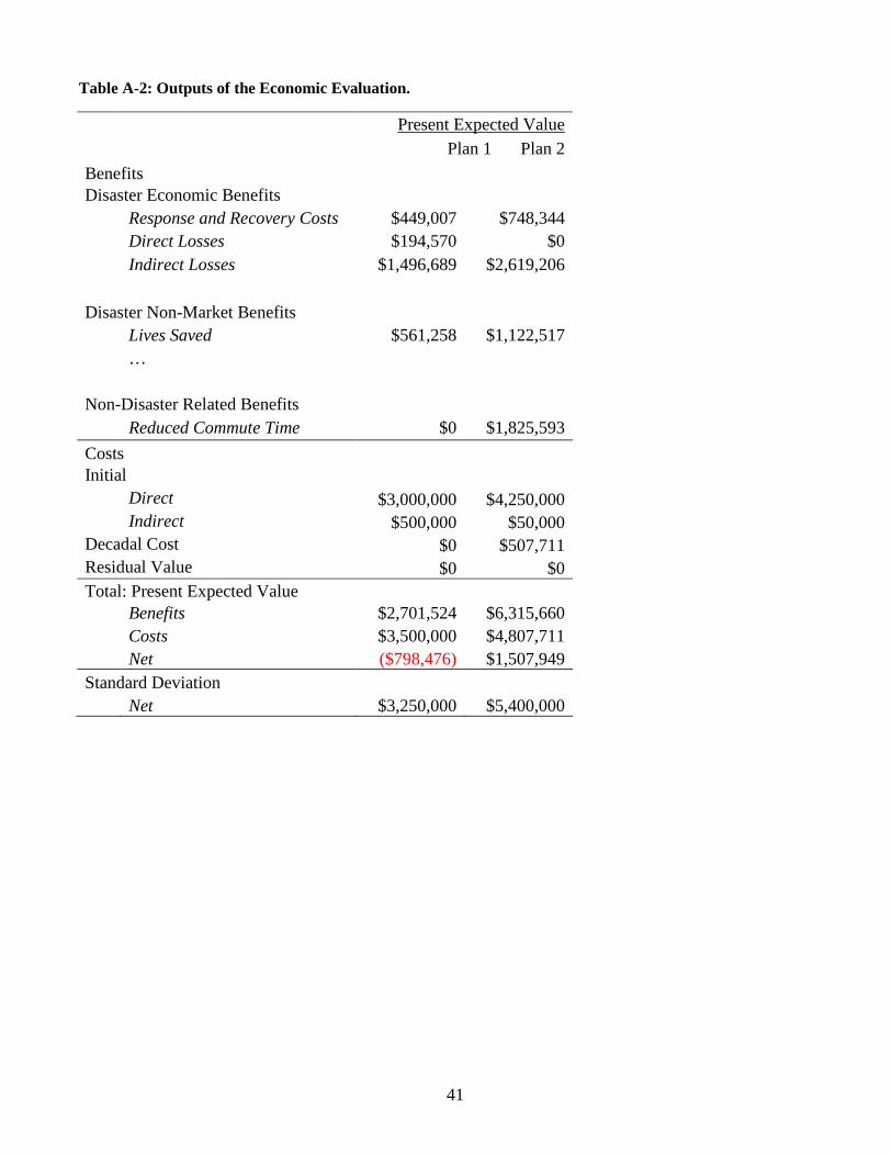
41

Table A-2: Outputs of the Economic Evaluation.

Present Expected Value Plan 1 Plan 2 Benefits Disaster Economic Benefits

Response and Recovery Costs $449,007 $748,344 Direct Losses $194,570 $0 Indirect Losses $1,496,689 $2,619,206

Disaster Non-Market Benefits

Lives Saved $561,258 $1,122,517 …

Non-Disaster Related Benefits

Reduced Commute Time $0 $1,825,593 Costs Initial

Direct $3,000,000 $4,250,000 Indirect $500,000 $50,000 Decadal Cost $0 $507,711 Residual Value $0 $0 Total: Present Expected Value Benefits $2,701,524 $6,315,660 Costs $3,500,000 $4,807,711 Net ($798,476) $1,507,949 Standard Deviation Net $3,250,000 $5,400,000

42

43

Appendix B: Exposition of Model This appendix contains a mathematical description of the Economic Guide model. It describes it in two forms, that of maximizing net benefits, and that of minimizing cost plus loss, and compares the two.

B.1. Maximizing Net Benefits Define

k Discount rate T𝑚𝑚𝑚𝑚𝑚𝑚 The (possibly infinite) Planning Period. P the set of all possible mitigation strategies. This includes any set of choices that could affect losses from disasters, including building codes, training of emergency response personnel, building and operation of an Emergency Operations Center, etc. P ∈ P some specific mitigation strategy. P0 ∈ P The status quo “mitigation strategy.” C( t, P) Costs as a function of time. Costs are specific to the mitigation strategy and are defined relative to the status quo. That is, by definition the costs associated with the status quo “strategy” are zero. {T𝑖𝑖, D𝑖𝑖(𝑃𝑃), R𝑖𝑖(𝑃𝑃)}𝑖𝑖=1∞ the sequence of disasters, where Ti is the time of the ith disaster, Di is the loss from the ith disaster, and Ri represents the response and recovery costs from the ith disaster. Loss and the response and recovery costs depend on the mitigation strategy. Since the disasters we are concerned about are in the future, this is a random sequence. 𝐼𝐼(T𝑚𝑚𝑚𝑚𝑚𝑚) = {𝑖𝑖|T𝑖𝑖 ≤ T𝑚𝑚𝑚𝑚𝑚𝑚} The set of disasters that fall within the planning period.

Then the Economic Framework attempts to solve this problem:

max𝑃𝑃∈𝒫𝒫

E � � ��D𝑖𝑖(𝑃𝑃0) − D𝑖𝑖(𝑃𝑃)� + �R𝑖𝑖(𝑃𝑃0) − R𝑖𝑖(𝑃𝑃)��𝑒𝑒−𝑘𝑘𝑘𝑘𝑖𝑖𝑖𝑖∈𝐼𝐼(T𝑚𝑚𝑚𝑚𝑚𝑚)

− � C(𝑡𝑡,𝑃𝑃)𝑒𝑒−𝑘𝑘𝑘𝑘𝑘𝑘≤T𝑚𝑚𝑚𝑚𝑚𝑚

�

(1)

where E represents the Expected Value operator. Results could be reported as either net savings 11 , a savings-to-investment ratio 12 , internal rate of return13, adjusted internal rate of return14 form, or all of the above. Since for most purposes these reporting approaches are equivalent, the reporting approach to use is the one that is most easily understood by the community’s decision-makers.

11 ASTM Standard E1074-09. 2009. 12 ASTM Standard E964-06 (2010). 2010. 13 ASTM Standard E1057-06 (2010). 2010. 14 ASTM Standard E1057-06 (2010). 2010.

44

Equation above is already expressed to show the net savings, as defined in ASTM Standard E1074-09. The savings-to-investment Ratio is defined by ASTM Standard 964-06 as

𝑆𝑆𝐼𝐼𝑆𝑆(𝑃𝑃) =∑ ��D𝑖𝑖(𝑃𝑃0) − D𝑖𝑖(𝑃𝑃)� + �R𝑖𝑖(𝑃𝑃0) − R𝑖𝑖(𝑃𝑃)��𝑒𝑒−𝑘𝑘𝑘𝑘𝑖𝑖𝑖𝑖∈𝐼𝐼(T𝑚𝑚𝑚𝑚𝑚𝑚)

∑ C(𝑡𝑡,𝑃𝑃)𝑒𝑒−𝑘𝑘𝑘𝑘𝑘𝑘≤T𝑚𝑚𝑚𝑚𝑚𝑚

The internal rate of return is defined by ASTM Standard E1057-06 as the value k*(P) such that:

E � � ��D𝑖𝑖(𝑃𝑃0) − D𝑖𝑖(𝑃𝑃)� + �R𝑖𝑖(𝑃𝑃0) − R𝑖𝑖(𝑃𝑃)��𝑒𝑒−𝑘𝑘∗(𝑃𝑃)𝑘𝑘𝑖𝑖

𝑖𝑖∈𝐼𝐼(T𝑚𝑚𝑚𝑚𝑚𝑚)

− � C(𝑡𝑡,𝑃𝑃)𝑒𝑒−𝑘𝑘∗(𝑃𝑃)𝑘𝑘

𝑘𝑘≤T𝑚𝑚𝑚𝑚𝑚𝑚

� = 0

Finally, the adjusted internal rate of return is defined by ASTM Standard E1057-06 as the value k*(P) such that:

E � � ��D𝑖𝑖(𝑃𝑃0) − D𝑖𝑖(𝑃𝑃)� + �R𝑖𝑖(𝑃𝑃0) − R𝑖𝑖(𝑃𝑃)��𝑒𝑒𝑟𝑟(𝑘𝑘𝑚𝑚𝑚𝑚𝑚𝑚−𝑘𝑘𝑖𝑖)−𝑘𝑘∗(𝑃𝑃)𝑘𝑘𝑚𝑚𝑚𝑚𝑚𝑚

𝑖𝑖∈𝐼𝐼(T𝑚𝑚𝑚𝑚𝑚𝑚)

− � C(𝑡𝑡,𝑃𝑃)𝑒𝑒𝑟𝑟(𝑘𝑘𝑚𝑚𝑚𝑚𝑚𝑚−𝑘𝑘𝑖𝑖)−𝑘𝑘∗(𝑃𝑃)𝑘𝑘𝑚𝑚𝑚𝑚𝑚𝑚

𝑘𝑘≤T𝑚𝑚𝑚𝑚𝑚𝑚

� = � 𝐼𝐼𝑘𝑘𝑒𝑒−𝑟𝑟𝑘𝑘𝑘𝑘≤T𝑚𝑚𝑚𝑚𝑚𝑚

Where Tmax is generally the planning period, r is the normal cost of capital or rate of return, and It is capital investment in time period t. Note that with the AIRR method some “costs” are synonymous with “investments.” B.2. Minimizing Cost Plus Loss In Cost-Plus-Loss terms, the Economic Framework attempts to solve this problem:

min𝑃𝑃∈𝒫𝒫

E � � [D𝑖𝑖(𝑃𝑃) + R𝑖𝑖(𝑃𝑃)]𝑒𝑒−𝑘𝑘𝑘𝑘𝑖𝑖𝑖𝑖∈𝐼𝐼(T𝑚𝑚𝑚𝑚𝑚𝑚)

+ � C(𝑡𝑡,𝑃𝑃)𝑒𝑒−𝑘𝑘𝑘𝑘𝑘𝑘≤T𝑚𝑚𝑚𝑚𝑚𝑚

� (2)

This is formally equivalent to the maximum-net-benefit formulation above. Here the objective is to reduce total costs from disasters. B.3. Computation and Discussion Two assumptions allow us to put the expectation in Equation (1) into a particularly simple form. Mathematical development is in Appendix C. Specifically, we assume that the probability of a disaster occurring (regardless of magnitude) is constant over time, and second we assume that the magnitude of a disaster, conditional on it occurring, is independent of the times between disasters and independent of the magnitude of previous disasters. To simplify exposition, the expected value of the total of disaster losses and response and recovery costs, conditional on a disaster occurring, and conditional on implementation of mitigation strategy P,

45

will be expressed as 𝐿𝐿�𝑃𝑃, and the variance of the total of disaster losses and response and recovery costs, conditional on a disaster occurring, and conditional on implementation of mitigation strategy P, will be expressed as 𝜎𝜎𝐿𝐿𝑃𝑃

2 . We also define λ as the rate of occurrence of a disaster, or equivalently, the inverse of the disaster return period. Further, define 𝐶𝐶� as the present expected value of the total of disaster losses and response and recovery costs for all disasters potentially occurring within the planning horizon. That is:

𝐶𝐶�(𝑃𝑃,𝑇𝑇𝑚𝑚𝑚𝑚𝑚𝑚, 𝜆𝜆, 𝑘𝑘) = � [D𝑖𝑖(𝑃𝑃) + R𝑖𝑖(𝑃𝑃)]𝑒𝑒−𝑘𝑘𝑘𝑘𝑖𝑖𝑖𝑖∈𝐼𝐼(T𝑚𝑚𝑚𝑚𝑚𝑚)

(3)

With those assumptions, the expected value and variance of disaster losses are:

𝐶𝐶�(𝑃𝑃,𝑇𝑇𝑚𝑚𝑚𝑚𝑚𝑚, 𝜆𝜆,𝑘𝑘) =𝜆𝜆𝑘𝑘

(1 − 𝑒𝑒−𝑘𝑘𝑘𝑘𝑚𝑚𝑚𝑚𝑚𝑚)𝐿𝐿�𝑃𝑃 (4)

and

𝜎𝜎2(𝑃𝑃,𝑇𝑇𝑚𝑚𝑚𝑚𝑚𝑚, 𝜆𝜆, 𝑘𝑘) =𝜆𝜆

2𝑘𝑘(1 − 𝑒𝑒−2𝑘𝑘𝑘𝑘𝑚𝑚𝑚𝑚𝑚𝑚)�𝜎𝜎𝐿𝐿𝑃𝑃

2 + 𝐿𝐿�𝑃𝑃2 � (5)

For the case where 𝑇𝑇𝑚𝑚𝑚𝑚𝑚𝑚 is infinite, this becomes:

𝐶𝐶�(𝑃𝑃,∞, 𝜆𝜆,𝑘𝑘) =𝜆𝜆𝑘𝑘𝐿𝐿�𝑃𝑃 (6)

and

𝜎𝜎2(𝑃𝑃,∞, 𝜆𝜆,𝑘𝑘) =𝜆𝜆

2𝑘𝑘�𝜎𝜎𝐿𝐿𝑃𝑃

2 + 𝐿𝐿�𝑃𝑃2 � (7)

And for the case where the discount factor k goes to zero, this becomes:

𝐶𝐶�(𝑃𝑃,𝑇𝑇𝑚𝑚𝑚𝑚𝑚𝑚 , 𝜆𝜆, 0) = 𝜆𝜆𝑇𝑇𝑚𝑚𝑚𝑚𝑚𝑚𝐿𝐿�𝑃𝑃 (8)

and 𝜎𝜎2(𝑃𝑃,𝑇𝑇𝑚𝑚𝑚𝑚𝑚𝑚, 𝜆𝜆, 0) = 𝜆𝜆𝑇𝑇𝑚𝑚𝑚𝑚𝑚𝑚�𝜎𝜎𝐿𝐿𝑃𝑃

2 + 𝐿𝐿�𝑃𝑃2 � (9)

Then, assuming costs are known, the present expected value of net benefits is.

𝐶𝐶�(𝑃𝑃0,𝑇𝑇𝑚𝑚𝑚𝑚𝑚𝑚, 𝜆𝜆,𝑘𝑘) − 𝐶𝐶�(𝑃𝑃,𝑇𝑇𝑚𝑚𝑚𝑚𝑚𝑚, 𝜆𝜆,𝑘𝑘) − 𝐶𝐶̅ =𝜆𝜆𝑘𝑘

(1 − 𝑒𝑒−𝑘𝑘𝑘𝑘𝑚𝑚𝑚𝑚𝑚𝑚)�𝐿𝐿�𝑃𝑃0 − 𝐿𝐿�𝑃𝑃� − 𝐶𝐶̅ (10)

And the present expected value of total costs is

𝐶𝐶�(𝑃𝑃,𝑇𝑇𝑚𝑚𝑚𝑚𝑚𝑚, 𝜆𝜆,𝑘𝑘) + 𝐶𝐶̅ =𝜆𝜆𝑘𝑘

(1 − 𝑒𝑒−𝑘𝑘𝑘𝑘𝑚𝑚𝑚𝑚𝑚𝑚)𝐿𝐿�𝑃𝑃 + 𝐶𝐶̅ (11)

Where 𝐶𝐶̅ is the present expected value of the costs of implementing the mitigation strategy.

46

To interpret these expressions it helps to understand that 𝜆𝜆�𝐿𝐿�𝑃𝑃0 − 𝐿𝐿�𝑃𝑃� represents the change in average annual disaster losses and recovery costs from the status quo, and �𝐿𝐿�𝑃𝑃0 − 𝐿𝐿�𝑃𝑃�𝜆𝜆𝑇𝑇 represents the change in the average amount of disaster losses and recovery costs over T years. So what this means is that given the assumptions listed above, a mitigation measures is worthwhile if the present value of its costs is less than the average losses expected to occur during the lifetime of the mitigation measure. The assumptions mentioned above are certainly incorrect, but their impact on the overall results is likely to be minimal. Weather-related hazards are correlated across time, and fire and geologic events tend to have reduced probabilities of occurrence after major events. Nevertheless, given the information that is likely to be available, these assumptions are likely to provide as good an approximation to the actual disaster sequence as any other that could be made. II.4. Sensitivity Analysis When we evaluate the sensitivity of these expressions, we are primarily interested in the effect of the parameters on the expected values. Table B-1 expresses the derivative (slope) of the expected value for each of the three cases in terms of the four main input parameters. Table B-1: Derivatives of value and scaled derivatives of value with respect to parameters. Case General Case k = 0 Tmax → ∞

Expression 𝜆𝜆𝑘𝑘

(1 − 𝑒𝑒−𝑘𝑘𝑘𝑘𝑚𝑚𝑚𝑚𝑚𝑚)𝐿𝐿�𝑃𝑃 𝜆𝜆𝑇𝑇𝑚𝑚𝑚𝑚𝑚𝑚𝐿𝐿�𝑃𝑃 𝜆𝜆𝑘𝑘𝐿𝐿�𝑃𝑃

𝒅𝒅𝒅𝒅𝒅𝒅𝒅𝒅

𝒅𝒅𝒅𝒅𝒅𝒅𝒅𝒅𝒅𝒅𝒅𝒅

𝒅𝒅𝒅𝒅𝒅𝒅𝒅𝒅

𝒅𝒅𝒅𝒅𝒅𝒅𝒅𝒅𝒅𝒅𝒅𝒅

𝒅𝒅𝒅𝒅𝒅𝒅𝒅𝒅

𝒅𝒅𝒅𝒅𝒅𝒅𝒅𝒅𝒅𝒅𝒅𝒅

λ 1𝑘𝑘

(1 − 𝑒𝑒−𝑘𝑘𝑘𝑘𝑚𝑚𝑚𝑚𝑚𝑚)𝐿𝐿�𝑃𝑃 1 𝑇𝑇𝑚𝑚𝑚𝑚𝑚𝑚𝐿𝐿�𝑃𝑃 1 𝐿𝐿�𝑃𝑃𝑘𝑘

1

Tmax 𝜆𝜆𝐿𝐿�𝑃𝑃𝑒𝑒−𝑘𝑘𝑘𝑘𝑚𝑚𝑚𝑚𝑚𝑚 𝑒𝑒−𝑘𝑘𝑘𝑘𝑚𝑚𝑚𝑚𝑚𝑚

1 − 𝑒𝑒−𝑘𝑘𝑘𝑘𝑚𝑚𝑚𝑚𝑚𝑚𝑘𝑘𝑇𝑇𝑚𝑚𝑚𝑚𝑚𝑚 𝜆𝜆𝐿𝐿�𝑃𝑃 1 -- --

𝐿𝐿�𝑃𝑃 𝜆𝜆𝑘𝑘

(1 − 𝑒𝑒−𝑘𝑘𝑘𝑘𝑚𝑚𝑚𝑚𝑚𝑚) 1 𝜆𝜆𝑇𝑇𝑚𝑚𝑚𝑚𝑚𝑚 1 𝜆𝜆𝑘𝑘

1

k − 𝜆𝜆𝑘𝑘2

(1 − (1 + 𝑘𝑘𝑇𝑇𝑚𝑚𝑚𝑚𝑚𝑚)𝑒𝑒−𝑘𝑘𝑘𝑘𝑚𝑚𝑚𝑚𝑚𝑚)𝐿𝐿�𝑃𝑃1 𝑒𝑒−𝑘𝑘𝑘𝑘𝑚𝑚𝑚𝑚𝑚𝑚

1 − 𝑒𝑒−𝑘𝑘𝑘𝑘𝑚𝑚𝑚𝑚𝑚𝑚𝑘𝑘𝑇𝑇𝑚𝑚𝑚𝑚𝑚𝑚 − 1 -- -- −

𝜆𝜆𝑘𝑘2𝐿𝐿�𝑃𝑃 -1

1 Note that lim𝑘𝑘→0 −𝑑𝑑𝑉𝑉𝑑𝑑𝑘𝑘

= − 𝜆𝜆𝑘𝑘𝑚𝑚𝑚𝑚𝑚𝑚2

2𝑆𝑆̅(𝑃𝑃)

Increasing k decreases the sensitivity, while increasing λ, μ, and 𝑆𝑆̅ increases sensitivity. Increasing Tmax increases sensitivity to all terms except Tmax itself, where increasing Tmax actually decreases the sensitivity.

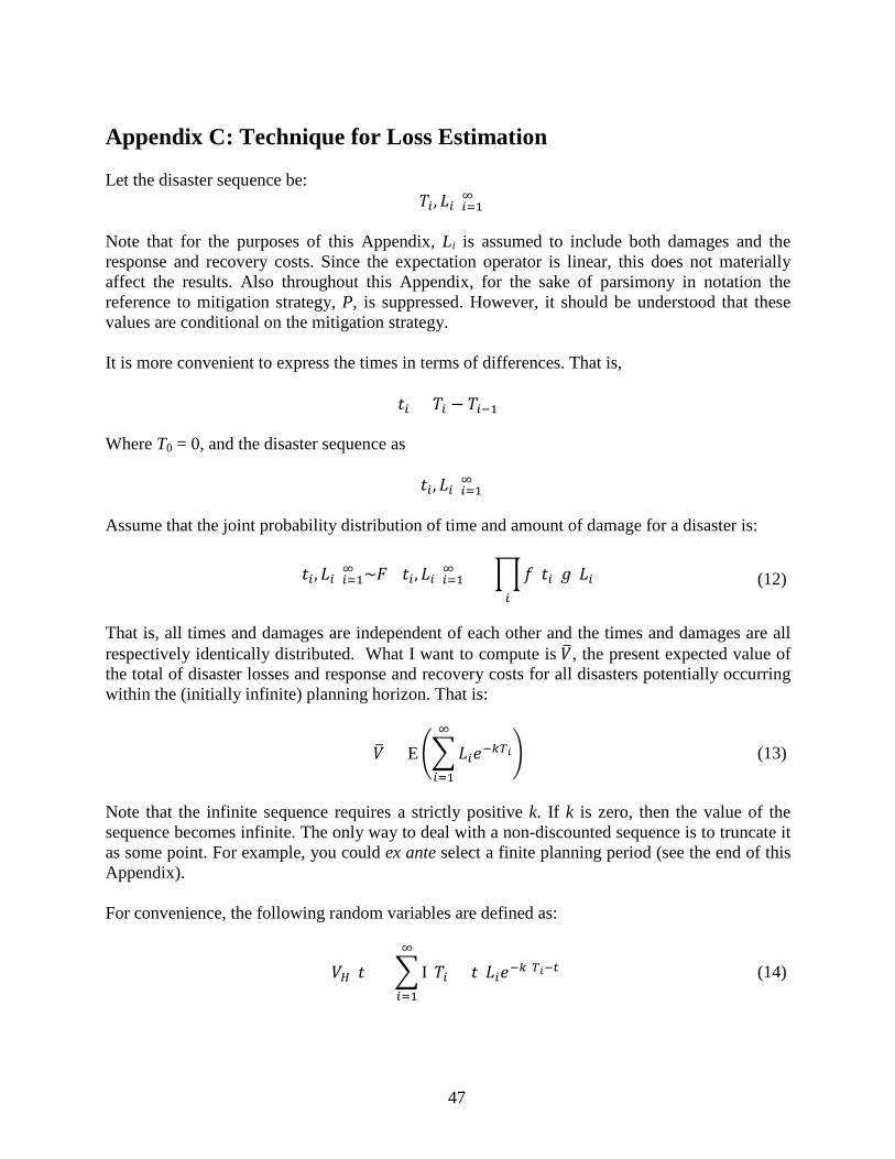
47

Appendix C: Technique for Loss Estimation Let the disaster sequence be:

{𝑇𝑇𝑖𝑖, 𝐿𝐿𝑖𝑖}𝑖𝑖=1∞ Note that for the purposes of this Appendix, Li is assumed to include both damages and the response and recovery costs. Since the expectation operator is linear, this does not materially affect the results. Also throughout this Appendix, for the sake of parsimony in notation the reference to mitigation strategy, P, is suppressed. However, it should be understood that these values are conditional on the mitigation strategy. It is more convenient to express the times in terms of differences. That is,

𝑡𝑡𝑖𝑖 = 𝑇𝑇𝑖𝑖 − 𝑇𝑇𝑖𝑖−1 Where T0 = 0, and the disaster sequence as

{𝑡𝑡𝑖𝑖, 𝐿𝐿𝑖𝑖}𝑖𝑖=1∞ Assume that the joint probability distribution of time and amount of damage for a disaster is:

{𝑡𝑡𝑖𝑖, 𝐿𝐿𝑖𝑖}𝑖𝑖=1∞ ~𝐹𝐹({𝑡𝑡𝑖𝑖, 𝐿𝐿𝑖𝑖}𝑖𝑖=1∞ ) = �𝑓𝑓(𝑡𝑡𝑖𝑖)𝑔𝑔(𝐿𝐿𝑖𝑖)𝑖𝑖

(12)

That is, all times and damages are independent of each other and the times and damages are all respectively identically distributed. What I want to compute is 𝐶𝐶� , the present expected value of the total of disaster losses and response and recovery costs for all disasters potentially occurring within the (initially infinite) planning horizon. That is:

𝐶𝐶� = E��𝐿𝐿𝑖𝑖𝑒𝑒−𝑘𝑘𝑘𝑘𝑖𝑖∞

𝑖𝑖=1

� (13)

Note that the infinite sequence requires a strictly positive k. If k is zero, then the value of the sequence becomes infinite. The only way to deal with a non-discounted sequence is to truncate it as some point. For example, you could ex ante select a finite planning period (see the end of this Appendix). For convenience, the following random variables are defined as:

𝐶𝐶𝐻𝐻(𝑡𝑡) = � I{𝑇𝑇𝑖𝑖 > 𝑡𝑡}𝐿𝐿𝑖𝑖𝑒𝑒−𝑘𝑘(𝑘𝑘𝑖𝑖−𝑘𝑘)∞

𝑖𝑖=1

(14)

48

𝐶𝐶𝐿𝐿(𝑡𝑡) = � I{𝑇𝑇𝑖𝑖 ≤ 𝑡𝑡}𝐿𝐿𝑖𝑖𝑒𝑒−𝑘𝑘(𝑘𝑘𝑖𝑖−𝑘𝑘)∞

𝑖𝑖=1

(15)

𝐶𝐶𝑛𝑛 = �𝐿𝐿𝑖𝑖𝑒𝑒−𝑘𝑘(𝑘𝑘𝑖𝑖−𝑘𝑘𝑛𝑛−1)∞

𝑖𝑖=𝑛𝑛

(16)

where I{∙} is the indicator function. Equation (16) is used to rewrite 𝐶𝐶� as: 𝐶𝐶� = E{(𝐿𝐿1 + 𝐶𝐶2)𝑒𝑒−𝑘𝑘𝑘𝑘1} (17) Since all values for damage and time-between are independent of each other, then L1, T1, and V2 are independent of each other. So 𝐶𝐶� = �E(𝐿𝐿1) + E(𝐶𝐶2)�E{𝑒𝑒−𝑘𝑘𝑘𝑘1} (18) To simplify the expression, substitute in:

𝐸𝐸(𝐿𝐿1) = 𝐸𝐸(𝐿𝐿) = 𝐿𝐿� = � 𝑥𝑥𝑔𝑔(𝑥𝑥)𝑑𝑑𝑥𝑥∞

0

(19)

Which gives: 𝐶𝐶� = �𝐿𝐿� + 𝐸𝐸(𝐶𝐶2)�𝐸𝐸{𝑒𝑒−𝑘𝑘𝑘𝑘1} (20) Further, since the times-between and damages are all independent of each other, 𝐸𝐸(𝐶𝐶1) = 𝐸𝐸(𝐶𝐶2) = 𝐸𝐸(𝐶𝐶𝑖𝑖) = 𝐶𝐶� (21) That gives: 𝐶𝐶� = (𝐿𝐿� + 𝐶𝐶�)𝐸𝐸{𝑒𝑒−𝑘𝑘𝑘𝑘1} (22) Which can also be expressed as:

𝐶𝐶� = (𝐶𝐶� + 𝐿𝐿�)� 𝑒𝑒−𝑘𝑘𝑘𝑘𝑓𝑓(𝑇𝑇)𝑑𝑑𝑇𝑇∞

0

(23)

Since the occurrence of disasters is a Poisson process, then the time between events is an exponential distribution. Then this expression becomes:

𝐶𝐶� = (𝐶𝐶� + 𝐿𝐿�)� 𝜆𝜆𝑒𝑒−𝑘𝑘𝑘𝑘𝑒𝑒−𝜆𝜆𝑘𝑘𝑑𝑑𝑇𝑇∞

0

(24)

This yields:

𝐶𝐶� =𝜆𝜆

𝑘𝑘 + 𝜆𝜆(𝐶𝐶� + 𝐿𝐿�)�(𝑘𝑘 + 𝜆𝜆)𝑒𝑒−(𝑘𝑘+𝜆𝜆)𝑘𝑘𝑑𝑑𝑇𝑇

∞

0

𝐶𝐶� = −𝜆𝜆

𝑘𝑘 + 𝜆𝜆(𝐶𝐶� + 𝐿𝐿�)𝑒𝑒−(𝑘𝑘+𝜆𝜆)𝑘𝑘�

0

∞

49

𝐶𝐶� =𝜆𝜆

𝑘𝑘 + 𝜆𝜆(𝐶𝐶� + 𝐿𝐿�)

𝐶𝐶� �1 −𝜆𝜆

𝑘𝑘 + 𝜆𝜆� =

𝜆𝜆𝑘𝑘 + 𝜆𝜆

𝐿𝐿� (25)

Therefore:

𝐶𝐶� =𝜆𝜆𝑘𝑘𝐿𝐿� (26)

The present expected value of any disasters occurring before a specified point of time, t0, can be easily obtained by subtracting out the discounted value at time t0. That is,

𝐶𝐶�(𝑡𝑡) = E(𝐶𝐶1 − 𝐶𝐶𝐻𝐻(𝑡𝑡)𝑒𝑒−𝑘𝑘𝑘𝑘) = 𝐶𝐶� − 𝐶𝐶�𝑒𝑒−𝑘𝑘𝑘𝑘 =𝜆𝜆𝑘𝑘𝐿𝐿�(1 − 𝑒𝑒−𝑘𝑘𝑘𝑘) (27)

Variance can be determined similarly. Let

𝜎𝜎𝑉𝑉2 = Var(𝐶𝐶) = Var��𝐿𝐿𝑖𝑖𝑒𝑒−𝑘𝑘𝑘𝑘1∞

𝑖𝑖=𝑛𝑛

� (28)

Using the same trick as before, Equation (28) rewritten as: 𝜎𝜎𝑉𝑉2 = Var(𝐶𝐶) = Var{(𝐿𝐿1 + 𝐶𝐶2)𝑒𝑒−𝑘𝑘𝑘𝑘1} (29) Or 𝜎𝜎𝑉𝑉2 = E{(𝐿𝐿1 + 𝐶𝐶2)2𝑒𝑒−2𝑘𝑘𝑘𝑘1} − 𝐶𝐶�2 (30)

= E{(𝐿𝐿12 + 2𝐿𝐿1𝐶𝐶2 + 𝐶𝐶22)𝑒𝑒−2𝑘𝑘𝑘𝑘1} − 𝐶𝐶�2 (31)

= E��(𝐿𝐿12 − 𝐿𝐿�2) + 2𝐿𝐿1𝐶𝐶2 + (𝐶𝐶22 − 𝐶𝐶�2) + 𝐿𝐿�2 + 𝐶𝐶�2�𝑒𝑒−2𝑘𝑘𝑘𝑘1� − 𝐶𝐶�2 (32)

Again, independence allows an evaluation of the expectation of each term separately: = (E(𝐿𝐿12 − 𝐿𝐿�2) + 2E(𝐿𝐿1)E(𝐶𝐶2) + E(𝐶𝐶22 − 𝐶𝐶�2) + 𝐿𝐿2 + 𝐶𝐶�2)E{𝑒𝑒−2𝑘𝑘𝑘𝑘1} − 𝐶𝐶�2 (33)

= (𝜎𝜎𝐿𝐿2 + 2𝐿𝐿�𝐶𝐶� + E(𝐶𝐶22 − 𝐶𝐶�2) + 𝐿𝐿2 + 𝐶𝐶�2)E{𝑒𝑒−2𝑘𝑘𝑘𝑘1} − 𝐶𝐶�2 (34)

Where 𝜎𝜎𝐿𝐿2 = E(𝐿𝐿12 − 𝐿𝐿�2) = E(𝐿𝐿𝑖𝑖2 − 𝐿𝐿�2) (35) And again, because the infinite sequence where damages and times-between is independent: E(𝐶𝐶2 − 𝐶𝐶�2) = E(𝐶𝐶12 − 𝐶𝐶�2) = E(𝐶𝐶22 − 𝐶𝐶�2) = E(𝐶𝐶𝑖𝑖2 − 𝐶𝐶�2) = 𝜎𝜎𝑉𝑉2 (36) So equation (34) becomes 𝜎𝜎𝑉𝑉2 = (𝜎𝜎𝐿𝐿2 + 𝜎𝜎𝑉𝑉2 + 𝐿𝐿�2 + 2𝐿𝐿�𝐶𝐶� + 𝐶𝐶�2)E{𝑒𝑒−2𝑘𝑘𝑘𝑘1} − 𝐶𝐶�2 (37)

50

Again, since times-between follow an exponential distribution, this becomes

𝜎𝜎𝑉𝑉2 = (𝜎𝜎𝐿𝐿2 + 𝜎𝜎𝑉𝑉2 + 𝐿𝐿�2 + 2𝐿𝐿�𝐶𝐶� + 𝐶𝐶�2)� 𝜆𝜆𝑒𝑒−2𝑘𝑘𝑘𝑘𝑒𝑒−𝜆𝜆𝑘𝑘𝑑𝑑𝑇𝑇∞

0

− 𝐶𝐶�2 (38)

𝜎𝜎𝑉𝑉2 =𝜆𝜆

2𝑘𝑘 + 𝜆𝜆(𝜎𝜎𝐿𝐿2 + 𝜎𝜎𝑉𝑉2 + 𝐿𝐿�2 + 2𝐿𝐿�𝐶𝐶� + 𝐶𝐶�2)�(2𝑘𝑘 + 𝜆𝜆)𝑒𝑒−(2𝑘𝑘+𝜆𝜆)𝑘𝑘𝑑𝑑𝑇𝑇

∞

0

− 𝐶𝐶�2 (39)

𝜎𝜎𝑉𝑉2 =𝜆𝜆

2𝑘𝑘 + 𝜆𝜆(𝜎𝜎𝐿𝐿2 + 𝜎𝜎𝑉𝑉2 + 𝐿𝐿�2 + 2𝐿𝐿�𝐶𝐶� + 𝐶𝐶�2) − 𝐶𝐶�2 (40)

Or

𝜎𝜎𝑉𝑉2 �1 −𝜆𝜆

2𝑘𝑘 + 𝜆𝜆� =

𝜆𝜆2𝑘𝑘 + 𝜆𝜆

(𝜎𝜎𝐿𝐿2 + 𝐿𝐿�2 + 2𝐿𝐿�𝐶𝐶�) − 𝐶𝐶�2 �1 −𝜆𝜆

2𝑘𝑘 + 𝜆𝜆� (41)

𝜎𝜎𝑉𝑉22𝑘𝑘

2𝑘𝑘 + 𝜆𝜆=

𝜆𝜆2𝑘𝑘 + 𝜆𝜆

(𝜎𝜎𝐿𝐿2 + 𝐿𝐿�2 + 2𝐿𝐿�𝐶𝐶�) − 𝐶𝐶�22𝑘𝑘

2𝑘𝑘 + 𝜆𝜆 (42)

𝜎𝜎𝑉𝑉2 =𝜆𝜆

2𝑘𝑘(𝜎𝜎𝐿𝐿2 + 𝐿𝐿�2 + 2𝐿𝐿�𝐶𝐶�) − 𝐶𝐶�2 (43)

Substitute the expression for 𝐶𝐶� from equation (26):

𝜎𝜎𝑉𝑉2 =𝜆𝜆

2𝑘𝑘�𝜎𝜎𝐿𝐿2 + 𝐿𝐿�2 + 2𝐿𝐿�

𝜆𝜆𝑘𝑘𝐿𝐿�� − �

𝜆𝜆𝑘𝑘𝐿𝐿��

2

(44)

𝜎𝜎𝑉𝑉2 =𝜆𝜆

2𝑘𝑘𝜎𝜎𝐿𝐿2 +

𝜆𝜆2𝑘𝑘

�𝑘𝑘 + 2𝜆𝜆𝑘𝑘

� 𝐿𝐿2 −𝜆𝜆2

𝑘𝑘�2𝐿𝐿�2 (45)

𝜎𝜎𝑉𝑉2 =𝜆𝜆

2𝑘𝑘𝜎𝜎𝐿𝐿2 + �

𝜆𝜆2𝑘𝑘

+𝜆𝜆2

𝑘𝑘�2−𝜆𝜆2

𝑘𝑘�2� 𝐿𝐿�2 (46)

Or,

𝜎𝜎𝑉𝑉2 =𝜆𝜆

2𝑘𝑘𝜎𝜎𝐿𝐿2 +

𝜆𝜆2𝑘𝑘

𝐿𝐿�2 =𝜆𝜆

2𝑘𝑘(𝜎𝜎𝐿𝐿2 + 𝐿𝐿�2) (47)

Again, to get the variance for a fixed time interval V is partitioned and variance taken: 𝜎𝜎𝑉𝑉2 = Var(𝐶𝐶) = Var(𝐶𝐶𝐿𝐿(𝑡𝑡) + 𝐶𝐶𝐻𝐻(𝑡𝑡)𝑒𝑒−𝑘𝑘𝑘𝑘) (48) Since 𝐶𝐶𝐿𝐿(𝑡𝑡) and 𝐶𝐶𝐻𝐻(𝑡𝑡) are independent for fixed t, and for any two independent random variables, X and Y, Var(𝑋𝑋 + 𝑌𝑌) = Var(𝑋𝑋) + Var(𝑌𝑌), this becomes: 𝜎𝜎𝑉𝑉2 = Var�𝐶𝐶𝐿𝐿(𝑡𝑡)� + Var(𝐶𝐶𝐻𝐻(𝑡𝑡)𝑒𝑒−𝑘𝑘𝑘𝑘) (49) Note that 𝜎𝜎𝑉𝑉2(𝑡𝑡) = 𝐶𝐶𝑉𝑉𝑟𝑟�𝐶𝐶𝐿𝐿(𝑡𝑡)� is the expression of interest:

51

𝜎𝜎𝑉𝑉2 = 𝜎𝜎𝑉𝑉2(𝑡𝑡) + Var(𝐶𝐶𝐻𝐻(𝑡𝑡)𝑒𝑒−𝑘𝑘𝑘𝑘) (50) Since t is fixed and non-stochastic: 𝜎𝜎𝑉𝑉2 = 𝜎𝜎𝑉𝑉2(𝑡𝑡) + �E ��𝐶𝐶𝐻𝐻(𝑡𝑡)�

2� − (E{𝐶𝐶𝐻𝐻(𝑡𝑡)})2� 𝑒𝑒−2𝑘𝑘𝑘𝑘 (51)

𝜎𝜎𝑉𝑉2 = 𝜎𝜎𝑉𝑉2(𝑡𝑡) + Var�𝐶𝐶𝐻𝐻(𝑡𝑡)�𝑒𝑒−2𝑘𝑘𝑘𝑘 (52)

And as noted above, 𝜎𝜎𝑉𝑉2 = 𝐶𝐶𝑉𝑉𝑟𝑟�𝐶𝐶𝐻𝐻(𝑡𝑡)�, so 𝜎𝜎𝑉𝑉2 = 𝜎𝜎𝑉𝑉2(𝑡𝑡) + 𝜎𝜎𝑉𝑉2𝑒𝑒−2𝑘𝑘𝑘𝑘 (53) Or

𝜎𝜎𝑉𝑉2(𝑡𝑡) = 𝜎𝜎𝑉𝑉2(1 − 𝑒𝑒−2𝑘𝑘𝑘𝑘) =𝜆𝜆

2𝑘𝑘(𝜎𝜎𝐿𝐿2 + 𝐿𝐿2)(1 − 𝑒𝑒−2𝑘𝑘𝑘𝑘) (54)

As far as the case where k = 0, the following limit argument gives an expression for 𝐶𝐶�(𝑡𝑡) and 𝜎𝜎𝑉𝑉2(𝑡𝑡) when k = 0. Starting with

𝐶𝐶�(𝑡𝑡) =𝜆𝜆𝑘𝑘𝐿𝐿�(1 − 𝑒𝑒−𝑘𝑘𝑘𝑘) (18)

Expand the Taylor series for the exponential term:

𝐶𝐶�(𝑡𝑡) ≈𝜆𝜆𝑘𝑘𝐿𝐿� �1 − �1 − 𝑘𝑘𝑡𝑡 +

𝑘𝑘2𝑡𝑡2

2!�� =

𝜆𝜆𝑘𝑘𝐿𝐿� �𝑘𝑘𝑡𝑡 −

𝑘𝑘2𝑡𝑡2

2!� (55)

𝐶𝐶�(𝑡𝑡) ≈ 𝜆𝜆𝐿𝐿� �𝑡𝑡 −𝑘𝑘𝑡𝑡2

2!� (56)

Take the limit as k → 0, this becomes lim

𝑘𝑘→0𝐶𝐶�(𝑡𝑡) = 𝐿𝐿�𝜆𝜆𝑡𝑡 (57)

Similarly for 𝜎𝜎𝑉𝑉2(𝑡𝑡), we get:

𝜎𝜎𝑉𝑉2(𝑡𝑡) =𝜆𝜆

2𝑘𝑘(𝜎𝜎𝐿𝐿2 + 𝐿𝐿�2)(1− 𝑒𝑒−2𝑘𝑘𝑘𝑘) ≈

𝜆𝜆2𝑘𝑘

(𝜎𝜎𝐿𝐿2 + 𝐿𝐿�2)�1 − �1 − 2𝑘𝑘𝑡𝑡 +4𝑘𝑘2𝑡𝑡2

2!�� (58)

𝜎𝜎𝑉𝑉2(𝑡𝑡) ≈𝜆𝜆

2𝑘𝑘(𝜎𝜎𝐿𝐿2 + 𝐿𝐿�2)�2𝑘𝑘𝑡𝑡 −

4𝑘𝑘2𝑡𝑡2

2!� = 𝜆𝜆(𝜎𝜎𝐿𝐿2 + 𝐿𝐿�2) �𝑡𝑡 −

2𝑘𝑘𝑡𝑡2

2!� (59)

So lim

𝑘𝑘→0𝜎𝜎𝑉𝑉2(𝑡𝑡) = (𝜎𝜎𝐿𝐿2 + 𝐿𝐿�2)𝜆𝜆𝑡𝑡 (60)

52