Embed Size (px)
Citation preview
JPL Publication 94-8
Communications and Control
for Electric Power Systems:
Power System Stability Applicationsof Artificial Neural Networks
N. Toomarian
H. Kirkham
April 1994
Prepared for
Office of Energy Management SystemsUnited States Department of Energy
Through an agreement with
National Aeronautics and
Space Administration
by
Jet Propulsion LaboratoryCalifornia Institute of TechnologyPasadena, California
https://ntrs.nasa.gov/search.jsp?R=19950015754 2018-06-25T14:04:48+00:00Z


Prepared by the Jet Propulsion Laboratory, California Institute of Technology,for the U.S. Department of Energy through an agreement with the National
Aeronautics and Space Administration.
This report was prepared as an account of work sponsored by an
agency of the United States Government. Neither the United States Governmentnor any agency thereof, nor any of their employees, makes any warranty,
express or implied, or assumes any legal liability or responsibility for the
accuracy, completeness, or usefulness of any information, apparatus, product,
or process disclosed, or represents that its use would not infringe privately
owned rights.Reference herein to any specific commercial product, process, or
service by trade name, trademark, manufacturer, or otherwise, does not
necessarily constitute or imply its endorsement, recommendation, or favoringby the United States Government or any agency thereof.
This publication reports on work performed under NASA Task RE-152,
Amendment 203 and sponsored through DOE/NASA Interagency AgreementNo. DE-AI01-79ET 29372 (Mod. A009).


ABSTRACT
HIS REPORT investigates the application of artificial neural networks to the problem ofpower system stability. The field of artificial intelligence, expert systems and neural
networks is reviewed. Power system operation is discussed with emphasis on stability consider-
ations. Real-time system control has only recently been considered as applicable to stability,
using conventional control methods. The report considers the use of artificial neural networks
to improve the stability of the power system. The networks are considered as adjuncts and as
replacements for existing controllers. The optimal kind of network to use as an adjunct to a
generator exciter is discussed.
iii


FOREWORD
HIS REPORT discusses the application of the relatively new technology of artificial neuralnetworks to one of the oldest problems of electric power systems: stability. Power systems
are nonlinear in certain respects, and that means that instability of various kinds is possible. The
instability considered in this report is the kind demonstrated in the New York blackout of 1965.
While the problem is an old one, it is likely to be of increasing importance to find a
solution. A number of evolutionary pressures are acting now so as to change radically the nature
of the industry. These were reviewed at a meeting organized by the Department of Energy
(DOE) in Denver, Colorado, in March 1990. Real-time control and operation were considered
in detail at a DOE Workshop, also in Denver, in November 1991. At the first meeting, the
factors affecting the evolution of the industry were thought to include:
• the regulatory process
• industry competitiveness
• new technologies
• load growth
• renewable sources and storage• environmental concerns.
Because of the first three of these factors, it was estimated that by 2020 over 50 % of new
generation would be non-utility owned, and transmission line loading would be high. These are
the ingredients for trouble. The report of the first Denver meeting concluded that blackouts and
brownouts would occur if existing control devices and operating practices continued to be used.
The work described in this report is aimed at developing new control devices and operat-
ing practices that may contribute to forestalling the difficulties seen for the future power system.
Given the lead-time required to put any new technology into practice, it is not too early to start
investigating such advanced concepts as controllers based on artificial neural networks. Our work
shows that neural nets could be a valuable addition to the options available for power system
operation.
Because we are mixing two disparate technologies, power systems and neural nets, some
background material on both topics is included in this report. The reader who feels the need to
brush up on either topic should find help in Part 1 or Part 2 of the report. The reader who is
comfortable in both areas may skip directly to Part 3.
HAROLD KIRKHAM
PASADENA, CALIFORNIA
APRIL 1994
V
PRC,-4NIE)_Ne PIIGE ltLANK NOT FIRMED


TABLE OF CONTENTS
ABSTRACT ............................................... iii
FOREWORD .............................................. v
PART 1. POWER SYSTEM STABILITY ............................ 1
PART 2: NEURAL NETWORKS ................................. 9
AI Modeling and Neural Networks ............................. 11
A History of Artificial Neural Networks .......................... 13
Computational Neural Learning ............................... 16
Adaptive Neural Control System Architectures ....................... 18
Direct Implementation .................................. 20
Indirect Implementation .................................. 21
Summary .......................................... 22
Neural Hardware Implementation ............................... 23Conclusions ............................................ 26
PART 3. APPLICATION ...................................... 29
Application of Neural Networks ............................... 32
Future Work: Feasibility Study and Network Selection ................. 34
APPENDIX A. NEURAL LEARNING FORMALISM .................... 37
REFERENCES ............................................. 43
vii
__c_ PAGE BLANK NOT FILMED

LIST OF FIGURES
Figure Page
1-1. Simple power system ...................................... 2
1-2. Respecified system ........................................ 3
1-3. Machine and infinite bus .................................... 5
1-4. Power-angle curve ........................................ 7
2-1.
2-2.
2-3.
2-4.
2-5.
2-6.
Model of a neural system .................................... 14
Biological neuron ........................................ 15
Functional model of simulated neuron ............................ 16
Direct adaptive control ..................................... 20
Indirect adaptive control .................................... 22
Computational capabilities of some biological systems .................. 24
3-1.
3-2.
3-3.
3-4.
Simple power system ...................................... 30
Generator controls ........................................ 31
3-machine power system .................................... 32
Power system stabilizer with neural network ........................ 33
A-1. Topology of a general network ................................ 38
.°oVUl

PART 1. POWER SYSTEM STABILITY
tOWER SYSTEM OPERATION is a complex topic. The way energy flows in an inter-connected network is not obvious, and difficult to analyze even in the steady state. The fact
that the system is nonlinear can lead to instability. The objective of maintaining high reliability
of service in spite of these features of the system have led, over the years, to some conservative
ways of operating.
It seems fair to ask why the electric power system presents a problem in determining load
flow. After all, the components of the power system, the lines, transformers and generators, are
all well-understood devices. In part the difficulty stems from the fact that the load on the system
is not known. It can be said that the load is not simply resistive, and is distributed geographical-
ly, but its power demand is not known, or indeed directly measurable. Another part of the
problem arises from the way the system parameters are specified. An example will illustrate the
point.
Consider the simple system shown in Figure 1-1. There are two generators, a single load,
and two resistors representing the losses in the transmission lines. (Although most power systems
are ac, we can demonstrate the analytical difficulties more clearly with a dc system, as shown.)
We begin by specifying that the left generator output is 100 W, and the load power is
150 W at 100 V. (This kind of specification of the generation is reasonably representative of
power system practice. The left generator might be a small efficient unit, running at full power.)
JPL 94-8, page 1

Part 1: PowerSystem Stability
The problem is to determine the bus voltages V s and V3 and the power to be delivered
by the right generator. When these three quantities are known, the system operating conditionswill be known.
Figure 1-1. SSimple power system
11 10 V2= 100V 10 13
Pt2
LOAD
150W
00W
V 3
P
)
The load current is
Two expressions can be written for/1:
/1 =_
and
from which 11 = Vs - 100.
150W -1.5A (1-1)/2- lOOV
100
171 (1-2)
}'1 -V2 (1-3)Is= 1
The voltage VI of the left generator is uniquely specified because
100 =Vx-100vl
or
This may be solved directly
Of course,
By Kirchoff's Current Law,
and we can solve for I3:
(1-4)
V12 - 100V s - 100 =0 (1-5)
V 1 = 100.99V (1-6)
I s = 10---0-0=0.99A (1-7)vl
I2 =I s+I 3 (1-8)
13=12 -11 = 1.50 - 0.99 =0.51 A (1-9)
}'3 can be found by considering the volt-drop due to 13 in the 1 0 line resistance. The
result is V3 = 100.51 V. Now the power from the right generator can be found:
P, = V313 =51.26W (1-10)
JPL 94-8, page 2

Part 1- Power System Stability
The system is now completely analyzed. The right generator must burn enough fuel to
generate 51.26 W, and the field current must be adjusted for a terminal voltage of 100.51 V.
The left generator must supply 100 W at 100.99 V.
Although the system is extremely simple, the above analysis illustrates some important
concepts. In the real world, the exact power of the load is not generally known. In scheduling
the generation, one generator is designated as the "slack" machine (the right hand generator in
the example), characterized by an initially unknown power generation. The power is then
adjusted so that the frequency is at the required value: by definition the demand is then being
met.
The purpose of a load flow calculation such as the one above is to determine the voltages
and power flows throughout the system, based on the measured data. There are 5 degrees of
freedom in the circuit of Figure 1-1. In other words, the specification of five independent
quantities serves to totally determine the behavior of the system. In our example, the five
quantities were the power of the left generator, the power of the load, the load voltage and the
two line resistances. These are not the traditionally specified parameters. The load is
geographically distributed, and is voltage dependent. Load power is therefore not known, butmust be found in a load flow calculation.
The specification of different parameters has a profound effect on the calculation. Let us
solve the system again with the following parameters specified: the power of the left generator,
the two line resistances, the power at the load and the voltage at the right generator. This system
is shown in Figure 1-2.
Figure 1-2. SRespecified system \
I 1_
y°V2
12
LOAD
150W
lt3 13 V3- IOOV
P
We proceed in a straightforward fashion to determine the power to be supplied by the
right generator as well as the two remaining bus voltages 111and V2.
e (1-11)/3--
eV2_- 100- 113 = 100-_ (1-12)
100
P_o_ = V212= 150 (1-13)
2 _
150
[100
JPL 94-8, page 3

Part 1: PowerSystem Stability
[1 =[2 -[3 =150 P
[ 100 - -i-_p] 100 (1-15)
150 P+ - _ (1-16)
[Io0-P] 100
P_. = 100 = 1/'1/_ (1-17)
Substituting for 1"1, 11 in this equation yields one equation involving P that we can use
to determine system operating point. The equation is a fourth order polynomial in P. Numericalevaluation leads to
P=51.25W
The other values follow immediately:
I3 =0.5125A
Vz =99.4875V, I2 =1.5077A
V 1 =100.4827A, I_ =0.9952A
(1-18)
(1-19)
(1-20)
The analytic complexity of the solution is masked by the few lines above indicating that
the equation is a fourth order polynomial in P. Although this second problem appears to be a
minor variation of the first (indeed the final values for the current, voltage and power are not
significantly different), the mathematical complexity is such as to require numerical techniques.
And this is for a system with only five degrees of freedom[ A real power system will have
several thousand degrees of freedom, and will be specified in the way our second example wasspecified. Numerical methods are clearly called for.
We have seen how difficult it is to fix the steady-state operating point of a power system.
Now let us turn to the dynamics of the system.
Once more, we will illustrate the problem by means of an example. Consider another
simple power system, consisting of one machine and an infinite bus 1, connected by two
transmission lines, as shown in Figure 1-3.
z An infinite bus is a hypothetical convenience. It is a connection point defined so that whatever
power is inserted into it (or taken out of it), the frequency and the voltage remain constant. This has the
advantage for our purposes that it makes the equations of motion of the system much simpler. (In
practice, as far as any single generator in a power system is concemed, the remainder of the system looks
very much like an infinite bus. Choosing to use an infinite bus in the following example is not much ofan approximation.)
JPL 94-8, page 4

Part 1: PowerSystem Stability
Figure 1-3.Machineand infinite bus
GENERATORv_
Voo INRNITE
BUS
r-
Note that this diagram uses a different representation for the power system. This
representation is a single line diagram, often used when the concern is more with the flow of
power than the details of the circuit, as we are here. The three-phase lines and buses are shown
simply as lines, and the machines as circles. The square boxes represent circuit breakers.
The voltage at the terminals of the generator is V1, and at the infinite bus is V=. If the
impedance of the two transmission lines is X, the power flow into the infinite bus can be written
P = V x V= sire5 (1-21)X
where b is the angle between the voltage phasors V_ and V=. The angle fi is called the power
angle, because it is this parameter that primarily determines the power transfer, as will be seen
below.
There are a number of simplifications in the preceding development. For instance, it is
assumed that the value of the impedances (lumped together as the transfer impedance X between
the generator and the infinite bus) is constant. In practice, this is not the case. The impedance
includes a component that is due to the generator itself, chiefly the inductance of the generator
windings. This impedance is not constant as the power output of the generator varies, because
the position of the generator rotor with respect to the rotating field of the stator varies. Since
part of the rotor has been machined to accommodate the windings, the inductance is not constant
as a function of position.
Another assumption is that the generator voltage is constant, or rather that the voltage
behind the impedance of the generator is constant. This is only true if there is no automatic
voltage regulator (AVR) on the machine. In practice, AVRs are fitted to all machines, to help
keep the terminal voltage constant. Using a model such as that shown in Figure 1-3, the best
simple approximation would be that V_ is constant.
Nevertheless, the equation for the power transfer illustrates some important points. First,
the power transfer does not depend on the voltage. V= is constant by definition. V_ is practically
constant. The power transfer is primarily a function of the angle d between the voltages at the
two ends of the system.
Second, the power transfer is inversely proportional to the transfer impedance. If the
impedance X is due to two identical lines of impedance 2X, the loss of one line would instantly
halve the power transfer. More about this in a moment.
Third, the power transfer has a maximum value given by (V_ V_)/X. If the voltage
magnitudes are nominal, or 1 per unit, the maximum power transfer is simply 1/X, and occurs
when c5equals 90".
It is this sinusoidal dependence on _ and the existence of a maximum value for the power
transfer that makes the system capable of becoming unstable. Suppose that the machine is
operated so that fi = 45 o when one of the transmission lines is tripped out. If the two lines are
JPL 94-8, page 5

Part 1: PowerSystem Stability
identical, there will be a problem. Before the line is tripped we have
etransfer = V1V2 sin45°
X (1-22)0.707
X
In other words, the power transfer is approximately 70% of its maximum value for the
system. After the line is removed, the maximum possible power transfer is halved. The
generator finds that it is operating with too low a value of _5to transfer the input power. The
excess power goes into accelerating the machine, which serves to increase c5.
In this particular case, when 6 reaches 90 ° there is still an excess of input power over
power transferred, and the machine continues to accelerate. The post-fault value of maximum
power transfer is half the pre-fault value, and the input power is 70 % of the pre-fault value, or
140% of the post-fault maximum. The machine continues accelerating indefinitely, and will
eventually be tripped out. This kind of instability is called steady-state instability, because there
is no steady-state solution to the problem.
The usual answer to this kind of problem is to avoid it by operating with a smaller power
angle. This is a very conservative approach, and it means that equipment is being under-utilized.
Of course, as the transmission system becomes more interconnected, the loss of a single line
would not mean a doubling of the transfer impedance, so larger values of power angle can safely
be used. However, there are still many instances where standard practice is to keep power angles
at less than 30 ° during normal operation. In such a case, the stability question is determined by
the dynamics of the system. The question of what is called transient stability arises.
We said above that the machine would accelerate when it was being driven with more
power than was being transferred out electrically. The equation of motion is
Md2----_+ Pm_xsin 6 = P (1-23)at 2 ou,
where M is the inertia constant of the machine, and Pr_x is the maximum power that could be
transferred, VIV2/X. If _ is constant, the first term vanishes and the equation restates the
sinusoidal nature of the power transfer equation. When the value of c5is changing, the motion
is similar to that of a pendulum, governed by a second-order nonlinear equation. The equation
of motion is called the swing equation.
Note that there is no first order term in the swing equation. This means that the motion
is undamped. Once an oscillation is started, there is nothing to prevent its continuing
indefinitely. This is because the resistance terms in the power system (line losses and the like)
are negligible in effect. In the derivation of the swing equation (which can be found in the text
books, for example Stevenson, 1962; Elgerd, 1971), the resistances are explicitly ignored. In
practical terms, this is a good, perhaps conservative, approximation. In a large, interconnected
system with many generators, there are so many other factors that can affect the motion of a
generator (particularly exciter control systems) that the damping is usually very small.
Suppose that, for some unspecified reason, one line in the system of Figure 1-3 trips out.
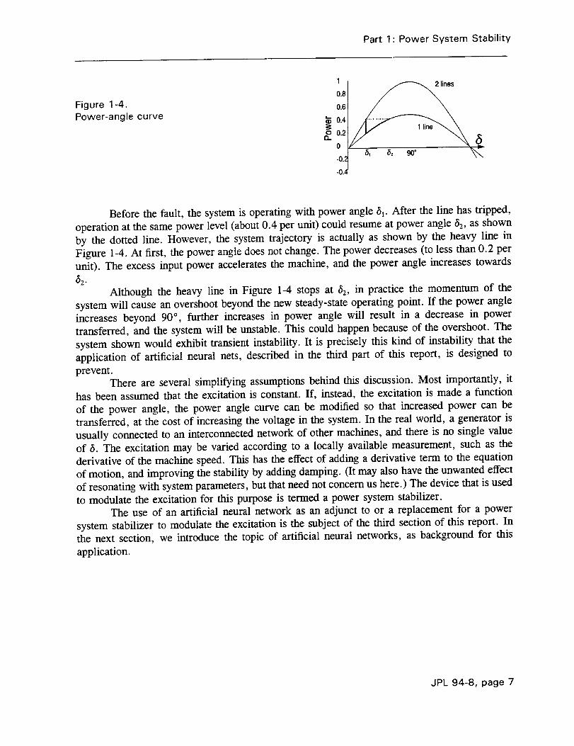
In terms of the power-angle curves, the result is as shown in Figure 1-4.
JPL 94-8, page 6
Part 1: Power System Stability
Figure 1-4.Power-anglecurve
D-
1
0.8
0.6
0.4
0.2
0
.0.2
-0.4
a& _2 90° _.
Before the fault, the system is operating with power angle 3_. After the line has tripped,
operation at the same power level (about 0.4 per unit) could resume at power angle c52,as shown
by the dotted line. However, the system trajectory is actually as shown by the heavy line in
Figure 1-4. At first, the power angle does not change. The power decreases (to less than 0.2 per
unit). The excess input power accelerates the machine, and the power angle increases towards
32.
Although the heavy line in Figure 1-4 stops at 32, in practice the momentum of the
system will cause an overshoot beyond the new steady-state operating point. If the power angle
increases beyond 90 °, further increases in power angle will result in a decrease in power
transferred, and the system will be unstable. This could happen because of the overshoot. The
system shown would exhibit transient instability. It is precisely this kind of instability that the
application of artificial neural nets, described in the third part of this report, is designed to
prevent.
There are several simplifying assumptions behind this discussion. Most importantly, it
has been assumed that the excitation is constant. If, instead, the excitation is made a function
of the power angle, the power angle curve can be modified so that increased power can be
transferred, at the cost of increasing the voltage in the system. In the real world, a generator is
usually connected to an interconnected network of other machines, and there is no single value
of 3. The excitation may be varied according to a locally available measurement, such as the
derivative of the machine speed. This has the effect of adding a derivative term to the equation
of motion, and improving the stability by adding damping. (It may also have the unwanted effect
of resonating with system parameters, but that need not concern us here.) The device that is used
to modulate the excitation for this purpose is termed a power system stabilizer.
The use of an artificial neural network as an adjunct to or a replacement for a power
system stabilizer to modulate the excitation is the subject of the third section of this report. In
the next section, we introduce the topic of artificial neural networks, as background for this
application.
JPL 94-8, page 7


PART 2" NEURAL NETWORKS
HE QUEST for efficient computational approaches to artificial intelligence (AI) hasundergone a significant evolution in the last few years. Attention has come to focus on the
application of neural learning concepts to some of the many tasks performed by machines. This
must be complemented by some insight into how to combine symbolic reasoning with massively
parallel processing abilities. Computer scientists seek to understand the computational potential
of this emerging technology. They are interested in knowing the fundamental limitations and
capabilities of handling unstructured problems by intelligent machines. Issues such as this are
central to the deeper question of the feasibility of neural learning vis gt vis artificial intelligence.
The focus of this part of the report is narrower; to examine generally the capabilities of
neural network learning. Machine learning in the context of neural networks is examined from
the standpoints of computational complexity and algorithmic information theory.
Not only is the concept of massively parallel neuroprocessing of scientific interest, it is
also of great practical interest. It is changing the nature of information processing and problem
solving. In general, the scientific and engineering community is faced with two basic categories
of problems. First, there are problems that are clearly defined and deterministic and controllable.
These can be handled by computers employing rigorous, precise logic, algorithms, or production
rules. This class deals with structured problems such as sorting, data processing, and automated
assembly in a controlled workspace. Second, there are scenarios such as maintenance of nuclear
plants, undersea mining, battle management, and repair of space satellites that lead to computa-
JPL 94-8, page 9
p_ PAGE, BL.A,e4K r_iOT FILtd[#

Part 2: Neural Networks
tional problems that are inherently ill-posed. Such unstructured problems present situations that
may have received no prior treatment or thought. Decisions need to be made, based on
information that is incomplete, often ambiguous, and plagued with imperfect or inexact knowl-
edge. These cases involve the handling of large sets of competing constraints that can tolerate
"close enough" solutions. The outcome depends on very many inputs and their statistical
variations, and there is not a clear logical method for arriving at the answer. The focus of
artificial intelligence and machine learning has been to understand and engineer systems that can
address such unstructured computational problems.
Engineered intelligent systems, that is expert systems with some embedded reasoning,
such as might be used for autonomous robots and rovers for space applications, behave with
rigidity when compared to their biological counterparts. Biological systems are able to recognize
objects or speech, to manipulate and adapt in an unstructured environment and to learn from
experience. Engineered systems lack common sense knowledge and reasoning, and knowledge
structures for recognizing complex patterns. They fail to recognize their own limitations and are
insensitive to context. They are likely to give incorrect responses to queries that are outside the
domains for which they are programmed. Algorithmic structuring fails to match biological
computational machinery in taking sensory information and acting on it, especially when the
sensors are bombarded by a range of different, and in some cases competing, stimuli. Biological
machinery is capable of providing satisfactory solutions to such ill-structured problems with
remarkable ease and flexibility.
An important part of any development for unstructured computation today is to
understand how unstructured computations are interpreted, organized, and carried out by
biological systems. The latter exhibit a spontaneous emergent ability that enables them to self-
organize and to adapt their structure and function, z
Technical success in emulating some of the fundamental aspects of human intelligence
has been limited. The limitation lies in the differences between the organization and structuring
of knowledge, the dynamics of biological neuronal circuitry and its emulation using symbolic
processing. For example, it has been said that analogy and reminding guide all our thought
patterns, and that being attuned to vague resemblances is the hallmark of intelligence (Hofstader,
1979; Kanal and Tsao, 1986; Linsker, 1986a,b,c; Winograd, 1976). Thus, it would be naive to
expect that logical manipulation of symbolic descriptions is an adequate tool. Furthermore, there
is strong psychophysical evidence that while the beginner learns through rules, the expert
discards such rules, somehow instead discriminating thousands of patterns, acquired through
experience in his domain of expertise.
It is rapidly becoming evident that many of the unstructured problems can be solved not
2 A comment about the use of the word emergent is in order. The first dictionary definition is usually
emerging, which doesn't help much. Suddenly appearing and arising unexpectedly are lower in the list
of meanings. Almost certainly, the use of emergent in our context derives from the emergent theory ofevolution which holds that completely new organisms or modes of behavior appear during the process
of evolution as a result of unpredictable rearrangements of pre-existing elements. This use carries with
it the notion that the results do not arise from a higher external control, but from the operation of a form
of natural selection. In nature, the process occurs as a result of feedback, strengthening some (biological)neural connections and weakening others during learning. In our application, the natural selectioncorresponds to the adjustment of the weights during the training of the artificial neural network.
JPL 94-8, page 10

Part 2: Neural Networks
with traditional AI techniques, but by "analogy", "subsymbolic" or pattern matching techniques.
Hence, the neural network, a biologically inspired computational and information processing
approach, provides us with an inherently better tool. In the remainder of this report, we present
tutorial material that will function as a background for further work on the application of
artificial neural networks to power system problems. The remainder of this section of the report
concentrates on neural networks. Their application to the control problems of power system
stability is examined in Part 3. A mathematical formalism that can provide an enabling basis for
solving complex problems is reserved for an Appendix.
The problem of interest here is one that has been addressed for the last several decades,
namely, functional synthesis. Specifically, we focus on learning nonlinear mappings to abstract
functional, statistical, logical and spatial invariants from representative examples. However,
before we formally introduce neural networks in the technical core of this report, we present
arguments comparing the suitability of neural networks and formal AI to solving problems in
computational learning.
AI Modeling and Neural Networks
Over the last three decades, AI and neural network researchers have charted the ground in the
areas of pattern recognition, adaptive machine learning, perception and sensory-motor control.
This has provided an assessment of what is difficult and what is easy. Although both disciplines
have similar goals, there is not much overlap between their projected capabilities. The basis of
both approaches may be traced back to hypotheses of Leibniz (1951) and Weiner (1948). They
identified humans as complicated goal-seeking machines, each composed of an "intelligent" brain
and highly redundant motor systems. This machine can detect errors, change course, and adapt
its behavior so that the achievement of goals is more efficient.
Later development of intelligent systems has pursued two distinct schools of thought;
symbolic and neurobiological, or connectionist. AI researchers concentrated on what the brain
did irrespective of how it was accomplished biologically, while the connectionists focussed on
how the brain worked. The following material is written by a connectionist.
Rooted in the "rationalist, reductionist tradition in philosophy," AI assumes there is a
fundamental underlying formal representation and logic that mirrors all primitive objects, actions
and relations. This view of the world has the necessary and sufficient means for general
intelligent action. Newell and Simon (1976), are the most forceful proponents of this approach.
They hypothesized that if such a representation were available, the operations of human
cybernetic machinery could be fully automated and described by mathematical theorems and
formal logic. They believed all knowledge could be formulated into rules. Hence, behavioral
aspects of human reasoning and perception could be emulated by following rules or manipulating
symbols, without regard to the varying interpretations of symbols. Further, in this view, intel-
ligent behavior arises from the amalgamation of symbols in patterns that were not anticipated
when the rules were written. Expert systems are the product of such a line of investigation.
However, as discussed by Reeke and Edelman (in Graubard, 1989), over the years AI
researchers have struggled against fundamental systems engineering issues summarized as
follows :
JPL 94-8, page 11

Part 2: NeuralNetworks
Coding Problem: finding the suitable universal symbol system, ie the ultimate simple
units by which all complex things can be understood;
Category Problem: specifying a sufficient set of rules to define all possible categories and
phenomena that the system might have to recognize;
Procedure Problem: specifying in advance all actions that must be taken for all possible
combinations of input;
Homunculus Problem: This pins the fundamental problem of AI to the old puzzle of
"infinite regress" in a universal symbol system. For example, when a person looks at an
object, say a computer, how is the image of the computer registered in the brain? All
explanations hitherto proposed by AI attribute this process to some "intelligent device"
inside the brain that is in charge of doing the registering. However, the same problem
has to be faced again to explain how the "device" does the registering, and so on ad
infinitum;
Developmental Problem: devising mechanisms that can enable programmed systems to
exist, self-learn, self-organize their structure and function, and self-replicate without
explicit external manipulation, akin to adaptive biological systems;
Nonmonotonic Reasoning Problem: designing rules that can function as retractable
hypotheses, to mitigate the problems that arise when rules get executed without context-
consistency checks.
Since formal AI has not been able to surmount the above problems using logical
reasoning alone, some have suggested recourse to an alternate scientific paradigm--neural
networks. In a radical philosophical departure from AI, the neural network community argues
that logical reasoning is not the foundation on which cognition is based. Instead, cognition is an
emergent behavior that results from observing a sufficient number of regularities in the world 3.
The theoretical underpinnings of this approach lie in biological detail and rigorous mathematical
disciplines such as the theory of dynamical systems and statistical physics. Neural network
theorists attempt to discover and validate the principles that make intelligence possible by
observing existing intelligent systems, ie the brain. They hold the view that cognitive machinery
is built from many simple, nonlinear, interacting elements. These neural networks store
knowledge in their internal states and self-organize in response to their environments. Intelligentbehavior results from collective interactions of these units.
Historically, the symbolic community has treated the human brain as a hierarchical
system of components which obey the laws of physics and chemistry. The system could be
described as one which generates solutions to mathematical equations by deriving computable
functions from the inputs and outputs of neurons. It is assumed that given an initial state and a
3 One might assume from the origin of the word that the emergent behavior is spontaneous in origin,
and indeed this is the case. The inner workings of most networks defy exact comprehension. One shouldnot, however, be too uncomfortable with this. Artificial neural networks are trained, and while the details
of how that training actually functions cannot be precisely predicted, the overall result can be estimated
satisfactorily.
JPL 94-8, page 12

Part 2: Neural Networks
sufficient amount of computing power, one could compute a person's next state. This approach
ignored the framework of interpretation, "context-sensitivity," within which humans processinformation, make commitments and assume responsibility. The primary focus of AI became to
design rule-systems that processed symbols without regard to their meanings. Thus, it completely
ignored the considerable amount of subsymbolic or subconscious processing that precedes our
conscious decision making, and later leads to the filtering of situations so that the appropriate
rule may be used. In sharp contrast, rather than creating logical problem-solving procedures,
neural network researchers use only an informal understanding of the desired behavior to
construct computational architectures that can address the problem. This, it is hoped, willeliminate the fundamental M limitation, lack of context sensitivity.
Whereas formal AI focusses on symbols, symbolic manipulation, or formal logic proce-
dures, neural networks focus on association, units and patterns of activation. Neurocomputation
primarily entails recognizing statistically emergent patterns, and processing alternatives obtained
by relaxing various features that characterize a situation.
Therein lies the performance potential of neural networks. They are amenable to the
development and application of human-made systems that can emulate neuronal information
processing operations. Examples of applications include real-time high-performance pattern
recognition, knowledge-processing for inexact knowledge domains, and precise sensory-motorcontrol of robotic effectors. These are areas that computers and AI machines are not suited for.
Neural networks are ideally suited for tasks where a holistic overview is required, eg to abstract
relatively small amounts of significant information from large data streams, such as in speech
recognition or language identification. On the other hand, digital computers and AI are ideal for
algorithmic, symbolic, logical and high precision numeric operations that neural networks are
not suited for. The two fields complement each other in that they approach the same problems
but from different perspectives.So far, we have tried to describe the application and potential of neural networks. We
now present a brief summary of their evolutionary history.
A History of Artificial Neural Networks
The field of artificial neural networks has been revitalized by recent advances in the following
three areas:
1. our understanding of anatomical and functional architecture; the chemical composition,
electrical and organizational processes occurring in the brain and nervous system;
2. hardware technology and capability, leading to physical realizations of neural networks;
3. new network architectures with collective computational properties such as time sequence
retention, error correction and noise elimination, recognition, and generalization.
Development of detailed models of neural networks began with the work of McCulloch
and Pitts (1943). Using logical elements they demonstrated that synchronous neural nets could
perform all quantifiable processes, eg arithmetic, classification, and application of logical rules.
Hebb (1949) demonstrated that repeated activation of one group of neurons by another through
a particular synapse leads it to activate synchronously groups of neurons to which it is weakly
JPL 94-8, page 13

Part 2: Neural Networks
connected, thereby organizing strongly connected assemblies. Neumann (in Grossberg 1987b),
injected the notion of redundancy in neurocomputing. He constructed networks which activated
many neurons to do the job of one. Winograd and Cowan (1963), extended his work to introduce
the notion of distributed representation. In this representation, each neuron partially represented
many bits. The field was put on a firm mathematical basis by Rosenblatt (1962). He conjectured
that intelligent behavior based on a physical representation was likely to be difficult to formalize.
According to his arguments, it was easier to make assumptions about a physical system and then
investigate the system analytically to determine its behavior, than to describe the behavior and
then design a physical system by techniques of logical synthesis. He engineered his ideas in a
feedforward network of McCulloch and Pitts neurons (1943), named perceptrons. He attempted
to automate the procedure by which his network of neurons learned to discriminate patterns and
respond appropriately. A detailed study of perceptrons led Minsky and Papert (1969) to strong
criticism of the field. Thereafter, neural network receded into a long slump. However, as
observed by Ladd (1985), Minsky was mistaken in interpreting or suggesting that simple
perceptrons were at the heart of connectionism. Their analysis was not valid for systems that
were more complex, including multilayered perceptrons and neurons with feedback.
The resurgence of the field is due to the more recent theoretical contributions by Kohonen
(1977-1987), Grossberg (1987a, 1987b), Amari (1972-1983), Carpenter and Grossberg (1987a,
1987b), Hopfield ( 1982,1984), and Zak (1988-1991). Hopfield's illuminating contributions have
extended the applicability of neural network techniques to the solution of complex combinatorial
optimization problems (Hop field and Tank 1985).
As shown in Fig. 2-1, artificial neural systems may be characterized as distributed
computational systems comprised of many processing units. Each processing element has
connected to it several others in a directed graph of some configuration. They have been defined
(Kohonen, 1988) as
massively parallel, adaptive dynamical systems modeled on the general features ofbiological networks, that can carry out useful information processing by their state
response to initial or continuous input. Such neural systems interact with the objects of
the real world and its statistical characteristics in the same way as biological systems do.
Figure 2-1.Model of a neural system
BASIC ELEMENT
I i
For the hth neuron
[
//: :, ........ ,
i:iiii ::il
U i is the potential, _ activity level
Wii is the synaplJcweight o! Ire connection from
G i' is the firing rate funclJon
I i is the extemal input
K i is a decay constant
itoj
JPL 94-8, page 14

Part 2: Neural Networks
Grossberg (1988) has observed that neural networks must:
(a) be nonlinear
(b) be nonlocal, ie exhibit long-range interactions across a network of locations
(c) be nonstationary, ie interactions are reverberative or iterative
(d) have nonconvex "energy-like" function.
The potential advantages of neuronal processing arise as a result of the network's ability
to perform massively parallel, asynchronous and distributed information processing. Neurons
with simple properties, interacting according to relatively simple rules, can collectively
accomplish complex functions.Neural network modeling is a discipline which attempts to understand brain-like
computational systems. It has been variously termed computational neuroscience, parallel
distributed processing, and connectionism.The bulk of neural network models can be classified into two categories: those that are
intended as computational models of biological nervous systems or neuro-biological models, and
those that are intended as biologically-inspired models of computational devices with
technological applications, called Artificial Neural Systems (ANS).
Although our primary emphasis is on ANS, we will highlight the influence of neurobiolo-
gy on the formulation of ANS models, and the resulting computational implications. To get a
sense of the required size and interconnectivity of neuronal circuitry for intelligent behavior, we
begin by examining biological neural networks. Most existing neural network models are basedon idealizations of the biological neuron and the synaptic conduction mechanisms, shown in
Figure 2-2.
_ CYTON
//
AXON
Figure 2-2. ..... NUCLEUSBiological neuron
DENDRITES AXON TERMINALS
As shown in Fig 2-2, each neuron is characterized by a cell body or cyton and thin branching
extensions called dendrites, that are axons specialized for inter-neuron transmission. The dendrite
is a passive receiving and transmitting agent, whereas the axon is electrochemically charged, a
highly active brain cell entity. The dendrites receive inputs from other neurons (by way of
chemical neurotransmitters), and the axon provides outputs to other neurons. The neuron itself
is imbedded in an aqueous solution of ions, and its selective permeability to these ions (the cell
membrane contains ion channels) establishes a potential gradient responsible for transmitting
information. The electrochemical input signals or the neurotransmitter is funneled to the neuron
from other neurons, to which it is connected through sites on the their surface, called synapses.
The input signals are combined in various ways, triggering the generation of an output
signal by a special region near the cell body. However, the neurobiological phenomenon that is
of particular interest is the changing chemistry of the synapse as information flows from one
JPL 94-8, page 15

Part 2: NeuralNetworks
neuron to another. The synapse instantaneously decides when the information is not essential and
need not be resupplied. The weight of the individual charge is regarded as the determining
factor. On the transmitting or pre-synaptic side of the synapse, triggering of the synaptic pulse
releases a neurotransmitter that diffuses across a gap to the receiving side of the synapse. On
the post-synaptic or receiving side, the neurotransmitter binds itself to receptor molecules,
thereby affecting the ionic channels and changing the electrochemical potential.
The magnitude of this change is determined by many factors local to the synapse, eg the
amount of neurotransmitter released, and the number of post-synaptic receptors. Therefore,
neurocomputation, biological self-organization, adaptive learning and other mental
phenomena are largely manifested in changes in the effectiveness or "strength" of the
synapses, and their topology. Additional details on the biological neuron, membrane polar-
ization chemistry and synaptic modification may be found in Aleksander (1989).
The above insights in neurobiology have led to the mathematical formulation of simulated
neurons, ie the basic building block of neural network models. A functional model for a typical
simulated neuron is shown in Figure 2-3.EXCITORY
INPUTS_._x_EGRATOR
Figure 2-3. _UTPtrrFunctional model of simulated neuron
INHIBITORYINPUTS
WEIGHTING FACTORS1 THRESHOLD
. "_ OUTPUT
' -' I/_ SUMMER
Four useful areas may be abstracted. The first is the synapse where signals are passed from one
neuron to another, and the amount of signal is regulated, ie gated or weighted by the strength
of the synaptic interconnection. In the activated neuron region, called the summer, synaptic
signals containing excitatory and inhibitory information are combined. This affects the tendency
of a cell to fire or not. The threshold detector actually determines if the neuron is going to fire
or not. The axonal paths conduct the output activation energy to other synapses to which theneuron is connected.
Useful properties such as generalization, classification, association, error correction, and
time sequence retention emerge as collective properties of systems comprised of aggregations
of many such simple units. When viewed individually, the dynamics of each neuron bears little
resemblance to task being performed.
As discussed in the preceding paragraph, of particular computational and modeling
interest are the mathematical notions of synapse and synaptic modification. Further attention is
paid to mechanisms by which such units can be connected together to compute, and the rules
whereby such interconnected systems could be made to learn.
Computational Neural Learning
The strength of neural networks for potential applications arises from their spontaneous
(emergent) ability to achieve functional synthesis. That is to say, they learn nonlinear mappings,
and abstract the spatial, functional or temporal invariances of these mappings. Relationships
between multiple inputs and outputs can be established, based on a presentation of many
JPL 94-8, page 16
Part 2: NeuralNetworks
representative examples. Once the underlying invariances have been learned and encoded in the
topology and strengths of the synaptic interconnections, the neural network can generalize to
solve arbitrary problem instances. Applications which require solving intractable computational
problems or adaptive modeling are of special interest.
Neural Learning has been defined as the process of adaptively evolving the internal
parameters, eg connection weights and network topology, in response to stimuli (representative
examples) being presented at the input (and possibly at the output) buffer. Neural networks
modeled as adaptive dynamical systems rely on relaxation methods rather than a heuristic
approach for automatic learning.
Learning in neural networks may be supervised. In this case, the desired output response
to the input stimuli patterns is obtained from a knowledgeable teacher. The network is presented
repeatedly with training patterns, and detects the statistical regularities embedded within them.
It learns to exploit these regularities to draw conclusions when presented with a portion or a
distorted version of the original pattern. The retrieval process involves presentation of one of
the stimuli patterns to the network and comparison of the network response to the desired one.
When a portion of a training pattern is used as a retrieval cue, the learned process is called auto-
associative. When the presented input is different from any input presented during training, the
learning is called hetero-associative.
When no desired output is shown to the network the learning is unsupervised. This kind
of learning is relevant to grouping or clustering. For instance, let us assume that the network
is presented with 10 different pictures of two different individuals. After training, the network
will have three states, ie, individual A, B or not known. When the network is presented with
one of the ten pictures, or one sufficiently close to one of them, it should converge to A or B.
On the other hand, presenting a totally new picture to the network may result in convergence
to any of the three states. However, to train the network on labeling the states is a task for
supervised learning.
An intermediate kind of learning is reinforcement learning. Here, a teacher indicates
whether the response to an input is good or bad, how far and in what direction the output differs
from the desired output. The network is rewarded or penalized depending on the action it takes
in response to each presented stimulus. The network configures itself to maximize the reward
that it receives. To illustrate the point, let us take the analogy of a driver trying to park a car
with the assistance of an outside person. In this case, the assistant, playing the role of the
teacher, will give only directions such as, left, more to the left, straight, etc. The teacher does
not have the means to give quantitative value such as 20 degrees to the right. Once the training
is done, the driver should be able to park the car without any assistant.
Along with the architecture, learning rules form the basis of categorizing different neural
network models. A detailed description of different types of learning rules can be found in
Lippmann (1987). Neural learning rules could take the following forms:
Correlational Learning, where parameter changes occur on the basis of local or global
information available to a single neuron. A good example is the Hebbian learning rule
(Hebb, 1949), in which the connection weights are adjusted according to a correlationbetween the states of two interconnected neurons. If the two neurons were both active
during some successful behavior, the connection would be strengthened to express the
positive correlation between them.
JPL 94-8, page 17
Part 2: NeuralNetworks
On the other hand, in Error-corrected Learning, the rules work by comparing the
response to a given input pattern with the desired response. Weights modifications are
calculated in the direction of decreasing error. Examples are the perceptron learning rule,
and back-propagation. In this category, two methods are available for updating the
weights: (a) add up the weight change due to all stimuli patterns and make an average,
or (b) apply the weight changes due to each stimulus as they are computed. In principle,the two methods should converge into the same end results. However, simulation results
indicate that the first approach is faster.
Another learning rule, Reinforcement Learning, does not require a measure of the desired
responses, either at the level of a single neuron or at the level of a network. A measure
of the adequacy of the emitted response suffices. This reinforcement measure is used to
guide the search process to maximize reward.
Another category is Stochastic Learning, where the network's neurons influence each
other through stochastic relaxation, eg, Boltzmann Machine. In this method, learning
takes place in two stages. First, the network is run with both the input and output
neurons clamped (ie, the value of the input and output neurons set to desired values). Co-
occurrency probabilities are calculated after the network has reached a global minimum.
This procedure is repeated with only the input neurons clamped. Synaptic weights arethen adjusted according to gradient-descent direction.
Two important parameters that characterize the computational power of neural learning
formalisms are the nature of the states of individual neurons, and the temporal nature of synaptic
updating. The states of individual neurons may be either discrete or continuous. It has been
shown that a network with a finite number of states is computationaUy equivalent to a finite statemachine.
Further, the nature of the time variable in neural computation may also be either discrete
or continuous. In the discrete case, the dynamics can be modeled by difference approximations
to differential equations. It has been shown that continuous time networks can resolve temporal
behavior which is transparent in networks operating in discrete time. In all respects, the two
classes are computationally equivalent.
Adaptive Neural Control System Architectures
In a fundamental sense, the control design problem is to find an appropriate functional mapping,
from measured and desired plant outputs, to a control action that will produce satisfactory
behavior in the closed-loop system. In other words, the problem is to choose a function (a
control law) that achieves certain performance objectives when applied to the open-loop system.
In turn, the solution to this problem may involve other mappings, eg from the current plant
operating condition to the parameters of a controller or local plant model, or from measured
plant outputs to estimated plant state. Accordingly, a learning system that could be used to
synthesize such mappings on-line would be an advantageous component of an intelligent control
system. To successfully employ learning systems in this manner, one must have an effective
means for their implementation and incorporation into the overall control system architecture.
JPL 94-8, page 18

Part 2: NeuralNetworks
Neurocontrol is defined as the use of well-specified neural networks to emit actual control
signals. In the last few years, hundreds of papers have been published on neurocontrol, but
virtually all of them are still based on five basic design approaches:
. Supervised control, where neural nets are trained on a database that contains the
"correct" control signals to use in sample situations;
. Direct inverse control, where neural nets directly learn the mapping from desired
trajectories to the control signals which yield these trajectories;
. Neural adaptive control, where neural nets are used instead of linear mappings in
standard adaptive control;
. The backpropagation of performance, which maximizes some measure of performance
over time, but cannot efficiently account for noise and cannot provide real-time learning
for very large problems;
. Adaptive critic methods, which may be defined as methods that approximate dynamic
programming (ie, approximate optimal control over time in noisy, nonlinear environ-
ments).
Based upon preliminary studies, it is clear that methods 1, 2, and 4 are not well suited
to solve the problem at hand. At this stage, it also seems that both methods 3 and 5 are capable
of solving the problem. However, an in-depth study is needed to demonstrate the superiority of
one over the other. Since the neural adaptive control methodology has the advantage of being
implemented in a straightforward manner, ie as an add-on to the existing adaptive controller, its
implementation and performance will be investigated and analyzed first.
Having discussed the basic features of neural learning systems for control, we will briefly
describe hybrid control system architectures that exhibit both adaptive and learning behaviors.
These hybrid structures incorporate adaptation and learning in a synergistic manner. In such
schemes, an adaptive system is coupled with a neural learning system to provide real-time
adaptation to novel situations and time-varying dynamics. The adaptive control system reacts to
discrepancies between the desired and observed behaviors of the plant, to maintain the requisite
closed-loop system performance. These discrepancies may arise from time-varying dynamics,
disturbances or unmodeled dynamics. The phenomena of time-varying dynamics and disturbances
are usually handled through feedback in the adaptive system. In contrast, the effects of some
unmodeled dynamics can be predicted from previous experience. This is the task given to the
learning system. Initially, all unmodeled behavior is handled by the adaptive system; eventually
however, the learning system is able to anticipate previously experienced, yet initially
unmodeled behavior. Thus, the adaptive system can concentrate on novel situations (where little
or no learning has occurred) and time-varying behavior.
In the following, two general hybrid architectures are outlined. The discussion of these
architectures parallels the usual presentation of direct and indirect adaptive control strategies.
In each approach, the learning system is used to alleviate the burden on the adaptive controller
of continually reacting to predictable state-space dependencies in the dynamical behavior of the
plant. Note that various technical issues must be addressed to guarantee the successful
implementation of these approaches. For example, to ensure both the stability and robustness of
the closed-loop system (which includes both the adaptive and learning systems, as well as the
JPL 94-8, page 19

Part 2: Neural Networks
plant), one must address issues related to controllability and observability; the effects of noise,
disturbances, model-order errors, and other uncertainties; parameter convergence, sufficiency
of excitation, and nonstationarity; computational requirements, time-delays, and the effects of
finite precision arithmetic. Many (if not all) of these issues arise in the implementation of
traditional adaptive control systems; as such, there are some existing sources one may refer to
in the hope of addressing these issues. Although these topics are well beyond the scope of this
document, in some instances, the learning-augmented approach appears to offer operational
advantages over the corresponding adaptive approach (with respect to such implementation
issues). For example, a typical adaptive system would require persistent excitation to ensure the
generation of accurate control or model parameters, under varying plant-operating conditions.
A learning system, however, would only require sufficient excitation, during some training
phase, to allow the stationary, state-space dependencies of the parameters to be captured.
Direct Implementation
In the typical direct adaptive control approach, see Figure 2-4, each control action u is generated
based on the measured Ym and desired ya plant outputs, internal state of the controller, and
estimates of the pertinent control law parameters k. The estimates of the control law parameters
are adjusted, at each time-step, based on the error e between the measured plant outputs and the
outputs of a reference system y,. Of course, care must be taken to ensure that the plant is
actually capable of attaining the performance specified by the selected reference system. Direct
adaptive control approaches do not rely upon an explicit plant model, and thus avoid the needto perform on-line system identification.
Figure 2-4.Direct adaptive control
Yd
The controller in Figure 2-4 is structured so that normal adaptive operation would result if the
learning system were not implemented. The reference represents the desired behavior for the
augmented plant (controller plus plant), while the adaptive mechanism is used to transform the
JPL 94-8, page 20

Part 2: Neural Networks
reference error directly into a correction, zik for the current control system parameters. The
adaptation algorithm can be developed and implemented in several different ways (eg, via
gradient or Lyapunov-based techniques. Learning augmentation can be accomplished by using
the learning system to store the required control system parameters as a function of the operating
condition of the plant. Alternatively, learning can be used to store the appropriate control action
as a function of the actual and desired plant outputs. The schematic architecture in Figure 2-4shows the first case.
When the learning system is used to store the control system parameters as a function of
the plant operating condition, the adaptive system would provide any required perturbation to
the control parameters k generated by the learning system. The signal from the control block
to the learning system in Figure 2-4 is the perturbation in the control parameters 6k to be
associated with the previous operating condition. This association (incremental learning) process
is used to combine the estimate from the adaptive system with the control parameters that have
already been learned for that operating condition. At each sampling instant, the learning system
generates an estimate of the control system parameters k associated with that operating
condition, and then passes this estimate to the controller, where it is combined with the
perturbation parameter estimates maintained by the adaptive system and used to generate the
control action u. In the ideal limit where perfect learning has occurred, and there is an absence
of noise, disturbances, and time-varying dynamics, the correct parameter values would always
be supplied by the learning system, so that both the perturbations 6k and corrections zlk
generated by the adaptive system would become zero. Under more realistic assumptions, there
would be some small degradation in performance because of adaptation (eg, tSk and zik might
not be zero because of noise).
In the case where the learning system is trained to store control action directly as a
function of the actual and desired operating conditions of the plant, the adaptive system would
provide any required perturbation to the control action generated by the learning system. Note
that a dynamic mapping would have to be synthesized by the learning system if a dynamic
feedback law were desired (which was not necessary in the first case). The advantage of this
approach over the previous one is that a more general control law can be learned. The
disadvantage is that additional memory is required and that a more difficult learning problemmust be addressed.
Indirect Implementation
In the typical indirect adaptive control approach, see Figure 2-5, each control action u is
generated based on the measured Ym and Ya desired plant outputs, internal state of the controller,
and estimated parameters Pa of a local plant model. The parameters k for a local control law are
explicitly designed on-line, based on the observed plant behavior. If the behavior of the plant
changes (eg, because of nonlinearity), an estimator automatically updates its model of the plant
as quickly as possible, based on the information available from the (generally noisy) output
measurements. The indirect approach has the important advantage that powerful design methods
(including optimal control techniques) may potentially be used on-line. Note, however, that
computational requirements are usually greater for indirect approaches, since both model
identification and control law design are performed on-line.
JPL 94-8, page 21
Part2: Neural Networks
Figure 2-5.Indirect adaptive control
klICONT.OLI
I=_NIN_:
Ym
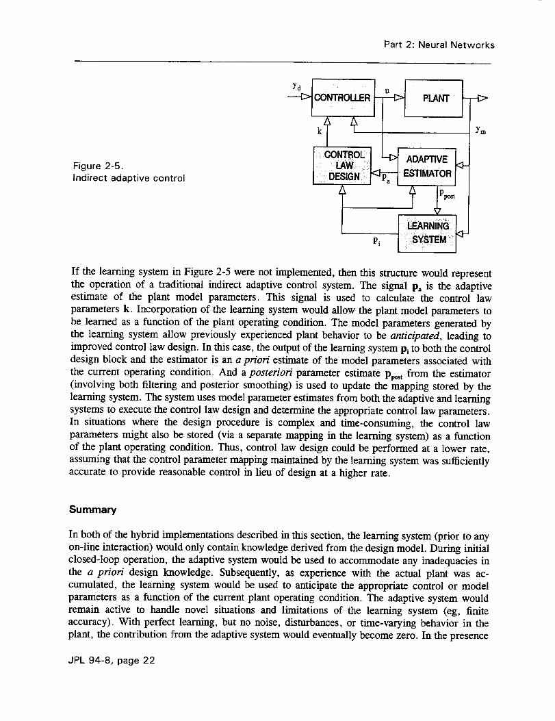
If the learning system in Figure 2-5 were not implemented, then this structure would represent
the operation of a traditional indirect adaptive control system. The signal p= is the adaptiveestimate of the plant model parameters. This signal is used to calculate the control law
parameters k. Incorporation of the learning system would allow the plant model parameters to
be learned as a function of the plant operating condition. The model parameters generated by
the learning system allow previously experienced plant behavior to be anticipated, leading to
improved control law design. In this case, the output of the learning system Pl to both the control
design block and the estimator is an a priori estimate of the model parameters associated with
the current operating condition. And a posteriori parameter estimate Pp_t from the estimator
(involving both filtering and posterior smoothing) is used to update the mapping stored by the
learning system. The system uses model parameter estimates from both the adaptive and learning
systems to execute the control law design and determine the appropriate control law parameters.
In situations where the design procedure is complex and time-consuming, the control law
parameters might also be stored (via a separate mapping in the learning system) as a function
of the plant operating condition. Thus, control law design could be performed at a lower rate,
assuming that the control parameter mapping maintained by the learning system was sufficiently
accurate to provide reasonable control in lieu of design at a higher rate.
Summary
In both of the hybrid implementations described in this section, the learning system (prior to any
on-line interaction) would only contain knowledge derived from the design model. During initial
closed-loop operation, the adaptive system would be used to accommodate any inadequacies in
the a priori design knowledge. Subsequently, as experience with the actual plant was ac-
cumulated, the learning system would be used to anticipate the appropriate control or model
parameters as a function of the current plant operating condition. The adaptive system would
remain active to handle novel situations and limitations of the learning system (eg, finite
accuracy). With perfect learning, but no noise, disturbances, or time-varying behavior in the
plant, the contribution from the adaptive system would eventually become zero. In the presence
JPL 94-8, page 22

Part 2: NeuralNetworks
of noise and disturbances, the contribution from the adaptive system would become small, but
nonzero, depending on the hybrid scheme used. However, the effect of this contribution might
be negligible. In the general case involving all of these effects, the hybrid control system should
perform better than either subsystem individually. It can be seen that adaptation and leaming are
complementary behaviors, and that they can be used simultaneously (for purposes of automatic
control) in a synergistic fashion.
Neural Hardware Implementation
Even to date, a majority of the work in the field of artificial neural networks consists of theory,
modeling, and software simulations of the massively parallel architectures on conventional digital
computers. However, to realize the promise of a high speed, inherently parallel neural network,
architectures must be implemented in parallel hardware. This way, many neurons can actually
communicate and orchestrate their activities simultaneously.
The basic components of electronic neural net hardware are conceptually and functionally
extremely simple. The neurons can be implemented as thresholding nonlinear amplifiers and the
synapses as variable resistive connections between them. An artificial neural network therefore,
consists of many simple processing elements, representing neurons, which interact among
themselves through networks of weighted connections functioning as synapses. The computation
performed by the network is determined by the synaptic weights or connection strengths. The
state of the system is identified by the pattern of activity of the neurons. Given an initial activity
pattern, each neuron receives input signals from the neurons and adjusts its output accordingly
over time. The system rapidly evolves into steady activity pattern which is then interpreted as
a memory recall or as a solution to a problem.
As might be expected, the field of neural networks has developed its own computational
terms. Some understanding of these terms is necessary to appreciate neural network simulation
and implementation requirements. Some of the key concepts and terms are:
A typical neural network contains many more interconnects than neurons, or processingelements.
• Each interconnect requires one multiply/accumulate operation for summing.
Digital computers are normally assessed in terms of storage or memory (where the unit
of measure is words) and speed (instructions-per-second or floating-point-operations-per-
second). The field of neural network defines storage as the value of the input weights and
measures it by the interconnects-per-second within a layer or between layers. (This way
of conceiving neural network storage is important only in the case of network simulation;
in the case of implementation in special-purpose hardware, storage would be handled by
resistive networks and would be defined differently.)
To understand this vernacular and its implications, we will use the terms interconnects
and interconnects-per-second to chart a set of coordinates. We will place interconnects on the
horizontal axis and interconnects-per-second on the vertical axis, respectively. The environment
defined by this chart will be used to describe the computational capabilities of neural network
systems and applications.
JPL 94-8, page 23

Part 2: Neural Networks
To fix the idea, let us introduce the computational capabilities of certain biological
systems, as can be seen in Figure 2-6.
t_
==oo
.=_v
¢-_LIIWO.Ct)
Figure 2-6.Computational capabilitiesof some biological systems
10_6-
10t 4-
1012 -
aplysia•101°
• fly108
106
. leech • worm
104102 ii, lO4 '106 ' 10' 1()1°
STORAGE (interconnects)
human•
10TM 1()14
• bee• cockroach
A human, with the staggering capacity of 1014 interconnects and 1016 interconnects per second,
can be viewed as a superpower compared to creatures such as the worm, the fly, and the bee.
In this context, neural network researchers would be very pleased to be able to replicate the
computational capabilities of a fly or a bee with a machine. However, that will be difficult with
the tools presently available. Today's neural network researchers have access to a variety of
digital tools, that range from low-priced microprocessor-based workstations, through attached
processors and bus-oriented processors, to the more expensive massively-parallel machines, and
finally to supercomputers.
Generally, the micro/minicomputers provide a very modest interconnects-per-second
capability, though in some cases storage capacity is substantial. The speed of these devices is
limiting; neural network models take a very long time to run on them. Attached processors
improve this situation somewhat, since they can boost interconnects-per-second into the millions
from the hundreds of thousands. Bus-oriented processors, in some cases, raise by an order of
magnitude the number of interconnects-per-second available, but storage is not equivalently
greater. The massively parallel systems feature no better speed, and there remain gaps between
their speed and storage capabilities. Supercomputers, meanwhile, do not offer significantly more
capability than systems which cost far less. In addition, the programming necessary to run neural
network models on these massively parallel machines is very complex. It is, in fact, a problem
which limits the extent to which these systems can be used to conduct neural network research.
Moreover, the architectural limitations of these systems prevent researchers from stacking up
several of them to significantly boost their storage or speed.
The present state of neural hardware, in the context of interconnects (storage) and
interconnects-per-second (speed), may satisfy small size simulations. However, it is not very
user-friendly for research, statistical work, or development of large databases. Nevertheless,
several technologies are poised to push hardware capabilities beyond their present speed and
storage limits:
Gallium arsenide (GaAs) and special-purpose charge-coupled devices (CCDs) will push
up the ceiling on interconnects-per-second.
JPL 94-8, page 24

Part2: Neural Networks
Continued developments in random-access memory (RAM) technology as well as the
lesser-developed three-dimensional (3-D) chip technology are expected to expand current
storage capacities.
Multiprocessing, meanwhile, will allow the boundaries of simulation to be moved upward
by an order of magnitude.
Certainly, if neural networks are to offer solutions to important problems, those solutions
must be implemented in a form that exploits the physical advantages offered by neural networks.
The advantages include high throughput that results from massive parallelism (realtime
operation), small size, and low power consumption. In the near term, smaller neural networks
may be digitally implemented using conventional integrated circuit techniques. However, in the
longer term, implementation of neural networks will have to rely on new technologies.
Currently, the development of neural hardware is focussed on the following three major areas:
Direct VLSI/VHSIC (very large scale integration/very high speed integrated circuits). A
mature technology limited to a low density of interconnects due to its two-dimensional
nature. All the weights in a neural network implemented in direct VLSI/VHSIC would
have to be stored in memory, which would require a lot of capacity.
Analog VLSI, which holds promise for a near-term solution. It is two-dimensional, and
offers a high density of interconnects. This is accomplished because the weights can be
implemented in resistors, thereby obviating the need for additional memory.
Optical technology, less developed and longer-term than the silicon-based approaches and
limited in the types of neural networks that it can implement. This offers a very high
density of interconnects due to its three-dimensional nature.
Table 1 summarizes the state of the art neural hardware currently available or under
development. New chips such as these are needed, not only to build neural network simulators,
but also because they may become very valuable individually in neural network-based
applications.
The fabrication and investigation of neural network architectures with different levels of
complexity and various sizes is currently the subject of research. Our approach here at JPL
involves development of fully parallel, cascadable "building blocks". This effort has already
resulted in neural hardware such as fully programmable synaptic interconnection arrays and
nonlinear analog (variable gain sigmoid) neuron arrays. The modular building blocks have served
very well as flexible and versatile research tools. These tools have been employed in the study
of the emergent properties of neural networks. They also provided a sound baseline and
guidelines for the design and implementation of application-specific, high performance
"neuroprocessors". Such neural hardware has successfully been used for solution of real-life
problems, not only at JPL, but also at several other institutions engaged in neural network
research and development.
JPL 94-8, page 25

Part2: NeuralNetworks
Table 1. Comparisonof architecturesand technologies
System Accuracy Speed Technology(bits) ps/conn
AnalogCMOS
ANNA (AT&T) 6 1 0.9#" CMOSDuong et al (JPL) 6 0.5 2#" CMOSKub et al (NRL) 6 0.5 3#" CMOS
CCDs
Chaing (MIT) 6 0.6 3#" CCDOptoelectronic
Frye et al (AT&T) 6 0.5 Si:HDigital
Uchimuri et al (UNM) 8 0.1 0.8#' CMOSNewell et al (NTT) 8 0.025 1.6#" CMOSCID (Caltech) 6 0.6 2#" CMOS
We have implemented both feedback and feedforward architectures using the cascadable
synaptic and neuron building blocks. The computing speed of such systems exceeds 10 9 analog
operations per second. This is an order of magnitude higher than speeds achievable by neuralnet simulations on sequential machines. Using these networks, we have demonstrated content-
addressable, associative memory, terrain trafticability determination, and solutions to the color
graph optimization and Hopfield-Tank traveling salesman problems. This work is currently
leading to the development of application-specific neuroprocessors.
At JPL, we have successfully demonstrated not only the feasibility of hardware
implementations of neural networks, but also--in spite of the inherent, unavoidable precision
limits and noise constraints--unique strengths of analog processing implemented in parallelhardware.
Conclusions
, Massively parallel information processing schemes, inspired by neural network models,
have become a subject of great interest in recent years. Mathematical modeling and
computer simulations have shown emergent computational properties of complex
networks of neuron-like nonlinear processing elements. These networks capture certain
important aspects of intelligent information processing, not easily dealt with by existing
digital and artificial intelligence (AI) technologies.
. Neural network research has matured greatly, thanks to: (a) development of advanced
mathematical theories and new computer tools, and also (b) a better understanding ofneurobiology.
JPL 94-8, page 26

Part 2: Neural Networks
. Artificial neural networks promise efficient solutions to a variety of problems such as
associative, fault-tolerant, information processing, pattern recognition, control, and
computation intensive global optimization operations. They also provide new capabilities,
such as "learning" from experience in the field, self-organization, and generalization, to
solve ill-posed problems.
. Neural networks are an especially valuable technology when the availability of a good
solution in a very short time is more important than its absolute accuracy.
. To date, a large portion of the work in the field is based primarily on software simulation
of the network architectures on standard sequential computers. Undoubtedly, a simulation
of even a moderately large network, with just a few hundred neurons, becomes a
computation-intensive and time-consuming task on a sequential machine. To realize the
potential speed in artificial, inherently parallel, neural network architectures, the neurons
must process information in parallel.
. Today's computer tools--with simulation capabilities of roughly 10 7 interconnects per
second--fall far short of the computational capabilities of even modest biological
networks; a fly, for instance, computes at 10 9 interconnects per second.
. Under the sponsorship of the Defense Advanced Research Projects Agency (DARPA),
and its successor the Advanced Research Projects Agency (ARPA), JPL has focussed on
the development and demonstration of feasibility of fully parallel neural network
architectures. These are used as high speed research tools to study the emergent
properties of neural networks.
, Neural network technology readiness at JPL has already progressed from feasibility
demonstrations to development and rapid hardware prototyping. Stand-alone application-
specific algorithms and coprocessor systems offering real-time functional capabilities,
previously nonexistent, are now available. These tools offer orders-of-magnitude speed
enhancement in computation intensive problems of interest.
JPL 94-8, page 27


PART 3. APPLICATION
HE OPERATION of an electric power system has two objectives: firstly security, secondlyeconomic operation. First, it is necessary to ensure that there is enough generation and
transmission capacity to meet the load. Then, if there is sufficient capacity, the most efficient
way to meet that load can be sought. System operation can be viewed as controlling a multi-
variable system within the constraints of secure operation. In a multidimensional space
representation, the constraints are the boundaries of the space. The system operates at a point
within (or on the boundary of) the space. More flexibility of operation would result from
expanding the boundaries. Such additional flexibility would allow the freedom to improve
efficiency. The object of the work in neural networks is to facilitate energy efficiency by pushing
against the boundaries of secure operation.
In a power network, power flows will distribute themselves in the system according to
Kirchoff's laws. The self-adjusting nature of the system means that the constraints that represent
safe practice may be violated if part of the system changes (for example, because of a fault).
This topic was reviewed in the first part of this report. The practical result is that the system
must be carefully monitored and controlled.
Human operators, trained and experienced, are adept at operating even complicated
power systems. This is the more impressive when one realizes the complexity and magnitude
of the problem. However, no operator can control a system during a disturbance, or in the
seconds following one. The actions of the operator are limited to ensuring that constraints are
JPL 94-8, page 29
PitlDIk_ PAGE BLANt_ NOT FILP,_E,'3

Part 3: Application
not violated during normal operation, and to restoring as much of the system as possible, after
a fault--and the ensuing actions of the protection system--have changed the system config-
uration. Nor can an operator cope with the swings that some systems experience because of
devices that are installed to make possible the transmission of greater amounts of power over
existing rights of way. The problem will be illustrated by means of the example of power systemstabilizers.
The equations that govern the motion of a power system are second-order and non-linear.
The fact that the equations are second order is of no great import, but the nonlinearity reflects
the fact that the system can become unstable. Consider the system of Figure 3-1.
Figure 3-1.Simple power system
GENERATOR
INFINITE
BUS
For a simple power system, such as the one shown in Figure 3-1, consisting of only one gener-
ator and an infinite bus, the motion is described by the swing equation:
M dz6 + em,_ sin5 =Poutdt 2
where M is the inertia constant, a term related to the angular momentum of the generator, 5 is
the angle between the voltages 1"i and 1,'2 at the generator and the bus, X is the impedance of the
generator, or more generally the impedance across which power is transferred, and Pi, is the
shaft input power.
Several simplifying assumptions have been made, particularly with regard to the
constancy of the parameters. The angular momentum of the generator is a function of the speed.
Clearly this is not constant during a swing. The generator impedance is not constant, either,
since the rotor moves relative to the rotating magnetic field of the stator. It is also assumed that
there is no exciter action, that is, the voltage behind the generator impedance is assumed
constant. (In practice, this voltage is controlled by an AVR, as discussed in Section 1.) Never-
theless, in spite of these assumptions, the swing equation is instructive for the purposes of
illustrating the behavior of the system.
This equation is basically a nonlinear version of the equation that describes the motion
of a pendulum. The oscillations typically have a frequency in the order of a second or so,
determined by the inertia of the generator and the impedance of both the generator and the line
between the generator and the bus. The oscillations are not highly damped (there is no first-order
term, because the resistances have been neglected), and can sometimes lead to instability.
The equation also shows that there is a maximum value to the amount of power that can
be transmitted from the generator to the load. This occurs when 5 reaches 90 °. Any further
increase in the power will result in instability.
In practice, systems with long lines are more prone to instability problems, because of
the relatively large value of the transfer impedance. Some improvement can be made by adding
JPL 94-8, page 30

Part 3: Application
capacitors in series with the line. However, this can affect the ability of the system to maintain
a proper voltage profile, and can sometimes lead to subsynchronous oscillations (ie, oscillations
at frequencies less than power frequency), that can be damaging to generators. The instability
problems are characterized by a frequency in the order of 1 Hz, a frequency which is much too
fast for the generator governor to control. (Governor actuation involves moving a large, slow
valve in the steam or water line driving the turbine.)
To guard against this kind of stability problem, it is possible to modulate the signal at
the AVR controlling the generator exciter. This is done by means of a control system called a
power system stabilizer (PSS). In essence, a PSS functions by adding a derivative term to the
equation of motion. It does this by modulating the exciter in response to changes in the power
system. Power system stabilizers represent a relatively new technology, but one that may have
its roots in some work done by the U.S. Bureau of Reclamation in the late 1960s (Schleif and
White, 1966; Schleif, Hunkins, Hattan and Gish, 1969).
Figure 3-2 shows some of the control systems associated with a generator, including a
power system stabilizer.
{ GOVERNORI- SPEED
Figure 3-2.Generator controls
POWER
bOLT L I EXCITER I /_ VOLTAGE
I &AVR _+ REFERENCE
II I _ SPEED ORSTABILIZER I- FREQUENCY
OR POWER
For the application of a PSS to be successful, it must be "tuned" to the power system, that is,
the parameters of the control system must be adjusted so that the modulation has the desired
effect. Gains and frequency responses must be set to the appropriate values. Typically, a
stabilizer will take the derivative of a speed signal, a process which is inherently noisy. To
remove this noise, it will use a low-pass filter. Tuning thus becomes a problem of adjusting the
lead and lag components of the filter in the stabilizer so that the appropriate correcting signal
is available, without noise.
However, the parameters of the power system are not constant, being subject to daily,
weekly and annual cycles, as well as the changes due to the occurrence and clearing of faults.
PSS settings are rarely correct, therefore, long after the original settings have been made.
They suffer from another defect, too. When there is one machine and an infinite bus, it
is easy to see in which direction the modulation must occur to improve the system stability. This
is not so obvious when the power system becomes more complex. Consider the relatively simple
3-machine system of Figure 3-3.
JPL 94-8, page 31

Part 3: Application
Figure3-3.3-machinepower system
In the Figure, three generators supply load to two buses. (One of the generators has no local
load.) Suppose that a PSS is installed on one of the generators, and that the system is disturbed
in some way. The PSS has been tuned for the situation shown, and will act so as to damp the
swing of the machine to which it is attached. Note that the PSS tuning will not be correct if the
system configuration changes. It is fortunate that PSS tuning is relatively "low Q."
Now suppose that a PSS is added to another generator. Interaction between the two
control systems is inevitable. Just as a swing in one part of the system will affect the other parts
of the system, so an action by a PSS in one part of the network will affect the other parts. This
has not been a significant problem in the past because of the low penetration of PSSs into the
power transmission system. However, power system stabilizers are increasingly likely to be seen
as inexpensive alternatives to system reinforcements. Their impact on the power system will
increase. Before long, PSS interactions will be a problem.
Application of Neural Networks
Artificial neural networks mimic the intelligent information processing abilities of the brain. This
is accomplished through a massively parallel architecture containing a number of logic elements
(the biological term is neurons, but the word node is sometimes used), connected to each other
with variable strengths through a large network of interconnections (synapses).
Collectively, neurons with simple properties can accomplish complex functions such as
control, pattern classification, information reconstruction, and learning. Their strength for many
applications arises from their ability to learn and abstract spatial and/or temporal invariances of
mappings. These networks can be built in hardware, or simulated in software.
A solution to the problems of power system stability control based on the use of artificial
neural networks would have wide applicability; as well as being useful as adjuncts to power
system stabilizers, they could be used for control in systems containing dc links, for example,
and systems containing FACTS devices. (FACTS stands for flexible ac transmission system. The
flexibility comes from the use of devices based on solid state switching to control the apparent
value of system parameters by changing the relationship between voltage and current.)
Implemented as an adjunct to a power system stabilizer, a neural net solution might be
as shown in Figure 3-4. Other forms of implementation are possible. In Figure 3-4 the neural
network is essentially an add-on to the stabilizer. In a fully developed system, there may be no
need for the stabilizer to exist separately from the neural network. All the functions of the
stabilizer could be implemented in the network.
JPL 94-8, page 32

Part 3: Application
I GOVERNOR I "
SPEED
Figure 3-4.Power system stabilizerwith neural network
POWER
L._ I K.........)1_ | VOLTAGE
- _ _ S.IGNALI EXC ERI _AVR I--_+ VOLTAGE
REFERENCE
I STABILIZER I. _ SPEEDVOLTAGE
NEURALPARAMETER NETWORK
VALUES _._.ENT
An advantage of the implementation shown in Figure 3-4 is that the stabilizer works without the
need to choose the input parameter (speed, frequency or power) in advance. The neural network
can make this choice in real time, probably as some kind of optimal blend of parameters. The
exact blend would depend on the particular system disturbance, so that the system performance
should be better than a conventional stabilizer. Other advantages include the possibility of
training the system off-line in advance of installation, and the abi/ity of the stabilizing function
to track system changes in the years that follow initial installation.
At present there are relatively few systems with dc links, and these tend to be large links
installed primarily for the transfer of large amounts of power over long distances. A major
example of this is the Pacific Intertie, an arrangement of two ac lines and one dc line that brings
power from the predominantly hydro resources of the Pacific Northwest to southern California.
It is pointed out that the power flow on the dc line is modulated so as to improve the stability
of the underlying ac system.
If dc links become more common--and this is thought to be a thrust of other research
being funded by DOE--interaction could be avoided simply by not modulating the power flow
in response to conditions in the ac system. However, this would be failing to take advantage of
an opportunity to use the system more efficiently, and the cost could be very large. Modulation
should be considered from the outset. A complex system of multiple controllable dc links would
be an ideal candidate for neural net operation.
FACTS devices were designed to be modulated. The paradigm is the variable capacitor,
designed to be used in series with a long transmission line. The FACTS device would enable the
apparent value of the line impedance to be modulated; essentially varying X in Figure 3-1. It is
understood how the modulation signal for a FACTS device should be derived. It is not under-
stood what to do when there are multiple devices.
JPL 94-8, page 33
Part 3: Application
Future Work: Feasibility Study and Network Selection
The application of artificial neural networks to power system stability is motivated by the fact
that neural networks are self-programmable computational tools. A net may be comprised of
dozens or hundreds of simple processors that, like brain neurons, can receive and send signals
to many others. The weights of the various connections (W_j in Figure 2-1) can be changed by
training. The network changes its dynamic structure as a result of learning from its own
"experience." One fascinating--and suggestive--aspect of neural nets is that their inner
workings are not directly controlled, or even accessible. The network has "emergent" properties:
that is it can exhibit new behavior by creating new combinations of pre-existing elements.
Various groups of AI researchers have concentrated on particular implementations of
neural networks, and particular ways of training the nets. At the California Institute of
Technology, an interconnected network that functions as a content-addressable memory was
developed by Professor J.J. Hopfield. Weights are downloaded. Other multi-layer networks can
be trained by "back-propagation," which functions much like negative feedback. A two-layer
network first described by Professor T. Kohonen in 1982 is trained without supervision. Theessential difference between the various networks is whether there are constraints on the
permissible weights that, for example, prohibit or encourage lateral connection of neurons, or
prohibit the backward flow of information in the network. For the time being, consider the
neural network to be a perfectly general network, in which any neuron is permitted a connection
to any other.
Neural nets have much to offer over conventional computers. They can be faster and
more robust, because of the parallel and distributed nature of the computation. They can also
generalize, and respond accurately to situations that they have not seen before. It is this aspect
of neural nets that makes them particularly attractive in many applications.
The work on power system application of artificial neural networks on the Communi-
cations and Control Project began in 1992, with a study of the feasibility of using neural nets
to solve the problem of security assessment in power systems. While this study is not complete
at the time of writing this document, the work has shown that the Kohonen net can indeed solve
the security assessment problem. The present work is under way to examine the feasibility of
using a neural network to perform active stability control. It can be assumed that neural nets will
be shown to be a valid solution to the problem of the control of the large nonlinear power
system. This being the case, the next step will be to build on this foundation by determining
what kind of network offers most promise. Whatever the specific neural architecture finally
selected for this particular application, the network can be made to learn to identify the behavior
of the power system by changing the synaptic interconnections incrementally and recursively
until all possible behaviors are learned. The trained neural networks will be tested and evaluated
by presenting to it data from the training library as well as new data.
By mid-1994, the feasibility of using a neural net solution to address the problems of
controlling the stability of the power system should have been demonstrated theoretically. The
choice of which network type to use will likely also have been made. At this point, if it has not
already been secured, industrial cofunding for the work will be sought. In collaboration with
DOE and an industry co-sponsor, it will be decided whether a neural controller should be
developed for FACTS devices, PSSs, or for dc links.
JPL 94-8, page 34

Part 3: Application
Once the decision to address a particular subset of the problem is made, the proposed
solution can be tested by simulation. This will certainly be a software simulation at first, and
will require development of simulation code for the network and analysis software for the power
system. At first, it will be appropriate to use a simplified model for the power system, consisting
of a few buses and containing some simplifying assumptions. Once the neural network model
has been shown to be capable of controlling such a system, a more complete model must beused.
A power system analysis package would be an ideal candidate for a realistic test of the
neural network solution. To perform such a test, the neural net simulation program and the
power system transient stability program will have to be integrated, itself no trivial task.
A further step towards realizing neural net control of power system stability would be
to implement the neural network in hardware, possibly by means of digital signal processing,
and to connect the hardware to a real power system. This work would require a careful, phased
implementation approach, and it is unlikely it could begin until 1995 at the earliest.
JPL 94-8, page 35


APPENDIX A. NEURAL LEARNING FORMALISM
E FORMALIZE a neural network as an adaptive dynamical system whose temporalevolution is governed by the following set of coupled nonlinear differential equations:
.,, + K,,u,, = g,,(%,(_.., T.,,,u,,,+I,,)) t > 0 (A-l)
where u. represents the output of the n `h neuron, (u. (0) being the initial state). T.,. denotes the
strength of the synaptic coupling from the m th to the n th neuron. The constants x characterize the
decay of neuron activities. The sigmoidal functions g.(e) modulate the neural responses, with
gain given by 3'., typically, g.(x) = tanh(_/2c). To implement a nonlinear functional mapping
from an Ncdimensional input space to an No-dimensional output space, the neural network is
topographically partitioned into three mutually exclusive regions. As shown in Figure A-l, the
partition refers to a set of input neurons Sx, a set of output neurons So, and a set of "hidden"
neurons Sn. Note that this architecture is not formulated in terms of "layers", and that each
neuron may be connected to all others including itself. To specify the term I. we distinguishbetween two different cases:
PAGE BLAi"_ NOT FILMED
JPL 94-8, page 37
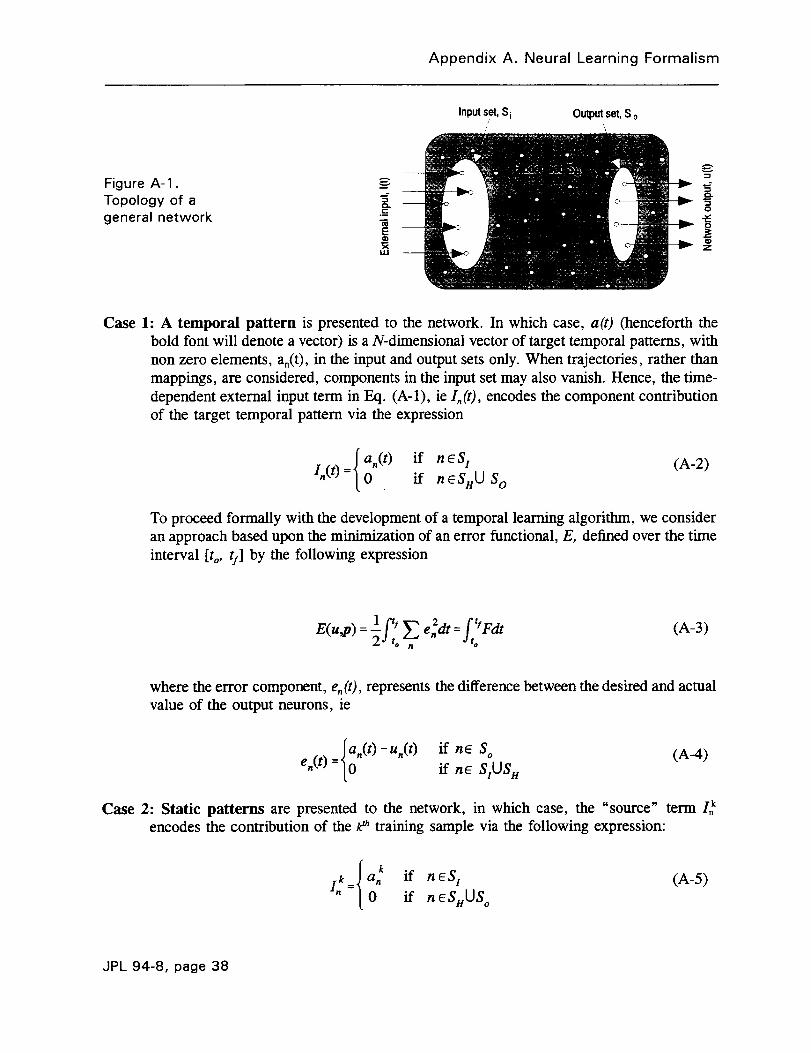
Appendix A. Neural Learning Formalism
Input set, S i Output set, S o/
Figure A- 1.
Topology of a°=general networkE
0.
"50
0
0Z
Case 1: A temporal pattern is presented to the network. In which case, a(t) (henceforth the
bold font will denote a vector) is a N-dimensional vector of target temporal patterns, with
non zero elements, a.(t), in the input and output sets only. When trajectories, rather than
mappings, are considered, components in the input set may also vanish. Hence, the time-
dependent external input term in Eq. (A-l), ie I_(t), encodes the component contribution
of the target temporal pattern via the expression
a.(t) if neS t/.(0= 0 if n eSMU S o(A-2)
To proceed formally with the development of a temporal learning algorithm, we consider
an approach based upon the minimization of an error functional, E, defined over the time
interval [t o, tl] by the following expression
1 y
E( u,p ) = -__o _ e 2.dt = ,_,otiFdt (A-3)
where the error component, e.(t), represents the difference between the desired and actual
value of the output neurons, ie
if n_ S O (A-4)
if ne SzUS n
Case 2: Static patterns are presented to the network, in which case, the "source" term I k
encodes the contribution of the ]#h training sample via the following expression:
ik={ ak. if neS 10 if neSnUS o
(A-5)
JPL 94-8, page 38

Appendix A. Neural Learning Formalism
As in the temporal case, the development of a static supervised learning algorithm
requires minimization of an error function, E, given by the following expression:
2 k n_(ti#- a#) 2 VnqStUS o(A-6)
Where the vector a denotes the steady state solution of the neural activation dynamics,
Eq.(A-1).
In both static and temporal models, the internal dynamical parameters of interest are the
strengths of the synaptic interconnections, T,_, the characteristic decay constants, r., and the
gain parameters, q,n. They can be presented as a vector of M (M = N 2 + 2N) components:
(A-7)P = [Tll, "", TNN' KI' ""'KN_YI' ""' YN]
We will assume that elements of p are statistically independent. Furthermore, we will also
assume that, for a specific choice of parameters and set of initial conditions, a unique solution
of Eq. (A-l) exists. Hence, the state variables u are an implicit function of the parameters p.
In the rest of this document, we will denote the #th element of the vector p by p, (# = 1,-.-,
M) and limit ourselves to the temporal learning case due to its importance to our application.
Traditionally, learning algorithms are constructed by invoking Lyapunov stability
arguments, ie by requiring that the error functional be monotonically decreasing during the
learning time, 7". This translates into
dE__ dE dp_de .=, < 0
(A-8)
One can always choose, with 71 > 0
dp. _ dErl (A-9)
dr. dp,
which implements learning in an inherently local minimization procedure. Attention should be
paid to the fact that Eqs. (A-I) and (A-9) may operate on different time scales, with parameter
adaptation occurring at a slower pace. Integrating the dynamical system, Eq.(A-9), over the
interval [r, T+A_'], one obtains
p.('c +Ar.) = p_,(r.)-rl f _÷_ dE dz, (A-10)" "_ dp p.
JPL 94-8, page 39
Appendix A. Neural Learning Formalism
Equation (A-10) implies that, in order to update a system parameter p_, one must evaluate the
"sensitivity" (ie, the gradient) of E, Eq. (A-3), with respect to p_ in the interval [r, r+Ar].
Furthermore, using Eq. (A-3) and observing that the time integral and derivative with respect
to p, commute, one can write
de _ f,: f,,Or. O.=f': m . --mato :,o Op :,o ,gu Op.
(A-11)
This sensitivity expression has two parts. The first term in the right hand side of Eq.(A-11) is
called the "direct effect", and corresponds to the explicit dependence of the error functional on
the system parameters. The second term in the right hand side of Eq. (A-11) is called the
"indirect effect", and corresponds to the implicit relationship between the error functional and
the system parameters via u. In our learning formalism, the error functional, as defined by
Eq. (A-3), does not depend explicitly on the system parameters; therefore, the "direct effect"
vanishes, ie
aF-0
0p_, (A-121
Since F is known analytically (namely, Eqs. (A-3) and (A-4)), computation of aF/Ou is straight-forward. Indeed
OF- e (A-13)
OU n n
Thus, to enable evaluation of the error gradient using Eq. (A-11), the "indirect effect" matrix
Ou/Op should, in principle, be computed.
In summary, the problem of temporal learning is typically formulated as a minimization,
over an arbitrary but finite interval, of an appropriate error functional. The gradients of the
functional with respect to the various parameters of the neural architecture, eg synaptic weights,
neural gains etc, are essential elements of the minimization process. In the past, major efforts
have been devoted to the efficacy of their computation.
Calculating the gradients of a system's output with respect to different parameters of the
system is, in general, of relevance to several disciplines. Hence, a variety of methods have been
proposed in the literature for computing such gradients. We will briefly mention only thosewhich are relevant to our work.
Williams and Zipser (1989) presented a scheme in which the gradients of an error
functional with respect to network parameters are calculated by direct differentiation of the
neural activation dynamics. This approach is computationally very expensive and scales poorly
to large systems. The inherent advantage of the scheme is the small storage capacity required,
which scales as O(N3), where N denotes the size of the network.
Pearlmutter (1989), on the other hand, described a variational method which yields a set
JPL 94-8, page 40

Appendix A. Neural Learning Formalism
of linear ordinary differential equations for backpropagating the error through the system. These
equations, however, need to be solved backwards in time. It requires temporal storage of
variables from the network activation dynamics, thereby reducing the attractiveness of the
algorithm.
Recently, Toomarian and Barhen (1992) suggested an approach for calculating the
gradients of an error functional with respect to the system's parameters. It builds upon advances
in nonlinear sensitivity theory. In particular, it exploits the concept of adjoint operators to reduce
the computational costs. Two novel systems of equations for error propagation (ie, the adjoint
equations), are at the heart of our computational framework. These equations are solved
simultaneously (ie, forward in time) with the network dynamics. The computational complexity
of the algorithm scales as O(N 3) per time step. The storage requirements are minimal ie, of the
order of O(N2).
JPL 94-8, page 41


REFERENCES
Aleksander, I. (Ed.) (1989). Neural Computing Architectures: The Design of Brain Like
Machines, Cambridge, MA: The MIT Press.
Amari, S. I. (1972). Characteristics of Random Nets of Analog Neuron-Like Elements, IEEE
Trans. Sys., Man, Cyber., SMC-2(5), 643-657.
Amari, S. I. (1979). A Neural Theory of Association and Concept Formation, Bio. Cyber., 26,
175-185.
Amari, S.-I. (1983). Field Theory of Self-organizing Neural Networks, IEEE Trans. Sys., Man,
Cyber., SMC-13(5), 741-748.
Carpenter, G.A. & Grossberg S. (1987a). A Massively Parallel Architecture for a Self-
Organizing Neural Pattern Recognition Machine, Comp. Vis., Gra., and Image Proc.,
37, 54-115.
Carpenter, G.A. & Grossberg, S. (1987b). ART 2: Self-Organization of Stable Category
Recognition Codes for Analog Input Patterns, Applied Optics, 26(23), 4919-4930.
Elgerd, O.I. (1971). Electric Energy Systems Theory: An Introduction, New York: McGraw-Hill.
Graubard, S.R. (1989). The Artificial Intelligence Debate: False Starts, Real Foundation,
Cambridge, MA: The MIT Press.
Grossberg, S. (1987a). The Adaptive Brain, I: Cognition, Learning, Reinforcement and Rhythm,Amsterdam: Elsevier/North-Holland.
Grossberg, S. (1987b). The Adaptive Brain, H: Vision, Speech, Language and Motor-Control,Amsterdam: Elsevier/North-Holland.
JPL 94-8, page 43
olt_ll_',_ PAGE IB!.$d',_3(I'#OT F|L:'-".'Zt_

References
Grossberg, S. (1988). Nonlinear Neural Networks: Principles, Mechanisms, and Architectures,
Neural Networks, 1(1), 17-62.
Hebb, D.O. (1949). Organization of Behavior, New York, NY: John Wiley.
Hofstader, D.R. (1979). G6del, Escher, and Bach, New York, NY: Bantam Books.
Hopfield, J.J. (1982). Neural Networks and Physical Systems with Emergent Collective
Computational Abilities, Proc. Nat. Acad. Sci., 79, 2554-2558.
Hopfield, J.J. (1984). Neurons with Graded Response have Collective Computational PropertiesLike Those of Two-State Neurons, Proc. Nat. Acad. Sci., 81, 3058-3092.
Hopfield, J.J. & Tank, D.W. (1985). Neural Computation and Constraint Satisfaction Problems
and the Traveling Salesman, Biol. Cyber., 52, 141-152.
Kanal, L. & Tsao T. (1986). Artificial Intelligence and Natural Perception, Proc. Intelligent
Autonomous Systems, Amsterdam, 60-70.
Kohonen, T. (1977). Associative Memory: System Theoretic Approach, Berlin: Springer-Verlag.
Kohonen, T. (1982). Self-Organized Formation of Topologically Correct Feature Maps, Biol.
Cyber., 43, 59-70.
Kohonen, T. (1984). Self-Organization and Associative Memory, Berlin: Springer-Veflag.
Kohonen, T. (1987). Adaptive, Associative, and Self-Organizing Functions in Neural
Computing, Applied Optics, 26(23), 4910-4919.
Kohonen, T. (1988). An Introduction to Neural Computing, Neural Networks, 1(1), 3-16.
Ladd, S. (1985). The Computer and the Brain: Beyond the Fifth Generation, New York: Bantam
Books.
Leibniz, J. (1951). Selections, Philip Wiener (Ed.), New York, NY: Scribner.
Linsker, R. (1986a). From Basic Network Principles to Neural Architecture: Emergence of
Spatial-Opponent Cells, Proc. Nat. Acad. Sci., 3, 7508-7512.
Linsker, R. (1986b). From Basic Network Principles to Neural Architecture: Emergence ofOrientation-Selective Cells, Proc. Nat. Acad. Sci., 83, 8390-8394.
Linsker, R. (1986c). From Basic Network Principles to Neural Architecture: Emergence of
Orientation Columns, Proc. Nat. Acad. Sci., 83, 8779-8783.
Lippmann, R.P. (1987). An Introduction to Computing with Neural Nets, IEEE ASSP Magazine,
4(2), 4.
McCulloch, W.S. & Pitts, W.H. (1943). A Logical Calculus of the Ideas Immanent in Nervous
Activity, Bulletin of Mathematical Biophysics, 5,115.
Minsky, M. & Papert, S. (1969). Perceptrons: An Introduction to Computational Geometry,
Cambridge, MA: MIT Press. Prentice-Hall.
Newell, A. & Simon, H. (1976). Computer Science as Empirical Inquiry: Symbols and Search,
Comm. ACM.
Pearlmutter, B.A. (1989). Learning State Space Trajectories in Recurrent Neural Networks,
Neural Computation, 1(3), 263-269.
Rosenblatt, F. (1962). Principles of Neurodynamics, Perceptrons and the Theory of Brain
Mechanisms, Washington, D.C: Spartan Books.
Schleif, F.R. & White, J.H. (1966). Damping for the Northwest-Southwest Tie Line
Oscillations--An Analog Study, IEEE Trans. Power Apparatus and Systems, PAS-85,1239-1246.
JPL 94-8, page 44

References
Schleif, F.R., Hunkins, H.D., Hattan, E.E., & Gish, W.B. (1969). Control of Rotating Exciters
for Power System Damping: Pilot Applications and Experience, IEEE Trans. Power
Apparatus and Systems, PAS-88, 1259-1266.
Stevenson, W.D., (1962). Elements of Power System Analysis, New York: McGraw-Hill.
Toomarian, N. & J. Barhen (1992). Learning a Trajectory Using Adjoint Functions, and
Teacher Forcing, Neural Networks, 5(3), 473-484.
Weiner, N. (1948). Cybernetics, Control and Communications in the Animal and the Machine,
New York, NY: John Wiley and Sons.
Williams, R.J., & Zipser, D. (1989). A Learning Algorithm for Continually Running Fully
Recurrent Neural Networks, Neural Computation, 1(3), 270-280.
Winograd, S. & Cowan, J.D. (1963). Reliable Computation in the Presence of Noise,
Cambridge, MA: The MIT Press.
Winograd, T. (1976). Artificial Intelligence and Language Comprehension, National Institute
of Education, Washington, D.C.
Zak, M. (1988). Terminal Attractors for Addressable Memory in Neural Networks, Physics
Letters A, 133, No. 1,2, 18-22.
Zak, M. (1989a). Terminal Attractors in Neural Networks, Int. J. Neural Networks, 2(3),
Zak, M. (1989b). The Least Constraint Principle for Learning in Neurodynamics, Phys. Lett.
A, 135, 25-28.
Zak, M. (1990). Weakly Connected Neural Networks, Applied Math. Lett., 3(3),
Zak, M. (1991). Creative Dynamics Approach to Neural Intelligence, Biol. Cyber.
JPL 94-8, page 45

TECHNICAL REPORT STANDARD TITLE PAGE,, | i,,
l. Report No. 94-8 1 2. Government..,, Accession No. 3. Reclplent's Catalog No.
4. Title and Subtitle
COMMUNICATION AND CONTROL FOR ELECTRIC POWER SYSTEMSPOWER SYSTEM STABILITY APPLICATIONS OF ARTIFICIAL
5. Report DateApril 1994
6. Performing Organization Code
8. Performing Organization Report No.
NEURAL NETWORKS
7. Author_) N. Toomarian
H. Kirkham
9. Per_rming Organization Name and Address
JET PROPULSION LABORATORY
California Institute of Technology4800 Oak Grove Drive
Pasadena, California 91109
"12. Sponsoring Agency Name and Addres_
NATIONAL AERONAUTICS AND SPACE ADMINISTRATION
Washington, D.C. 20546i, • ii
15. Supplementary Notes
94-810. Work Unlt No.
11. Contract or Grant No.NAST-918
1'3: Type of Report and Period Covered
Final Report
14. Sponsoring Agency Code
16. Abstract
This report investigates the application of artificial neural networks to the
problem of power system stability. The field of artificial intelligence, expertsystems and neural networks is reviewed. Power system operation is discussed with
emphasis on stability considerations. Real-time system control has only recently
been considered as applicable to stability, using conventional control methods.The report considers the use of artificial neural networks to improve the stability
of the power system. The networks are considered as adjuncts and as replacements
for existing controllers. The optimal kind of network to use as an adjunct to a
generator exciter is discussed.
17. Key Wor_ _elected by Author_))Artificial Neural Networks
Power System Control
Power System Stability
Artificial Intelligence
Expert Systems
19. Security Cl_slf. _f'thls repot)
18.'Distrlbution Statement
20. Security Classif. (of thls page) 21. No. of Pages
4S
PAGE li_.AN'R I',K)T FtLI_'Ur-?
22. Price
JPt_ 0184, R _1_