The Relevance of the Seed Capital Investment in aTechnology Based Company

Case Study Analysis of Paydiant

Ricardo Jorge Pereira Bangueses

Thesis to obtain the Master of Science Degree in

Communication Networks Engineering

Examination Committee

Chairman: Prof. Paulo Jorge Pires Ferreira

Supervisor: Prof. Joao Manuel Marcelino Dias Zambujal de Oliveira

Member of the Committee: Prof. Manuel Filipe Mouta Lopes

November 2013

Acknowledgments

I would like to show my greatest appreciation to Professor Joao Zambujal de Oliveira for his availability,

orientation and tremendous support during the whole process of this project. Without his encouragement

and guidance this project would have not materialized. Thanks to him, I have discovered a whole new

scientific field which I ended up loving.

I would like to thank Portugal Telecom Project Manager Pedro Ricarte for introducing me to the

mobile proximity payment industry, providing me some guidelines and showing me a mobile wallet pro-

totype.

I would also like to thank Square Security Engineer Diogo Monica for providing me some market data

and supporting this research.

Furthermore, I am grateful to Professor Manuel Mouta Lopes for his availability and for his help

during the course of investigation.

To Pedro Sa, Barbara Rodrigues, Nuno Nogueira, Luis Salguero, Lucas Gastaldi, Filipe Nogueira and

Nusa Babic for reviewing some parts of this work and providing me with feedback.

To my family, parents and brothers, thank you for always supporting me and believing in me, and for

letting me find my own way.

Resumo

As empresas de base tecnologica sao caraterizadas pela incerteza porque nao ha forma de prever o que

acontecera no futuro. Os investimentos feitos em novas empresas sao tıpicamente irreversıveis, mas podem

ser diferidos por algum tempo. Estes fatores estimulam o uso de tecnicas mais avancadas de analise de

investimento para obter uma avaliacao mais precisa dos investimentos semente.

A perspetiva do investimento faseado leva a investimentos num prototipo, cujo valor e inferior a um

investimento na totalidade. Se as condicoes observadas forem favoraveis, uma opcao de expansao pode

entao ser considerada. Tal decisao teria base na informacao gerada pelo investimento semente, que reduz

a incerteza inerente ao projeto.

Este trabalho fornece um enquadramento para determinar o valor otimo do investimento semente

numa empresa de base tecnologica, reduzindo o capital exposto e planificando o calendario de inves-

timento. Alem disso, este trabalho valida or resultados com recurso a simulacao de Monte Carlo. O

modelo de investimento faseado com uso do filtro de Kalman antecipa a definicao do melhor momento de

investimento. Considerando as condicoes do mercado no qual a Paydiant se integra, o modelo acaba por

antecipar a decisao de investimento.

Palavras-chave: Opcoes Reais, Investimento Semente, Filtro de Kalman, Monte Carlo, Paga-

mentos Moveis por Proximidade, Paydiant.

Abstract

New technology based companies such as Paydiant are characterized by uncertainty since there is no

way of predicting what will undoubtedly happen in the future. Investments made in new companies are

typically irreversible, or at least partially, but can be delayed for a determined amount of time. These

factors stimulate the use of new analysis methods for a more precise valuation of their seed investments.

Taking a phased investment approach may lead to lower initial investment values, hence reducing the

amount of capital at risk. If conditions prove to be favorable, an expansion option could be considered.

Such decision would be based upon new data obtained by the seed investment and therefore under a

reduced level of uncertainty. In addition, a good market performance and a reduced volatility could

anticipate the decision to invest. To sum up, the use of a seed investment with an appropriate size would

require less initial capital and at the same time have an uncertainty reducing effect.

This study provides a framework for determining the optimal value of the seed capital investment

in technology based projects, reducing the capital exposure and planning the investment schedule. Fur-

thermore, it validates the theoretical results from the models through Monte Carlo simulation. The

phased investment model with Kalman filter allows for the anticipation of the best timing of investment.

Considering Paydiant’s market assumptions, the model leads to the anticipation of the investment.

Keywords: Real Options, Seed Investment, Kalman Filter, Monte Carlo, Mobile Proximity

Payments, Paydiant.

Contents

Acknowledgments . . . . . . . . . . . . . . . . . . . . . . . . . . . . . . . . . . . . . . . . . . . . 3

List of Tables . . . . . . . . . . . . . . . . . . . . . . . . . . . . . . . . . . . . . . . . . . . . . . iii

List of Figures . . . . . . . . . . . . . . . . . . . . . . . . . . . . . . . . . . . . . . . . . . . . . v

Nomenclature . . . . . . . . . . . . . . . . . . . . . . . . . . . . . . . . . . . . . . . . . . . . . . viii

1 Introduction to Technology Based Investments 1

1.1 Motivation and Relevance . . . . . . . . . . . . . . . . . . . . . . . . . . . . . . . . . . . . 1

1.2 Problem Definition . . . . . . . . . . . . . . . . . . . . . . . . . . . . . . . . . . . . . . . . 2

1.3 Document Structure . . . . . . . . . . . . . . . . . . . . . . . . . . . . . . . . . . . . . . . 4

2 New Tech-Based Investment’s Literature Review 5

2.1 Valuation Framework Definition . . . . . . . . . . . . . . . . . . . . . . . . . . . . . . . . . 5

2.1.1 Defining a New Technology Based Firm . . . . . . . . . . . . . . . . . . . . . . . . 5

2.1.2 Life Cycle Perspective . . . . . . . . . . . . . . . . . . . . . . . . . . . . . . . . . . 7

2.1.3 Valuation Models Introduction . . . . . . . . . . . . . . . . . . . . . . . . . . . . . 8

2.2 Discounted Cash Flow Models and Decision Trees . . . . . . . . . . . . . . . . . . . . . . . 10

2.3 Real Options Valuation . . . . . . . . . . . . . . . . . . . . . . . . . . . . . . . . . . . . . 11

2.3.1 Black and Scholes Model . . . . . . . . . . . . . . . . . . . . . . . . . . . . . . . . 14

2.3.2 Taxonomy of Real Options . . . . . . . . . . . . . . . . . . . . . . . . . . . . . . . 15

2.3.3 Binomial Pricing Model . . . . . . . . . . . . . . . . . . . . . . . . . . . . . . . . . 16

2.3.4 Monte Carlo Simulation . . . . . . . . . . . . . . . . . . . . . . . . . . . . . . . . . 18

2.4 Phased Investment and Real Options . . . . . . . . . . . . . . . . . . . . . . . . . . . . . . 19

3 Methodological Approach to the Case Study 21

3.1 The Net Present Value and Option Pricing . . . . . . . . . . . . . . . . . . . . . . . . . . 21

3.2 Introduction to the Investment Models . . . . . . . . . . . . . . . . . . . . . . . . . . . . . 22

3.3 Single Investment Model . . . . . . . . . . . . . . . . . . . . . . . . . . . . . . . . . . . . . 24

3.4 Two-Phased Investment Model . . . . . . . . . . . . . . . . . . . . . . . . . . . . . . . . . 28

3.5 Two-Phased Investment Model With Kalman Filter . . . . . . . . . . . . . . . . . . . . . 31

4 Case Study Analysis and Description: Paydiant 35

4.1 Payment Industry Evolution and Paydiant . . . . . . . . . . . . . . . . . . . . . . . . . . . 35

i

4.2 Investment Assumptions . . . . . . . . . . . . . . . . . . . . . . . . . . . . . . . . . . . . . 41

4.2.1 Expected Market Evolution . . . . . . . . . . . . . . . . . . . . . . . . . . . . . . . 41

4.2.2 Costs and Revenue . . . . . . . . . . . . . . . . . . . . . . . . . . . . . . . . . . . . 43

4.2.3 Volatility . . . . . . . . . . . . . . . . . . . . . . . . . . . . . . . . . . . . . . . . . 45

4.3 Results of the Investment Models . . . . . . . . . . . . . . . . . . . . . . . . . . . . . . . . 47

5 Conclusions 53

Bibliography 58

ii

List of Tables

2.1 Analogy between Financial Options and Real Options. . . . . . . . . . . . . . . . . . . . . 12

2.2 Effects of increasing variable values in options. . . . . . . . . . . . . . . . . . . . . . . . . 14

4.1 2008 Survey of consumer payment choice. . . . . . . . . . . . . . . . . . . . . . . . . . . . 36

4.2 United States consumer payment systems. . . . . . . . . . . . . . . . . . . . . . . . . . . . 37

4.3 Mobile transaction volume worldwide. . . . . . . . . . . . . . . . . . . . . . . . . . . . . . 41

4.4 Proximity mobile payment forecast growth rates. . . . . . . . . . . . . . . . . . . . . . . . 41

4.5 U.S.A. debit, credit and prepaid cards market data. . . . . . . . . . . . . . . . . . . . . . 42

4.6 Average value of transactions by type of magnetic stripe card. . . . . . . . . . . . . . . . . 42

4.7 Expected evolution of demand. . . . . . . . . . . . . . . . . . . . . . . . . . . . . . . . . . 42

4.8 Average value of magnetic stripe card percentage fees by instrument. . . . . . . . . . . . . 43

4.9 Estimated costs for a data center and for a cloud computing service. . . . . . . . . . . . . 45

4.10 Estimated U.S.A. debit card transaction volume and growth rates. . . . . . . . . . . . . . 46

4.11 T-test results for the smallest investment size. . . . . . . . . . . . . . . . . . . . . . . . . . 47

4.12 Summary of the models’ parameters. . . . . . . . . . . . . . . . . . . . . . . . . . . . . . . 48

4.13 Outcome for the single investment model. . . . . . . . . . . . . . . . . . . . . . . . . . . . 48

4.14 Outcome for the phased investment model. . . . . . . . . . . . . . . . . . . . . . . . . . . 49

4.15 Impact of the Kalman filter on the seed investment models’ variance. . . . . . . . . . . . . 50

4.16 Impact of the Kalman filter on the seed investment models’ optimal hedged capacity. . . . 51

4.17 Phased investment models’ demand values that trigger the expansion decision. . . . . . . 51

iii

iv

List of Figures

2.1 Geoffrey Moore’s technology adoption curve . . . . . . . . . . . . . . . . . . . . . . . . . . 8

2.2 Decision tree example: FedEx’s expansion option expressed as a simple decision tree . . . 11

2.3 Binomial option pricing example . . . . . . . . . . . . . . . . . . . . . . . . . . . . . . . . 16

4.1 U.S.A. mobile phone subscribers by device. . . . . . . . . . . . . . . . . . . . . . . . . . . 38

4.2 U.S.A. proximity mobile payment transaction values. . . . . . . . . . . . . . . . . . . . . . 40

4.3 Effect of the Kalman filter on the variance through time. . . . . . . . . . . . . . . . . . . . 50

4.4 Value of the project depending on the timing of the investment. . . . . . . . . . . . . . . . 52

v

vi

Nomenclature

Greek symbols

α, αs Market trend rate coefficient, statistical significance.

β Positive root of the quadratic partial differential equation.

δ Option delta, convenience yield.

εt White noise.

µ Mean value of the sample.

Ω Average value per transaction.

Π (•, •) Cash flow function.

ρ Expected rate of return.

σ Standard deviation.

θ Stochastic variable, hedged capacity.

θ0 Initial hedged capacity.

Roman symbols

A Value of the underlying asset.

a Investment function coefficient, setup cost.

b Cost per each transaction processed.

C Cash outflow; value of the call option.

c, k Fixed cost function coefficients.

D Transaction demand.

E [•] Mathematical Expectancy.

F (•, •) Value of the option.

G (•, •) Processing capacity cost function.

vii

Ht Observed value in t.

I, I (•) Investment function, setup cost for a given size.

K Processing Capacity.

K0 Smallest seed investment transaction processing capacity.

Km Minimum Processing Capacity.

m Margin per each transaction processed.

p Risk neutral probability, revenue from each transaction processed.

R Cash inflow.

r Minimum acceptable rate of return, risk-free rate.

St Conditional variance.

sx Standard deviation of the sample.

T, t Maturity, time.

V, Vt, V (•, •) Value of the investment project at time t.

W,X Wiener process.

X Option strike price.

Zt Representative function of the cumulative observations.

Subscripts

s, p, k Investment model: single, phased and with Kalman filter.

t In a given time t.

u, d Up and down movements.

Superscripts

* Optimal value.

viii

Chapter 1

Introduction to Technology Based

Investments

1.1 Motivation and Relevance

During the 90’s industrial and natural resource giants were the largest companies in terms of market

capitalization (Damodaran, 2001). However, at the beginning of 2000 there was a shift towards technology

based companies where six of the ten largest firms were technology based1. This shift was preceded by

the information technology bubble, where investors poured money into technology based firms in the

hope that they would become profitable. During this period, the NASDAQ2 composite index rose from

776.80 to 4696.69, a 605% increase heavily influenced by prices in high-technology stocks (Galbraith &

Hale, 2003).

The development of technology based projects goes through a sieve of technical tests, capable of

measuring the value of the idea behind it. One of the tests the project must pass is the market, where the

acceptance of the project output is evaluated among the consumers, typically with the use of prototypes.

In these tests the value of the technological innovation and the amount of investment needed for the

success of the project is settled.

Seed capital investments usually happen after the prototype phase, where the amount of capital

to be invested depends on the number of failures in the prototype. A fast evolution of the prototype

usually means a greater support from a Venture Capital company and a greater likelihood of passage into

production phase.

Dolan and Giffen (1988) argue that the determination of the seed-capital investment needed for

a new project is not only important for big companies but also for small entrepreneurs. New ventures,

particularly those in high-risk sectors, lack of appropriate management skills and have difficulties accessing

seed-capital financing. Ironically, successful start-ups in these areas make significant contributions to

economic diversity and employment3.

1By January 2000 Cisco, Microsoft, Oracle, Intel, IBM and Lucent where among the ten largest firms in the U.S.A.2National Association of Securities Dealers Automated Quotations.3NVCA. ’Venture Impact: The Economic Importance of Venture Capital-Backed Companies to the US Economy’, 2011.

1

In the United States, the success of venture capital-supported companies like Microsoft and Apple

fueled further success. Chip maker Intel, for instance, has its own venture capital arm. Intel Capital

has gone on to seed-fund companies like Research In Motion, the company behind the development of

the BlackBerry. The National Venture Capital Association in the U.S.A. states venture capital-backed

companies employ more than twelve million people (around 11% of private sector employment) and

generate nearly three trillion dollars in revenue (around 21% of U.S.A. Gross Domestic Product)4.

Apple Inc. recent innovative projects, the iPhone and the iPad, are another case of success. In July

2011 Apple managed to have an operating cash balance greater than that of the U.S.A. government5. Its

Third Quarter report on the same month announced a record quarterly net profit of $7.31 billion. During

this quarter the company sold 20.34 million iPhones, representing a 142% growth over a year ago. The

same report mentioned a 183% growth on its iPad sales, its most innovative gadget6.

However, the lack of proper analysis and valuation techniques may contribute to a lackluster return

on investment on start-ups. Examples of these were widely present in the information technology boom

and bust in the late 90’s; Boo.com spent $188 million in just six months in an attempt to create a

global fashion store, filing bankruptcy later on7. Another example was that of The Learning Company,

purchased by Mattel in 1999 for $3.5 billion and sold a year later for only $27.3 million8.

Innovation continues to transform the mobile phone industry at an astounding pace. The smartphones

processing speed and connectivity are being constantly improved, becoming efficient multi-utility pocket

PCs. This evolution prompted the incorporation of other technologies into the devices, such as Global

Positioning System and Near Field Communication, and the development of a huge number of applications

with varying goals.

The electronic payment industry has been on the rise over the years. In 2005 it represented over 49%

of all the volume transacted in the United States, while in 2010 it accounted for 61%9. On the other

hand, the use of cash has had a slight decline over the same period, representing only 19% of the volume

transacted (from 21% in 2005), while the use of checks declined from 28% to 18%. As a result, the

payment processing industry has become an alluring target for companies such as Paydiant, who intend

to tap into this industry which accounts for thousands of billions of dollars.

1.2 Problem Definition

The market of products or services provided by an innovative idea is typically unknown. An initial

investment on an Information Technology or Research and Development project serves as a way of

collecting information about the market targeted (Cukierman, 1980; Demers, 1991; Luehrman, 1998).

This information allows for a better management of investment or deferral decisions, which help avoiding

over-sizing or under-sizing the production output.

4See footnote 3.5BBCNews. ’Apple holding more cash than USA’, July, 2011.6Apple Inc Third Quarter Results Report, July, 2011.7New York Times. ’Fashionmall.com Swoops In for the Boo.com Fire Sale’, June, 2000.8Los Angeles Times. ’Mattel Settles Shareholders Lawsuit for $122 Million’, December, 2002.9The Nilson Report, ’U.S. Consumer Payment Systems in PCE’, 2011.

2

By exploring the relationship between seed-capital investment and its uncertainty reducing effect,

we can try to minimize the cost of the initial investment in a technology based project. Investing in a

traditional way, i.e. using traditional methods such as discounted cash flows, would force us to commit a

bigger amount of capital. In addition, these methods also fail to capture the intrinsic value of flexibility

(Koller et al., 2005).

Since technology based projects are typically characterized by uncertainty, managers may take advan-

tage of the responding market and adapt accordingly, turning it into a highly profitable venture (Neelly

& Neufville, 2001). Moreover, a phased investment strategy combined with managerial flexibility reduces

the risk of the endeavor and as a result, there is less capital exposure if the profitability turns out to be

lackluster.

When dealing with a new product or service we must take into account uncertainties in production

and commercialization. These could be defined as the lack of market information, production techniques

or raw materials used. Any financial attempt to gather market information or production improvements

represents a risk to the economic viability of the project. This risk is defined by the technical uncertainty

on production and economic uncertainty on commercialization (Lopes, 2007).

Technical uncertainty can be reduced by what is called learning by doing: investing in order to find

the right materials and improve techniques. Numerous authors argue that the technical uncertainty

decreases as time goes by, without the project manager intervention (Bernanke, 1983; Demers, 1991;

Dixit & Pindyck, 1994; Kulatilaka & Perotti, 1998; Grenadier, 1999). However, economic uncertainty

can be reduced by either observing the market behavior from the outside - learning by waiting - or by

investing. An initial small investment may reduce or eliminate this uncertainty by providing information

about the market behavior (Luehrman, 1998). Using this information, the manager may estimate the

time and size of the expansion, expanding the production output gradually until it accommodates the real

demand (Demers, 1991). However, this information may also point to the anticipation of the investment

decision due to the competition (Grenadier, 1999).

Valuing Information Technology (IT) projects is a particularly challenging task because there are

many factors that affect their payoffs and costs. They usually involve the acquisition or development

of multiple assets of different nature, such as infrastructure and application software, that might have

little or no value unless other assets are present. Even when the benefits of a particular asset can be

isolated from other decisions taken with respect to the IT infrastructure, the benefits and costs of an IT

project have a high degree of uncertainty because their realization is affected by multiple organizational

elements. There are also multiple alternatives for the development of projects that imply different phases

and cost schemes. Choosing among these alternatives has implications on the options available for the

project manager once the project has started (Schwartz & Zozaya-Gorostiza, 2000).

The purpose of this work is to provide a framework which determines the critical values of the seed

capital investment in technology based projects, reducing the risk and planning the investment schedule.

We propose to validate a two phased investment model based on a Real Options approach by applying it

to our case study. This model works on the premise that the seed investment has an uncertainty reducing

effect. By exploring this uncertainty reducing effect it will provide the critical timing of the investment.

3

Afterwards it will attempt to determine an adequate amount of seed capital needed to maximize the

investment.

1.3 Document Structure

The next chapter, New Tech-Based Investment’s Literature Review, describes the critical points of knowl-

edge related to the valuation techniques in technology based start-ups. It defines the new technology

based company concept, provides the life-cycle perspective and introduces some valuation models. Due to

the limitations of the traditional models we will consider a model based on Real Options theory. Hence

we also describe in detail the basic concepts and relevant models that are related to a Real Options

approach. Chapter 3 then describes the methodological approach to the case study, with an introduction

to the investment models and the three investment models we will consider: the single investment model,

the phased investment model and the phased investment model with the Kalman filter. Next, in chapter

4, we describe our case study, Paydiant, and its market. We also present the assumptions required in the

valuation and then the outcomes from the models. Finally, chapter 5 states our conclusions.

4

Chapter 2

New Tech-Based Investment’s

Literature Review

2.1 Valuation Framework Definition

The following paragraphs define the terms and introduce us to some models relevant to this research.

Technological innovation projects are typically done by technology based firms. The seed investments

are, by definition, made at a specific stage of a firm’s life-cycle. Subsection 1 starts by defining these

technology based firms. Subsection 2 describes the typical firms’ life-cycles, and subsection 3 concludes

with an introduction to some valuation models.

2.1.1 Defining a New Technology Based Firm

The term New Technology Based Firm (NTBF) seems to have been coined by the Arthur D. Little Group,

who defined it as “an independently owned business established for not more than 25 years and based on

the exploitation of an invention or technological innovation which implies substantial technological risks”

(Little, 1977). Over the decades, this definition has been vastly extended and therefore we should start

by defining other similar forms of organizations: start-ups, spin-offs and Small and Medium Enterprises

(SME).

A start-up is the name given to a company which is in its initiation phase. A wide definition of

start-ups encompasses all firms in an early life-cycle phase, and may also refer to recently incorporated

enterprises characterized through a high level of dynamics and future orientation (Hommel & Knecht,

2002).

A spin-off is a particular type of start-up that originates out of an existing organization, such as a

university, government agency or a company. The spin-off firm is typically associated with a technology

transfer, manpower and other resources (Gassman et al., 2003).

A SME is the result of a surviving start-up at some point in time, depending on the business field

and technology-intensity. The number of employees and the company’s turnover seem to be the most

5

appropriate quantitative criteria to define SMEs (Savioz, 2002). Although quantitative definitions are

very clear, companies end up being considered black boxes. Alternatively, qualitative criteria such as the

identity of ownership and personal responsibility for the enterprise’s activities may help to strengthen the

understanding of SMEs (Luggen, 2004). A SME is the most general term under which start-ups, spin-offs

and NTBFs can be included.

The term NTBF can be defined as the junction of two independent sub-terms: new and technology

based. Luggen (2004) found that in literature there is a quantitative and qualitative approach to de-

scribing the term “new”. Various authors suggest the use of the age limit of the firm as a quantitative

criteria, albeit with different time frames: Artmann et al. (2001) place the limit from 1 to 6 years, Fontes

& Coombs (1997) from 1 to 15 years and Little (1977) from 0 to 25 years. However, the qualitative

approach is based on the firm’s activities where the “new” refers to the typical structure and behavior

of firms in the early phases of their life-cycles (Artmann et al., 2001; Quinn & Cameron, 1983). The

discussion about quantitative and qualitative criteria for the definition of firms to be considered “new”

shows that a generally accepted definition does not exist, hence the limits have to be set according to the

research focus (Luggen, 2004).

Literature often uses terms like “technology based” or “technology intensive”, but Luggen (2004) ar-

gues that there isn’t a generally accepted definition because most contributions that are about technology

based firms do not define them. Chabot (1995) examines the use of “high-technology” based on numerous

authors and thus differentiates between input-based and output-based definitions.

According to Chabot (1995), two major factors drive input-based analysis: R&D expenditure and

occupational profile statistics. These approaches have the advantage of having a straightforward analysis,

provided proper data is available. By counting gross R&D expenditures or calculating the number of

technical staff, it is easy to arrive at an ordered spectrum of technology based and non-technology

based companies. For instance, the OECD classification is one example of input-based analysis on R&D

expenditures. In it, the limit between low-technology and high-technology is 3.5% and the limit between

high-technology and leading-technology is 8.5% (OECD, 1997).

Output-based definitions classify high-technology based on the productive value added output of com-

panies. The actual products of intense R&D, rather than the currency input, drive the essential meaning

of high-technology. Chabot points at two important disadvantages to the output-based approaches,

which explains in part the relative abundance of input-based methods. First, output-based definitions

rely on neither highly accessible nor easily processed data. The second disadvantage is the high decree

of subjectivity.

As for “new”, there is no generally accepted definition of technology based. Quantitative approaches

such as R&D expenditure as percentage of turnover do not make sense in a NTBF, because there is nor-

mally no steady turnover. NTBFs run an innovation process which transfers scientific research findings

into technological products, which are then commercialized. According to the input-output based defini-

tion of technology based, an NTBF has major research projects which lead to innovative new products

(Luggen, 2004). This is the definition that we will consider for the purpose of this work.

Damodaran (2001) provides another definition of technology based firm. He makes a distinction be-

6

tween two groups of companies: one group delivers software and hardware while the other uses technology

to deliver its products or services. Retail companies like Walmart or Carrefour use websites to sell their

products. In fact, most companies now use the internet to reach out to more customers. However, the

fact that they use technology doesn’t mean they are considered technology based firms. In order to make

a distinction, we can define a technology based company as one that makes money by selling products

based on applied scientific knowledge, that is, its source of income comes from the technology developed.

2.1.2 Life Cycle Perspective

Day (1981), Bass (2004), Kotler & Keller (2001) define the product life-cycle as a bell curve where there

is a high demand for the product in the beginning, followed by a slowdown of demand when it reaches

maturity until it starts declining. In the early stage of a particular innovation growth is relatively slow

as the new product is trying to establish itself (Agarwal & Audretsch, 2001). At some point, when the

project is established in the market there is an increase in demand and the product growth increases

rapidly. Narayanan (2001) argues that incremental innovations or changes to the product may bring

further income and allow growth to continue, but towards the end of the technology life-cycle growth

slows and may begin to decline.

To illustrate, a decade ago Nokia was the dominant supplier of cell phones. It beat other suppliers by

combining diversified offerings of handsets with efficient manufacturing and strong customer relationship

management. Nonetheless, its success was within one technology life-cycle because it failed to plan for and

make the transition to the next major technological product, the smartphone. There was a shift of critical

attributes like operating system and software, whereas Nokia focused on basic design and manufacturing.

Competitors like Apple, Samsung, Microsoft and Google took a huge part of the market share, provoking

the collapse of Nokia’s supply chain and forcing it to partner with Microsoft in an attempt to catch

up1. Approximately two years and a half later on Microsoft announced it will purchase substantially

all of Nokia’s Devices & Services business, license Nokia’s patents, and license and use Nokia’s mapping

services2. The Finnish phone maker that once dominated the global market was swallowed by the U.S.

software giant because it failed to adapt against its rivals Apple Inc and Samsung Electronics.

In Crossing the Chasm, a book closely related to the technology adoption life cycle, Moore (1991)

recognizes five main segments: innovators, early adopters, early majority, late majority and laggards.

According to Moore (1991), each of these groups should be targeted at a time, using each group as

a base for marketing to the next group. The most difficult step is making the transition between the

early adopters and the early majority. If a company is able to create a bandwagon effect with enough

momentum then the product becomes a de facto standard. However, Moore’s (1991) theories are only

applicable for disruptive innovations. A disruptive innovation is a type of innovation that helps create a

new market and value network, and eventually goes on to disrupt an existing market and value network,

displacing other (older) technology.

1Microsoft, ’Nokia and Microsoft Announce Plans for a Broad Strategic Partnership to Build a New Global MobileEcosystem’, February, 2011.

2Microsoft, ’Microsoft to acquire Nokia’s devices & services business, license Nokia’s patents and mapping services’,September, 2013.

7

Figure 2.1: Geoffrey Moore’s Technology Adoption Curve, (Moore, 1991).

Traditionally, if a company has reached a maturity state we can use its current financial statements, its

past history and information about its competitors to value the company. Having substantial information

from all three sources would be optimal for the valuation (Damodaran, 2001). Yet a NTBF has a very

limited history, its financial statements do not reveal much about the future growth and any information

about its competitors, if there are any, will most likely be impossible to get. These factors contribute to

a higher uncertainty, encouraging the emergence of new techniques of valuation based upon the limited

information available.

2.1.3 Valuation Models Introduction

Technology based projects are characterized by uncertainty and this uncertainty is one of the reasons

which stimulates companies to increasingly sharpen their analysis methods (Saito et al., 2010). Some of

these techniques are Discounted Cash Flow analysis (DCF), Real Options Valuation (ROV) and Decision

Tree Analysis (DTA). When using a DCF model, only the most likely or representative outcomes are

modeled, and the flexibility available to management is ignored. These methods normally do not properly

account for changes in risk over a project’s life-cycle and fail to appropriately adapt the risk adjustment3.

By contrast, Decision Tree Analysis values flexibility by incorporating possible events or states and

consequent management decisions. For instance, a company would build or expand its factory given that

the demand for its product exceeded a certain level during the pilot phase, or outsource part of its pro-

duction otherwise. In a DCF model every scenario must be modeled separately, there is no “branching”.

Yet in a DTA each management decision in response to an event or situation generates a path which the

company could follow, and the probabilities of each event are specified by management. Once the deci-

sion tree is constructed “all” possible events and their resultant paths are visible to management. Given

this “knowledge”, management chooses the actions corresponding to the highest value path probability

weighted. Hence the path chosen is taken as representative of the project value (Kirkwood, 2002).

Real Options Valuation, often termed Real Options Analysis, applies option valuation techniques to

capital budgeting decisions. This theory states that a real option is the right, but not the obligation, to

undertake a business decision. Some of these decisions are to make, abandon, expand or contract a capital

investment. By doing this it explicitly addresses the inherent managerial flexibility in a project. This

3IBM, ’Calculating value during uncertainty: Getting real with real options’, Accessed 14th, April 2013.

8

methodology is typically used when the value of a project is dependent on conditions or occurrences not

yet established. The ROV approach allows the valuation of flexibility at certain key decision points by

providing the ability to exercise the available options (Brealey & Myers, 2003). By building a clear picture

of what might happen in the future, as well as the contingent strategic decisions, the management and

implementation on the project becomes simpler, clearer and optimal. Koller et al. (2005) state that this

model is an attractive complement to the standard deterministic valuation approaches such as the DCF

model, Monte Carlo Simulation and Decision Tree Analysis. Since it explicitly addresses the inherent

managerial flexibility present in projects, it is most valuable to apply when there is high uncertainty with

regard to the underlying asset value and the benefits that will result from investing in such asset.

The managerial flexibility provided by DTA and ROV approaches is important because it lets man-

agers defer or change investment decisions as a business or project develops (Koller et al., 2005). It can

alter the value of the business or project substantially, while a standard DCF analysis fails to account for

the impact of the flexibility on present value. Knowing the best time to invest helps a company maximize

its profits and minimize its losses, which contribute to the success of the project.

The Net Present Value (NPV) technique is often used to decide whether to invest or not by calculating

the present value of the expected stream of profits and expenditures required. By determining the

difference between the two you get a value which, if greater than zero, indicates a positive investment.

This method’s efficiency has been strongly criticized by Dixit & Pindyck (1994), who argue that the

use of this method may induce wrong investment decisions. They mention two important characteristics

ignored in the investment decision: Irreversibility, the fact that an investment might not be retrieved

in full in case of regret; and the possibility of deferring the investment decision. These features, along

with the uncertainty about the future, allows for an analogy between an investment opportunity and a

financial option.

Dixit & Pindyck (1994) further explain that an entity should have the right, not the obligation, to

invest in a project. By having to choose one of the two options, invest or defer, the choice represents a lost

opportunity cost by not exercising the other, and ignoring this cost may lead to significant error. Under

the Real Options Analysis, the option to invest or defer would be taken when the value of one is greater

than the other. The option of deferring an investment does not exclude the option of investing later,

when the conditions change and the project becomes more suitable. The same does not happen when the

option of investment is taken, since most investments cannot be fully recovered (Dixit & Pindyck, 1994;

Luehrman, 1998; Hull, 1999).

Real Options Valuation (ROV) will be used in this paper due to the limitations of the traditional

methods. ROV offers a more effective analysis of a technology-based project due to its dynamic approach

to project valuation. ROV is not a substitute of any traditional methods, instead it uses DCF and DTA

methodologies as constituents. The value of the options depend on the future management decision

opportunities created by uncertainty. Unlike DTA, the probabilities of each option are dictated by the

volatility of the future cash flows of the project. Also, in contrast with traditional cash flow valuation

techniques, uncertainty increases the value of real options. The higher the uncertainty, higher the option

value and higher the upside potential.

9

2.2 Discounted Cash Flow Models and Decision Trees

Discounted cash flow models (DCF) are considered the main approaches to value projects in traditional

financial methodology. The reason being a DCF analysis is intuitive and straightforward to apply and

consequently most companies use DCF models. Discounted Cash Flow valuation relies on the fact that

one monetary unit today is worth more than one tomorrow. Cash flows associated with a project can

be discounted at time value money to express their values at present (Jeffery, 2004). The rate of return,

which is the interest rate at which the cash flows are discounted, reflects the amount of risk associated

with the cash flow.

The Net Present Value is one of the traditional methods used in capital budgeting to analyze the

profitability of an investment. It’s basically the difference between the sums of the cash inflows and the

cash outflows discounted to their present value using a minimum acceptable rate of return. This model

may be used to choose between projects happening at about the same time, where the higher valuation

nets a greater value from the investment

Other Discounted Cash Flow models for different purposes include: the Internal Rate of Return (IRR)

is useful to compare between one investment or another by calculating the expected rate of growth of

a project; the Payback Period model serves as a way of calculating how long a project will pay itself;

the Profitability Index attempts to identify the relationship between the costs and benefits of a proposed

project through the use of a ratio of amount of money invested to profit of the project.

Damodaran (2001) argues that a DCF valuation fails to consider the decisions embedded in many

projects. A DCF model applied to a young start-up firm in a large market may not reflect the possibility,

as small as it might be, that it becomes the next Google or Apple. Another example would be of a

R&D company with patents; a DCF valuation may under-value it because the expected cash flows do

not consider the possibility that the patent could become extremely valuable in the future. In both cases

a DCF valuation would under-value these companies because it ignores the option to invest more in the

future and take advantage of unexpected success in their businesses (Brealey & Myers, 2003; Damodaran,

2001).

A decision tree is a support tool which can facilitate investment decision making when uncertainty

prevails, specially when the problem involves a sequence of decisions. They provide an effective structure

in which alternative decisions and the implications of taking those decisions can be laid down and evalu-

ated. They may also help forming an accurate estimation of the risks and rewards that can result from

a particular choice (Magee, 1964).

When delineating a tree, each decision point has its alternatives available for experimentation and

action, with investment outlays associated with them. Any decision will have their possible outcomes

associated to, with their estimated probability and their monetary values. This method clearly lays out

the problem so that all known options can be challenged (Chandra, 2008). Hence, DTA allows the investor

to analyze the possible consequences of a decision, while providing a framework to quantify the values of

outcomes and their probabilities. Kirkwood (2002) expresses this type of analysis requires common sense

and the use of real probabilities, or else it might be misleading.

10

Figure 2.2 represents a scenario where FedEx acquires the right to buy and have a plane delivered

from 2008 to 2011. During that period, FedEx may observe the demand for airfreight and decide to

expand by buying the reserved plane, or just allow it to expire by not taking the delivery until 2011.

Figure 2.2: FedEx’s expansion option expressed as a simple decision tree, adapted from Brealey & Myers(2003).

Decision Tree Analysis is able to deal with multiple uncertainties by allowing the mapping of complex

problems. However, it does not provide the true value of the project and may become overwhelming if

the number of branches is too high. Nevertheless, decision trees are commonly used to describe the real

options embedded in capital investment projects (Brealey & Myers, 2003).

2.3 Real Options Valuation

Companies make money by investing capital to exploit profit opportunities. Investments in R&D can

lead to patents and new technologies that bring the option of further investment. Companies in a new,

volatile market may find themselves in a situation where it is best to wait and see how the market

evolves, and expand when the opportunity arrives. Also, shutting down money-losing operations may

also be considered as an investment opportunity, where the initial cost is the price of shutting down and

the payoff is the reduction of future losses.

Brealey & Myers (2003) argue that we cannot simply apply a Discounted Cash Flow method for

valuing these investments because their risk changes over time and it is impossible to discount them at

the opportunity cost of capital. Dixit & Pindyck (1995) also criticize the net present value approach;

while it is relatively easy to apply, it is often wrong because it is built on faulty assumptions: either

that the project is reversible or irreversible. Some investments may fall into this category, but most are

irreversible and capable of being delayed. This capability can profoundly affect the decision to invest,

which undermines the validity of the net present value rule.

The Real Options Theory adapts the techniques developed for financial options to real life decisions.

The term was first conceived by Myers to emphasize that investment opportunities are options on real

assets (Triantis & Borison, 2001). This approach views a project as a process where managers can

continually change its course. This perspective contrasts with traditional models which typically set

decisions at the beginning that remain constant during the project’s life (Neelly & Neufville, 2001).

11

The Real Options Theory recognizes that risks can be managed and allows the manager to take

advantage of good outcomes when they become apparent. As a result, it naturally leads to higher values

when compared to traditional DCF methods. The reason being that a Real Options model incorporates

the ability to minimize losses and maximize gains, therefore leading to a higher perception of value of

risky projects (Neelly & Neufville, 2001).

Dixit & Pindyck (1994), Luehrman (1998), Hull (1999), Lint & Pennings (2001) make an analogy

between corporate investments and financial options. They consider a corporate investment opportunity

like a call option because the corporation has the right, but not the obligation, to exploit an opportunity.

If we could find a call option sufficiently similar to the investment opportunity it would tell us something

about the value of the opportunity. Unfortunately, it is unlikely that such option exists since most

business opportunities are unique, so the most reliable thing we can do is construct our own option. To

do so, Luehrman (1998) suggests obtaining a model of the project that combines its characteristics onto

the template of a call option. To do so, we need to establish a correspondence between the project’s

idiosyncrasies and the five variables that determine the value of a simple call option on a share of stock.

By mapping the characteristics of the business opportunity onto the framework of a call option, we

can obtain a model of the project that combines its characteristics with the structure of a call option

(Luehrman, 1998). To illustrate, a two-phased investment can be seen as a call option whose price is the

seed investment and whose exercise price is the cost of expansion. The expiration date will be the time

until this investment opportunity disappears. Moreover, the variance of the product’s trend will define

the volatility of the underlying asset. Table 2.1 provides several analogies between real and financial

options which allow for the mapping of a business opportunity:

Financial Option Real OptionTime to expiration Length of time the decision may be deferred

Exercise price Expenditure required to acquire the project assetsVariance of stock returns Riskiness of the project assets

Stock Price Present value of a project’s operating assets to be acquiredRisk-free rate of return Time value of money

Dividends Value lost by waiting to invest

Table 2.1: Analogy between Financial Options and Real Options, adapted from Luehrman (1998); Lint& Pennings (2001).

Fisher Black and Myron Scholes published in 1973 their path-breaking paper providing a model for

valuing dividend-protected European options (Black & Scholes, 1973). They used a replicating portfolio,

composed of the underlying asset and the risk-free asset that had the same cash flows as the option being

valued, to come up with their final formulation. The replication portfolio consists of setting up an option

equivalent by combining common stock investment and borrowing. The net cost of buying the option

equivalent must equal the value of the option. Furthermore, the pay-off from levered investment in the

stock is identical to the pay-off from the call option, meaning both investments must have the same value.

To value the option we borrow money and buy stock in such a way that we replicate the pay-off from a

call option. The number of shares needed to replicate one call is called the hedge ratio or option delta(δ):

12

δ =Cu − CdSu − Sd

(2.1)

where C represents the value of the call option, S represents the value of the stock, and the subscripts

represent either their values when they go up u or down d. Once we know the option delta value, we can

calculate the value of the option C :

C = X ∗ δ − X − δ ∗X1 + r

(2.2)

where X is the option strike price, X ∗ δ is the value of underlying asset, r is the interest rate and

X−δ∗X1+r represents the bank loan.

With these expressions we are able to value a simple option, given that we know their possible pay-off.

We can also replicate an investment in the option by a levered investment in the underlying asset. We can

create a home-made option by using a replicating strategy, buying or selling delta shares and borrowing

or lending the balance (Brealey & Myers, 2003).

Option contracts may have different terms or agreements. There are two main types of financial

options: European options and American options. American options may be exercised at any given time

prior to their expiration date, while European options can only be exercised at expiration date. Hence

any model used to appraise options must take into account its type of option (Oliveira, 2012). Moreover,

a real option has its own environment and variables so it will only expire when the investment opportunity

disappears.

In option valuation there are two types of options: call options and put options. A call option provides

its holder the right to buy the underlying asset at a fixed price, called strike or exercise price, before its

exercise date. If the value of the asset is always lesser than the strike price paid for the option, it will

end up expiring worthless. On the other hand, if the value of the asset is greater than the strike price,

the option holder can exercise its right, netting the difference between the asset value and the strike

price (Brealey & Myers, 2003). In an opposite way, the put option gives its holder the right to sell an

asset at the strike price. In this case if the value of the asset is lesser than the strike price, it will net

the difference between the strike price and the market value of the asset. Yet having a greater value of

the asset than the put strike price will render the option worthless once it reaches its expiration date

(Damodaran, 2001).

The option’s value is determined by a number of variables relating to its underlying asset and financial

markets. Options are assets that derive value from their underlying asset, hence any change in the

underlying asset’s value will affect the option’s value. An increase in the value of the underlying asset

will increase the value of the call options and decrease the value of put options. Moreover, options are

also different from other securities in the sense that buyers of options never lose more than the option’s

price. For this reason the volatility may translate into an increase in option value (Damodaran, 2001).

Table 2.2 shows the effect of an increase in the value of the variables in both call and put option value.

13

Increase in Call Option Put OptionAsset value Increases DecreasesExercise price Decreases IncreasesInterest rate Increases IncreasesTime to expire Increases IncreasesVolatility Increases DecreasesDividends Decreases Decreases

Table 2.2: Effects of increasing variable values in options, adapted from Brealey & Myers (2003).

The value of the underlying asset is expected to decrease if dividends are paid on that asset, so the

value of a call option on the asset is a decreasing function whose size is that of the expected dividend

payments. In contrast, the value of a put is an increasing one. Basically, exercising a call option will

provide the holder with the stock and the dividends on it in subsequent periods, while delaying or not

exercising the option will forego those dividends (Brealey & Myers, 2003).

The price on both call and put options depend of their strike price. When the strike price goes up,

the value of a call option declines and the value of a put increases. An increase in the time for maturity

will make both types of options more valuable, since they will have more time to exercise their rights.

If we take into account that the present value of the fixed price paid for the option decreases as the life

of the option increases, it will further increase the value of the call options. The prices of both options

are paid up front, so an opportunity cost is involved. This cost depends on the level of interest rates and

the time of expiration of the options. By paying up front, an increase in the interest rate will mean an

increase in value of the calls and reduce the value of puts (Damodaran, 2001).

2.3.1 Black and Scholes Model

Black & Scholes (1973) first put forward a theoretical valuation formula which bases itself upon the idea

that the absence of arbitrage is enough to obtain a unique value for a call option on that asset. Since

then it has become a well-known formula for valuing financial options due to its simplicity and for being

the first formula available for pricing options with finite maturities (Triantis & Borison, 2001).

The formula states that a call option will expire worthless if the value of the underlying asset At at

exercise time t is less than its strike price X. The other boundary condition is that an European option

can only be exercised at the end of the exercise date T. The Black-Scholes formula is the analytical

solution of the previous Black-Scholes PDE4 and the boundary equations which state that the value of

the option C on the exercise date is equal to max[AT −X,0]. It can be expressed as:

C = N(d1)A−N(d2)Xe−rT (2.3)

where A is the value of the underlying asset, X is the strike price, r is the risk free rate of return, T

is the time to reach maturity and both N(d1) and N(d2) represent the values of the normal distribution

at d1 and d2:

4Partial Differential Equation.

14

d1 =ln(A/X) + (r + 0.5σ2)T

σ√T

, d2 = d1 − σ√t (2.4)

where σ is the volatility of the underlying asset derived from its historical behavior. The current

value of the underlying asset and the risk-free return must also be represented since they determine the

expected value of the project at the maturity date (Hull, 1999).

One advantage of this model is its simplicity; it only requires its user to plug in inputs into the

formula to get the option’s value. But it also has some limitations since it assumes that options can only

be exercised at their maturity date. Moreover, it also assumes the underlying asset value has a log-normal

distribution, which implies that the rate of return of the underlying asset price is normally distributed

with a constant standard deviation over time (Triantis & Borison, 2001).

Triantis & Borison (2001) points out that the value of a technology based project depends on the

likelihood that the project will be in fact developed, and how profitable it might be. As volatility increases

there is a larger prospect that the project will be highly profitable, therefore increasing the value of the

option. However, this volatility also means its profits may go down. Nevertheless, since an option has a

fixed price the risk may translate into value.

2.3.2 Taxonomy of Real Options

Every investment project has an inherent risk due to its cost and its uncertainty about future cash

flows and should only be taken if a determined critical value is overcome (Dixit & Pindyck, 1994). In a

conceptual and innovative work, McDonald & Siegel (1986) presented a formula for this purpose, where

they identified two mutually exclusive options: the investment option and the delay option. Moreover,

the option to defer doesn’t exclude a future investment decision, but the same thing doesn’t apply the

other way around. The existence of two mutually exclusive options and the need to choose between them

represents a cost of opportunity lost when we choose one option over the other (Dixit & Pindyck, 1994).

McDonald & Siegel (1986) point out that the ingenious use of a DCF valuation can lead an analyst to

ignore the value of waiting. The presence of the timing option requires in fact a choice from a set of

mutually exclusive investments, in this case either invest today or invest later (Trigeorgis, 1995).

Projects that are analyzed upon their expected cash flows and discounts at the time of analysis do

not take into account changes in discount rates or cash flows. These variations can happen though,

some projects might have negative net present values today but may have positive values in the future.

Delaying projects which are highly uncertain is also a way of getting more information about its market

and its stochastic variables (Damodaran, 2001). The cost of delay is defined as the amount of cash a

company foregoes by delaying a project. Each year that the project is delayed translates into one less

year of cash inflows from it (Brealey & Myers, 2003). Assuming cash flows are evenly distributed over

time and the life expectancy of the project is n, the cost of delay can be represented as 1/n (Damodaran,

2001). Furthermore, every following year that delays the project will incur in a higher cost of delay since

its life expectancy will be smaller, making the cost of delay larger over time.

Myers (1977) points out that a major source of value from investments comes from their ability to

15

enhance the upside potential of a project during good market conditions by making follow-on invest-

ments. Kulatilaka & Perotti (1998) studied such expansion options under assumptions of both perfect

and imperfect competition. Even though a project may have a negative NPV, it may be a project worth

taking if it provides the firm the option to take other projects in the future that provide a sufficient

reward. These growth options are called expansion options whose price is the previous investment. Most

of these options don’t have an expiration date; they are typically exercised when the opportunity cost of

waiting is higher than the benefits it would otherwise achieve, such as uncertainty reduction.

There are other options which consider not growth but contraction or abandonment of a venture.

A manager may decide to scale down the production in a refinery due to a decline in the price of oil

barrels to minimize its losses(Triantis & Borison, 2001). An airline company is typically averse to risk

and may consider an investment in a new plane unworthy due to uncertainties in the economy, demand,

fuel costs and price competition. An excess plane might be sold in the secondary market where smaller

regional carriers buy used planes, but its price uncertainty is very high and may be subject to a significant

volatility, say between $10M and $25M. So the airplane manufacturer may reduce the risk of the airliner

by providing a buyback provision or abandonment option, where during the next five years the airliner

may sell the plane back to the manufacturer at a residual salvage price of $20M, hence reducing the

downside risk of the airline company (Mun, 2006).

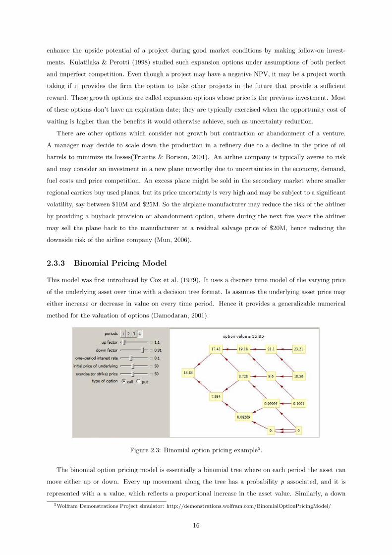
2.3.3 Binomial Pricing Model

This model was first introduced by Cox et al. (1979). It uses a discrete time model of the varying price

of the underlying asset over time with a decision tree format. Is assumes the underlying asset price may

either increase or decrease in value on every time period. Hence it provides a generalizable numerical

method for the valuation of options (Damodaran, 2001).

Figure 2.3: Binomial option pricing example5.

The binomial option pricing model is essentially a binomial tree where on each period the asset can

move either up or down. Every up movement along the tree has a probability p associated, and it is

represented with a u value, which reflects a proportional increase in the asset value. Similarly, a down

5Wolfram Demonstrations Project simulator: http://demonstrations.wolfram.com/BinomialOptionPricingModel/

16

movement along the tree has the 1-p probability associated and it is represented with a d value, which

instead reflects a proportional decrease on the asset value and depends on u: d = 1/u. Once we reach the

maturity date and calculate the final period, the probability distribution of the corresponding outcomes

can be calculated (Oliveira, 2012). If the binomial process has multiple periods, the valuation must

proceed iteratively starting from the last period and moving backwards in time until the current point in

time.

In order to calculate the value of a call option we need to work backwards through the tree starting

with the known final option values. By recognizing that it is always possible to create a replicating

portfolio based on the risk-neutral solution, under the assumption of no-arbitrage, this portfolio must

have the same value as the option. Having the risk-free rate r and time to maturity T, the value of the

asset A will be:

A = [p ∗Au+ (1− p) ∗Ad] ∗ e−rT (2.5)

We can then find the risk neutral probability p:

p =A ∗ erT −AdAu−Ad

(2.6)

The resulting p is the probability of the asset A increasing in value to Au, and 1-p the probability of

decreasing to Ad. Furthermore, using the strike price X of the option we can then calculate the value

of the call option. A risk neutral assessment gives a probability p of earning the difference between the

asset value and the strike price, and a probability 1-p of earning 0.00$. Hence, we can calculate the value

of the call option C with the following expression:

C = [p ∗ (Au−X) + (1− p) ∗ 0)] ∗ e−rT (2.7)

where C is the value of the call option, p is the risk neutral probability, X is the option’s strike

price, r is the risk-free rate and T represents the time to maturity. When we have more than one period

changes we wind up with more possible outcomes. The approach for solving this problem is basically

the same but has to be done iteratively, working backwards. The replicating portfolios are created at

each step and valued, providing the values for the option in that time period. The final output from

the binomial option pricing model is a statement of the value of the option in terms of the replicating

portfolio (Damodaran, 2001). The amount of values an asset can take over time is basically limitless.

The binomial method should be done with a large number of sub-periods so it gives a more realistic and

accurate view of the option’s value. As the number of intervals increases, the range of possible changes

in the value of the asset must be adjusted to keep the same standard deviation (Brealey & Myers, 2003).

Given a volatility estimate we can construct the price process with as many intervals as we want by

applying these equations:

u = eσ√h , d = 1/u (2.8)

where σ represents the volatility and h is the interval as fraction of year.

17

The binomial model helps us comprehend the determinants of option value. Its value is not determined

by the expected price of the asset, it is determined by its current price, which reflects expectations about

the future. If the option value deviates from the value of the replicating portfolio, it would turn into a

money machine. As an example, if the portfolio that replicates the call costs more than the call itself in

the market, one could buy the call, sell the replicating portfolio and be guaranteed the difference as profit.

This would be made without investment nor risk, and would deliver positive returns. The cash flows on

the two positions would offset each other, leading to no cash flows on subsequent periods (Damodaran,

2001).

2.3.4 Monte Carlo Simulation

The use of Monte Carlo in finance was first advocated by Hertz (1964) through his Harvard Business

Review article where he discussed its application in corporate finance. After more than a decade, Boyle

(1977) published his work on the use of simulation in derivative valuation for the first time. The Monte

Carlo Simulation is complementary to other numerical methods such as decision trees and finite differences

(Longstaff & Schwartz, 2001). It is, in its simplest form, a random number generator that is useful for

forecasting, estimation, and risk analysis (Mun, 2010). It uses numerous scenarios of a model that

converge to its real value due to the Law of Large Numbers. It’s a stochastic technique which relies on

the generation of random numbers and probability theory to derive a solution to the problem. Hence,

when the number of simulation tends to infinity, the standard deviation tends to zero (Boyle et al., 1997).

To calculate future cash flows and a project’s volatility using Monte Carlo Simulation we should start

by performing a sensitivity analysis. By setting the Net Present Value (NPV) of the project as a resulting

variable, we can change each of its input variables and see the change on the resulting NPV. These input

variables include revenues, costs, tax rates, discount rates, etc. By changing each of these input values by

a set amount and seeing the effect on the resulting NPV, we can trace the critical success drivers of the

model. These drivers are prime candidates for the Monte Carlo Simulation (Mun, 2010). Some of these

critical success drivers may be correlated, therefore a correlated simulation may be required (Brealey &

Myers, 2003).

By setting probability distributions on the critical input variables, we can calculate a distribution

of the project’s cash flows and the implied volatility. On each simulation, the variables get their values

selected randomly from their probability distribution functions, resulting in a corresponding cash flow

(Chandra, 2008). After enough simulations we can define a simulated distribution of these cash flows and

its implied volatility.

We can also use Monte Carlo to calculate volatility in real options analysis. In this case, the underlying

variable is the future profitability of the project, which is the future cash flow series. Its implied volatility

can be calculated through the results of the simulation. The volatility is typically measured as the

standard deviation of the logarithmic returns on the free cash flow stream (Mun, 2010).

Although the use of Monte Carlo on complex valuations is quite appealing, it requires a huge number

of simulations to provide reliable results. In fact, its standard deviation does not depend on the size of the

problem but on the number of simulations run. Boyle et al. (1997), Longstaff & Schwartz (2001) mention

18

more efficient ways of reducing the error by using the control variates approach and the antithetic variates

approach.

2.4 Phased Investment and Real Options

When considering an investment on a new technology based product it is hard to estimate its demand

due to a lack of historical data. Market studies can provide an idea about the size of the market and

its evolution, but this information is based on buying intentions. These intentions depend on their

surrounding circumstances and may not correspond to the reality once the product is commercialized.

When we undertake an investment based on market expectations we expose it to the risk of over-sizing or

under-sizing the production capacity. However, a phased investment approach allows for the distribution

of costs, which avoids irreversible losses if the demand’s evolution proves to be lackluster. Moreover,

an initial investment of a reduced size serves as a source of information about the market’s demand,

increasing the reliability of our growth estimates. In this way we can plan an expansion of a more

appropriate size.

In option valuation, the possibility of deferral provides two additional sources of value when compared

to the NPV. The first is the ability to pay later rather than sooner, since we can earn the time value

of money on the deferred expenditure. The second is the ability to observe the market conditions;

specifically, the value of the underlying asset may change. If the value of the underlying asset increases,

we can still acquire them simply by exercising our option. Yet if the value goes down, we can decide

not to acquire them. By waiting, we can avoid making a poor decision. In the end, we have maintained

the ability to profit from good outcomes and insulated ourselves from some bad ones. Traditional NPV

analysis misses the extra value associated with deferral because it assumes the decision cannot be put

off. In contrast, option pricing presumes the ability to defer and provides a way to quantify the value of

deferring (Luehrman, 1998).

The use of Real Options fits well in this type of valuation because it embodies the management

flexibility in project valuations (Trigeorgis, 1995). Real Options valuation always considers other possible

alternatives; invest now or delay the investment until better economic or technological conditions are

present; keep the project active or abandon it provided there is no other viable option. If we take into

account the irreversibility of some decisions and the limited time we have to execute them, these decisions

can be considered real options for the purpose of valuation (Brealey & Myers, 2003). Moreover, exercising

a decision over the alternative may represent a lost opportunity; if we invest now we lose the opportunity

to wait.

On an expansion perspective, any expansion decision of a determined size and time frame is char-

acterized by irreversibility and uncertainty. The expansion decision itself raises questions about its size

and time-frame. On one hand, delaying the decision too much implies foregoing future cash flows gen-

erated by the investment decision, allowing competition to take over or simply becoming technologically

outdated. On the other hand, the size of the investment should be big enough to cover the product’s

demand while avoiding an over-sized production output (Lopes, 2007). In short, the option to defer will

19

be more valuable while the uncertainty is excessively high. Following this line of thinking, investment in

a project that may not be profitable in its earlier stage may be justifiable if we take further investment

options into account. The expansion of the project may bring enough profit to offset the cost and turn

a project profitable as a whole, hence justifying the initial investment (Brealey & Myers, 2003).

While the seed investment estimates are based on expectations, future decisions may use the informa-

tion provided by this initial investment. The seed investment provides information, even if it’s partial,

about the stochastic critical values that drive the cash flows of the project expansion (Lopes, 2007). The

higher the initial investment, the bigger the sample will be, hence providing more accurate information.

Intuitively, the size of the sample depends on the seed investment value and so do the results from the

sample, although on a decreasing function. Once the seed investment is committed, information about

the market will start flowing in. This passive waiting for information represents a cost of opportunity.

By delaying the expansion decision in favor of information gathering, we forfeit those future cash flows

(Brealey & Myers, 2003). However, the information gathered may anticipate the decision to expand,

provided the estimated cash flows will offset the costs (Lopes, 2007).

20

Chapter 3

Methodological Approach to the

Case Study

3.1 The Net Present Value and Option Pricing

The Net Present Value is one of the traditional methods used in capital budgeting to analyze the prof-

itability of an investment. It can be described as the difference amount between the sums of discounted

cash inflows R and outflows C, discounted to their present value using the minimum acceptable rate of

return r established for the project. The following NPV formula accommodates the spread of costs of

projects for n years:

NPV = −n∑t=1

Ct(1 + rt)t

+

n∑t=1

Rt(1 + rt)t

(3.1)

where Ct represents the outflows, Rt represents the cash inflows, rt is the minimum acceptable rate

of return for the project and t represents the time in years. We can assume from this formula that the

Net Present Value of an investment will only be positive when the sum of all cash flows, discounted to

present value, are positive. A proposed investment will only be economically acceptable if its NPV is

greater than zero. Having an investment where its NPV is zero means the initial investment would return

itself with its present value in n years, and should only be done based on other criteria, e.g., strategic

positioning or other factors not explicitly included in the calculation.

The NPV method may be used to choose between concurrent projects, where a higher NPV provides

a greater value from the investment. Alternatively, it can also be used to minimize costs by choosing

concurring projects with the lowest absolute negative NPV value, when such projects must be chosen

(Oliveira, 2012). The success and accuracy of a DCF analysis depends on the choice of the accompanying

discount rate: if it is too high it might lead to the rejection of the project that could otherwise be

accepted. But if it is too low projects that should be rejected might be accepted due to a positive NPV

value (Mbolo, 2008).

21

On a real options analysis, when a final decision on a project can no longer be deferred its option has

reached its expiration date. Hence the time value of money and the riskiness of the project assets become

irrelevant for the decision. At that time, either the option value will be zero or it will be the difference

between the underlying asset and the strike price. So if the value of the project assets is the underlying

asset, and the expenditure required is the strike price, then according to equation 3.1 the NPV and the

option model will be the same at that time. From another perspective, if the NPV is zero that means

the corporation will not invest, so the project value is zero rather than negative (Luehrman, 1998).

3.2 Introduction to the Investment Models

Most Real Options models consider an investment as irreversible (Dixit & Pindyck, 1994; Brealey &

Myers, 2003), so the initial investment should avoid over-sizing the production capacity K. Although it

might be mathematically possible that the demand will satisfy a determined offer, there is always the

risk that the investment comes out of the product’s life-cycle. The investment function that defines the

cost of installing a determined production capacity K is:

I(K) = aK (3.2)

where a is the setup cost per unit. The stochastic variable θ represents the ratio between the product’s

demand D and the production capacity K, and will henceforth be called hedged capacity. Braumann

(2005) defines it as:

dθ

dt= αθdt+ σθdW (3.3)

where α is the market trend coefficient, σ is the standard deviation and dW represents increments on

a Wiener process. The revenue function for a determined hedged capacity θ can be written as:

R(θ,K) = pθK (3.4)

where p is the revenue from each unit produced, θ is the hedged capacity and K is the production

capacity. We can fit Lopes’ (2007) cost function G(θ,K) to our project valuation, where the first compo-

nent bθK represents the variable costs and the remaining components represent the fixed costs depending

on the production capacity:

G(θ,K) = bθK + cK +k

2K2, θ ≤ 1 (3.5)

where b is the cost per unit produced, c and k are fixed cost coefficients, K is the production capacity

and θ is the hedged capacity. Due to economies of scale, an increase in capacity should also increase costs

but decrease marginal costs. To assure this behavior, we must impose certain values for the coefficients:

b, c > 0 and k < 0. But these coefficients must also vary according to the production capacity so it

produces an economy of scale:

22

G(θ,K) =

bθK + c(1)K + k(1)

2 K2,

bθK + c(2)K + k(2)

2 K2,

bθK + c(n)K + k(n)

2 K2,

(3.6)

We can define our project’s annual cash flow equation Π(θ,K) = R(θ,K)−G(θ,K) as:

Π(θ,K) = pθK −(bθK + cK +

k

2K2

)= K

[mθ −

(c+

k

2K

)](3.7)

where m represents the margin per unit produced, c and k represent the fixed costs coefficients and θ

represents the hedged capacity. We will not consider depreciation of tangible assets. This model assigns

the initial volatility value based on the historical standard deviation of the market data, with adjustments

made according to the investment model. For instance, in the phased investment model the volatility

σp depends on the initial production capacity K0 and a minimum capacity Km necessary to retrieve

information about the market:

σ2p = σ2

h

(2− K0

Km

)(3.8)

where σh represents the historical volatility. Notwithstanding, if there is no seed investment, according

to equation 3.8 the initial volatility coefficient σs ends up being twice the historical volatility. However,

in order to define the phased investment volatility we first need to determine the minimum capacity Km

necessary to retrieve information about the market. A sample size typically depends on four things: the

population size, the confidence interval, the confidence level and worst acceptable frequency or standard

deviation. The confidence interval C determines how much higher or lower than the population mean

we are willing to let the sample mean fall. The confidence level represents how confident we want to be

that the actual mean falls within the confidence interval. Finally, the standard deviation represents the

variance in the behavior, the result farthest from the rate that we would accept in our sample:

N =Z2 ∗ σ ∗ (1− σ)

C2(3.9)

where N is the minimum sample size, Z is the Z-score for a given confidence level, C represents

the confidence interval and σ is the standard deviation in the behavior. But if we know the size of the

population, we can adjust the sample size with the following expression:

Km =N

1 +N − 1

K

(3.10)

The project’s expected rate of return ρ to be used in our methodological approach to the single invest-

ment model must be higher than the trend rate, otherwise waiting longer would always be a better policy

and the optimum would never exist and consequently the models would not have economic interpretation

(Dixit & Pindyck, 1994). Lopes (2007) suggests the use of a value greater than the trend coefficient plus

half the model’s variance to adjust for the risk:

23

ρ > α+σ2s

2(3.11)

where α is the project’s trend rate and σ2s is the single investment variance. Although it is possible to

use different values according to the investment model - since the phased investment model anticipates

the behavior of the market by applying the Kalman filter- we will use the same value to simplify the

comparison between the models before any investment is made.

Lastly, the project’s convenience yield δ will depend on the expected rate of return, the trend rate

and each model’s volatility (Lopes, 2007):

δ = ρ− α+σ2

2(3.12)

where δ represents the convenience yield, ρ is the expected rate of return, α is the trend rate and

σ2 is the variance in each model. However, in the case of the phased investment model, the convenience

yield will depend on the size of the seed investment. Furthermore, on the phased investment model with

the Kalman filter the convenience yield is constantly updated with the new information generated by the

seed investment.

3.3 Single Investment Model

Our single investment model is based on Dixit & Pindyck (1994)’s basic model. It assumes that the

timing of the investment and the production capacity to be installed K depends on the evolution of the

demand and an expected production capacity. Hence, the value of the project V (θs,K) depends on the

hedged capacity evolution θs and the production capacity K of the project. The optimal hedged capacity

θ∗s delineates the border between investment and deferral, and such decision can be assessed with the

option formula F (θs,K):

V (θs,K) = Π(θs,K)− I(K) , F (θs,K) = max[0, V (θs,K)] (3.13)

where θs represents the hedged capacity and K is the production capacity. We can valuate our invest-

ment option through dynamic programming; dynamic programming is a very general tool for dynamic

optimization, and is particularly useful in treating uncertainty. In this case, it breaks a whole sequence

of decisions into two components: the immediate decision, and a valuation function that encapsulates

the consequences of all subsequent decisions, starting with the position that results from the immediate

decision. By establishing a finite planning horizon, the very last decision at its end has nothing following

it, and can therefore be found using static optimization methods (Dixit & Pindyck, 1994). Using dynamic

programming, the value of the option may be calculated with the following expression:

F (θs,t,K) = max[E[e−ρdtF (θs,t+dt,K)

],Π(θs,t,K)− I(K)

](3.14)

where θs is the hedged capacity, K is the production capacity and ρ is the expected rate of return.

24

The valuation tests the expected present value of the option under the effect of the stochastic variable

θs, with the stopping boundary defined as the project’s cash flows and the investment cost: Π(θs,t,K)−

I(K). So the value of the option is given by:

F (θs,t,K) = E[e−ρdtF (θs,t+dt,K)

](3.15)

where θs is the hedged capacity, K is the production capacity and ρ is the expected rate of return.

But for a really small time interval dt, we can simplify the equation since eρdt ≈ 1 + ρdt:

eρdtF (θs,t,K) = E [F (θs,t+dt,K)] , (3.16)

ρF (θs,t,K) dt = E [dF (θs,t,K)]

where θs,t is the hedged capacity, K is the production capacity and ρ is the expected rate of return.

Hence, assuming our option F (θs,K) has no maturity date, we remove the variable of time. Since

dF (θs,K) is a stochastic process which depends on θs, we must apply Ito’s formula to expand the value

of the derivative. But the production capacity variable K depends on the manager’s decision, and it will

only vary when he decides to change it, therefore dK = 0 (Lopes, 2007). As a result, the Ito’s formula

for the expansion of the derivative can be written as:

dF (θs,K) =dF (θs,K)

dθsdθ +

1

2

d2F (θs,K)

dθ2s(θs)

2(3.17)

Excluding the derivative steps, we can simplify it to the following partial differential equation (PDE):

1

2σ2sθ

2s

∂2F (θs,K)

∂θ2s+ αθs

∂F (θs,K)

∂θs− ρF (θs,K) = 0 (3.18)

where σs is the volatility coefficient, θs is the hedged capacity, α is the trend coefficient and ρ is the

expected rate of return. The expected rate of return must satisfy the condition ρ > α+ σ2s/2 or else the

model won’t have economic interpretation (Dixit & Pindyck, 1994; Lopes, 2007).

The PDE allows us to determine the value of the option but it has the following restrictions: the first

restriction (equation 3.19) assents there is no investment decision if there is no demand:

F (0,K) = 0 (3.19)

The second restriction (equation 3.20) represents the optimal investment: the exercise of the invest-

ment option. Its value F (θ∗s ,K) is equal to the project value V (θ∗s ,K) and can be represented as:

F (θ∗s ,K) = Π(θ∗s ,K)− I(K) (3.20)

The third restriction (equation 3.21) limits the value of the project to its production capacity since

the company cannot sell more than it produces (Bar-Ilan & Strange, 2000):

25

limθs→∞

F (θs,K) = Π(1,K)− I(K) (3.21)

The fourth restriction (equation 3.22) states there is only one value for θ∗s , and any other value cannot

be the optimal:

∂F (θ∗s ,K)

∂θs=∂Π(θ∗s ,K)

∂θs(3.22)

The last restriction (equation 3.23) determines the maximum value for the production capacity, where

any revenue from a unit produced is equal to its investment cost:

∂Π(θs,K∗)

∂K∗=dI(K∗)

dK∗(3.23)

Going back to the determination of the option’s value, equation 3.18 is a partial differential equation

which depends on the option value F (θs,K) and its respective derivatives, and whose general solution is

(Dixit & Pindyck, 1994) F (θs,K) = Aθβss . Applying the general solution to our PDE (3.18), excluding

the derivative steps, we can also represent it as:

F (θs,K)

(1

2σ2sβs (βs − 1) + αβs − ρ

)= 0 (3.24)

which has two possible results, either F (θs,K) = 0 or

(1

2σ2sβs (βs − 1) + αβs − ρ

)= 0 (3.25)

So the solution of the PDE rests upon the the parameter βs, which, by application of the quadratic

formula, has two roots:

βs,1 =1

2− α

σ2s

+

√(α

σ2s

− 1

2

)2

+2ρ

σ2s

(3.26)

βs,2 =1

2− α

σ2s

−

√(α

σ2s

− 1

2

)2

+2ρ

σ2s

where α is the trend rate, σ2s is the variance and ρ is the expected rate of return. Hence, the general

solution may be divided in two components (Dixit & Pindyck, 1994):

F (θs,K) = A1θβs,1s +Asθ

βs,2s (3.27)

However, the expected rate of return ρ and the variance σs are necessarily positive, so one root is

positive (βs,1) while the other is negative (βs,2). Since the first restriction (equation 3.19) A2 is equal to

null, only the positive root, henceforth represented as βs, will be used for the option valuation:

F (θs,K) = A1θβss (3.28)

26

where θs represents the hedged capacity, K is the production capacity and βs is the solution to the

quadratic PDE. The option derivative is:

dF (θs,K)

dθs= βsA

βs−11 (3.29)

and applying the fourth restriction (equation 3.22) which states that there’s only one optimal value

for the hedged capacity θs, we have:

A1 =

dΠ (θs,K)

dθs

β1 (θ∗s)βs−1 (3.30)

Using equations 3.20, 3.28 and 3.30 we can now define the expression that determines the optimal

hedged capacity θ∗s :

dΠ (θs,K)

dθs

βs (θ∗s)βs−1 ) (θ∗s)

βs = Π (θ∗s ,K)− I (K) (3.31)

where θs os the hedged capacity, K represents the production capacity and βs is the solution to the

PDE. Yet we still need to determine the expected value of the cash flows. The expected present value of

the discounted cash flows can be represented as:

E [Π(θs,K)] =

∫ ∞0

K

[mE [θs]−

(c+

k

2K

)]e−ρsds (3.32)

where K is the production capacity installed, m is the margin per unit produced, c and k are fixed

cost coefficients, ρ is the expected rate of return and θs represents the hedged capacity. Hence, the

expected value of Π (θ∗s ,K) when the initial moment is t∗:

E [Π(θs,K)] = K

[mθ∗sδs−(

2c+ kK

2ρ

)](3.33)

where m is the margin per unit, θ∗s is the optimal hedged capacity, δs is the convenience yield, c and

k are fixed cost function coefficients, ρ is the expected rate of return and a is the setup cost per unit.

The convenience yield is the difference between the expected rate of return and the trend rate plus half

its variance (Lopes, 2007; Dixit & Pindyck, 1994):

(δs = ρ− α+

σ2s

2

)(3.34)

Hence, the derivatives of the expected present value of the discounted cash flows at time t∗ are:

dΠ (θs,K)

dθs=mK

δs(3.35)

dΠ (θs,K)

dKθs= −c+ kK

ρ(3.36)

Finally, the optimal hedged capacity value θ∗s can be calculated with equations 3.35, 3.33, 3.2 and

27

3.31:

θ∗s =βs

βs − 1

δsm

(2c+ kK

2ρ+ a

)(3.37)

where βs is the positive root of the quadratic PDE (4.9), δs is the convenience yield, m is the margin

per unit, c and k are fixed cost function coefficients, ρ is the expected rate of return and a is the setup

cost per unit. Once we have the optimal value of the hedged capacity θ∗s , we can determine its the

expected value for the moment of first passage (Ingersoll, 1987):

E [T ∗] =

ln

(θ∗sθ0

)α− σ2

s

2

,σ2s

2> 0 (3.38)

where θ0 is the initial value of the hedged capacity at the start of valuation, α is the trend coefficient

and σ2s is the variance. We can also use θ∗s to find the value of the project V (θ∗s ,K):

V (θ∗s ,K) =βs

βs − 1K

(2(c+ ρa) + kK

2ρβs

)(3.39)

where βs is the positive root of the quadratic PDE (x), c and k are fixed cost coefficients, ρ is the

expected rate of return and a is the setup cost per unit. We can now represent the investment option

value in this model Fs(θs,K):

Fs(θs,K) =

mK

βsδsθs ifθs ≤ θ∗s

K

[mθsδs−(

2c+ kK

2ρ+ a

)]ifθs ≥ θ∗s

(3.40)

where m is the margin per unit, K is the production capacity, βs is the solution of the PDE, θ is the

hedged capacity, c and k are fixed cost coefficients, ρ is the expected rate of return, a is the setup cost

per unit and δs is the convenience yield. For any θs lower than the optimal θ∗s , the option value is given

by the possibility of investment; but when θs is higher the option value will be that of the project after

investment, minus costs of investment (Lopes, 2007).

3.4 Two-Phased Investment Model

Our phased investment model has two components: a seed investment and an expansion phase. The

expansion phase can be considered an option to expand Fp whose price is the initial investment (Dixit

& Pindyck, 1994). Trigeorgis (1995), Kulatilaka & Perotti (1998) argue that the seed investment project

does not necessarily needs to be profitable if it eventually leads to follow-up investments that have positive

results, essentially meaning that those options increase the value of the investment. Since the value of

the seed investment is V0, the expanded project can be defined as Vp = V0 + Fp, therefore:

28

Fp = Vp − V0 ⇔ Fp(θp,K) =

0 θp = 0

E [Fp(θp,dt,K)− V0] 0 < θp ≤ θ∗p

Π(θp,K)−Π(1,K0)− I(K −K0) θp ≥ θ∗p

(3.41)

where K0 is the production capacity installed by the seed investment, K is the expected production

capacity and θp is the hedged capacity in this model. The seed investment can be used as a source of

information about the market, hence reducing its volatility. However, the initial production capacity K0

must be big enough to provide information with a desired level of significance. According to Newbold

et al. (2007) the test of the average value on a Normal distribution with unknown variance can be done

with the statistic t-student distribution:

θp − θpsθp√K0

< −tK0−1,αs; θp = α−

s2θp2

(3.42)

where θp is the observed mean of the sample, θp represents the test value, sθp the standard deviation of

the sample, K0 is the initial production capacity and αs represents the level of significance. But θp includes

the variance, hence the minimum size of the sample must also validate the hypothesis regarding the

variance used in the model (Newbold et al., 2007). To this end we can use the Chi-Squared distribution:

(K0 − 1)s2θpσ2p

> χ2K0−1,αs

(3.43)

where K0 is the initial production capacity, σ20 is the variance used for the test of the hypothesis, s2θp

the variance of the sample and αs represents the level of significance.

Going back to the option valuation, equation (3.41) has three possible results: the first means the

expansion option has no value and therefore it is abandoned. In such case the expansion would not

happen so the value of the project remains the same. The second result expresses the need to wait more

time for the evolution of the hedged capacity variable since it has not reached its optimal value; and the

third represents the exercise of the expansion option (Lopes, 2007). As in the single investment model,

we can use the option formula:

Fp = max[0, e−ρdtE [Fp − V0] ,Π(θp,K)−Π(1,K)− I(K −K0)

](3.44)

where ρ is the expected rate of return, θp is the hedged capacity, K0 is the production capacity and K

is the expected production capacity after expansion. As in the single investment model, we assume there

is no maturity date. As a result we can rewrite the equation as: ρFp(θp,K)dt = E [dFp(θp,K)− V0dt],

and its resulting partial differential equation (PDE):

1

2σ2θ2p

∂2Fp(θp,K)

∂θ2p+ αθp

∂Fp(θp,K)

∂θp− ρFp(θp,K) = 0 (3.45)

where σ∗p is the variance in this model, θp is the hedged capacity, α is the trend coefficient and ρ

29

represents the expected rate of return. The above PDE has the following restrictions: the first is defined

in the same as in the single investment model (equation 3.19) and assents there is no value in the expansion

option if there is no demand. The second restriction (equation 3.46) states that the expansion option has

the same value as the project and therefore the investment decision can be taken:

Fp(θ∗p,K) = Π(θ∗p,K)−Π(1,K0)− I(K −K0) (3.46)

The third restriction (equation 3.47) limits the value of the option regardless of the demand, since

the number of units sold cannot exceed the production capacity:

limθp→∞

Fp(θp,K) = Π(1,K −K0)− I(K −K0) (3.47)

The fourth restriction is also defined in the same as in the single investment model (equation 3.22).

It guarantees θ∗p is the optimal value for the exertion of the option; if the company decides to defer the

investment, it will forfeit cash flows with greater value. The last restriction (equation 3.48) determines

the maximum value of the production capacity, where any revenue from a unit produced is equal to its

cost:

∂Π(θ∗,K)

∂K=∂I(K −K0)

∂K(3.48)

The following equations are the same as in the single investment model:

Fx (θp,K) = A1θβpp (3.49)

δp = ρ− α+σ2p

2(3.50)

βp =1

2− α

σ2p

+

√(α

σ2p

− 1

2

)2

+2ρ

σ2p

(3.51)

dΠ (θp,K)

dθp=mK

δp(3.52)

dΠ (θp,K)

dKθp= −c+ kK

ρ(3.53)

Excluding the derivative steps for the calculation of the optimal value of the hedged capacity θ∗p:

θ∗p =βp

βp − 1

δpmK

[K

(2c+ kK

2ρ+ a

)+K0

(2(m− c)− kK0

2ρ+ a

)](3.54)

where βp is the positive solution of the quadratic PDE (equation 3.45), δp is the convenience yield,

m is the margin per unit, c and k are fixed cost coefficients, a represents the setup cost per unit, ρ is

the expected rate of return and K0 is the production capacity installed with the seed investment. We

can clearly see the difference between this equation and its equivalent from the Single Investment Model

(equation 3.37): the contribution from the seed investment to the determination of the optimal value.

Once we have found the optimal value θ∗p we can determine its expected value for the first passage

30

with Ingersoll’s equation (equation 3.38). Furthermore, we can now represent the value of the option to

expand Fp(θp,K):

Fp(θp,K) =

0 θp ≤ 0

mK

βpδpθp 0 ≤ θp ≤ θ∗p

K

(mθpδθp− 2c+ kK

2ρ

)−K0

2(m− c)− kK0

2ρ− a(K −K0) θp ≥ θ∗p

(3.55)

where m is the margin per unit, βp is the positive solution of the quadratic PDE (x), δp is the

convenience yield, θp is the hedged capacity, c and k are fixed cost function coefficients, ρ is the expected

rate of return, a represents the setup cost per unit and K0 is the production capacity installed with the

seed investment. In conclusion, the valuation of the Phased Investment Model ends up being similar to

the Single Investment Model. However, the seed investment has effects on the volatility coefficient which

ends up affecting the optimal value of the hedged capacity θ∗p.

3.5 Two-Phased Investment Model With Kalman Filter

The Phased Investment Model has the advantage of being able to retrieve information about the stochastic

variable evolution. The seed investment is, by definition, a small investment that provides a foothold on

the market. It does not cover the whole market, but it still provides partial information from the sample

of population. We can use this information to estimate the trend value α and the noise σdW, by filtering

the demand value according to the observed process (Lopes, 2007).

The Kalman filter is a set of mathematical equations that provides an efficient computational recursive

solution of the least-squares method. The filter supports estimations of past, present, and even future

states, and it can do so even when the precise nature of the modeled system is unknown (Bishop & Welch,

2001). This model aims to update the estimates of parameters when in presence of historical data. Each

current estimation depends on the Kalman Gain, a measured value and the previous estimation. With

this information we can try to eliminate the noise. Nevertheless, the Kalman filter inputs are data from

a sample and not from the global market itself. Still, it is statistically possible to determine what size

the sample must have to provide values with an acceptable confidence interval (Newbold et al., 2007).

Remembering the equation of the stochastic variable θ with a time factor:

dθt = αθtdt+ σθtdWt (3.56)

The stochastic variable θ estimate in time t obtained from its initial value can be defined as:

θt = θaexp

(α− 1

2σ2

)(t− a) + σ (Wt −Wa)

(3.57)

The seed investment allows us to obtain an observed value H at moment t with a similar behavior:

31

Ht = µθt + ξtεt (3.58)

where εt represents the white noise, µ represents the average of the observations, and ξt represents

the standard deviation of the observations. Using historical data from the observed demand values, we

can define the representative function of the cumulative observations as:

Zt =

∫ t

0

Hsds (3.59)

Since Zt expresses the behavior of a stochastic variable it can also be expressed as:

dZt = µθtdt+ ξdXt (3.60)

where dXt represents increments in a Wiener process independent from dWt.

Seeing that both θ and Z are Gaussian processes, each random variable has a normal distribution.

In fθ(Z[0, t]) we have a normal distribution which we can use to estimate θ according to its expected

behavior and the registered observations:

θt = E [θt | Z [0, t]] (3.61)

and variance:

St = E[(θt − θt)2 | Z[0, t]

](3.62)

The Kalman Filter uses a closed system of dynamic equations to determine values for both ϕt and St

through an optimal filter(Liptser & Shiryayev, 2001):

dθt = αθtdt+µ

ξ2tStθt (dZt − µθtdt) (3.63)

dStdt

= 2αSt −µ2

ξ2tS2t + σ2 (3.64)

Since both θ and Z are Gaussian processes, their conditional distributions are Normal. Our goal is

to estimate the values for θ and the conditional variance S according to their expected behavior and the

registered observations. To do so we use a closed system of dynamic equations which define an optimal

filter (Liptser & Shiryayev, 2001):

dθt = αθtdt+µ

ξtStθtdXt (3.65)

where θt represents the current estimation and dXt an increment of a Wiener process, and:

Stdt

= 2αSt −µ2

ξ2tS2t + σ2 (3.66)

32

Equation 3.65 is the measure equation and represents the update of the estimate θ after the incor-

poration of the information present in Zt. In other words, the estimated θ is the previous estimation

modified by the new information. Equation 3.66 weights the new information against the historical data

and represents the effect of a learning behavior by allowing an increase in precision through time (Epstein

et al., 1999). Since there’s a change in the behavior of the stochastic variable that represents the hedged

capacity when we apply the Kalman filter, the representation of its optimal value θ∗k must be changed to

reflect these changes:

θ∗k =βk

βk − 1

ρ− α+ 12µ2

ξ2tS2t

mK

[K

(2c+ kK

2ρ+ a

)+ V0

](3.67)

where βk is the positive solution of the quadratic PDE, ρ is the expected rate of return, α is the trend

coefficient, m represents the margin per unit, c and k are fixed cost coefficients, V0 is the value of the

seed investment project and St is the conditional variance. Once we’ve found the optimal value θ∗k we

can determine its expected value for the first passage with equation 3.38.

Excluding the derivative steps, the conditional variance St can be represented as:

St =1

3St−1 +

2

3ξ2tα

µ2(3.68)

The above equation shows us St is constructed as a weighted average between the previous St−1

value and the last registered observation adjusted by a correction factor. If the trend values α and µ are

correctly estimated, they will have the same value, and their correction factor will be the inverse of the

trend coefficient.

33

34

Chapter 4

Case Study Analysis and

Description: Paydiant

4.1 Payment Industry Evolution and Paydiant

Paydiant is a start-up technology based company from the United States that has created a white label

mobile wallet and payment solution (Alvarez et al., 2011). It allows banks, retailers and payment proces-

sors to deploy a branded contactless mobile wallet, a mobile payment and cash access platform without

involving new intermediaries nor hardware.

Paydiant’s prototype system consists of a software solution. Unlike NFC1 hardware alternatives,

customers just need to enroll their mobile phone electronic serial number and payment credentials in a

secure Paydiant website and then download a free Paydiant app. For the merchants, they only need to

acquire the software and load it onto existing POS systems. Then the software enables the display of

a two-dimensional barcode used in the transaction processing. To illustrate the transaction process, a

consumer enters his PIN to unlock his smartphone, then opens the Paydiant’s app and chooses the ”pay

in store” button. The cashier prompts a mobile transaction and the LCD displays Paydiant’s unique 2-D

barcode. The customer scans it using the smartphone camera. Up that time, the transaction is processed

through the system and applies for credit from the loyalty programs. Afterwards the phone displays the

total purchase amount and the customer selects which of the preloaded payment credentials he would

like to use. Finally, the purchase is confirmed by the consumer and once the transaction is complete, an

e-receipt is displayed on their phone (Alvarez et al., 2011).

The evolution of the POS2 systems such as Paydiant’s provides some advantages over the previous

systems. One advantage is the faster processing of a transaction, such as, when a consumer has to present

both credit card and the loyalty card. Another advantage is the added security at no additional cost,

since the customer no longer has to swipe his credit card. Finally there’s the advantage of not having to

1Near Field Communication (NFC) is a short-range high frequency wireless communication technology which enablesthe exchange of data between devices over about a ten centimeter distance. The technology is a simple extension of theISO 14443 proximity-card standard that combines the interface of a smartcard and a reader into a single device.

2Point of Sale, it refers to the physical location where an offline transaction occurs, which is oftentimes a retail shop orthe checkout counter in that shop.

35

carry around a wallet stuffed with cards, money, offers, coupons, etc3.

Considering this company is located in the U.S.A., it makes sense using data from the same location

for describing the history and evolution of its market. Electronic payment systems in the 20th century

consisted primarily on magnetic stripe cards, enabling consumers to pay on credit and debit cards.

These cards allow consumers to pay for their purchases using funds from their bank accounts. With

the emergence of the internet some other electronic payment forms started to appear, like PayPal and

Neteller, which use credit card information for transactions.

According to the Federal Reserve Bank of Boston (FRBB) magnetic stripe cards and other electronic

payments have been replacing checks in US non-cash payments. The number of US check payments by

all sectors (household, business and government) have been on the decline since 1996, where it amounted

for 50 billion per year, to around 25 billion payments in 2009. During the first decade of the XXI

century, debit card usage had grown significantly faster than credit cards, surpassing them by 2006.

Debit card payments increased more than fourfold since the year 2000, toppling check payments and

amounting for more than 38 billion in 20094. Credit cards also started increasing but remained steady

from 2006. Furthermore, available data shows that electronic payments, such as Automated Clearing

House, almost doubled in the same time frame, amounting around 19 billion payments (FRBB, 2012).

Table 4.1 confirms that issue, showing similar results: a decrease in check and cash usage, and an increase

in electronic account deduction, online bill payments, and magnetic cards.

Actual (2005-2008) Decreased Increased MaintainedCash 43.0% 16.0% 41.0%Checks 51.6 8.3 40.1Debit cards 17.3 49.5 33.2Credit cards 28.5 34.2 37.3Prepaid cards 28.7 14.1 57.2Electronic account deduction 14.0 42.6 43.4Online bill payments 10.3 60.6 29.1

Table 4.1: 2008 survey of consumer payment choice. Adapted from Foster et al, 2010.

In 2009, four companies owned the electronic payments system in the United States: Visa, Master-

Card, American Express and Discover. Together they had 631 million credit cards in circulation. Each

of these companies had created its own network through which its cards operated. Each of these brands

acted as their own card association, developing the operating procedures and rules for the issuance, use

and acceptance of their cards. These cards have fees associated to, which vary depending on their issuer

and how they are used. Debit cards are much like electronic checks, they are linked to the consumer’s

bank account. There are two types of debit cards in the US: signature debit and PIN debit cards, each

with their own rules. To further complicate, some cards combine credit and debit, some can be used in

ATM5, etc.(Alvarez et al., 2011).

The Federal Reserve Bank of Boston points to a significantly faster growth of debit card usage against

3Credit Union Journal, ’Consumers Ready to Swipe Their Phones’, January 2011.4The Wall Street Journal, ’Debit Cards: Think Before You Swipe’, September 2010.5Automated Teller Machine or cash machine.

36

credit cards (FRBB, 2012). While credit cards had their own networks created by the major credit card

brands, PIN debit cards worked on different networks. Many early debit cards were issued by banks

that also issued ATM cards, and these ATM cards operated on electronic funds transfer (EFT) networks.

These early EFT networks were created independently from the credit card networks and had different

ownership, operations and fees. In 2010, leading EFT networks included Interlink, Maestro, STAR,

NYCE, Pulse and ACCEL. Only STAR, NYCE and ACCEL were independent from the major credit

card competitors6.

In terms of payment instruments market share, table 3.2 shows an increase in both card and other

electronic payment systems and a decrease in paper payments from 2005 to 2010. The substitution of

checks by magnetic cards is one of the reasons pointed by the Federal Reserve Bank of Boston (FRBB,

2012).

2005 2010Volume Share Trans. Share Volume Share Trans. Share

Paper 3,417.08 50.45% 77.52 58.52% 3,086.28 38.97% 67.92 44.92%Checks 1,897.11 28.01% 26.06 19.6% 1,433.68 18.23% 16.98 11.24%Cash 1,401.68 20.69% 50.48 38.11% 1,539.17 19.43% 50.12 33.17%Money Orders 87.70 1.29% 0.77 0.58% 77.20 0.97% 0.65 0.43%Official Checks 24.92 0.37% 0.14 0.11% 21.79 0.28% 0.13 0.08%Travelers Checks 5.67 0.08% 0.08 0.06% 4.43 0.06% 0.05 0.03%Cards 2,707.62 39.98% 49.27 37.19% 3,811.30 48.12% 74.14 49.07%

Credit 1,708.39 25.22% 22.18 16.74% 1,942.26 24.52% 23.19 15.35%Debit 859.57 12.69% 22.08 16.67% 1,630.10 20.58% 43.52 28.81%Prepaid 111.31 1.64% 3.94 2.98% 172.36 2.18% 5.13 3.39%EBT Cards 28.36 0.42% 1.06 0.80% 66.58 0.84% 2.30 1.52%Electronic 648.50 9.57% 5.68 4.29% 1,022.43 12.91% 9.02 5.97%Preauthorized 381.70 5.64% 3.27 2.47% 521.78 6.59% 4.28 2.83%Remote 266.79 3.94% 2.41 1.82% 500.65 6.32% 4.74 3.14%TOTAL 6,773.20 100% 132.47 100% 7,920.00 100% 151.9 100%

Table 4.2: United States consumer payment systems, dollar volume and transactions in billions. Source:The Nilson Report. Issue 985, December, 2011.

The state of electronic payment systems such as debit and credit cards is relevant because a mobile

proximity payment system such as Paydiant’s typically uses these instruments for processing transactions.

Before the Internet, North American buyers would place orders via phone from home for products

they’d see on television or catalogs. With the emergence of the Internet the so called e-commerce started

to appear, and has been growing since. According to the Internet World Stats7 as of June, 2012 North

America region has the highest internet penetration (78.6%) worldwide, followed by Europe (63.2%), an

indispensable factor for the growth of e-commerce.

Retailers introduced e-commerce as a new segment in their business, each with their own offers to

bring in customers. The widespread Internet access and these offers prompted consumers to increasingly

shop online. As a result, in the US there were 163.1 million online payments in 2009, followed by 167.3

million in 2010 and 194.3 million in 2011. The consumer’s expanding ability to go online not only from

home or work, but from their cellphones, tablets, consoles, television sets or other devices also facilitates

6Pulse. ’The Evolution of US EFT Networks - Lessons to be Learned’.7Internet World Stats. ’World Internet Users and Population Stats’, accessed January, 2013.

37

the growth of e-commerce. Mobile commerce, or m-commerce, is expected to make up a larger share than

they have in the past, possibly accounting for one quarter of all e-commerce transactions (Bel & Gaza,

2012).

The use of smartphones has been steadily growing in the past years, surpassing the use of feature

phones in January 2012 (see Figure 4.1). By February 2013 around 133.7 million people in the US

owned smartphones, representing a 57% market penetration8. These phones have become of extreme

importance to their users, allowing them to surf the web and check emails, socializing, shopping and

check their banking accounts (Alvarez et al., 2011). According to a survey from Carlisle & Gallagher

Consulting Group, 48% of US consumers are interested in using a mobile phone wallet. Some of the

incentives go from lower interest rates and cash-back rewards to discounts and loyalty programs, and

the ability to track offers on their devices. Having to carry a number of cards for the purpose of loyalty

programs, and keeping track of terms and conditions is said to be frustrating9. Simultaneously, banking

and shopping apps is on the rise with 53 percent of American smartphone owners as regular users. In

addition, mobile shopping is rising with 30 percent of smartphone users already doing so10.

Figure 4.1: U.S.A. mobile phone subscribers by device, adapted from Alvarez et al. (2011).

Combining a mobile phone with computer and Internet capabilities brought in a host of new uses

for them. By incorporating new features such as GPS, it allowed users to find local merchants, and

local merchants to advertise to nearby smartphone users. Smartphones run on their own operating

systems which allow software developers to create software applications for them. These apps provide

smartphones many other capabilities, such as games, social networking, mobile banking, etc. Nowadays,

users can download apps for a variety of activities, customizing their phones to their own needs.

Online and offline checkout experiences are evolving, with technological innovations allowing new ser-

8comScore. ’February 2013 US Smartphone Subscriber Market Share’.9NFCNews. ’48% of US consumers want mobile wallet’, June, 2012.

10Nielsen. ’The Mobile Consumer’, 2013.

38

vices and solutions to be integrated, either online or at the counter. The payment interaction is becoming

a connection between the merchant and the customer, where loyal customers are being recognized and

rewarded for coming back, and new customers are offered comeback discounts. In North America, an

abundance of initiatives have been launched by various different players, such as banks, startups and

corporates, to provide these new services to merchants. Card schemes have been placing big bets and

money on marketing campaigns around the benefits of NFC, but have so far failed to reach critical mass.

Other players, such as Paydiant, are focusing on exploiting different technologies, such as the ubiquitous

internet connection, to enable mobile payment methods(Longoni & Gaza, 20123).

The use of the mobile phone for completing transactions has had and will continue to have a disruptive

effect in the payment industry, both on emerging and developed economies. In Kenya, the M-PESA is

solving liquidity problems of entire rural villages, where an average of 150M Ksh (e1.39M) is transferred

through M-PESA per day, although most of it is done in small amounts of around 1500Ksh (e13.93) per

transaction. In contrast, in the U.S.A square is affecting the POS market for small merchants, processing

more than $15 billion in payments on an annualized basis11.

It’s worth mentioning that Paydiant faces strong competitors in its market. Global internet giants

of the likes of PayPal, Google and Amazon, as well as the card networks, are testing new propositions.

PayPal is determined to hold on to its dominant position as dedicated online payments provider, while

also expanding the more traditional payment systems with magnetic stripe cards (Bel & Gaza, 2012). In

August 2012 PayPal announced a partnership with Discover, allowing it access to more than 7 million

vendors by swiping their cards on dongles. Moreover, PayPal is also working on its mobile wallet which

had already signed up eighteen thousand vendors by the end of 201212.

While giants battle for their market share, young innovators develop new mobile payment methods.

To list a few, Jumio and Card.io use computer vision technology to scan credit cards with the device’s

webcam to make payments13. MasterCard is working on a private-labeled wallet based on NFC and QR

code technologies. Similarly, Visa is betting on NFC and partnering with Samsung for its wallet to be

incorporated into all future mobile phones. Square, PayPal and iZettle offer free mobile card readers to

retailers and charge a percentage per transaction. Incidentally, Google, Paypal and Square are working

on wallet apps to allow its customers to pay with their own mobiles14. Paydiant, on the other hand,

offers a white label mobile wallet and payment solution to banks, retailers and credit card processors,

allowing them to use their own brands and create the opportunity of new revenue streams from highly

targeted mobile ads and offers (Alvarez et al., 2011).

Paydiant has been able to attract some big name partners and customers so far. It offers the platform

to ISOs and their sales partners through an arrangement with Vantiv. Paydiant also partnered with

outsourcing giant Fidelity National Information Services. FIS is the world’s largest global provider

dedicated to banking and payments technologies, serving more than 14 thousand institutions in over a

hundred countries. Other partners include pcAmerica, the Bank of America and Menusoft Systems.

11Square offers a card-reader which allows the swiping of debit and credit cards on smartphones or tablets12Mobile Entertainment, ’PayPal takes mobile wallet to more US retailers’, January 2013.13Payvision. ’Mobile Payment: a Shifting Landscape’, accessed January, 2013.14New York Times. ’Starbucks and Square to Team Up’, accessed March, 2013.

39

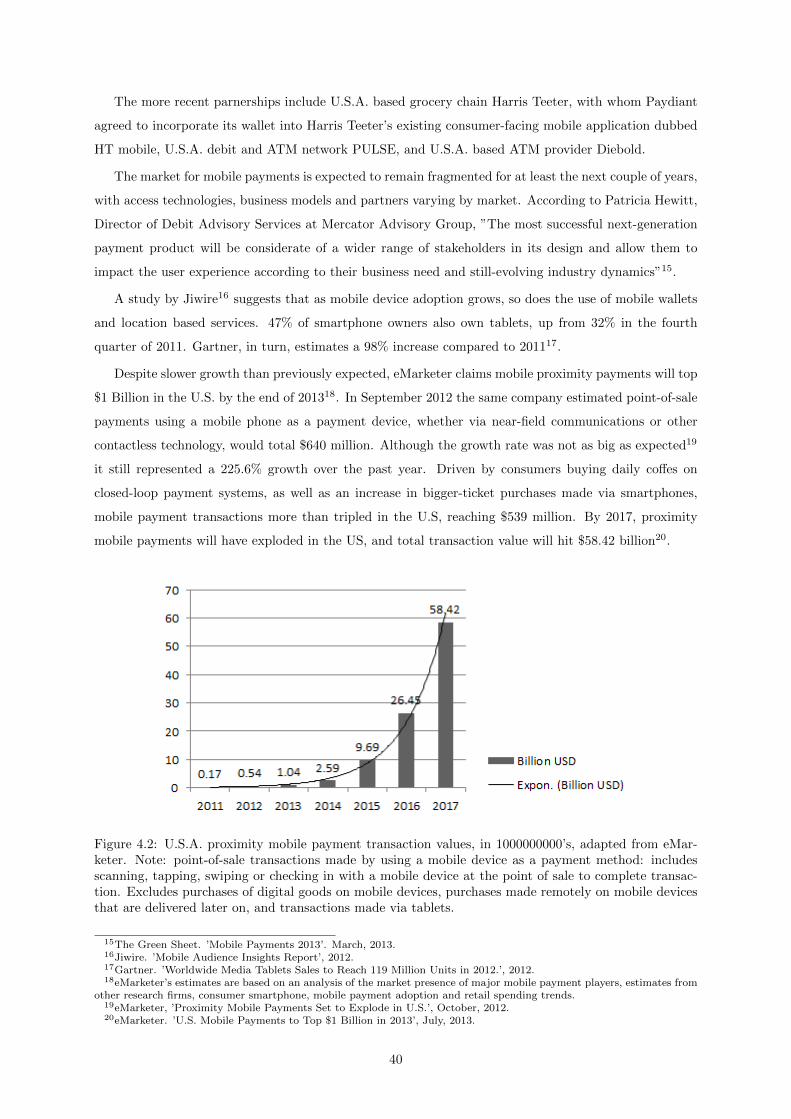
The more recent parnerships include U.S.A. based grocery chain Harris Teeter, with whom Paydiant

agreed to incorporate its wallet into Harris Teeter’s existing consumer-facing mobile application dubbed

HT mobile, U.S.A. debit and ATM network PULSE, and U.S.A. based ATM provider Diebold.

The market for mobile payments is expected to remain fragmented for at least the next couple of years,

with access technologies, business models and partners varying by market. According to Patricia Hewitt,

Director of Debit Advisory Services at Mercator Advisory Group, ”The most successful next-generation

payment product will be considerate of a wider range of stakeholders in its design and allow them to

impact the user experience according to their business need and still-evolving industry dynamics”15.

A study by Jiwire16 suggests that as mobile device adoption grows, so does the use of mobile wallets

and location based services. 47% of smartphone owners also own tablets, up from 32% in the fourth

quarter of 2011. Gartner, in turn, estimates a 98% increase compared to 201117.

Despite slower growth than previously expected, eMarketer claims mobile proximity payments will top

$1 Billion in the U.S. by the end of 201318. In September 2012 the same company estimated point-of-sale

payments using a mobile phone as a payment device, whether via near-field communications or other

contactless technology, would total $640 million. Although the growth rate was not as big as expected19

it still represented a 225.6% growth over the past year. Driven by consumers buying daily coffes on

closed-loop payment systems, as well as an increase in bigger-ticket purchases made via smartphones,

mobile payment transactions more than tripled in the U.S, reaching $539 million. By 2017, proximity

mobile payments will have exploded in the US, and total transaction value will hit $58.42 billion20.

Figure 4.2: U.S.A. proximity mobile payment transaction values, in 1000000000’s, adapted from eMar-keter. Note: point-of-sale transactions made by using a mobile device as a payment method: includesscanning, tapping, swiping or checking in with a mobile device at the point of sale to complete transac-tion. Excludes purchases of digital goods on mobile devices, purchases made remotely on mobile devicesthat are delivered later on, and transactions made via tablets.

15The Green Sheet. ’Mobile Payments 2013’. March, 2013.16Jiwire. ’Mobile Audience Insights Report’, 2012.17Gartner. ’Worldwide Media Tablets Sales to Reach 119 Million Units in 2012.’, 2012.18eMarketer’s estimates are based on an analysis of the market presence of major mobile payment players, estimates from

other research firms, consumer smartphone, mobile payment adoption and retail spending trends.19eMarketer, ’Proximity Mobile Payments Set to Explode in U.S.’, October, 2012.20eMarketer. ’U.S. Mobile Payments to Top $1 Billion in 2013’, July, 2013.

40

Still, the market is growing slower than formerly expected, as evidenced by eMarketer’s scaled back

estimates of user adoption and transaction value from initial projections in 2012. Numerous mobile wallet

initiatives are facing delays and adoption issues, as well as congested landscape of competing technologies,

which materially affected the outlook on mobile payment transaction values. Likewise, Gartner Inc also

scaled down its expectations, stating worldwide mobile payment transaction values will surpass $235.0

billion in 2013, an increase of 44.17% over 2012, and that it will exceed $720 Billion by 201721. Near Field

Communications’ (NFC) transaction value has been reduced by more than 40% throughout Gartner’s

forecast period due to disappointing adoption of NFC technology in all markets in 2012 and the fact that

some high-profile services, like Google Wallet and Isis, are struggling to gain traction.

Numerous forecasts attempt to quantify the global mobile payments industry, although estimates vary

widely based on the scope of what each research firm considers a mobile payment. Table 4.3 provides

comparative estimates of mobile payment transaction volume worldwide, from 2011 to 2017:

Source 2011 2012 2013 2014 2015 2016 2017Gartner, 2013 - $163.0 $235.0 - - - $721.0Yankee Group**, 2013 - - $60.7 $126.2 $230.3 $371.0 $531.2Gartner, 2012 $105.9 $171.5 - - - 617.0 -NPD In-Stat*, 2012 - $ 1.1 - - - $9.9 -IE Market Research, 2012 $47.2 - - - - $998.5 -Informa Telecoms & Media**, 2011 $2.4 - - - $71.0 - -Yankee Group**, 2012 - - - - - $366.7 -Juniper Research, 2012 - - - - - - $1,300.0

Table 4.3: Mobile transaction volume worldwide in billions. Note: * NFC/barcodes only, **NFC only.

4.2 Investment Assumptions

4.2.1 Expected Market Evolution

In order to quantify Paydiant’s market share we will use the values from eMarketer market study (figure

4.2) since it only includes proximity payments done via a mobile phone at the point of sale. It is also

important to mention that it only considers payments made in the U.S.A., which is where Paydiant

operates. Also, a recent market plan22 suggests Paydiant aims for a 10% market share.

Lint & Pennings (2001) and Kotler & Keller (2001) suggest an acceptable time for introduction of

four years for new products since they might become technologically outdated. Therefore, due to the

nature of our case study we will use data for the same period. Table 4.4 provides the expected yearly

growth rates for the period between 2011 and 2015:

Year 2012 2013 2014 2015% Change 217.647% 92.593% 149.038% 274.131%

Table 4.4: Proximity mobile payment forecast growth rates.

21Gartner, ’ Worldwide Mobile Payment Transaction Value to Surpass $235 Billion in 2013’, June, 2013.22University of Applied Sciences Amsterdam, ’Paydiant Mobile Playments Marketing Plan’, 2011.

41

Using the yearly growth rates based on eMarketer’s estimates from table 4.4 we can determine the

market trend rate α by calculating its geometric mean return: α = n√

(1 + r1) (1 + r2) · · · (1 + rn) − 1,

where n is the acceptable time for introduction for new technology products in years, r1 to rn represent

the expected yearly growth rates of each subsequent year after 2011, and α represents the compounded

annual trend rate. Therefore α is: 4√

(3.176) (1.926) (2.49) (3.741)− 1 = 1.747.

In order to quantify Paydiant’s operations we start by assuming the unit produced by Paydiant is a

processed transaction. Consequently, the production capacity represents the number of transactions the

Paydiant server can process. Each of these transactions have a value associated to, which may have wide

range of sizes depending on what a customer buys. A Starbucks coffee may represent a $5 transaction

while an opera concert ticket represents a $100 transaction. Using data from the magnetic strip card’s

industry, we calculated an average value for a transaction:

U.S. Dollars Market Share No. Transactions Market Share(1000000000’s) % (1000000000’s) %

Debit 1630.1 43.53 43.52 60.58Credit 1942.26 51.87 23.19 32.28Prepaid 172.36 4.60 5.13 7.14

Table 4.5: U.S.A. debit, credit and prepaid cards market data.

By dividing the dollar amount of each type of magnetic stripe card by their respective number of

transactions, we estimated an average value for debit, credit and prepaid cards:

Card Type Debit Credit PrepaidAverage value $37.456 $83.754 $33.598

Table 4.6: Average U.S. dollar value of transactions by type of magnetic stripe card.

Next, we estimated an aggregated average value per transaction processed by multiplying each of the

average values per payment instrument by their corresponding market share coefficients23 in table 4.5,

resulting in an average value per processed transaction of Ω = 37.456 ∗ 0.6058 + 83.754 ∗ 0.3228 + 33.598 ∗

0.0714 = $52.125. By using the U.S. mobile proximity payment transaction value in 2011 (Figure 4.2)

together with Paydiant’s market share24 and the average value per transaction Ω we can define the initial

demand D0 = 170000∗0.152.125 = 326.14k transactions.

The expected evolution of the demand depends on the estimated trend rate coefficient α, which

represents the medium to long term growth rate (Braumann, 2005) and was previously defined as α =

1.747. Hence, the expected demand evolution is:

Year 0 1 2 3 4No. Transactions (thousands) 326.14 895.906 2461.055 6760.519 18571.146

Table 4.7: Expected evolution of demand.

23Since we calculated an average value per transaction we will use the transaction market share coefficients.24Paydiant’s market share has been previously defined as 10%.

42

The hedged capacity θt represents the ratio between the demand and the production capacity at

a given time t. However, there is no installed production before the investment actually happens, so

we need to set an almost arbitrary theoretical production capacity based on the expected evolution of

the demand. Table 4.7 indicates a theoretical production capacity of 18571.146k transactions for both

models. Using the equation for the hedged capacity (equation 3.3)25 we can now define our initial hedged

capacity θ0 as 0.0176.

4.2.2 Costs and Revenue

The transaction value does not represent the actual revenue the company earns by processing a trans-

action. We assume Paydiant, much like Square26, charges a 2.75% percentage fee per transaction. But

Paydiant is not a credit card processor, therefore it isn’t exempt from either the banks’ interchange fees

and Visa, Mastercard or Discovery’s assessment fees. To illustrate, if Paydiant charges p per transac-

tion, it will earn a margin equal to m = (p− b) Ω of each processed transaction, where b represents the

approximate interchange and assessment fees. Table 4.8 provides these fees bundled together on each

processed transaction in percentage, by magnetic stripe card type:

Card Type Prepaid PIN Debit Signature Debit CreditBundled fees 0.40% 1.00% 1.50% 2.25%

Table 4.8: Bundled interchange and assessment fees for magnetic stripe cards. Crone Consulting LLCBest Practices Benchmark Database.

Using the percentage fees in table 4.8 together with the market share coefficients in table 4.527 for each

type of magnetic cards we can determine an average wholesale percentage fee per transaction b which

represents the interchange and assessment fees charged by the banks, Visa and other card associations:

b = rdebit ∗ ηdebit + rcredit ∗ ηcredit + rprepaid ∗ ηprepaid (4.1)

where b is the average wholesale percentage fee per transaction, rcredit, rdebit and rprepaid are the

bundled fees of each of the magnetic stripe card instruments and ηcredit, ηdebit and ηprepaid represent

each of the instruments’ market share coefficients. Yet there are different bundled fees for signature and

PIN debit cards. So, in order to calculate the average wholesale percentage fee we must first calculate

and average percentage fee for the debit cards. Considering that PIN debit cards account for 40% of the

debit transactions in the U.S. while signature account for 60% (Wang, 2012), we can set an aggregated

debit percentage fee with the following expression:

rdebit = rPINdebit ∗ ηPINdebit + rSIGdebit ∗ ηSIGdebit (4.2)

where rPINdebit and rSIGdebit represent the percentage fee of each of the magnetic stripe card instru-

25Equation 3.3 is defined as θt =Dt

K26As of April, 2013 Square charges 2.75% fee per transaction.27See footnote 20.

43

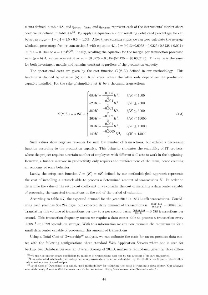
ments defined in table 4.8, and ηcredit, ηdebit and ηprepaid represent each of the instruments’ market share

coefficients defined in table 4.528. By applying equation 4.2 our resulting debit card percentage fee can

be set as rdebit = 1 ∗ 0.4 + 1.5 ∗ 0.6 = 1.3%. After these considerations we can now calculate the average

wholesale percentage fee per transaction b with equation 4.1, b = 0.013∗0.6058+0.0225∗0.3228+0.004∗

0.0714 = 0.0154 or b = 1.54%29. Finally, recalling the equation for the margin per transaction processed

m = (p− b) Ω, we can now set it as m = (0.0275 − 0.0154)52.125 = $0.6307125. This value is the same

for both investment models and remains constant regardless of the production capacity.

The operational costs are given by the cost function G (θ,K) defined in our methodology. This

function is divided by variable (b) and fixed costs, where the latter only depend on the production

capacity installed. For the sake of simplicity let K be a thousand transactions:

G(θ,K) = b θK +

680K +−0.005

2K2, ifK ≤ 1000

520K +−0.004

2K2, ifK ≤ 2500

380K +−0.003

2K2, ifK ≤ 5000

260K +−0.002

2K2, ifK ≤ 10000

180K +−0.001

2K2, ifK ≤ 15000

140K +−0.0005

2K2, ifK > 15000

(4.3)

Such values show negative revenues for such low number of transactions, but exhibit a decreasing

function according to the production capacity. This behavior simulates the scalability of IT projects,

where the project requires a certain number of employees with different skill sets to work in the beginning.

However, a further increase in productivity only requires the reinforcement of the team, hence creating

an economy of scale behavior.

Lastly, the setup cost function I = (K) = aK defined by our methodological approach represents

the cost of installing a network able to process a determined amount of transactions K. In order to

determine the value of the setup cost coefficient a, we consider the cost of installing a data center capable

of processing the expected transactions at the end of the period of valuation.

According to table 4.7, the expected demand for the year 2015 is 18571.146k transactions. Consid-

ering each year has 365.242 days, our expected daily demand of transactions is: 18571146365.242 = 50846.140.

Translating this volume of transactions per day to a per second basis: 50846.14086400 = 0.588 transactions per

second. This transaction frequency means we require a data center able to process a transaction every

0.588−1 or 1.699 seconds on average. With this information we can now estimate the requirements for a

small data center capable of processing this amount of transactions.

Using a Total Cost of Ownership30 analysis, we can estimate the costs for an on-premises data cen-

ter with the following configuration: three standard Web Application Servers where one is used for

backup, two Database Servers, an Overall Storage of 20TB, multi-site redundancy given by three differ-

28We use the market share coefficient by number of transactions and not by the amount of dollars transacted.29Our estimated wholesale percentage fee is approximate to the one calculated by CardFellow for Square. CardFellow

only considers credit card swipes.30Total Cost of Ownership is a widely used methodology for valuating the costs of running a data center. Our analysis

was made using Amazon Web Services metrics for valuation: http://aws.amazon.com/tco-calculator/ .

44

ent telecommunication providers, with a bandwidth of 100Mbps to guarantee a fast connection, and a

”spikey predictable31” usage pattern. However, nowadays there are two ways a company or individual

can provide web applications to their customers: either by running an on-premises data center or by

using a cloud computing service. The following table presents our estimated costs for running an on-site

data center and for using a cloud computing service:

On-premises Amazon WSServers $7630 $2984Storage $85592 $13952Network $72533 $10090Environment $6210 $0Administration $13800 $10350Total/year $185765 $30475

Table 4.9: Estimated costs in USD for a data center and for a cloud computing service.

But cloud computing was not as widespread in 2011 as it is today, so we will use the values for the

on-premises data center. Yet these values are on an annual basis, so we must calculate their present value

for a period of four years. To do so, we must first establish a discount rate for this purpose. Damodaran’s

website32 defines the Weighted Average Cost of Capital for the Information Technology Services sector

as 7.55%. Hence, the cost of the on-premises data center is:

NPV =185.765

1.0755+

185.765

1.07552+

185.765

1.07553+

185.765

1.07554= 621490

This data center valuation points to an average setup cost a of 62149018571.146= 33.465USD per each

thousand transactions.

4.2.3 Volatility

The standard deviation describes the random perturbations around the trend coefficient, whose intensity

is often described in financial literature as volatility (Braumann, 2005). The mobile wallet is a relatively

new product so there is no relevant historical data we can use to estimate its initial volatility. However,

there are other similar products such as the debit card that have been established for years. Considering

there is a relationship between the debit card industry and the proximity mobile payments industry, we

can use real data to estimate the debit card industry volatility. To this end, we used the period from

1990 to 2002:

31Term for large fluctuations on a predictable basis.32Damodaran Online: http://pages.stern.nyu.edu/ adamorar/ .

45

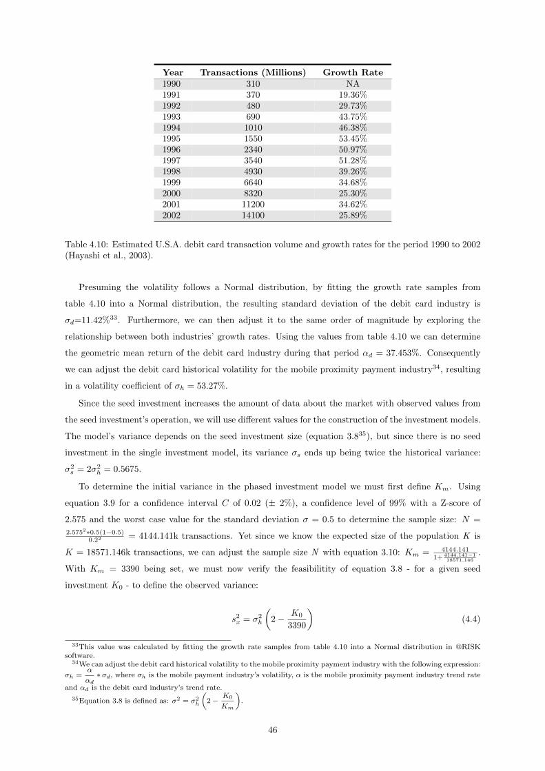
Year Transactions (Millions) Growth Rate1990 310 NA1991 370 19.36%1992 480 29.73%1993 690 43.75%1994 1010 46.38%1995 1550 53.45%1996 2340 50.97%1997 3540 51.28%1998 4930 39.26%1999 6640 34.68%2000 8320 25.30%2001 11200 34.62%2002 14100 25.89%

Table 4.10: Estimated U.S.A. debit card transaction volume and growth rates for the period 1990 to 2002(Hayashi et al., 2003).

Presuming the volatility follows a Normal distribution, by fitting the growth rate samples from

table 4.10 into a Normal distribution, the resulting standard deviation of the debit card industry is

σd=11.42%33. Furthermore, we can then adjust it to the same order of magnitude by exploring the

relationship between both industries’ growth rates. Using the values from table 4.10 we can determine

the geometric mean return of the debit card industry during that period αd = 37.453%. Consequently

we can adjust the debit card historical volatility for the mobile proximity payment industry34, resulting

in a volatility coefficient of σh = 53.27%.

Since the seed investment increases the amount of data about the market with observed values from

the seed investment’s operation, we will use different values for the construction of the investment models.

The model’s variance depends on the seed investment size (equation 3.835), but since there is no seed

investment in the single investment model, its variance σs ends up being twice the historical variance:

σ2s = 2σ2

h = 0.5675.

To determine the initial variance in the phased investment model we must first define Km. Using

equation 3.9 for a confidence interval C of 0.02 (± 2%), a confidence level of 99% with a Z-score of

2.575 and the worst case value for the standard deviation σ = 0.5 to determine the sample size: N =

2.5752∗0.5(1−0.5)0.22 = 4144.141k transactions. Yet since we know the expected size of the population K is

K = 18571.146k transactions, we can adjust the sample size N with equation 3.10: Km = 4144.1411+ 4144.141−1

18571.146

.

With Km = 3390 being set, we must now verify the feasibilitity of equation 3.8 - for a given seed

investment K0 - to define the observed variance:

s2x = σ2h

(2− K0

3390

)(4.4)

33This value was calculated by fitting the growth rate samples from table 4.10 into a Normal distribution in @RISKsoftware.

34We can adjust the debit card historical volatility to the mobile proximity payment industry with the following expression:

σh =α

αd∗ σd, where σh is the mobile payment industry’s volatility, α is the mobile proximity payment industry trend rate

and αd is the debit card industry’s trend rate.

35Equation 3.8 is defined as: σ2 = σ2h

(2 −

K0

Km

).

46

where σ2h is the historical variance and K0 is the seed investment capacity. The test of the average

value on a Normal distribution with unknown variance is done with the t-student test as indicated by

equation 3.43 (Newbold et al., 2007). Assuming the smallest investment’s size aims for a production

capacity of K0 = 150k transactions, or 0.807% of the expected capacity, for a level of significance of 0.1:

1.4695− 1.463250.555√

150

= 0.10474 > t149,0.05 ; θp = 1.4695 ; θp = 1.46325 (4.5)

where θp is the hypothesized mean and θp is the sample mean. The following table provides the results

of the t-test:

t-statistic: 0.10474089Degrees of freedom: 149Critical t-value (two-tailed): +- 1.97601318Two-tailed probability P(h = x): 0.91672226Two-tailed probability P(h 6= x): 0.08327774

Table 4.11: Results of the t-test equation 5.5.

Equation 4.5 validates the idea that a seed investment, even with a reduced production capacity of

K0 = 150k transactions, confirms the feasibility of equation 4.4 for the definition of the model’s variance.

However, since it is a value taken from a sample, the variance coefficient to be used must be tested with

a Chi-Squared distribution36 defined by equation 3.34. For a level of significance of 0.1:

(150− 1) ∗ 0.555

σ20

= 127.419 > χ2149;0,1

where σ20 is the tested variance to be used in the phased valuation model for the given seed investment

K0. Although the resulting σ20 = 0.649 is higher than the initial variance coefficient σ2

s = 0.5675, it will

be subject to the Kalman filter, hence bringing it closer to the real volatility.

4.3 Results of the Investment Models

In this section we present the results obtained from the three investment models: the Single Investment

Model, the Two-Phased Investment Model and the Two-Phased Investment Model with Kalman filter.

Table 4.12 summarizes the main parameters of the models:

36The variance to be tested must be defined according to the size of the sample. That is to say the bigger the sample,the closer the variance gets to the observed value.

47

Parameter Symbol ValueTransaction demand at valuation time D0 326.14kPlanned capacity for transaction processing K 18571.146kMinimum transaction capacity necessary Km 3390kSmallest seed investment transaction processing capacity K0 150kInitial hedged capacity θ0 0.0176Trend rate coefficient α 1.747Historical volatility coefficient σh 0.5327Initial volatility coefficient σs 0.7533Volatility in the smallest seed investment K0 = 150k σp 0.806Expected rate of return ρ 2.05Convenience yield for the single investment δs 0.587Convenience yield for the smallest seed investment K0 = 150k δp 0.628Setup cost in USD a $33.465

Table 4.12: Summary of the models’ parameters.

By analyzing the equation for the parameter β37 of the investment models, we can see that a lower

volatility σ increases the value of β. Furthermore, the optimal hedged capacity equations38 (equations

3.37 and 3.54) show that an increase in the value of β reduces the ratio ββ−1 , hence lowering the value of

the optimal hedged capacity on both models. Moreover, any decrease in the volatility will also decrease

the value of the optimal hedged capacity via the convenience yield coefficient39. As a result, a lower

volatility coefficient leads to a lower optimal hedged capacity, hence resulting in the anticipation of the

investment decision.

To calculate the results for the single investment model, we started by determining the convenience

yield necessary for the investment δs = 0.587 (equation 3.12). Then, we determined the parameter

βs = 1.146 (equation 3.26). Using βS , we calculated the optimal hedged capacity which triggers the

investment decision θ∗s = 0.726 (equation 3.37). Lastly, we determined the expected moment of first

passage with Ingersoll’s (1987) equation: E[T ∗] = 2.543 (equation 3.38).

Convenience yield Optimal hedged capacity Time for investment (years)0.587 0.726 2.543

Table 4.13: Outcome for the single investment model.

The phased investment approach starts by setting a theoretical seed investment production capacity.

Such capacity must be higher than the smallest seed investment transaction processing capacity, since

it must be enough to generate enough information about the market while being less than the current

demand. The initial demand for the project was defined as D0 equal to 326.14k, and the smallest

investment size was defined as K0 equal to 150k transactions. As a result, we considered the following

37Equation for β = 12− ασ2 +

√( ασ2

− 12

)2+ 2ρσ2 .

38The single investment model optimal hedged capacity was defined as θ∗s =βs

βs − 1

δs

m

(2c+ kK

2ρ+ a

)and the optimal

edged capacity for the phased investment model as θ∗p =βp

βp − 1

δp

mK

[K

(2c+ kK

2ρ+ a

)+K0

(2(m− c) − kK0

2ρ+ a

)].

39A lower volatility coefficient will lead to a lower convenience yield coefficient since δ = α− ρ+σ2

2, therefore reducing

the value of the optimal hedged capacity.

48

seed investments’ production capacities in the interval [150k, 326.14k]:

Symbol K0 = 150k K0 = 200k K0 = 250k K0 = 300kObserved variance s2x 0.555 0.551 0.547 0.542Tested variance σ2

p 0.649 0.631 0.617 0.604Volatility σp 0.806 0.794 0.785 0.777Convenience yield δp 0.628 0.618 0.611 0.605Optimal hedged capacity θ∗p 0.788 0.771 0.758 0.748Time for investment in years E[T ∗] 2.668 2.634 2.608 2.585Value of the seed project in USD V0 (1,K0) -8598.713 -11452.756 -14300.701 -17142.549Transaction demand at that time Dt 14634.063k 14318.354k 14076.929k 13891.217k

Table 4.14: Outcome for the phased investment model for each seed investment’s size considered.

For each K0 in table 4.14, we used equation 3.8 to determine the observed variance, followed by

equation 3.43 for the tested variance40. Once the tested variance had been calculated, equation 3.12 was

used to determine the convenience yield coefficient. With the convenience yield being set, we were able

to calculate the βp parameter (equation 3.51). Moreover, after setting these variables we were able to

determine the optimal hedged capacity with equation 3.54. Lastly, we determined the moment of first

passage with Ingersoll’s (1987) equation (equation 3.38).

The seed investments listed in table 4.14 all have a higher volatility coefficient than the one set for

the single investment model, resulting in a higher optimal hedged capacity, therefore in the delay of the

project. This is where the Kalman filter comes in, exploring the use of the information gathered by the

seed investment prototype to reduce the volatility on a weekly basis. To this end we must first find the

weekly equivalents of the variance. For the project’s given annual historical variance σ2h, we can calculate

its weekly equivalent with the following expression σ2h =

(√σ2w√n

)2

(Hull, 1999), with n being the number

of weeks, resulting in a σ2w equal to 0.005457. With that being set, the Kalman filter equation 3.68 only

requires us to define an initial value for the conditional variance St, since the mean value of the sample

µ is equal to α, and on a weekly basis, µ is equal to 0.0196. Epstein et al. (1999) argue we can use any

initial value to St because the Kalman filter corrects itself with the new information it receives41, so we

will use S0 equal to 1. In this approach, the project’s variance is now subject to the Kalman filter through

St and the standard deviation of the samples ξt, with ξt evolving on a weekly basis ξt =

√σw(2− tK0

Km)

n ,

with n being the number of weeks in a year. The following table shows the effect of the Kalman filter -

by applying equation 3.68 - in the variance coefficient on a weekly basis for each of the seed investment

production capacities:

40The tested variances were subject to the Chi-Squared test, and for such investment sizes they all provide a highervolatility coefficient than the one set for the single investment model, although on a decreasing function.

41An inadequate estimate for the first iteration of a Kalman filter will only require more iterations to converge.

49

Variances for each production capacityWeek K0 = 150k K0 = 200k K0 = 250k K0 = 300k

1 0.9086 0.9083 0.9081 0.90792 0.66 0.6558 0.6517 0.64763 0.5765 0.5682 0.5599 0.55164 0.5412 0.5287 0.5162 0.5038...

......

......

11 0.4421 0.4003 0.3586 0.31712 0.4295 0.3836 0.3377 0.297313 0.417 0.3668 0.3168 0.288314 0.4044 0.3501 0.2988 0.285315 0.3919 0.3334 0.2887 0.284316 0.3793 0.3166 0.2854 0.283917 0.3668 0.3002 0.2843 0.283818 0.3542 0.2892 0.284 0.283819 0.3416 0.2856 0.2838 0.283820 0.3291 0.2844 0.2838 0.283821 0.3165 0.284 0.2838 0.283822 0.304 0.2838 0.2838 0.2838...

......

......

26 0.2841 0.2838 0.2838 0.283827 0.2839 0.2838 0.2838 0.283828 0.2838 0.2838 0.2838 0.2838

Table 4.15: Impact of the Kalman filter on the seed investment models’ variance.

Table 4.14 indicates that, for a seed investment of a production capacity of K0 = 150k transactions

it would take 28 weeks to find the real variance coefficient, that is, the historical coefficient σ2h defined

for the project. For K = 200k transactions, the Kalman filter would require 22 weeks instead of 28; for

K = 250k transactions, it would take 19 weeks, while for K = 300k transactions, it would take 17 weeks

to estimate the real volatility. Figure 4.3 shows the effect of the Kalman filter on the variance:

Figure 4.3: Effect of the Kalman filter on the variance through time (weeks).

We can see that the bigger the amount of transactions processed by the seed investment, the faster

we find the real variance coefficient. This effect confirms that the information gathered from a seed

investment depends on its size, although not linearly. We can also study the effect of the Kalman filter

on the evolution of the optimal hedged capacity:

50

Optimal hedged capacitiesWeek K0 = 150k K0 = 200k K0 = 250k K0 = 300k

1 1.0067 1.0049 1.0031 1.00132 0.7961 0.7915 0.7869 0.78243 0.7293 0.7216 0.714 0.70644 0.7016 0.6908 0.6801 0.66955 0.686 0.6721 0.6584 0.64486 0.6744 0.6574 0.6406 0.624...

......

......

11 0.6258 0.5938 0.5624 0.531612 0.6164 0.5815 0.5473 0.517713 0.607 0.5692 0.5323 0.511314 0.5977 0.5571 0.5195 0.509215 0.5884 0.545 0.5124 0.508516 0.5792 0.533 0.5101 0.508217 0.57 0.5213 0.5093 0.508218 0.5609 0.5135 0.509 0.508119 0.5518 0.511 0.509 0.508120 0.5428 0.5101 0.5089 0.508121 0.5338 0.5098 0.5089 0.508122 0.5248 0.5097 0.5089 0.5081...

......

......

27 0.5106 0.5097 0.5089 0.508128 0.5105 0.5097 0.5089 0.5081

Table 4.16: Impact of the Kalman filter on the seed investment models’ optimal hedged capacity.

Table 4.16 shows a decreasing function of the optimal hedged capacity values when the seed investment

size increases, even when they all consider the same variance coefficient. This can be intuitively justified

by the negative cash flows generated by the prototypes (see table 4.14), which affect the optimal stochastic

value and end up anticipating the expansion decision. These cash flows are negative because they all

belong to the same interval of the cost function equation 4.3, which symbolizes that, for a reduced amount

of transactions processed, the operational costs are higher than the margin per transaction processed42.

Next, table 4.17 shows the demand necessary to trigger the expansion decision:

Existing capacity Optimal hedged Demand Additional transactions Timing ofK0 capacity Dt satisfied the investment

150k 0.5105 9480.57 9330.57 2.017 years200k 0.5097 9465.713 9265.713 2.014 years250k 0.5089 9450.856 9200.856 2.012 years300k 0.5081 9435.999 9135.999 2.009 years

Table 4.17: Phased investment models’ demand values that trigger the expansion decision.

Table 4.17 shows a very similar value for the demand needed to trigger the investment decision. Yet,

at the time of the expansion, the additional transactions satisfied by the expansion decision decreases

as the seed investment increases, since the seed investment already installed a transaction processing

capacity. In other words, a smaller seed investment points to a bigger amount of transactions processed

42According to our cash flow equation 3.7, and our cost function 4.3 for a production capacity under K=2500, the revenuefrom a transaction is actually less than the costs it bears.

51

once the expansion happens, provided the delay does not affect the growth of the demand. Moreover,

they all point to an investment happening around the same time, with the difference being partially due

to the effect of the costs they bear (see table 4.14) on the optimal hedged capacity. In short, the smallest

investment ends up providing very similar results than the others while costing less, since they all belong

to the same cost function degree. Also, the best timing for the investment is long after the time the seed

investments take to determine the real variance (28 weeks in the worst scenario), so the investment can

happen at the predetermined date even with the smallest seed investment.

Figure 4.4 represents the cumulative cash flows of the investment project depending on the timing of

the investment43 E[T ]. In it we can see the value rises through time until it reaches a point of inflection,

which represents the maximization of the project, and then starts declining over time:

Figure 4.4: Value of the project depending on the timing of the investment. Time in months. SIM standsfor single investment model and PIM for phased investment model.

The rise prior to the inflection point is justified by the growth rate in the industry, which over time

increases the amount of transactions processed and therefore increases the value of the project. However,

the decline after the inflection point represents the forfeit cash flows for delaying the project too long.

Lastly, the point of inflection from figure 4.4 represents the ideal timing for the investment, since it

maximizes the value of the project.

We can use figure 4.4 for the analysis of the investment models. On one hand, the single investment

model aims for an investment happening in 2.543 years, or 30.516 months, which is six months after the

optimal timing of the ideal investment. Such timing comes after the ideal, representing a loss in cash

flows for delaying the project too much. On the other hand, the phased investment models aim for an

investment happening from 2.017 to 2.009 years, or around 25 months, which is the timing expected for

the ideal investment. This is due to the seed investment’s capacity to generate information about the

market, hence reducing its volatility gradually until it reaches the same value as the real volatility. In

other words, the information gathered by the seed investment ends up anticipating the investment six

months, turning the venture more profitable.

43In our assumptions, following Lint & Pennings (2001), we considered a technology life cycle of four years.

52

Chapter 5

Conclusions

Considering a lack of proper valuation techniques in technology based start-ups, we decided to suggest

a different approach for their valuation. To this end it was necessary to research about the definition of

a NTBF1, the companies’ life-cycles and the valuation models. Due to the limitations of the traditional

models, a Real Options valuation seemed the most suitable. Hence, this paper proposes a two phased

Real Options model, and the use of the Kalman filter to reduce the estimates of the volatility of the

market.

Paydiant belongs to an emerging market characterized by uncertainty. The proximity mobile payment

industry has been growing with the launch of prototypes by Paydiant, Google, Paypal, Square and others.

Different technologies are being incorporated into these wallets and tested, such as Near Field Commu-

nication, visual QR codes2, SMS and USSD3 codes. Market studies predict this type of transactions will

keep rising at huge4 growth rates for the next five years, albeit with a lot of variation between market

studies. Such uncertainty makes this industry attractive for this type of valuation.

Any investment is typically irreversible, but can be delayed until more favorable conditions are present

Dixit & Pindyck (1994). In a phased investment model, the seed investment will provide information

about the market and may allow the manager to take advantage of good outcomes when they become

apparent. The seed investment will serve as a way of retrieving information about the market, hence

reducing the volatility, which in turn will anticipate the time of investment. Furthermore, the Kalman

filter may be applied to the phased investment model to further reduce the volatility, achieving even

better results. Although the economic uncertainty of a project is exogenous to traditional models, under

a Real Options valuation the uncertainty becomes dependent on the size of the seed investment.

When considering an investment of high level investment, we consider two alternatives: a single

investment that covers the whole expected demand, and a phased investment where there is a seed

investment with a follow-on investment. In the second case, the seed investment acts as a source of

information about the market, providing some insight about the moment and size of the expansion

1New Technology Based Firm2Quick Response Code, a two-dimensional bar code which can be read by scanners or cameras in devices.3Unstructured Supplementary Service Data, a protocol used by GSM cellular phones to communicate with the service

provider’s computers.4As an example, eMarketer expects an annual growth rate of about 175% in proximity payments.

53

decision. By using a real options perspective, we can identify the critical value of the hedged capacity

that triggers the expansion decision while considering the volatility associated to it. In a Real Options

perspective, this seed investment is the price of the expansion decision, whose goal is to satisfy the

expected demand.

The phased investment model approach to a technology based start-up, Paydiant, provides a more

adequate valuation when compared to the single investment model. Moreover, the use of Kalman filter

allows for the faster estimation of the volatility, therefore anticipating the definition of the best timing

for the investment. Furthermore, considering the circumstances of Paydiant’s market, the model ends up

anticipating the investment decision. Also, the amount of capital needed to invest in the prototype will

always be smaller than investing in the project as a whole, making the decision about the investment

easier. This study shows the advantages of the seed investment in the financing process of technology

based companies. It achieves this by applying advanced valuation techniques, and then it validates the

theoretical results through the use of Monte Carlo simulation.

54

Bibliography

Agarwal, R., & Audretsch, D. B. (2001). Does entry size matter? The impact of the life cycle and

technology on firm survival. The Journal of Industrial Economics, 49 (1), 21–43.

Alvarez, J., Williamson, E., & Weber, J. (2011). Paydiant. Harvard Business School Marketing Unit

Case(511-065).

Artmann, C., Lechler, T., & Wu, J. (2001). High-growth start-ups-demanding an entrepreneurial growth

theory. In Management of Engineering and Technology, 2001. PICMET’01. Portland International

Conference.

Bar-Ilan, A., & Strange, W. C. (2000). The timing and intensity of investment. Journal of Macroeco-

nomics, 21 (1), 57–77.

Bass, F. M. (2004). Comments on a new product growth for model consumer durables the bass model.

Management science, 50 (12 supplement), 1833–1840.

Bel, J., & Gaza, M. (2012). Innopay: Mobile payments 2012. My mobile, my wallet? Retrieved Novem-

ber 10, 2012 from https://www.innopay.com/publications/mobile-payments-2012-my-mobile-my

-wallet.

Bernanke, B. S. (1983). Irreversibility, uncertainty, and cyclical investment. The Quarterly Journal of

Economics, 98 (1), 85–106.

Bishop, G., & Welch, G. (2001). An introduction to the kalman filter. Proc of SIGGRAPH, Course, 8 ,

27599–3175.

Black, F., & Scholes, M. (1973). The Pricing of Options and Corporate Liabilities. Journal of Political

Economy , 81 , 637-654.

Boyle, P., Broadie, M., & Glasserman, P. (1997). Monte Carlo Methods for Security Pricing. Journal of

Economic Dynamics and Control , 21 (8), 1267-1321.

Braumann, C. (2005). Introducao as Equacoes Diferenciais Estocasticas e aplicacoes. Edicoes SPE,

Lisboa.

Brealey, R., & Myers, S. (2003). Principles of Corporate Finance. McGraw-Hill, Lisbon.

Chabot, C. (1995). Defining High Technology. Techne: Journal of Technology , 5 .

55

Chandra, P. (2008). Financial Management. McGraw Hill, India.

Cox, J., Ross, S., & Rubinstein, M. (1979). Option Pricing: A Simplified Approach. Journal of Financial

Economics, 7 (3), 229-263.

Cukierman, A. (1980). The Effects of Uncertainty on Investment under Risk Neutrality with Endogenous

Information. Journal Political of Economy , 88 (3), 462-475.

Damodaran, A. (2001). The Dark Side of Valuation: Valuing Old Tech, New Tech, and New Economy

Firms. Upper Saddle River, NJ: Prentice Hall, New York.

Day, G. S. (1981). The product life cycle: analysis and applications issues. The Journal of Marketing ,

60–67.

Demers, M. (1991). Investment under uncertainty, irreversibility and the arrival of information over time.

Review of Economic Studies, 58 (2), 333-350.

Dixit, A., & Pindyck, R. (1994). Investment under uncertainty. Princeton, NJ: Princeton Univ. Press.

Dixit, A., & Pindyck, R. (1995). The Options Approach to Capital Investment. Harvard Business

Review , 73 , 105–105.

Dolan, A., & Giffen, B. (1988). The Alberta Junior Capital Pool: Assessing effectiveness as a seed capital

instrument. Journal of Small Business and Entrepeneurship, 6 (1), 19-28.

Epstein, D., Mayor, N., Schonbucher, P., Whaley, E., & Wilmott, P. (1999). The Value of Market

Research When a Firm is Learning: Real Option Pricing and Optimal Filtering. Real Options and

Business Strategy. Applications to Decision Making .

Fontes, M., & Coombs, R. (1997). The coincidence of technology and market objectives in the interna-

tionalisation of new technology-based firms. International Small Business Journal , 15 (4), 14-35.

FRBB. (2012). Consumer Payment Choice: A Central Bank Perspective. Presented to the

2012 Litle Client Conference. http://www.bostonfed.org/economic/cprc/presentations/2012/

Schuh06062012.pdf.

Galbraith, J. K., & Hale, T. (2003, November). Income Distribution and the Information Technology

Bubble. In Presented at the Association of Public Policy Analysis and Management Fall Conference.

http://utip.gov.utexas.edu/papers/utip 27.pdf.

Gassman, O., Escher, J., & Luggen, M. (2003). Spin-off-Grundungen aus privatwirtschaftlichen

Forschungszentren. Wissenschaftsmanagement , 9 (5), 24-30.

Grenadier, S. (1999). Information Revelation through Option Exercise. The Review of Financial Studies,

12 (1), 95-129.

Hayashi, F., Sullivan, R. J., & Weiner, S. E. (2003). A guide to the ATM and debit card industry.

Payments System Research Department, Federal Reserve Bank of Kansas City.

56

Hommel, U., & Knecht, T. (2002). Wertorientiertes Start-up-Management. Munich: Verlag Vahlen.

Hull, J. (1999). Options, Futures, and other Derivatives. Upper Saddle River, NJ: Pearson Education

India.

Ingersoll, J. E. (1987). Theory of financial decision making (Vol. 3). Rowman & Littlefield Pub Incor-

porated.

Jeffery, M. (2004). Return on Investment Analysis for E-business Projects. Internet Encyclopedia(3),

211-236.

Kirkwood, C. (2002). Decision Trees. University Lecture. Arizona State University. Retrieved December

10, 2012 from http://www.public.asu.edu/~kirkwood/DAStuff/decisiontrees/.

Koller, T., Goedhard, M., & Wessels, D. (2005). Valuation: Measuring and Managing Companies. John

Willey & Sons, Inc.

Kotler, P., & Keller, K. L. (2001). Marketing management. Stuttgart, Verlag Schaffer-Poeschel .

Kulatilaka, N., & Perotti, E. (1998). Strategic Growth Options. Management Science, 44 (8), 1021-1031.

Lint, O., & Pennings, E. (2001). An option approach to the new product development process: a case

study at philips electronics. R&D Management , 31 (2), 163–172.

Liptser, R. S., & Shiryayev, A. (2001). Statistics of random processes: I. general theory (Vol. 5). Springer.

Little, A. (1977). New Technology-based Firms in the United Kingdom and the Federal Republic of

Germany. London: Wilton House.

Longoni, A., & Gaza, M. (20123). Innopay: Mobile payments 2013. Changing checkout. Re-

trieved November 10, 2012 from https://www.innopay.com/publications/mobile-payments-2013

-changing-checkout.

Longstaff, F., & Schwartz, E. (2001). Valuing American Options by Simulation: a Simple Least-Squares

Approach. Review of Financial Studies, 14 (1), 79-96.

Lopes, M. F. M. (2007). A decisao de investimento em ambientes de procura incerta [PhD Thesis].

Instituto Superior de Economia e Gestao, Lisboa.

Luehrman, T. (1998). Investment Opportunities as Real Options: Getting Started on the Numbers.

Harvard Business Review , 76 , 51–66.

Luggen, M. (2004). Technology and innovation management in new technology-based firms [MsC Thesis].

Diss., Eidgenossische Technische Hochschule ETH Zurich, Nr. 15400, 2004.

Magee, J. (1964). Decision Trees for Decision Making. Harvard Business Review .

Mbolo, T. U. (2008). Project Valuation using Real Options [PhD Thesis]. Swiss Federal Institute of

Technology Zurich.

57

McDonald, R., & Siegel, D. (1986). The Value of Waiting to Invest. Quarterly Journal of Economics,

101 (4), 707-727.

Moore, G. A. (1991). Crossing the chasm. New York: Harper Business.

Mun, J. (2006). Real options analysis: Tools and techniques for valuing strategic investments and decisions

(Vol. 320). Hoboken, NJ: John Wiley and Sons.

Mun, J. (2010). Modeling Risk: Applying Monte Carlo Simulation, Real Options Analysis, Forecasting,

and Optimization Techniques. Hoboken, NJ: John Wiley and Sons.

Myers, S. (1977). Determinants of Corporate Borrowing. Journal of Financial Economics, 5 , 147-175.

Narayanan, V. (2001). Managing technology and innovation for Competitive Advantage. Englewood

Cliffs, NJ: Prentice Hall.

Neelly, J., & Neufville, R. (2001). Hybrid Real Options Valuation of Risky Product Development Projects.

International Journal of Technology, Policy and Management , 1 (2), 29-46.

Newbold, P., Carlson, W. L., & Thorne, B. (2007). Statistics for business and economics. Pearson

Prentice Hall.

OECD. (1997). Science, Technology and Industry: Scoreboard of Indicators. Organization for Economic

Cooperation and Development, Paris.

Oliveira, A. (2012). Medical Equipment Replacement: Economic Analysis under Deterministic and

Uncertain Environments [MsC Thesis]. Instituto Superior Tecnico, Lisboa.

Quinn, R., & Cameron, K. (1983). Organizational Life Cycles and Shifting Criteria of Effectiveness:

Some Preliminary Evidence. Management Science, 29 (1), 33-51.

Saito, M. B., Junior, J. L. T., & de Oliveira, M. R. G. (2010). A teoria das opcoes reais: uma aplicacao

a projetos de investimento em inovacao tecnologica considerando-se o valor da flexibilidade gerencial.

VII Simposio de Excelencia em Gestao Tecnologia. Pernambuco.

Savioz, P. (2002). Technology Intelligence in Technology-based SMEs. Zurich: Verlag Industrielle Orga-

nization.

Schwartz, E., & Zozaya-Gorostiza, C. (2000). Valuation of Information Technology Investments as Real

Options. Finance Working Paper 6-00.

Triantis, A., & Borison, A. (2001). Real options: state of the practice. Journal of Applied Corporate

Finance, 14 (2), 8–24.

Trigeorgis, L. (1995). Real Options in Capital Investment: Models, Strategies, and Applications. London:

Praeger Publishers.

Wang, Z. (2012). Debit card interchange fee regulation: Some assessments and considerations. Federal

Reserve Bank of Richmond Economic Quarterly , 98 (3), 159–183.

58