1

Communication-Efficient Massive UAV Online Path Control:Federated Learning Meets Mean-Field Game Theory

Hamid Shiri, Jihong Park, and Mehdi Bennis(Invited Paper)

Abstract—This paper investigates the control of a massivepopulation of UAVs such as drones. The straightforward methodof control of UAVs by considering the interactions among them tomake a flock requires a huge inter-UAV communication which isimpossible to implement in real-time applications. One method ofcontrol is to apply the mean field game (MFG) framework whichsubstantially reduces communications among the UAVs. However,to realize this framework, powerful processors are required toobtain the control laws at different UAVs. This requirement limitsthe usage of the MFG framework for real-time applications suchas massive UAV control. Thus, a function approximator based onneural networks (NN) is utilized to approximate the solutions ofHamilton-Jacobi-Bellman (HJB) and Fokker-Planck-Kolmogorov(FPK) equations. Nevertheless, using an approximate solution canviolate the conditions for convergence of the MFG framework.Therefore, the federated learning (FL) approach which can sharethe model parameters of NNs at drones, is proposed with NNbased MFG to satisfy the required conditions. The stabilityanalysis of the NN based MFG approach is presented and theperformance of the proposed FL-MFG is elaborated by thesimulations.

Index Terms—Autonomous UAV, communication-efficient on-line path control, mean-field game, federated learning.

I. INTRODUCTION

Real-time control of a large number of unmanned aerialvehicles (UAVs) is instrumental in enabling mission-criticalapplications, such as covering wide disaster sites in emer-gency cell networks [1], search-and-rescue missions to deliverfirst-aid packets, and firefighting scenarios [2], [3]. One keychallenge is inter-UAV collision, notably under random winddynamics [1], [4]. A straight forward solution is to exchangeinstantaneous UAV locations, incurring huge communicationoverhead, which is thus unfit for real-time operations. Alter-natively, in this article we propose a novel real-time massiveUAV control framework leveraging mean-field game (MFG)theory [5]–[7] and federated learning (FL) [8], [9].

In our proposed FL-MFG control method, each UAV de-termines its optimal control decision (e.g., acceleration) notby exchanging UAV states (e.g., position and velocity), butby locally estimating the entire UAV population’s state dis-tribution, hereafter referred to as MF distribution. Accordingto MFG [6], such a distributed control decision asymptoti-cally achieves the epsilon-Nash equilibrium as the number ofUAVs goes to infinity. To implement this, the UAV needsto solve a pair of coupled stochastic differential equations(SDEs), namely, the Fokker-Plank-Kolmogorov (FPK) and

H. Shiri, J. Park, and M. Bennis are with the Centre for Wireless Com-munications, University of Oulu, 90014 Oulu, Finland (email: hamid.shiri,jihong.park, mehdi.bennis@oulu.fi).

popu

lation FPK HJB

HJBFPK

destinationsource

federated learningwind perturbations

Fig. 1. An illustration of dispatching massive UAVs from a source pointto a destination site. Each UAV communicates with neighboring UAVs forachieving: 1) the fastest travel, while jointly minimizing 2) motion energyand 3) inter-UAV collision, under wind perturbations.

HamiltonJacobiBellman (HJB) equations, for the populationdistribution estimation and optimal control decision, respec-tively. The complexity of solving FPK and HJB increases withthe state dimension, creating another bottleneck in real-timeapplications.

To resolve this complexity issue, FL-MFG control utilizesneural-network (NN) based approximations [4], [10], [11]and FL [8]. Specifically, instead of solving HJB and FPKequations, every UAV runs a pair of two NNs, HJB NN andFPK NN whose outputs approximate the solutions of HJBand FPK equations, respectively. The approximation accuracyincreases with the number of UAV state observations, i.e.,NN training samples. To accelerate the NN training speed,by leveraging FL, each UAV periodically exchanges the HJBNN and FPK NN model parameters with other UAVs, therebyreflecting the locally non-observable training samples. In asource-destination UAV dispatching scenario shown in Fig. 1,simulation results corroborate that FL-MFG control achievesup to 50% shorter travel time, 25% less motion energy, 75%less total transmitted bits, and better collision avoidance mea-sured by 50% lower collision probability number, compared tobaseline schemes: FL-MFG exchanging only either HJB NNor FPK NN model parameters, and a control scheme runningonly HJB NN while exchanging state observations.

A. Background and Related Works

There are many ongoing works on the control and ap-plications of the UAVs. For many missions and tasks suchas agriculture, and search and rescue, the working hours,labor requirements, and cost can be reduced significantly,and the efficiency of the work can also be improved byutilizing the UAVs [12], [13]. However, many current researchworks of UAV such as [14]–[21] are on single UAV withautonomous or manual control, and multiple UAV system

arX

iv:2

003.

0445

1v1

[cs

.NI]

9 M

ar 2

020

2

or mass of UAVs are at the early stages of research [22]–[24]. In [22], an autonomous system is developed to performinspections for precision agriculture based on the use of singleand multiple UAVs. Furthermore, [23] the collective motionof large flocks of autonomous UAVs in order to navigatedin confined spaces is investigated, and it is shown that theswarm behavior remained stable under realistic conditions forlarge flocks and high velocities. In [24] the performance of amultiple UAV system by using the distributed swarm controlalgorithm is evaluated and analyzed through four experimentalcases: single UAV with autonomous control, multiple UAVswith autonomous control, single UAV with remote control,and multiple UAVs with remote control and it is shown thatperformance of the multiple UAV system is better than thesingle UAV system for agricultural application.

Moreover, there are several works considering the flockingbehavior of the agents. In [1] an instantaneous movementcontrol for massive UAVs to provide a cellular connection in adisaster region is investigated. [25] discusses a linear analysisin the synthesis of Cucker-Smale (C-S) type flocking via MFstochastic control theory. It is shown that the C-S flockingbehavior may be obtained as a Nash dynamic competitivegame equilibrium. In [23] a flocking model for real droneswith an evolutionary optimization framework is proposed, andshown that swarm behavior remained stable under realisticconditions for a large population at even high velocities. Theseworks have the common challenge of controlling multipleagents affected randomly by the environment.

MFG framework has been developed mainly in [5]–[7]to study the behavior of large population systems that playnon-cooperative games under exchangeability assumptions.However, the main challenge in this framework is to solve thepartial differential equations (PDEs) with acceptable accuracyand speed for a specific application. There are many numericalmethods to solve PDEs as in [26]–[29]. However, new methodsare arising to obtain the solution for PDE with more accuracyor speed. The (deep) reinforcement learning methods aredeveloped to learn the solution of the HJB equation andcontrol rule in [30]–[32]. In [33] a numerical approximationmethod is proposed to approximate the Kolmogorov PDEwithout suffering from the curse of conditionality. In [10] aneural-network-based online solution of the HJB equation isused to explore the infinite horizon optimal robust guaranteedcost control of uncertain nonlinear systems. However, mostmethods to solve the HJB and FPK are computationallyexpensive, and they are not proper for real-time applications.

Most works in UAV controlling rely on the knowledge ofthe measurements and the environment [34]–[36]. However,obtaining the exact measurements about the environment inrealistic real-time applications is not possible. However, foruncertain or unknown environments the reinforcement learningmodels [14], [37], Bayesian method [38] or models based onMFG [1], [25] can be promising alternatives since they canadapt themselves with the dynamic environment.

To the best of our knowledge, yet there are not many worksconsidering the massive number of UAVs scenario in a windyenvironment in an online manner all together for real-timeapplications. We think that solving this problem can pave the

way for new applications of UAVs.Following [25], in general, two models are used to handle

the massive UAV flocking problem. First, the direct controlmodel where a stochastic differential equation (SDE) at eachUAV should be solved to obtain the control inputs. Second, theMFG theoretic method, where a pair of the partial differentialequation is required to be solved at the UAVs. However, thesetwo models have both advantages and drawbacks for differentapplications.

• In the direct control model, the agents are coupled bya non-linear term in their cost functions. This modelrequires that all the agents have exact information aboutthe states of all other agents in order to solve theircorresponding SDEs. Since this method is base on theexact observations of the other agents, it can result inoptimal solutions. Nevertheless, the application of thismethod is limited to the cases with a small number ofagents because the number of communications increases(exponentially) with the number of agents. Therefore, thedirect SDE method cannot be utilized when the numberof agents is large.

• The mean-field (MF) stochastic control theory can be uti-lized to approximate the large population. In this model,all the agents have similar dynamics and are coupled by anon-linear flocking term in their cost functions. However,this control method requires higher processing at theagents than the direct control method and it should satisfythe convergence conditions. Following [39], MFG theory,as a branch of game theory, is a suitable mathematical toolto help agents of a large population to take proper deci-sions in the context of strategic interactions. When thenumber of agents N in an N -player game increases, thenumber of interactions also increases exponentially andthis makes every exact model for the agents impossibleto be implemented. This problem can be simplified whenthe agents of the system are interchangeable in the sensethat nothing is dependent on an individual agent. Withthis condition, the N -player game can be approximatedby a mean-field, and as a result, the complexity of thegame problem is reduced and it becomes tractable.

Additionally, in the MFG, the optimal control of an agentis obtained by an HJB equation. Then, the FPK equation isused to obtain the joint distribution of the state of agentswhich is used to provide the interactions for the HJB equation.In other words, the MFG framework is a forward/backwardmodel between HJB and FPK equations. However, utilizingthe MFG framework is quite challenging.

• One main challenge for the MFG framework is thatunless for special cases obtaining an analytic solutionfor HJB and FPK differential equations is impossible.Therefore, there is a need for approximate numericalsolutions that require high computations power. There aremany numerical methods such as [27], [28] which canbe used to solve HJB and FPK equations. In addition,deep neural network (DNN) methods are also proposedrecently to solve HJB equations. However, these methodsusually require high processing and might not be suitable

3

for real-time applications with low processing capabilityagents with limited energy.

• Another important challenge in the MFG frameworkis the interchangeability condition for the agents. Thismeans that all the agents play with similar rules. How-ever, if the algorithm used to solve the HJB and FPKequations cannot obtain the optimal solution the agentsmight have different control rules and this will violate theinterchangeability condition.

The proposed method in this paper is to address these chal-lenges.

B. Contributions and Organization

In this paper, we study the real-time control of a largepopulation of UAVs in a windy environment. We start thisby explaining the scenario of multiple UAVs to be movedfrom a starting region to a destination region as shown inFig.1. Next, two control methods are described in detail,i.e. the HJB control method and the MFG control methodto dispatch multiple UAVs quickly, safely, and with lowenergy consumption. Controlling the UAVs by the HJB con-trol method requires that the UAVs know the instantaneouslocation of all the UAVs to achieve the mentioned objective.To reduce the communications cost of HJB, the MFG is auseful alternative. However, obtaining the optimal solution forMFG entails solving a pair of HJB and FPK equation whichis computationally costly, which limits MFG’s usage for real-time UAV control. The main contribution of this paper aresummarized as follows:

• In order to reduce the computational cost of HJB controland MFG control, an NN-based function approximatoris utilized to approximate the solution of HJB and FPKequations in an adaptive way. The method used here isa variant of our previous work in [4], where one single-layer network with two outputs is used to estimate thesolution of each HJB and FPK equations. This methodgives an approximate solution to the HJB and MFGframework.

• In order to validate the feasibility of the proposed method,the Lyapunov stability analysis is used for HJB and FPKapproximation error. These analyses show that the errorof approximate solutions for HJB and FPK is bounded,which means that the obtained approximate control ac-tions from NNs are an approximation of the optimalcontrol actions. However, one main requirement for thestability of the approximate solution of MFG is thatenough data samples should be provided to update NN’sweights, which is challenging in real-time applications.

• To make sure the UAVs do not lack data samples and tomitigate the communication costs, and stability concernsof MFG, an FL-based MFG strategy is proposed, whichwill be named as MfgFL-HF control in this paper. Theperformance and stability of MfgFL-HF are verified bythe simulations. It will be shown that adopting FL canyield faster, safer and energy-efficient control over thebaseline methods.

The remainder of this paper is organized as follows. SectionII describes the system model for controlling the populationof UAVs. Section III explains the HJB and MFG controlmethods and the necessity to propose an alternative method.Section IV proposes the online NN-base method to obtainan approximate solution for HJB and FPK equations, withtheir stability analysis brought in the appendices. Section Vproposes FL-based MFG methods in detail. Section VI vali-dates the performance of the proposed method by simulations,followed by our conclusions in Section VII.

II. SYSTEM MODEL

Consider the scenario of Fig.1, where a set N of N UAVsare set to go from a starting position to a specified destinationin a windy environment. There are three major issues in thisproblem as: A) Dynamics of the control system, whichreflects the relationship between the parameters of the system,and also effect of the environment in the system. The moreinformation we have about the environment, the better modelwe can utilize for control. Here we will assume the windperturbations as the main source of randomness in the system.B) Control problem, which will consider the costs andinterests to formulate a problem where its solution can controlthe UAVs to the destinations. Here, one major assumption forcontrol is that the number of UAVs, i.e. N , is large. Whenthe number of UAVs is getting larger, the complexity and therisk of the problem increases consequently, especially in thereal-time application with expensive UAVs such as UAVs. C)Channel, in a multi-UAV control, the communication amongthe UAVs is of critical importance to achieve the controlobjectives. Here, following the explanations in Introduction,we only will consider inter-UAV channels, which is modeledas Rician in [40]. In the following we will consider thesechallenges to address the objective of the paper. However, themore focus will be on control with more details on the nextsections.

A. Dynamics of Control System

In order to solve the UAV control problem we should obtainthe relationships among its location, speed, acceleration, andeffect of wind on them on the coordinate system. Then Let ususe a Cartesian coordinate system with the origin at the targetposition as the global reference coordinate. We define ri(t) ∈R2 as the vector from the target destination to the currentposition of i-th UAV ui at time t ≥ 0. Therefore, the objectiveof each ui, 1 ≤ i ≤ N , is to gradually reduce the distancebetween destination point and the ui’s current position, bytuning its speed vi(t) ∈ R2 by controlling the accelerationai(t) ∈ R2 under random wind dynamics. Following [41], thewind dynamics are assumed to follow an Ornstein-Uhlenbeckprocess with an average wind velocity vo. The temporal statedynamics are thereby given as:

dvi(t) = ai(t)dt− c0 (vi(t)− vo) dt+ VodWi(t) (1a)

dri(t) = vi(t)dt, (1b)

4

TABLE ILIST OF SIMPLIFIED NOTATIONS.

Notation Simplified MeaningDefinition

ψ(si, t;m(s, t))ψ Value function

ψ(si, t; s−i)φL(si) φL Local termφG(si;m(s, t))

φG Global interaction termφG(si; s−i)f(si) f Drift function∇si ∇ Gradient with respect to∇s∆s ∆ Laplacian with respect to∆s

∇s· ∇· Divergence with respect toH(si, t;m(s, t)) H HJB equationH(si, t; s−i)F(s, t; a(t)) F FPK equationm(s, t) m Distribution of s at time t

wHd(t) wHd

HJB NN modelweights, d ∈ 0, 1

σH(si;m(s, t))σH HJB activation vector function

σH(si; s−i)σF(s) σF FPK activation vector functioneH(si, t) eH Error of approximating HJBeF(s, t) eF Error of approximating FPKJH(wH0

, wH1) JH Loss function of HJB approximation

JF(wF0, wF1

) JF Loss function of FPK approximationai(t) ai Acceleration or control commandεH(si, t) εH Error of HJB with optimal NNεF(s, t) εF Error of FPK with optimal NNLs(si(t)) Ls A Lyapunov candidate functionRi(t) Ri Regularizer term

where c0 is a positive constant, Vo ∈ R2×2 is the covariancematrix of the wind velocity, and Wi(t) ∈ R2 is the stan-dard Wiener process independently and identically distributed(i.i.d.) across UAVs.

Now in order to write the dynamics of the controlled system(1a-1b) in a compact form, let us define the state of each uias si(t) =∆ [ri(t)

ᵀ, vi(t)ᵀ]ᵀ ∈ R4; so the SDEs (1a-1b) can be

rewritten as

dsi(t) = (Asi(t) +B(ai(t) + c0vo)) dt+GdWi(t), (2)

where A =(

0 I0 −c0I

), B = ( 0

I ), G =(

0Vo

), and I denotes

the two-dimensional identity matrix. Furthermore, by definingf(si(t)) = Asi(t) + c0Bvo we rewrite the equation (2), in acompact form as:

dsi(t) = (f(si(t)) +Bai(t)) dt+GdWi(t), (3)

B. Control Problem

In general, a model to solve the mentioned control prob-lem should consider three high-level interests for the UAVs.First, travel time minimization: each UAV i should increasevelocity in the direction to the destination point, to reduce theremaining distance to the destination point while consideringto limit the total velocity of the UAV. Second, motion energy:each UAV i should reduce the (motion) energy consumptionsince the UAVs flight time depends on its battery capacity.Lastly, collision avoidance: the collective interest of thewhole population is to make a flock of the UAVs travelingtogether to avoid UAVs colliding each other and also to

complete the mission quickly. Nevertheless, there is a trade-offamong the interests which should be considered in the controlproblem.

To achieve the aforementioned interests, UAV ui at timet<T aims to minimize its average cost ψaii (si, t; s−i), wheresi(t) = si, s−i(t) = s−i are the state of UAV ui and the setof states of all UAVs excluding UAV ui at time t, respectively,and the average is taken with respect to the measure inducedby control law ai for τ ∈ [t, T ]. The cost ψaii (si, t; s−i)consists of the term g(ai(τ), si(τ); s−i(τ)) depending only onthe local state si(τ) and the control action ai(τ) with givenstates of other UAV’s as s−i(τ).

ψai(si, t; s−i)=E[ ∫ ᵀ

t

g(ai(τ), si(τ); s−i(τ))dτ]

(4)

where E is the expectation operator, andg(ai(τ), si(τ); s−i(τ)) is

g(ai(τ), si(τ); s−i(τ))=φL(si(τ))+ c3‖ai(τ)‖2

+c2φG(si(τ); s−i(τ)) (5)

in which, the term φL(si(τ)) depending only on the local statesi(t) and the term φG(si(τ); s−i(τ)) relying on the globalstate si(t), s−i(t), are given as:

φL(si(τ)) =vi(τ) · ri(τ)

‖ri(τ)‖ + c1‖vi(τ)‖2, (6)

φG(si(τ); s−i(τ)) =1

N

∑uj∈N

‖vj(τ)− vi(τ)‖2(ε+ ‖rj(τ)− ri(τ)‖2

)β , (7)

and the terms c1, c2, c3, β, and ε are positive constants.The local term φL(si(τ)) and the second term in (5)

focus on the the two objectives, i.e. travel time and mo-tion energy minimization. It is intended to minimize theremaining travel distance ‖ri(τ)‖ by maximizing the velocitytowards the destination, i.e., minimizing the projected velocityvi(τ) · ri(τ)/‖ri(τ)‖ towards the opposite direction to thedestination. Also, it is planned to minimize the kinetic energyand the acceleration control energy that are proportional to‖vi(τ)‖2 and ‖ai(τ)‖2, respectively [21], [25]. Then, themotion energy E(t) for each UAV i at time t, is defined as

E(t) =

∫ t

τ=0

(c2‖vi(τ)‖+ c3‖ai(τ)‖)dτ, (8)

which is used as a metric to compare different algorithms inthis paper.

The global term φG(si(τ); s−i(τ)) in (5) refers to colli-sion avoidance, and is intended to form a flock of UAVsmoving together [42]. The flocking leads to small relativeinter-UAV velocities for avoiding collision even when theircontrolled velocities are slightly perturbed by wind dynamics.A collision happens when the inter-UAV distance is lessthan a defined distance rcoll. Furthermore, the flocking yieldscloser inter-UAV distances without collision. This is beneficialfor allowing more UAVs to exchange their states throughbetter channel quality, thereby contributing also to collisionavoidance. The formation of a flock as mentioned in [43] isa result of three components: a) separation, i.e. steer to avoidcrowding; b) alignment, i.e. steer toward the average headingof neighbors; c) cohesion, i.e. steer toward the average positionof neighbors. In view of this, we adopt the Cucker-Smale

5

flocking [1], [42] that reduces the relative velocities for theUAVs. The relative velocity ‖vj(τ) − vi(τ)‖ and the inter-UAV distance ‖rj(τ) − ri(τ)‖ are thus incorporated in thenumerator and denominator of φG(si(τ); s−i(τ)), respectively.In addition, inspired by [23], the velocity alignment φA(t) andnumber of collision risks φC(t) as metrics to compare differentalgorithms, are defined as

φA(t) =1

tN2

∫ t

0

∑ui∈N

∑uj∈N

‖vj(τ)− vi(τ)‖dτ , (9)

φC(t) =1

tN2

∫ t

0

∑ui∈N

∑uj∈N

1‖rj(τ)−ri(τ)‖≤rC dτ , (10)

where the hazard radius rC defines a dangerous potentialcollision zone around the UAV. Lower values of φA(t) meansthat the amplitude of velocity difference between UAVs issmall and hence they have made a better flock to traveltogether. Lower values of φC(t) mean that the UAVs do nottend to be too close to each other and the risk of them collidingeach other is smaller.

Incorporating the cost (4) under the temporal dynamics (3),the control problem of UAV ui at time t is formulated as:

ψ(si, t; s−i) = minai

ψai(si, t; s−i) (11)

s.t. dsi(t) = (f(si(t)) +Bai(t)) dt+GdWi(t), (12)

The minimum cost ψ(si, t; s−i) is referred to as the valuefunction of the optimal control, and should be derived to obtainthe optimal action ai(t) for UAV ui. The methods to encounterthis problem will be introduced in the following sections.

C. UAV to UAV Wireless Channel Model

In many multi-UAV control problems, communicationamong the UAVs is a critical condition. However, in the prob-lem of this paper the UAVs will be required to communicatetheir data with each other while they are moving at a height h.Following [44] for the UAV to UAV communication channels,the Rice model can be used to model both dominant LOS andNLOS paths. The rice distribution is given by:

pz(ζ) =ζ

χ2exp

(−ζ2 − ξ2

2χ2

)I0

(zξ

χ2

), (13)

where ζ ≥ 0, and ξ and χ are the strength of LOS and NLOSpaths respectively. Assuming the frequency division multipleaccess (FDMA) is used for each UAV to UAV communication,with the transmission power Po, and the distance rd from aUAV to another UAV, the received signal-to-noise (SNR) ateach time is:

SNR =Pozr

−αd

Woσn, (14)

where, σn is the noise power, Wo is the bandwidth, α ≥ 2 isthe path loss exponent, and z is the rice random variable de-fined in (13) and is assumed to be independent and identicallydistributed (i.i.d) across the different UAVs and times.

Another parameter which we will use in this paper is thecommunication latency. A signal is successfully decoded if theSNR at time t is greater than a target SNR η, i.e., SNR(t) ≥ η.The number of bits bi(D0), transmitted during D0 time slots,is given as:

bi(D0) = θ

D0∑t=1

1SNR(t)≥ηWo log2(1 + η), (15)

where θ is the channel coherence time. The latency of trans-mitting b bits is the minimum D0, i.e. Dm that satisfiesbi(D0) ≥ b. A latency outage occurs when Dm is greater thana predefined threshold DM , i.e., Dm > DM in an algorithm.

III. HJB AND MFG CONTROL

At each time instant, each UAV seeks a solution for thedefined objective function. The first intuitive method is toanalyze the problem directly as solving an HJB equation andthen see if there is a need for other alternatives and also havethe basis for the proposed methods. However, in the following,it will be clarified that when the number of UAVs is high,the communications and processing complexity will increaseto the extent that the real-time implementation will not bepossible. Therefore, an alternative MFG method which canreduce the number of communications significantly will beexplained.

A. HJB Control

In this method, we assume that all UAVs perform theiroptimal action based on the last observed states of all otherUAVs and not their instantaneous action and states. Therefore,the HJB equation with this method is obtained as

ψ(si, t; s−i) + minaig(ai(t), si; s−i)

+ [∇siψ(si, t; s−i)]ᵀ (f(si) +Bai(t))

+1

2tr(GGᵀ[∆siψ(si, t; s−i)]) = 0, (16)

where ∇ and ∆ denote the gradient and Laplacian operators,respectively. The optimal action at UAV i is obtained as

ai(t) = − 1

2c3Bᵀ∇siψ(si, t; s−i). (17)

Therefore, substituting (17) in (16) yields in HJB equation

ψ(si, t; s−i) + φL(si)+c2φG(si; s−i)

+

(f(si)−

1

4c3BBᵀ∇siψ(si, t; s−i)

)ᵀ

[∇siψ(si, t; s−i)]

+1

2tr(GGᵀ[∆siψ(si, t; s−i)]) = 0. (18)

Solving this HJB equation requires an enormous exchange ofstates among the UAVs, which becomes impossible when thenumber of UAVs, i.e. N , is high. In order to address thischallenge, we leverage the capabilities of the MFG frameworkexplained in the next subsection. Therefore, the UAVs onlywill need to exchange the states only at the beginning of themission, and after that, they will calculate the optimal actionsbased on their own state.

6

B. MFG ControlAnother method to encounter this problem is to use MFG

framework when the number of UAVs is very high. LetmN (s, t) be the empirical state distribution function of theUAVs at time instant t defined as

mN (s, t) =∆1

N

N∑j=1

δ(s− sj(t)), (19)

where δ(·) is the Dirac delta function. Then, the interactionterm (7) can be rewritten as

φG(si(t); s−i(t)) =

∫s

mN (s, t)‖vi(t)− v‖2

(ε+ ‖ri(t)− r‖)2)βds. (20)

Since the states si(t) for i = 1, . . . , N are independent andidentically distributed which evolve according to SDE (12),utilizing the ergodic theory gives

limN→∞

mN (s, t) = m(s, t), (21)

where m(s, t) is the distribution of generic UAV’s state, i.e., s,according to the SDE (12) and the optimal policy a(t) obtainedby (17). The distribution m(s, t), which is called mean field(MF), is a solution of the Fokker-Plank-Kolmogorov (FPK)equation which is derived from the SDE (12) as

m(s, t) +∇s · [(f(s) +Ba(t))m(s, t)]

− 1

2tr(GGᵀ∆sm(s, t)) = 0, (22)

where ∇s· denotes the divergence operator, and the initialdistribution of the UAVs is given as m(s, 0) = 1

N

∑Nj=1 δ(s−

sj(0)). Hence, the solution to equation (22), i.e., m(s, t), canbe used to obtain the interaction term as

φG(si(t);m(s, t)) =∆∫s

m(s, t)‖vi(t)− v‖2

(ε+ ‖ri(t)− r‖)2)βds (23)

By this definition, the HJB equation (18) can be rewritten asψ(si, t;m(s, t)) + φL(si)+c2φG(si;m(s, t))

+

(f(si)−

1

4c3BBᵀ∇siψ(si, t;m(s, t))

)ᵀ

[∇siψ(si, t;m(s, t))]

+1

2tr(GGᵀ[∆siψ(si, t;m(s, t))]) = 0, (24)

and the corresponding action is

ai(t) = − 1

2c3Bᵀ∇siψ(si, t;m(s, t)), (25)

Therefore, by substituting (25) in (22) the FPK equation canalso be rewritten in the following form:

m(s, t) +∇s · [(f(s)− 1

2c3BBᵀ∇sψ(s, t;m(s, t)))m(s, t)]

− 1

2tr(GGᵀ∆sm(s, t)) = 0 (26)

By solving HJB and FPK equation pairs, i.e., (24) and (26),the optimal action for each UAV can be calculated.

IV. NN-BASED HJB AND MFG LEARNING CONTROL -STATE SHARING METHODS

In this section, inspired by [45], we discuss NN-basedmethods to obtain approximate solutions for HJB and FPKequations for the multiple UAV control application. However,to have better readability and also to save space, we use thesimplifications of Table I, and whenever required we will usethe complete forms to avoid confusion.

A. HJB Learning Control

Here, following our previous work [REF], we find anapproximate solution to the HJB equation to obtain the cor-responding action. Any approximate solution will result insome error, and the approximated HJB equation may not beexactly equal to zero. However, first, based on the definedsimplifications above, we represent the HJB equation (18) and(24) by H as

H =∆ ψ +

(f − 1

4c3BBᵀ∇ψ

)ᵀ

∇ψ

+ φL+c2φG+1

2tr(GGᵀ∆ψ) = 0, (27)

where we obtain the φG empirically by (7) in this subsection.Similar to [45], given the state distribution of UAVs at

each time t, let the function ψ(si, t; s−i) and its derivativecorrespondingly be approximated by functions as

ψ(si, t; s−i) =∆ wH0(t)ᵀσH(si; s−i) , (28)

ˆψ(si, t; s−i) =∆ wH1(t)

ᵀσH(si; s−i) , (29)

where vector functions wH0(t) and wH1

(t) are approximationsto the optimal vector weight functions wH0

(t) and wH1(t),

respectively, and the value error of these approximations are

εH0(si, t) =∆ ψ(si, t; s−i)− wH0(t)ᵀσH(si; s−i) , (30)

εH1(si, t) =∆ ψ(si, t; s−i)− wH1(t)ᵀσH(si; s−i) . (31)

Then, using these definitions, and notation simplifications asin Table I, the HJB equation (27) and its approximatation arewritten as

H = wᵀH1σH +

(f − 1

4c3BBᵀ([∇σH]ᵀwH0)

)ᵀ

[∇σH]ᵀwH0

+1

2

[N∑k=1

tr(GGT [∆σ[k]H ])ek

]ᵀwH0 +φL+c2φG+εH =0,

(32)

H = wᵀH1σH +

(f − 1

4c3BBᵀ([∇σH]ᵀwH0)

)ᵀ

[∇σH]ᵀwH0

+1

2

[N∑k=1

tr(GGT [∆σ[k]H ])ek

]ᵀwH0 + φL+c2φG, (33)

where the superscript [k] shows the k’s element of the corre-sponding vector, ek is a vector with k’s element equal to 1and other elements equal to zero, and εH is the error of HJBequation with the function approximator defined as

εH =c2εφG + εH1

− 1

4c3[∇εH0 ]ᵀBBᵀ[∇σH]ᵀwH0 −

1

4c3[∇εH0 ]ᵀBBᵀ∇εH0

+

(f − 1

4c3BBᵀ[∇σH]ᵀwH0

)ᵀ

∇εH0 +1

2tr(GGᵀ∆εH0)

(34)

where εφGis the uncertainty of the interaction term. Then, the

corresponding approximate action can be obtained by

a = − 1

2c3Bᵀ[∇σH]ᵀwH0 −

1

2c3Bᵀ[∇εH0 ], (35)

a = − 1

2c3Bᵀ[∇σH]ᵀwH0 . (36)

Therefore, the error of approximating HJB equation by NNsis

7

Algorithm 1 Hjb control1: Initialization: wH0(n) = 0 and wH1(n) = 0.2: for Each UAV i = 1, . . . , N , in parallel, do3: Collect the states s−i(t) from neighboring UAVs.4: Update the weights wH0

(n) and wH1(n) by (39) and

(40).5: Calculate the value ψ = wᵀ

H0σH.

6: Take the optimal action a=− 12c3Bᵀ[∇σH]ᵀwH0

.7: end for

eH =H− H

=− wᵀH1σH − w

ᵀH0

[∇σH]f −1

4c3wᵀ

H0[∇σH]BBᵀ[∇σH]ᵀwH0

+1

2c3wᵀ

H0[∇σH]BBᵀ[∇σH]ᵀwH0

−1

2

[N∑k=1

tr(GGT [∆σ[k]H ])ek

]ᵀ

wH0− εH, (37)

where wH0 =wH0−wH0 , and wH1 =wH1−wH1 . Then, the optimalweights wH1and wH0should minimize the loss function definedas

JH(wH0 , wH1)=1

2eᵀHeH+cH max

0, Ls

1‖si(t)‖≥sdest︸ ︷︷ ︸

Ri

(38)

where cH is a positive constant, Ls as the simplified notationof Ls(si(t)) is a Lyapunov candidate function, and Ls is itsderivative with respect to time. The regularizer term shown asas Ri or Ri(t) is meant to stop the movement when reachingthe destination, i.e., si(T ) = [ri(T )ᵀ, vi(T )ᵀ]ᵀ ≤ sdest. Then,by discretizating the time with dt steps, the gradient descentupdates are written as

wH0(n+1)= wH0(n)−µH(∇wH0eH)eH−µHcH∇wH0

Ri, (39)

wH1(n+1)= wH1(n)−µH(∇wH1eH)eH, (40)

where the gradients ∇wH0eH and ∇wH1

eH are obtained as∇wH0

eH =[∇σH]f +1

2

[N∑

k=1

tr(GGT [∆σ[k]

H ])ek

]

+1

2c3[∇σH]BBᵀ[∇σH]ᵀwH0

−1

2c3[∇σH]BBᵀ[∇σH]ᵀwH0

,

(41)∇wH1

eH =σH. (42)

The corresponding Hjb learning control based on these up-date equations is described in Algorithm 1. After initializationof the weights, each UAV has to collect instantaneous states ofother UAVs and use it to update the equations (39) and (40).Then, it uses the updated model to take the proper action.However, the stability of this algorithm is explored by thefollowing Proposition 1.Proposition 1 (HJB Lyapunov stability): For small uncer-tainty of interaction term, i.e., ‖εφG‖ 1, and a boundedinteraction term, i.e., ‖φG‖ ≤ M1, the system state and themodel weights of constructed adaptive HJB neural networkobtained by Algorithm 1 are uniformly ultimately bounded(UUB).

The UUB means that there exist sdest, w0, and w1 at timeT such that ‖s(t)‖≤sdest, ‖wH0(t)− wH0(t)‖≤w0, and ‖wH1(t)−wH1(t)‖≤w1 for all t ≥ T + T ′.

Proof. See Appendix A.

B. MFG Learning Control

Here, we find an approximate solution to the pair of HJB-FPK equations in MFG framework. Regarding the HJB equa-tion, we follow the method explained in previous subsectionand by considering that the interaction term is obtained using(23). Then, we follow the similar approximation procedure toapproximate the solution for FPK equation. Let us first rewritethe FPK equation (26) by using the simplified notations inTable I, and define F as

F = m+∇ · [(f − 1

2c3BBᵀ∇ψ)m]− 1

2tr(GGᵀ∆m) = 0 (43)

Using the equality ∇ · [a~b] = a∇ ·~b+~bᵀ∇a, where ~b is avector and a is scalar, we rewrite this FPK equation as

F = m+m∇ · [(f − 1

2c3BBᵀ∇ψ)]

+ [(f − 1

2c3BBᵀ∇ψ)]ᵀ∇m− 1

2tr(GGᵀ∆m) = 0 (44)

Now, we seek to find an approximate solution to the equation(44). Let us define the linear function approximator m(s, t),which approximates the density function m∗(s, t), as

m(s, t) =∆ wF0(t)ᵀσF(s) , (45)ˆm(s, t) =∆ wF1(t)ᵀσF(s) , (46)

where σF(s) is a vector of linear or nonlinear functions,and wF0

(t) and wF1(t) are the approximation to the optimal

weight functions wF0(t) and wF1

(t) respectively. Then, theerrors of approximating the distribution function m(s, t) andits derivative m(s, t) are

εF0(s, t) = m(s, t)− wF0(t)ᵀσF(s) , (47)εF1(s, t) = m(s, t)− wF1(t)ᵀσF(s) . (48)

Considering this definition, and notation simplifications ofTable I, the FPK equation (43) and its corresponding approx-imatation are written as

F = wᵀF1σF + wᵀ

F0σF∇ · [(f −

1

2c3BBᵀ∇ψ)]

+ [(f − 1

2c3BBᵀ∇ψ)]ᵀ[∇σF]ᵀwF0

− 1

2

[N∑k=1

tr(GGT [∆σ[k]F ])ek

]ᵀwF0 + εF = 0, (49)

F = wᵀF1σF + wᵀ

F0σF∇ · [(f −

1

2c3BBᵀ∇ψ)]

+ [(f − 1

2c3BBᵀ∇ψ)]ᵀ[∇σF]ᵀwF0

− 1

2

[N∑k=1

tr(GGT [∆σ[k]F ])ek

]ᵀwF0 , (50)

where εF denotes the error of FPK equation caused by theNN, and it is defined as

εF =∆ ∇ · [(f − 1

2c3BBᵀ∇εψ)(wᵀ

F0σF + εF0)]

+ εF1 + εF0∇ · [(f −1

2c3BBᵀ∇ψ)]

+ [(f − 1

2c3BBᵀ∇ψ)]ᵀ[∇εF0 ]

− 1

2tr(GGᵀ∆εF0), (51)

where εψ is the uncertainty in finding ψ. Therefore, the errorof approximating FPK equation by neural networks is

8

Algorithm 2 Mfg control1: Initialization: m(s, 0) = 1

N

∑Nj=1 δ(s−sj(0)), wH0(n) = 0,

wH1(n) = 0, wF0(n) = 0, wF1(n) = 0 .2: for Each UAV i = 1, . . . , N , in parallel, do3: for n = 1, . . . , T0 do4: Update weights wH0

(n) and wH1(n) by (39) and (40).

5: Calculate value ψ = wᵀH0σH.

6: Update weight wF0(n) and wF1

(n) by (54) and (55).7: Obtain MF distribution m = wᵀ

F0σF.

8: end for9: Take the optimal action a=− 1

2c3Bᵀ[∇σH]ᵀwH0 .

10: end for

eF =F− F=− wᵀ

F1σF

− wᵀF0σF∇ · [(f −

1

2c3BBᵀ∇ψ)]

− wᵀF0

[∇σF][(f − 1

2c3BBᵀ∇ψ)]

+1

2wᵀ

F0

[N∑k=1

tr(GGT [∆σ[k]F ])ek

]− εF, (52)

where wF0 = wF0−wF0 , and wF1 = wF1−wF1 . Based on thesedefinitions, the optimal weights wF1and wF0 should minimizethe loss function defined as

JF(wF0 , wF1) =1

2eᵀFeF (53)

Therefore, by discretizating the time with dt time steps, andthe gradient descent updates for FPK weights are obtained as

wF0(n+1)= wF0(n)−µF(∇wF0eF)eF (54)

wF1(n+1)= wF1(n)−µF(∇wF1eH)eF (55)

where the gradients ∇wF0eF and ∇wF1

eF are

∇wF0eF = σF∇ · [(f−

1

2c3BBᵀ∇ψ)] + [∇σF][(f− 1

2c3BBᵀ∇ψ)]

− 1

2

[N∑k=1

tr(GGT [∆σ[k]F ])ek

](56)

∇wF1eF = σF. (57)

However, based on these update pairs and update pairs forHJB equation, the Mfg learning algorithm is described as inAlgorithm 2. In this algorithm, first, the UAVs share theirstates sj(0) at time t = 0 to obtain the distribution of thepopulation and initial samples. Then, the UAVs start collectingsamples and and updating theirs weights untill they reach thedestination at time T = T0dt.

We have shown in our previous works [4] that this methodprovides better results in terms of energy consumption, com-munications cost, and flocking of UAVs when enough samplesare used to train the models. However, there is stabilityconcerns about this algorithm which is guaranteed in thefollowings.Proposition 2 (FPK Lyapunov stability): For almost certainψ, i.e., ‖εψ‖1, and differentiable and bounded value functionψ, i.e., ‖ψ‖ ≤ M2, the weights of constructed adaptive FPK

neural network obtained in Algorithm 2, which is controlledby its corresponding HJB equation, are UUB.

The UUB means that there exist w2, and w3 at time T suchthat ‖wF0(t) − wF0(t)‖≤w2, and ‖wF1(t) − wF1(t)‖≤w3 for allt ≥ T + T ′.

Proof. See Appendix B.

Proposition 3 (FPK Convergence): Under the assumptionsof Proposition 2 and with small step-sizes µF, the weights ofFPK neural network function approximator converges to itsoptimal weights in mean with no bias and it is stable in meansquare deviation sense.

Proof. See Appendix C.

Corollary 1: Considering Propositions 1, 2, and 3, we canconclude that the system state and weights of constructed HJB-FPK neural networks obtained by Algorithm 2 are UUB.

Proof. The Algorithm 2 has two parts as HJB part and FPKparts. It is initialized by the states of the UAVs at the sourceregion. At the initial iterations the states are used directly inthe algorithm to update the weights of HJB and FPK neuralnetworks, and hence the uncertainty of interaction term issmall, i.e., ‖εφG‖ 1. Also, by starting with well trained orzero initialized neural network weights, both the interactionterm and value functions are upper-bounded, i.e., ‖φG‖ ≤M1

and ‖ψ‖ ≤ M2. Hence, there is a design, i.e., a choice ofparameters in proofs in Appendices A, B, and C, such thatall assumptions necessary for Propositions 1, 2, and 3 holdtogether and completely

V. FEDERATED MFG LEARNING - MODEL SHARINGMETHODS

In this section, we propose federated mean field gamelearning strategy (MfgFL) and its different implementations,i.e., MfgFL-H, MfgFL-F, and MfgFL-HF, to make the UAVs’control models close to each other and to use sample diversityamong the UAVs efficiently. In MfgFL-H the model param-eters of HJB neural network are shared with central unit toobtain the global HJB NN model, so the action rules of UAVsare close to each other. In MfgFL-F the FPK NN models aretransmitted to the central unit to obtain the global FPK NNmodel, so the estimation of the population density function atUAVs be more accurate. In MfgFL-HF, both HJB and FPKneural network models are averaged to obtain better globalonline MFG learning model. In the following, we explaingeneral form of MfgFL strategy, which covers three differentimplementations.

Although Algorithm 2 can reduce the communications costof the control algorithm by leveraging the MFG framework, itstill requires big sample sets to train and provide conditions ofstability. In other words, there is still a need to share a subset ofsamples among the UAVs or with a central unit, which requiresextra communication costs in addition to privacy concerns.Therefore, instead of state sharing, we adopt the federatedlearning method to address these issues.

In the MfgFL algorithm, one UAV out of all is set to actas a control center, which we call is as leader (or header)

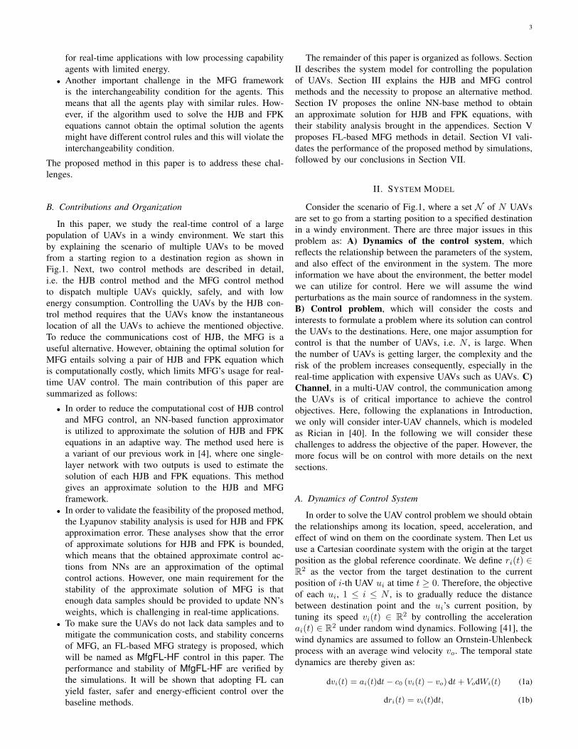
9

Algorithm 3 MfgFL control1: Initialization: m(s, 0) = 1

N

∑Nj=1 δ(s−sj(0)), wH0(n) = 0,

wH1(n) = 0, wF0(n) = 0, wF1(n) = 0 .2: for n = 0, 1, 2, . . . , T0 do3: if n = kn0 then4: Nh UAVs, in parallel, send their model wi,d(kn0) to

the leader.5: leader updates the model parameters wh,d(k), via

wh,d(k)← 1

Nh

∑i∈Nh

wi,d(kn0), (58)

6: leader broadcasts the model wh,d(k).7: end if8: for each UAV i = 1, . . . , N , in parallel, do9: if UAV i receives wh,d(k) then

10: Update wi,d(n) as

wi(n)← wh,d(k) (59)

11: end if12: Update wH0

(n), wH1(n), wF0

(n), and wF1(n) by (39)

and (40), (54), and (55).Take the optimal action a=− 1

2c3Bᵀ[∇σH]ᵀwH0 .

13: end for14: end for

UAV. This leader UAV depending on the application may bechosen randomly or considering UAVs power consumption orflight time, which is beyond the scope of this work. Then, wesimply set one of the UAVs as the leader, i.e., uh, and indicateit by index h in the algorithm.

The proposed MfgFL learning control is described inAlgorithm 3. Following the FedAvg algorithm, the leadercollects models wi,d(n) of Nh UAVs at times n = kn0,where d ∈ H,F,HF with corresponds to three types ofimplementation as

• In MfgFL-H, i.e., d = H, the model wi,d(n) is equalto the set wH0(n), wH1(n) of the corresponding UAVi. However, the FPK models wF0(n), and wF1(n) are notshared in this implementation.

• In MfgFL-F, i.e., d = F , the model wi,d(n) is equalto the set wF0(n), wF1(n) of the corresponding UAVi. However, the HJB models wH0(n), and wH1(n) are notshared in this implementation.

• In MfgFL-HF, i.e., d=HF , the model wi,d(n) is equalto the set wF0(n), wF1(n), wH0(n), wH1(n) of the corre-sponding UAV i. In other words, the complete model ofMFG is shared with the leader.

The leader obtains the average model wh,d by (58) aftercollecting models from other UAVs. However, after the aver-age model is calculated at the leader and broadcasted to theUAVs, the updates are done locally by local samples at eachUAV. Then, this procedure is repeated until all the UAVs reachthe destination at repetition T0.

In addition to reducing communication costs and increasingthe privacy of the UAVs, the MfgFL method can provideother benefits as well such ensuring stability conditions for

MFG framework and increasing training speed. One majorcondition for the MFG based approach is that the UAVs are in-distinguishable. It means that the UAVs should have the sameaction rule, and hence, it is reasonable that they are trained bybig enough samples. Nonetheless, due to energy/bandwidthlimitations, it is not possible to provide this huge samplesfor model training. From this viewpoint, FL-based approachescan increase the model similarity among the UAVs and makethem indistinguishable by efficiently using their samples fortraining.

Another benefit of using the MfgFL approach is the in-creased training speed of the models at UAVs. This is closelyrelated to the communication cost of the algorithm, since uti-lizing model averaging means that the algorithm benefit fromthe various sample of UAVs in a shorter time span. Therefore,it is safe to say that it can provide higher model trainingspeed. However, the performance of MfgFL is explored innext section.

VI. NUMERICAL RESULTS

In this section, we numerically validate the effectiveness ofthe proposed algorithm MfgFL-HF compared to the baselinemethods Hjb control, MfgFL-F, and MfgFL-H, in terms oftravel time, motion energy, collision avoidance, and communi-cations cost. Throughout the simulations, we consider N UAVscontrolled in a two-dimensional plane at the fixed altitude ofh = 40m. Initially, the UAVs are equally separated with thedistance

√2m each other, and located at a source, which is

a square region centered at (150, 100)m in a 2-dimensionalplane (see Fig. 2-a). Each UAV aims to reach the destinationat the origin, under the wind dynamics described by Vo = 0.1I

and vo = (1,−1)m/s (see Sec. II).Following [4], [10] single hidden layer models (28) and

(29) are considered for HJB model, where each hidden node’sactivation function, i.e., σH,j(si(t)) for j = 1, · · · ,MH, cor-responds to each scalar term in a polynomial expansion. Thepolynomial for σH(si(t)) is heuristically chosen as: (1+xi(t)+

vx,i(t))6 +(1+yi(t)+vy,i(t))

6, where ri(t) = [xi(t), yi(t)]ᵀ and

vi(t) = [vx,i(t), vy,i(t)]ᵀ, thus the model size for HJB model is

MH =54.For the MFG based methods, the same neural network

structure described above is considered to approximate HJBmodel. In a similar way, single hidden layer models (47)and (48) are considered for FPK model, where each hiddennode’s activation function, i.e., σF,j(si(t)) for j = 1, · · · ,MF,corresponds to each scalar term in a polynomial expansion.The polynomial for σF(si(t)) is heuristically chosen as: (1 +

xi(t) +vx,i(t))6 + (1 +yi(t) +vy,i(t))

6. Thus the model size forFPK model is MF =69.

Unless otherwise stated, the default simulation parametersare: Po = 20dBm, Wo = 2MHz, σn = −110 dBm/Hz, α = 0,χ = 1.347, ξ = 6.649; n0 = 100, Nh = 0.8N ; rcoll = 0.1m, rC =√

2/2m; c0 = 0.1, c1 = c2 = 0.015, c3 = 0.005, µH = µF = 0.01,cH = 0.5 and dt = 0.1s for the purpose of discretizing time insimulations.

Fig. 2 shows the trajectories of N = 25 UAVs under Hjb,MfgFL-H, MfgFL-F, and MfgFL-HF control methods. With

10

Fig. 2. Trajectory snapshots (left, 4 subplots for each control method) of 25 UAVs under (a) Hjb: HJB learning control with the communication range d = 100m,(b) MfgFL-H: MFG learning control with HJB model averaging, (c) MfgFL-F: MFG learning control with FPK model averaging, and (d) MfgFL-HF: MFGlearning control with both HJB and FPK model averaging. During the travel time t = 0∼125s, MfgFL-HF shows the best flocking behavior and the moststable HJB model parameters w1,H (rightmost subplot for each control method) of a randomly selected reference UAV u1. Consequently, MfgFL-HF yieldsno collision during its entire travel, in sharp contrast to the others.

Hjb control, all the UAVs should communicate instantaneousstates with each other, and use the received states to updatetheir local HJB model. Therefore, Hjb control is extremelycostly to be implement in real-time. However, for comparisonpurposes, it is assumed that the UAVs communicate their statesat each time step to calculate the instantaneous interactionterm, but the processing at each UAV is limited to one updateof (39) and (40) per time step. This results in a fair comparisonwith FL-based methods, as they are also limited to one updateof (39) and (40) per time step.

In all the methods, at first, the untrained UAVs follow theaverage wind direction while they train the models until themodels are trained to the extend that their output commandsturn the UAVs towards the destination. Then, the differencesamong algorithms in terms of collision, model weights, andinteraction terms become observable from the trajectory andmodel weight plots, as explained in the following.

Collision occurrences is shown by star marks in the trajec-tories. It can be seen that in the proposed MfgFL-HF method,no collision has happened thanks to more sample utilizationfor HJB and FPK model training by adopting FL averagingfor both models. Unlike MfgFL-HF, only one of the HJB orFPK models in MfgFL-H and MfgFL-F methods is trainedwith enough samples by utilizing FL method. The less-trainedmodel results in more collisions of MfgFL-H and MfgFL-Fmethods as seen in the trajectory plots Fig. 2-b and Fig. 2-c. In Hjb method, although enough samples are provided, theUAVs can not use them to train the model in real-time due to

limited processing power of the UAVs. Therefore, the modelsare not trained with enough samples, and a few collisionsoccur on the path to the destination as seen in the trajectoryplots Fig. 2-a. These training behaviors can also be seen inHJB model parameters on the most right side of the Fig. 2,where in comparison to the other control methods, the modelparameters in MfgFL-HF are less divergent after a period oftime.

Fig. 2 shows the interaction term φG for each UAV usingthe color map on the trajectories. The bluer trajectories ofMfgFL-HF method compared to other methods indicates lowerinteraction term values and better alignment of UAVs onthe path to the destination. The reason is better trainingof the models in the proposed method as explained above.One main benefit of flocking of the UAVs instead of trav-eling individually or in different clusters is that it resultsin better communication channels among the UAV due toshorter distances, which can help in better model training andcontrol. Further features of the proposed MfgFL-HF methodcorresponding to Fig. 2 is explained below using Fig. 3 andFig. 4.

Fig. 3 represents the motion energy, communications pay-load, velocity alignment and number of collision risks of theUAVs corresponding to the scenario and methods in Fig. 2.Fig. 3-a represents the average motion energy and its varianceamong the UAVs. The proposed method MfgFL-HF consumesat least 16% less energy than the other methods, and requiresat least 4 times less communication costs than Hjb method (see

11

0 50 100 150 2000

2

4

6

8

0 50 100 150 2000

5

10

0 50 100 150 2000

1

2

3

4

Fig. 3. The comparison of different methods in terms of (a) motion energy, (b)communications payload (c) velocity alignment, and (d) number of collisionrisks.

Fig. 3-b) at the cost of 10% and 6% more travel time comparedto MfgFL-F and MfgFL-FH, respectively. The reason for lessenergy consumption of MfgFL-HF is that the UAVs can travelin a flock with smaller interaction term on the trajectory aswe observed in Fig. 2. This is due to better model training ofMfgFL-HF by utilizing FL method. Furthermore, the reasonfor less communication costs for MfgFL-HF, MfgFL-F, andMfgFL-H methods is due to adopting the FL method. InFL-based methods, at every n0 = 100 time steps, 80% ofthe UAVs transmit their models to the leader and the leaderbroadcasts it to all the UAVs. However, in Hjb method, all 25UAVs broadcasts their states to all the neighbor UAVs at eachtime step.

Despite the disadvantage of more travel time for the MfgFL-HF method in this scenario, it demonstrates better velocityalignment and collision avoidance properties than the otherdefined FL-based methods as shown in Fig. 3-c and Fig. 3-d. As explained in definition of metrics φA(t) in (9) andφC(t) (10), their smaller values corresponds to better flock-ing behavior and lower probability of collision occurrence,respectively. Clearly, the cumulative value of φA(t) at timeT = 175s for MfgFL-HF method is at least 7% less thanthe other methods, which means better velocity alignment ofMfgFL-HF. Furthermore, the cumulative value of φC(t) at timeT = 175s for MfgFL-HF is at least 8% less than the othermethods, which means lower risk of collision occurrence of theproposed method. This complies with the training discussionabove for Fig. 2.

Fig. 4 represents the absolute values of approximation errorsof HJB in (37) and FPK in (52) equations corresponding to thescenario and methods in Fig. 2. It is noticeable that the valuesof approximation errors of HJB and FPK, despite not beingtoo small, are acceptably small. This is in compliance with theanalysis that the model weights are UUB. The approximationerrors of HJB, i.e., eH in (37), depends on the error value ofHJB model weights which is proved to be UUB in Proposition1, and The approximation errors of FPK, i.e., eF in (52),depends on the error value of FPK model weights which is

0 100 200 300 4000

0.5

1

1.5

H

0 100 200 300 4000

0.01

0.02

F

Fig. 4. Approximation error values of (a) HJB model, (b) FPK model, aresmall during the training for all methods.

Fig. 5. Performance of different methods vs number of UAVs in terms of(a) motion energy, (b) travel time (c) velocity alignment, and (d) number ofcollision risks.

proved to be UUB in Proposition 2. Then, when the errorvalue of model weights is below a threshold, the correspondingabsolute values of approximate error of HJB in (37) and/orFPK in (52) will be bounded. This can be seen in Fig. 4-aand Fig. 4-b that the corresponding absolute error values arebelow 1.5 and 0.02, respectively.

Fig. 5 illustrates the performance of different methodsversus N number of UAVs. Clearly, MfgFL-HF requires lessmotion energy for N = 16, . . . , 64, and its performance interms of travel time T , velocity alignment φA(T ), and numberof collision risks φC(T ), gets better as the number of UAVsincreases. This is because, for higher N , more samples canbe provided for both HJB and FPK models in MfgFL-HFwhich results in better training of both models. However, forthe other two FL base methods, i.e., MfgFL-H and MfgFL-F, provided samples due to averaging improves only one ofthe HJB or FPK models, and the other corresponding modelstill remains less trained. Therefore, the coupled HJB-FPKequation in these two methods still is not well trained andnon of MfgFL-H and MfgFL-F can benefit much when numberof UAVs increases. Regarding Hjb, increasing the number ofUAVs does not improve the performance much since it doesnot utilize the more provided samples for training the modeldue to the processing power limitations of the UAVs.

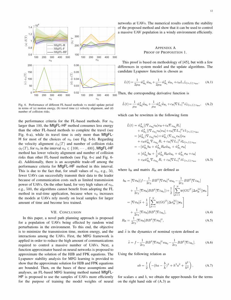
Fig. 6 shows the impact of model update period n0 on

12

Fig. 6. Performance of different FL-based methods vs model update periodin terms of (a) motion energy, (b) travel time (c) velocity alignment, and (d)number of collision risks.

the performance criteria for the FL-based methods. For n0

larger than 100, the MfgFL-HF method consumes less energythan the other FL-based methods to complete the travel (seeFig. 6-a), while its travel time is only more than MfgFL-H for most of the choices of n0 (see Fig. 6-b). Regardingthe velocity alignment φA(T ) and number of collision risksφC(T ), for n0 in the interval n0 ∈ 100, · · · , 400, MfgFL-HFmethod has lower velocity alignment and number of collisionrisks than other FL-based methods (see Fig. 6-c and Fig. 6-d). Additionally, there is an acceptable trade-off among theperformance criteria for MfgFL-HF method in this interval.This is due to the fact that, for small values of n0, e.g., 50,fewer UAVs can successfully transmit their data to the leaderbecause of communication costs such as limited transmissionpower of UAVs. On the other hand, for very high values of n0,e.g., 500, the algorithms cannot benefit from adopting the FLmethod in real-time application, because when n0 increasesthe models at UAVs rely mostly on local samples for largeramount of time and become less trained.

VII. CONCLUSION

In this paper, a novel path planning approach is proposedfor a population of UAVs being effected by random windperturbations in the environment. To this end, the objectiveis to minimize the transmission time, motion energy, and theinteractions among the UAVs. First, the MFG framework isapplied in order to reduce the high amount of communicationsrequired to control a massive number of UAVs. Next, afunction approximator based on neural networks is proposed toapproximate the solution of the HJB and FPK equations. TheLyapunov stability analysis for MFG learning is provided toshow that the approximate solution for HJB and FPK equationsare bounded. Then, on the bases of these assumptions andanalyses, an FL-based MFG learning method named MfgFL-HF is proposed to use the samples of UAVs more efficientlyfor the purpose of training the model weights of neural

networks at UAVs. The numerical results confirm the stabilityof the proposed method and show that it can be used to controla massive UAV population in a windy environment efficiently.

APPENDIX APROOF OF PROPOSITION 1.

This proof is based on methodology of [45], but with a fewdifferences in system model and the update algorithms. Thecandidate Lyapunov function is chosen as

L(t)=1

2µHwᵀ

H0wH0 +

1

2µHwᵀ

H1wH1 +cHLs1‖si‖≥sdest . (A.1)

Then, the corresponding derivative function is

L(t)=1

µHwᵀ

H0˙wH0 +

1

µHwᵀ

H1˙wH1 +cH[∇Ls]ᵀs1‖si‖≥sdest , (A.2)

which can be rewritten in the following form

L(t) = wᵀH0

[(∇wH0eH)eH+cH∇wH0

Ri]

+ wᵀH1

[(∇wH1eH)eH]+cH[∇Ls]ᵀs1‖si‖≥sdest

= [wᵀH0

(∇wH0eH)+wᵀ

H1(∇wH1

eH)]eH

+ cHwᵀH0∇wH0

Ri + cH[∇Ls]ᵀs1‖si‖≥sdest

= −[wᵀH0bH + wᵀ

H0RHwH0 + wᵀ

H1σH]

× [wᵀH0bH +

1

2wᵀ

H0RHwH0 + wᵀ

H1σH +εH]

+ cHwᵀH0∇wH0

Ri + cH[∇Ls]ᵀs1‖si‖≥sdest (A.3)

where bH and matrix RH are defined as

bH = [∇σH](f− 1

2c3BBᵀ[∇σH]ᵀwH0−

1

2c3BBᵀ[∇εH0 ]

+1

2c3[∇σH]BBᵀ[∇εH0 ])+

1

2

[N∑k=1

tr(GGT [∆σ[k]H ])ek

]

= [∇σH]¯s+1

2

[N∑k=1

tr(GGT [∆σ[k]H ])ek

]+

1

2c3[∇σH]BBᵀ[∇εH0 ], (A.4)

RH =1

2c3[∇σH]BBᵀ[∇σH]ᵀ, (A.5)

and ¯s is the dynamics of nominal system defined as

¯s = f− 1

2c3BBᵀ[∇σH]ᵀwH0−

1

2c3BBᵀ[∇εH0 ]. (A.6)

Using the following relation as

ab =1

2

(−(ha− b

h)2 + h2a2 +

b2

h2

), (A.7)

for scalars a and b, we obtain the upper-bounds for the termson the right hand side of (A.3) as

13

−3

2(wᵀ

H0bH)(wᵀ

H0RHwH0) ≤ 3

4h2

1λ21M‖wH0‖

2+3

4h21

λ22M‖wH0‖

4,

(A.8)

−(wᵀH0bH)(εH) ≤ 1

2h2

2λ21M‖wH0‖

2 +1

2h22

λ23M , (A.9)

−(wᵀH0RHwH0)(εH) ≤ 1

2h2

3λ22M‖wH0‖

4 +1

2h23

λ23M ,

(A.10)

−3

2(wᵀ

H1σH)(wᵀ

H0RHwH0) ≤ 3

4h2

4λ24M‖wH1‖

2 +3

4h24

λ22M‖wH0‖

4,

(A.11)

−(wᵀH1σH)(εH) ≤ 1

2h2

5λ24M‖wH1‖

2 +1

2h25

λ23M ,

(A.12)

−2(wᵀH0bH)(wᵀ

H1σH) ≤ h2

6λ21M‖wH0‖

2 +1

h26

λ24M‖wH1‖

2,

(A.13)

−(wᵀH0bH)2 ≤ −λ2

1m‖wH0‖2, (A.14)

−1

2(wᵀ

H0RHwH0)2 ≤ −1

2λ2

2m‖wH0‖4, (A.15)

−(wᵀH1σH)2 ≤ −λ2

4m‖wH1‖2, (A.16)

where we assumed that

λ1m ≤ ‖bH‖ ≤ λ1M , (A.17)λ2m ≤ ‖RH‖ ≤ λ2M , (A.18)

‖εH‖ ≤ λ3M , (A.19)λ4m ≤ ‖σH‖ ≤ λ4M . (A.20)

Therefore, the derivative of Lyapunov function is upper-bounded as

L(t) ≤ −λ0‖wH0‖4 + λ1‖wH0‖

2 + λ22 − λ3‖wH1‖

2

+ cHwᵀH0∇wH0

Ri + cH[∇Ls]ᵀs1‖si‖≥sdest , (A.21)

where λ0, λ1, λ2, and λ3 are defined as

λ0 = − 3

4h21

λ22M −

1

2h2

3λ22M −

3

4h24

λ22M +

1

2λ2

2m,

λ1 =3

4h2

1λ21M +

1

2h2

2λ21M + h2

6λ21M − λ2

1m,

λ3 = −3

4h2

4λ24M −

1

2h2

5λ24M −

1

h26

λ24M + λ2

4m,

λ22 =

1

2h22

λ23M +

1

2h23

λ23M +

1

2h25

λ23M . (A.22)

Depending on the state of the UAV, three cases can occurin (A.21) as

Case 1: 1‖si‖≥sdest = 0. With this condition, we can concludethat the UAVs are in destination, and we focus only on theweights of the models

L(t) ≤ −λ0‖wH0‖4 + λ1‖wH0‖

2 + λ22 − λ3‖wH1‖

2. (A.23)

Then, when the following conditions hold, i.e.,

‖wH0‖ ≥

√λ1 +

√λ2

1 + 4λ0λ22

2λ0=∆ ω0,1, (A.24)

‖wH1‖ ≥

√4λ2

2λ0 + λ21

4λ3λ0=∆ ω1,1, (A.25)

the stability condition L(t) < 0 is satisfied.

case 2: 1‖si‖≥sdest = 1 and Ls ≤ 0. In this case, theregulizer term is inactive, and the upper-bound for derivativeof Lyapunov is reduced to

L(t) ≤ −λ0‖wH0‖4 + λ1‖wH0‖

2 + λ22 − λ3‖wH1‖

2

+ cH[∇Ls]ᵀs1(‖si‖≥sdest)

≤ −λ0‖wH0‖4 + λ1‖wH0‖

2 + λ22 − λ3‖wH1‖

2

+ cHλ4‖∇Ls‖ (A.26)

where λ4 is a number such that 0 < λ4‖∇Ls‖ ≤ −[∇Ls]ᵀs .Therefore, when the following inequalities as

‖wH0‖ ≥

√λ1 +

√λ2

1 + 4λ0λ22

2λ0=∆ ω0,2 (A.27)

‖wH1‖ ≥

√4λ2

2λ0 + λ21

4λ3λ0=∆ ω1,2 (A.28)

‖∇Ls(si(t))‖ ≥4λ2

2λ0 + λ21

4λ4λ0=∆ γ2 (A.29)

occur, the stability condition L(t) < 0 holds.case 3: 1‖si‖≥sdest = 1 and Ls ≥ 0. In this case, we find the

upper-bound for the L(t) as

L(t) ≤ −λ0‖wH0‖4 + λ1‖wH0‖

2 + λ22 − λ3‖wH1‖

2

+ cHwᵀH0∇wH0

Ri + cH[∇Ls]ᵀs1‖si‖≥sdest

= −λ0‖wH0‖4 + λ1‖wH0‖

2 + λ22 − λ3‖wH1‖

2

+ cHwᵀH0∇wH0

[[∇Ls]ᵀs] + cH[∇Ls]ᵀs(1)= −λ0‖wH0‖

4 + λ1‖wH0‖2 + λ2

2 − λ3‖wH1‖2

+ cH[∇Ls]ᵀ ¯s+cH

2c3[∇Ls]ᵀBBᵀ[∇εH0 ]

(2)

≤ −λ0‖wH0‖4 + λ1‖wH0‖

2 + λ22 − λ3‖wH1‖

2

− cHλ5m‖∇Ls‖2 +cH

2c3λ6M‖∇Ls‖, (A.30)

where equality (1) is obtained by the calculations as

cHwᵀH0∇wH0

[[∇Ls]ᵀs] =1

2c3cH[wH0 ]ᵀ[∇σH]BBᵀ[∇Ls], (A.31)

cH[∇Ls]ᵀs = cH[∇Ls]ᵀ(f − 1

2c3BBᵀ[∇σH]ᵀwH0), (A.32)

and inequality (2) is based on the following assumptions,

[∇Ls]ᵀ ¯s = −[∇Ls]ᵀA[∇Ls], (A.33)

≤ −λ5m‖∇Ls‖2, (A.34)

BBᵀ[∇εH0 ] ≤ λ6M . (A.35)

where λ5m is the minimum eigenvalue of matrix A.Therefore, when the following conditions occur, i.e.,

‖wH0‖ ≥

√√√√√λ1 +

√λ2

1 + 4λ0(λ22 +

cHλ26M

16c23λ5m)

2λ0=∆ ω0,3

(A.36)

‖wH1‖ ≥

√√√√4(λ22 +

cHλ26M

16c23λ5m)λ0 + λ2

1

4λ3λ0=∆ ω1,3 (A.37)

‖∇Ls(si(t))‖ ≥cH2c3

λ6M+

√( cH

2c3λ6M )2+4cHλ5m(λ2

2+λ21

4λ0)

cHλ5m=∆ γ3

(A.38)

the Lyapunov stability condition holds, i.e., L(t) < 0.

14

In summary, when ‖wH0‖ ≥ ω0 = maxω0,1, ω0,2, ω0,3,

or ‖wH1‖ ≥ ω1 = maxω1,1, ω1,2, ω1,3, or ‖∇Ls(si(t))‖ ≥

maxγ2, γ3 occurs, then the Lyapunov stability conditionholds, i.e., L(t) < 0. Considering all the cases 1-3, we canconclude that there exist sdest, w0, and w1 at time T such that‖s(t)‖ ≤ sdest, ‖wH0(t) − wH0(t)‖ ≤w0, and ‖wH1(t) − wH1(t)‖ ≤w1 for all t ≥ T + T ′.

APPENDIX BPROOF OF PROPOSITION 2.

The candidate Lyapunov function is chosen as

L(t) =1

2µFwᵀ

F0wF0 +

1

2µFwᵀ

F1wF1 . (B.1)

Then, the derivative of Lyapunov function is obtained as

L(t) = wᵀF0

(∇wF0eF)eF + wᵀ

F1(∇wF1

eF)eF,

= −[wᵀF0

[∇wF0eF] + wᵀ

F1[∇wF1

eF]],

[wᵀF0

[∇wF0eF] + wᵀ

F1[∇wF1

eF] + εF],

= −[wᵀF [∇wFeF]][wᵀ

F [∇wFeF] + εF]. (B.2)

Each term of the derivative of Lyapunov function has an upper-bound obtained as

−(wᵀF∇wFeF)2 ≤ −λ2

7m‖wF‖2, (B.3)

−(wᵀF [∇wFeF])(εF) ≤ λ8Mλ7M‖wᵀ

F‖, (B.4)

where it is assumed that

λ7m ≤ ‖∇wFeF‖ ≤ λ7M , (B.5)‖εF‖ ≤ λ8M . (B.6)

Then, the derivative of Lyapunov is upper-bounded as

L(t) ≤ −λ27m‖wF‖2 + λ8Mλ7M‖wᵀ

F‖. (B.7)

Therefore, when the following condition occurs, i.e.,

‖wᵀF‖ ≥

λ8Mλ7M

λ27m

, (B.8)

the stability condition holds, i.e., L(t) ≤ 0. However, (B.8)means that the model which makes the term ‖εF‖ small, canincrease the stability of FPK learning algorithm.

APPENDIX CPROOF OF PROPOSITION 3.

Here we aim to show the convergence and bias of the FPKlearning updates following the proof method of [46]. Let usfirst define extended vectors as

wF(n) = [[wF0(n)]ᵀ [wF1(n)]ᵀ]ᵀ, (C.1)wF(n) = [[wF0(n)]ᵀ [wF1(n)]ᵀ]ᵀ, (C.2)∇wFeF = [[∇wF0

eF]ᵀ [∇wF1eF]ᵀ]ᵀ. (C.3)

Then, the FPK error vector update is obtained as

wF(n+1)=[I−µF[∇wFeF][∇wFeF]ᵀ]wF(n)− µF[∇wFeF]εF.(C.4)

A. FPK Mean Stability

Taking the expectation of equation (C.4) yields

E[wF(n+1)] = [I−µFE[[∇wFeF][∇wFeF]ᵀ]]E[wF(n)]

− µFE[[∇wFeF]εF], (C.5)

We can assume that the vector [∇wFeF] which depends on theinputs, and εF which depends on the neural network design,are independent. Then we can write

E[[∇wFeF]εF] = 0. (C.6)

Let us define the matrix R as

R =∆ E[[∇wFeF][∇wFeF]ᵀ]. (C.7)

By substituting (C.6) and (C.7) in equation (C.5), it can berewritten in the form

E[wF(n+1)] = [I − µFR]E[wF(n)]. (C.8)

Then, the necessary condition for the convergence of thisequation is

0 < µF <2

λmax, (C.9)

where λmax is the largest eigenvalue of the matrix R.

B. Biasness

Assuming small step-sizes and also the condition (C.9), thebias of estimation is calculated as

bias = limn→∞

−E[wF(n)] = 0, (C.10)

which means that if the step size is small enough such thatthe convergence condition holds, the parameters of the FPKequation tend to its optimal values.

C. Mean Square Convergence Analysis

The mean square deviation (MSD) of the estimation algo-rithm is defined as

MSDF = limn→∞

E[‖wF(n)‖2]. (C.11)

In order to find the MSD, let us first define the weighted MSDof the algorithm as E[‖wF(n)‖2Σ], which can be obtained bythe recursive equation

E[‖wF(n+ 1)‖2Σ] = E[‖wF(n)‖2Σ

′ ] + µ2Ftr(RΣ)‖εF‖2, (C.12)

where Σ is a positive definite matrix, and

Σ′ = (I − µFR)ᵀΣ(I − µFR), (C.13)RΣ = E[[∇wFeF]ᵀΣ[∇wFeF]]. (C.14)

We know that tr(ΣX) = [vec(X)]ᵀσ, and vec(UΣV ) =(V ᵀ ⊗ U)σ, where vec(·) is a vectorazation operator, i.e.,vec(Σ) = σ. Using these equalities, we can obtain

tr(RΣ) = [vec(R)]ᵀσ, (C.15)

σ′ = Fσ, (C.16)F = (I − µFR)ᵀ ⊗ (I − µFR)ᵀ. (C.17)

At the convergence stage, the MSD is written as

limn→∞

E[‖wF(n)‖2Ω] = µ2F‖εF‖2[vec(R)]ᵀ(I −F)−1vec(Ω),

(C.18)

15

where vec(Ω) = (I − F)σ Therefore the steady state MSD isobtained as

MSDF = µ2F‖εF‖2[vec(R)]ᵀ(I −F)−1vec(I), (C.19)

The value of MSD can be very small by choosing a smallvalue for step sizes, i.e., µF, and choosing a model whichmakes ‖εF‖ small.

REFERENCES

[1] H. Kim, J. Park, M. Bennis, and S.-L. Kim, “Massive UAV-to-groundcommunication and its stable movement control: A mean-field ap-proach,” in Proc. IEEE SPAWC, Kalamata, Greece, Jun. 2018.

[2] E. Ackerman and E. Strickland, “Medical delivery drones take flight ineast africa,” IEEE Spectrum, vol. 55, no. 1, pp. 34–35, Jan. 2018.

[3] J. Tisdale, Z. Kim, and J. K. Hedrick, “Autonomous UAV path planningand estimation,” IEEE Robot. Autom. Mag., vol. 16, no. 2, pp. 35–42,Jun. 2009.

[4] H. Shiri, J. Park, and M. Bennis, “Massive autonomous UAV pathplanning: A neural network based mean-field game theoretic approach,”arXiv preprint arXiv:1905.04152, 2019.

[5] M. Huang, R. P. Malhame, P. E. Caines et al., “Large populationstochastic dynamic games: closed-loop mckean-vlasov systems and thenash certainty equivalence principle,” Communications in Information& Systems, vol. 6, no. 3, pp. 221–252, 2006.

[6] M. Huang, P. E. Caines, and R. P. Malhame, “Large-population cost-coupled lqg problems with nonuniform agents: individual-mass behaviorand decentralized n -nash equilibria,” IEEE transactions on automaticcontrol, vol. 52, no. 9, pp. 1560–1571, 2007.

[7] J.-M. Lasry and P.-L. Lions, “Mean field games,” Japanese journal ofmathematics, vol. 2, no. 1, pp. 229–260, 2007.

[8] H. B. McMahan, E. Moore, D. Ramage, S. Hampson et al.,“Communication-efficient learning of deep networks from decentralizeddata,” arXiv preprint arXiv:1602.05629, 2016.

[9] R. Shokri and V. Shmatikov, “Privacy-preserving deep learning,” inProceedings of the 22nd ACM SIGSAC conference on computer andcommunications security, 2015, pp. 1310–1321.

[10] D. Liu, D. Wang, F. Wang, H. Li, and X. Yang, “Neural-network-based online hjb solution for optimal robust guaranteed cost controlof continuous-time uncertain nonlinear systems,” IEEE Transactions onCybernetics, vol. 44, no. 12, pp. 2834–2847, Dec 2014.

[11] H. Shiri, J. Park, and M. Bennis, “Remote uav online path plan-ning via neural network based opportunistic control,” arXiv preprintarXiv:1910.04969, 2019.

[12] A. Kavvadias, E. Psomiadis, M. Chanioti, E. Gala, and S. Michas,“Precision agriculture-comparison and evaluation of innovative very highresolution (uav) and landsat data.” in HAICTA, 2015, pp. 376–386.

[13] T. Tomic, K. Schmid, P. Lutz, A. Domel, M. Kassecker, E. Mair,I. L. Grixa, F. Ruess, M. Suppa, and D. Burschka, “Toward a fullyautonomous uav: Research platform for indoor and outdoor urban searchand rescue,” IEEE robotics & automation magazine, vol. 19, no. 3, pp.46–56, 2012.

[14] H. X. Pham, H. M. La, D. Feil-Seifer, and L. V. Nguyen, “Au-tonomous uav navigation using reinforcement learning,” arXiv preprintarXiv:1801.05086, 2018.

[15] J. Chen, T. Liu, and S. Shen, “Online generation of collision-freetrajectories for quadrotor flight in unknown cluttered environments,”in 2016 IEEE International Conference on Robotics and Automation(ICRA). IEEE, 2016, pp. 1476–1483.

[16] B. Allred, N. Eash, R. Freeland, L. Martinez, and D. Wishart, “Effectiveand efficient agricultural drainage pipe mapping with uas thermalinfrared imagery: A case study,” Agricultural Water Management, vol.197, pp. 132–137, 2018.

[17] R. Jannoura, K. Brinkmann, D. Uteau, C. Bruns, and R. G. Joergensen,“Monitoring of crop biomass using true colour aerial photographs takenfrom a remote controlled hexacopter,” Biosystems Engineering, vol. 129,pp. 341–351, 2015.

[18] P. J. Zarco-Tejada, M. L. Guillen-Climent, R. Hernandez-Clemente,A. Catalina, M. Gonzalez, and P. Martın, “Estimating leaf carotenoidcontent in vineyards using high resolution hyperspectral imagery ac-quired from an unmanned aerial vehicle (uav),” Agricultural and forestmeteorology, vol. 171, pp. 281–294, 2013.

[19] D. Rathbun, S. Kragelund, A. Pongpunwattana, and B. Capozzi, “Anevolution based path planning algorithm for autonomous motion of auav through uncertain environments,” in Proceedings. The 21st DigitalAvionics Systems Conference, vol. 2. IEEE, 2002, pp. 8D2–8D2.

[20] Y. Zeng and R. Zhang, “Energy-efficient uav communication with tra-jectory optimization,” IEEE Transactions on Wireless Communications,vol. 16, no. 6, pp. 3747–3760, 2017.

[21] H. Inaltekin, M. Gorlatova, and M. Chiang, “Virtualized control overfog: interplay between reliability and latency,” IEEE Internet of ThingsJournal, vol. 5, no. 6, pp. 5030–5045, 2018.

[22] D. Doering, A. Benenmann, R. Lerm, E. P. de Freitas, I. Muller, J. M.Winter, and C. E. Pereira, “Design and optimization of a heterogeneousplatform for multiple uav use in precision agriculture applications,” IFACProceedings Volumes, vol. 47, no. 3, pp. 12 272–12 277, 2014.

[23] G. Vasarhelyi, C. Viragh, G. Somorjai, T. Nepusz, A. E. Eiben, andT. Vicsek, “Optimized flocking of autonomous drones in confinedenvironments,” Science Robotics, vol. 3, no. 20, 2018. [Online].Available: http://robotics.sciencemag.org/content/3/20/eaat3536

[24] C. Ju and H. Son, “Multiple uav systems for agricultural applications:control, implementation, and evaluation,” Electronics, vol. 7, no. 9, p.162, 2018.

[25] M. Nourian, P. E. Caines, and R. P. Malhame, “Mean field analysis ofcontrolled cucker-smale type flocking: Linear analysis and perturbationequations,” IFAC Proceedings Volumes, vol. 44, no. 1, pp. 4471–4476,2011.

[26] K. W. Morton and D. F. Mayers, Numerical solution of partial differ-ential equations: an introduction. Cambridge university press, 2005.

[27] S. Khardi, “Aircraft flight path optimization. the hamilton-jacobi-bellman considerations,” Applied Mathematical Sciences, vol. 6, no. 25,pp. pp–1221, 2012.

[28] C. Greif, “Numerical methods for hamilton-jacobi-bellman equations,”2017.

[29] Y. Tassa and T. Erez, “Least squares solutions of the hjb equation withneural network value-function approximators,” IEEE transactions onneural networks, vol. 18, no. 4, pp. 1031–1041, 2007.

[30] B. Luo, H.-N. Wu, T. Huang, and D. Liu, “Reinforcement learningsolution for hjb equation arising in constrained optimal control problem,”Neural Networks, vol. 71, pp. 150–158, 2015.

[31] A. Faust, P. Ruymgaart, M. Salman, R. Fierro, and L. Tapia, “Continuousaction reinforcement learning for control-affine systems with unknowndynamics,” IEEE/CAA Journal of Automatica Sinica, vol. 1, no. 3, pp.323–336, 2014.

[32] J. W. Kim, B. J. Park, H. Yoo, J. H. Lee, and J. M. Lee, “Deepreinforcement learning based finite-horizon optimal tracking control fornonlinear system,” IFAC-PapersOnLine, vol. 51, no. 25, pp. 257–262,2018.

[33] C. Beck, S. Becker, P. Grohs, N. Jaafari, and A. Jentzen, “Solvingstochastic differential equations and Kolmogorov equations by meansof deep learning,” arXiv e-prints, p. arXiv:1806.00421, Jun 2018.

[34] H. M. La, “Multi-robot swarm for cooperative scalar field mapping,”in Handbook of Research on Design, Control, and Modeling of SwarmRobotics. IGI Global, 2016, pp. 383–395.

[35] H. M. La, W. Sheng, and J. Chen, “Cooperative and active sensing inmobile sensor networks for scalar field mapping,” IEEE Transactionson Systems, Man, and Cybernetics: Systems, vol. 45, no. 1, pp. 1–12,2015.

[36] P. Sujit, S. Saripalli, and J. B. Sousa, “Unmanned aerial vehicle pathfollowing: A survey and analysis of algorithms for fixed-wing unmannedaerial vehicless,” IEEE Control Systems Magazine, vol. 34, no. 1, pp.42–59, 2014.

[37] W. Koch, R. Mancuso, R. West, and A. Bestavros, “Reinforcementlearning for uav attitude control,” arXiv preprint arXiv:1804.04154,2018.

[38] C. Richter, W. Vega-Brown, and N. Roy, “Bayesian learning for safehigh-speed navigation in unknown environments,” in Robotics Research.Springer, 2018, pp. 325–341.

[39] O. Gueant, J.-M. Lasry, and P.-L. Lions, “Mean field games andapplications,” in Paris-Princeton lectures on mathematical finance 2010.Springer, 2011, pp. 205–266.

[40] N. Goddemeier and C. Wietfeld, “Investigation of air-to-air channelcharacteristics and a uav specific extension to the rice model,” in 2015IEEE Globecom Workshops (GC Wkshps), Dec 2015, pp. 1–5.

[41] R. Zarate-Minano, F. M. Mele, and F. Milano, “SDE-based wind speedmodels with Weibull distribution and exponential autocorrelation,” inProc. IEEE PESGM, Boston, MA, USA, 2016.

[42] F. Cucker and J.-G. Dong, “Avoiding collisions in flocks,” IEEE Trans-actions on Automatic Control, vol. 55, no. 5, pp. 1238–1243, 2010.

16

[43] Z. Lin, M. Broucke, and B. Francis, “Local control strategies for groupsof mobile autonomous agents,” IEEE Transactions on automatic control,vol. 49, no. 4, pp. 622–629, 2004.

[44] N. Goddemeier and C. Wietfeld, “Investigation of air-to-air channelcharacteristics and a uav specific extension to the rice model,” in 2015IEEE Globecom Workshops (GC Wkshps), Dec 2015, pp. 1–5.

[45] D. Liu, D. Wang, F.-Y. Wang, H. Li, and X. Yang, “Neural-network-

based online HJB solution for optimal robust guaranteed cost controlof continuous-time uncertain nonlinear systems,” IEEE Trans. Cybern.,vol. 44, no. 12, pp. 2834–2847, Dec. 2014.

[46] H. Shiri, M. A. Tinati, M. Codreanu, and S. Daneshvar, “Distributedsparse diffusion estimation based on set membership and affine projec-tion algorithm,” Digital Signal Processing, vol. 73, pp. 47–61, 2018.