Communication Constrained Trajectory AlignmentFor Multi-Agent Inspection via Linear Programming

Joshua G. Mangelson, Ram Vasudevan, and Ryan M. Eustice

Abstract— This paper reports on a system for estimatingthe alignment between robotic trajectories under constrainedcommunications. Multi-agent collaborative inspection and nav-igation tasks depend on the ability to determine an alignmentbetween robotic trajectories or maps. The properties of theunderwater environment make determining such an alignmentdifficult because of extreme limitations on communication andthe lack of absolute position measurements such as GPS.In this paper, we propose a method that takes advantageof convex relaxation techniques to determine an alignmentbetween robotic trajectories based on sparse observations ofa low-dimensional underlying feature space. We use a linearapproximation of the l2-norm to approximately enforce that theestimated transformation is an element of SO(2). Because therelaxed optimization problem is linear, we can take advantageof existing convex optimization libraries, which do not requirean initial estimate of relative pose. In addition, because theproposed method does not need to perform data association, wecan align trajectories using low-dimensional feature vectors andcan thus decrease the amount of data that must be transferredbetween agents by several orders of magnitude when comparedto image feature descriptors such as SIFT and SURF. Weevaluate the proposed method on simulated datasets and applyit to real-world data collected during autonomous ship hullinspection field trials.

I. INTRODUCTION

Multi-agent underwater inspection and mapping tasks de-pend on the ability to determine an alignment betweenmultiple robot maps or trajectories. This is challenging inunderwater environments where global positioning systemsare unavailable and where acoustic positioning systems re-quire extensive setup and calibration [1]. Moreover, in fullysubmersed scenarios, communication is limited to a fewbits per second making data transfer a significant systemconstraint [2].

Existing methods for estimating this alignment rely onthe matching of discrete feature points observed by mul-tiple robotic vehicles [3]. However, performing this dataassociation requires that feature points transfer-ed betweenagents be uniquely identifiable. This is usually accomplishedthrough the transfer of high dimensional feature descriptionsthat often surpass the throughput available in the underwaterenvironment.

This paper proposes a method that efficiently estimatesthe rigid body transformation between reference and query

*This work was supported by the Office of Naval Research under awardN00014-16-1-2102;

J. Mangelson, R. Vasudevan, and R. Eustice are with the RoboticsInstitute at the University of Michigan. R. Vasudevan is also with theDepartment of Mechanical Engineering and R. Eustice is with the De-partment of Naval Architecture and Marine Engineering. {mangelso,ramv, eustice}@umich.edu.

Fig. 1: An overview of the proposed trajectory alignment algorithm.Given sparse observations of an underlying feature space, weformulate a linear optimization problem that seeks to align a querytrajectory with a reference trajectory. We do this by iterativellycreating a linear cost that minimizes feature distance and optimizingover the transformation that minimizes that cost.

robot trajectories based on a sparsely sampled underlyingfeature space. Because we formulate the problem as a convexoptimization problem, our method avoids performing dataassociation and decreases the amount of data that needs tobe transferred between robotic vehicles by several orders ofmagnitude. In addition, because our formulation is convex,our proposed method is not dependent on initialization anddoes not require a prior estimate of the relative transforma-

tion between trajectories. Finally, our method is paralleliz-able and takes advantage of existing commercial optimiza-tion libraries to increase the efficiency of the optimizationprocess.

The contributions of this paper include the following:1) The development of a system for alignment and local-

ization of robot trajectories that:i) Relies only on low-dimensional feature observations.ii) Avoids performing data association.iii) Does not require an initial alignment estimate.

2) A novel linear approximation based method for ap-proximate optimization over SO(2).

3) A parallelized implementation of the proposed method.The remainder of this paper is organized as follows:

In §II, we provide an overview of related areas of work.In §III we formalize the trajectory alignment problem. In§IV, we present a method that takes advantage of convexrelaxation techniques to generate a linear cost function thatis minimized when query feature points are placed near ref-erence feature points with similar value. In §V, we present anovel method that uses linear programming to approximatelyoptimize over SO(2). In §VI, we provide an outline of thefull system and our released implementation. We evaluate theproposed algorithm on simulated datasets in §VII and applyit to multi-agent ship hull inspection in §VIII. Finally, weconclude in §IX.

II. RELATED WORK

Multi-agent collaborative mapping has been heavily re-searched and a variety of methods have been developedfor estimating the relative transformation between robotcoordinate frames. Early methods assumed that vehicles wereable to observe one another directly [4–6]. These methodsrelied on a single direct observation to determine the relativepose (position and orientation) of the two agents. Later,maximum likelihood based simultaneous localization andmapping (SLAM) methods enabled the use of multiple ob-servations by estimating the most likely alignment and mapgiven all the observed measurements [7–11]. These methodsoften relax the assumption that vehicles must be able toobserve one another directly. Instead, features present inthe environment observed by both vehicles are co-registeredand used to relate the pose of the two vehicles. Mostrecent methods for determining multi-agent alignment arebased on co-registering data in this way [3, 12–14]. Whileco-registering observed data works well in many cases, itdepends on the ability to transmit large amounts of databetween vehicles. This work focuses on developing methodsthat minimize the amount of data that must be transmittedbetween agents.

Our work is also related to research in the area of terrainbased navigation [15–17]. In the underwater environment,this refers the use of a known bathymetric map of the seafloorto improve navigation estimates. These methods, however,are more focused on improving the estimate of a singlerobot’s trajectory than on determining the alignment betweenmultiple trajectories. In addition, these methods require an a

prioi map of the environment, while our ultimate goal is todirectly align the trajectories of two robotic vehicles that aresimultaneously performing an inspection/mapping task in apotentially unknown environment.

There has also been significant recent interest in the SLAMand computer vision communities in developing estimationalgorithms that leverage convex optimization techniques toavoid the need for an initial guess [14, 18–21]. This isespecially useful in the underwater environment where globalpositioning system (GPS) is not available and global mea-surements of position can be hard to come by. In 2014, Liet al. [21] proposed a method that uses the convex hull ofa set of dissimilarity points to estimate the affine transfor-mation that must have occurred to transform a set of pointsobserved in one image to a similar set of points observed inanother. Their proposed method results in a linear (convex)cost function that can take advantage of existing optimizationlibraries and does not require an initialization. However,to apply their method to the trajectory alignment problem,we need to ensure that the estimated trajectory is rigid asopposed to affine.

Optimization over the group of rigid body transformationsis generally non-convex making it hard to guarantee the trueoptimum. Recent works have investigated convex relaxationbased methods for performing optimization over the groupof rigid body transformations (the special euclidean groupSE(d)) [18, 19]. Specifically, these methods relax optimiza-tion over the set of valid rotation matrices SO(d) to opti-mization over the convex hull of SO(d). These methods workwell in many cases. However, they fail to enforce that theestimated transformation be a valid rigid body transforma-tion. The optimization problem used in our method also takesadvantage of convex relaxation techniques, however, we usea linear approximation of the `2-norm to add an additionalset of constraints to the optimization that collectively enforcethat the estimated transformation be approximately rigid.This results in more accurate transformation estimates thanoptimization over the convex hull of SO(d).

III. PROBLEM FORMULATION

In this section, we outline the need for communicationconstrained trajectory alignment in underwater inspectionand then formalize the trajectory alignment problem.

A. Trajectory Alignment w/o Data Association

In multi-agent inspection tasks, multiple vehicles navigatethrough the environment collecting information and estimat-ing a map of the structure or scene they are inspecting.Some form of these local maps are then transmitted betweenvehicles allowing the agents to use the data collected byother vehicles for navigation, path planning, or global mapgeneration. However, before an agent can use the data col-lected by another agent, it must first determine an alignmentbetween its own local trajectory/map and the trajectory/mapreceived from the other agent. Traditionally, this alignmentis determined by matching locations in the environmentobserved by both agents [4–6].

However, communicating large amounts of data suchas point clouds or high-dimensional image feature vectorsbetween vehicles is often not practical in the underwaterdomain. While one approach is to limit data transfer byprioritizing data that is most likely to be useful, our approachis to cut out the transfer of this high-dimensional datacompletely. Instead, we take a descretized version of therobot trajectory and summarize information observed neareach individual robot position using a small low-dimensionalfeature vector. We then align the robot trajectories by tryingto find a rigid body transformation that places poses withsimilar descriptions near one another, without trying to matchindividual features. Taking this approach allows us to limitthe data that must be transferred between vehicles to thediscretized set of positions and the associated set of low-dimensional feature vectors.

B. Convex Trajectory Alignment

Formally, our goal is to align a query trajectory with areference trajectory based only on low dimensional featurevectors describing the environment at each position visitedby the two trajectories.

We denote the positions visited by the reference trajectoryby {pa

1 , · · · ,pana} and the associated feature vectors by

{ξa1 , · · · , ξana}, indexed by i. Similarly, the query trajectory

positions and feature vectors are denoted by {pb1, · · · ,pb

nb}

and {ξb1, · · · , ξbnb}, respectively, indexed by j. We then frame

the trajectory alignment problem as an optimization thatseeks to find a transformation that transforms positions in thecoordinate frame of the query trajectory into the coordinateframe of the reference trajectory, such that when the points{pb

1, · · · ,pbnb} are transformed they lie nearby points in

{pa1 , · · · ,pa

na} with similar feature values. Thus, the feature

vectors ξ only need to describe the local environment asopposed to uniquely identify a specific point and can, as aresult, have a much lower dimension.

Using a formulation similar to [21], we define a trans-formation function T ab

j (Θ) : Rn 7→ Rd that maps the j-thquery point, pb

j , to a position represented with respect to thereference trajectory coordinate frame. Specifically, we defineT abj (Θ) as

T abj (Θ) = Rabpb

j + tab, (1)

where Θ = (Rab, tab) are the parameters of the function.Together, Rab ∈ SO(d) and tab ∈ Rd parameterize a globalrigid body transformation relating the local coordinate framesof the two vehicles. The points pb

j are fixed in the functionT abj and we thus define nb transformation functions, one for

each feature in the query trajectory.We also define a function cj : Rd 7→ R that takes a

position represented in the reference trajectory coordinateframe, pa ∈ Rd, and calculates the feature dissimilaritybetween ξbj and the given position. As before, becausethere are nb query feature points, we define nb differentdissimilarity functions cj , j = 1, · · · , nb. §IV provides moredetail on how these functions are defined.

With these definitions, we can formulate the final overallobjective function as follows:

minimizeRab∈SO(d)

tab∈Rd

nb∑j=1

cj(Tabj (Θ)) (2)

where cj(Tabj (Θ)) is the dissimilarity between the feature

vector ξbj and its new transformed position in the referencetrajectory coordinate frame. Solving this optimization prob-lem would allow us to find the transformation that minimizesthe dissimilarity between query feature points and theirassociated positions in the reference trajectory coordinateframe.

Note, that while our formulation is based on that of [21],their method assumes the transformation is affine, while werestrict it to be an isometric (or rigid body [22]) transforma-tion. This assumption on their part, results in the associatedterms of their cost function being affine and the resultingoptimization problem being convex. However, when dealingwith physical transformations between coordinate frames, anaffine transformation does not represent reality and a rigidbody transformation must be used. This makes our resultingoptimization problem non-convex and more difficult to solve.In §V we explain a novel method to approximately optimizeover SO(2).

IV. CONVEX TRANSFORMATION ESTIMATIONVIA THE LOWER CONVEX HULL

In this section, we discuss the formulation of the dissim-ilarity functions cj , j = 1, · · · , nb that measure the featuredissimilarity of the feature vector ξbj and a position in thereference trajectory coordinate frame. We then compose thedissimilarity functions cj with the transformation function(1) so that we can optimize over the transformation param-eters as opposed to individual pose positions. There are twocases that we cover:

1) The 2D case where both maps lie in a 2D world(d = 2)2) The known depth case where both maps lie in the 3D

world(d = 3), but one coordinate is known.

We first cover the 2D case which follows directly from [21].We then generalize this to the case with known depth.

A. Convex Dissimilarity Function Definition in 2D

Following [21], we denote the feature dissimilarity be-tween ξai and ξbj by Cab

ij . If we use every possibly pairing,there are na×nb of these values and they can be calculatedbefore performing registration via an arbitrary dissimilarityfunction. However, because we want to find a transformationas opposed to a discrete matching, we create nb continuousand convex feature dissimilarity functions cj , j = 1, · · · , nb.Each cj takes a position represented with respect to thereference trajectory coordinate frame and returns a predictedlower bound on the dissimilarity of that position with respectto the feature vector ξbj . We derive this function by taking

the lower convex hull of the following point cloud:xa1 ya1 Cab

1j

xa2 ya2 Cab2j

......

...xana

yanaCab

naj

. (3)

For a given feature vector ξbj with d = 2, the point cloud (3)defines discrete points in a space that relates 2D positions inthe reference trajectory coordinate frame to their associateddissimilarity value with respect to ξbj . Because this space is3D, we can calculate the convex hull of these points usingan algorithm like [23]. The lower convex hull with respectto the dissimilarity value dimension is made up of a set ofplanes (facets) that represent lower bounds on the discretedissimilarity values Cab

ij for a given fixed j. These planescan be found by selecting the planes that have normal vectorswith a negative component in the dimension corresponding todissimilarity. Assuming there are Mj planes in the lower con-vex hull for feature ξbj , we can define these planes using theequations amx+bmy+cmCm+dm = 0, for m = 1, · · · ,Mj ,where x and y correspond to the position dimensions and Cm

corresponds to the dissimilarity dimension in the point cloud(3). We then rearrange these equations to arrive at the planefunctions Cm = rmx+ smy + tm, for m = 1, · · · ,Mj thatcalculate the predicted dissimilarity given a specified featureposition. Finally, we can now define the feature dissimilarityfunction cj as

cj([x, y]>) = max

m(rmx+ smy + tm), m = 1, · · · ,Mj .

(4)

This function is both continuous and convex and itsminimization can be transformed into an equivalent linearprogram [24]:

minimizeuj ,x,y

uj

subject to rmx+ smy + tm ≤ uj ,m = 1, · · · ,Mj .

(5)

Using the dissimilarity function (4) and the linear program(5) enables us to efficiently solve for an arbitrary 2D position[x, y]> ∈ R2 that minimizes the dissimilarity with respect toξbj for a given value of j. The next section describes howto compose cj( · ) with the transformation T ab

j (Θ) whichenables us to optimize over the parameters Θ = (Rab, tab).

B. Composition with the Transformation Function

Our goal is to estimate the rigid body transformationbetween respective trajectories. As such, rather than estimatethe individual locations of points, we estimate the parametersof the transformation, Θ, or more specifically the parametersRab and tab. We do this by minimizing cj(T ab

j (Θ)), for allj = 1, · · · , nb, as opposed to cj([x, y]>) directly.

Remembering that T abj (Θ) ∈ Rd represents the trans-

formed coordinates of pbj , we represent the function that

calculates the first coordinate of T abj (Θ) by fj(Θ) and the

second coordinate by gj(Θ). Specifically, define

fj(Θ) = Rab(1)pbj + tab(1) (6)

and

gj(Θ) = Rab(2)pbj + tab(2), (7)

where the notation (i) denotes the i-th row of the given matrixor vector and again pb

j is fixed for both fj and gj .Using this, we can rewrite (5) to be a minimization of

cj(Tabj (Θ)) over Θ as

minimizeuj∈R

Rab∈SO(2)

tab∈R2

uj

subject to rmfj(Θ) + smgj(Θ) + tm − uj ≤ 0,

m = 1, · · · ,Mj .

(8)

If the elements of the matrix Rab are treated as individualelements in Θ, then both fj(Θ) and gj(Θ) are affinefunctions of Θ and rmfj(Θ) + smgj(Θ) + tm − uj is alsoan affine function of Θ and uj . This was noted in [21].However, in our case the resulting problem (8) is non-convexbecause of the implicit constraint that Rab ∈ SO(2). §Vproposes a solution to this problem.

The next section explains how this can be generalized tothree dimensions when depth is known.

C. The Known Depth Case

The prior section is defined with a planar world in mind.However, the real world exists in three dimensions. Althoughthe prior section can be generalized to three dimensions, inthe underwater domain we can take advantage of the fact thatwe can accurately measure depth and just estimate translationin the xy-plane and rotation about the z (vertical) axis. Underthese assumptions, we can restrict T ab

j to the following:

T abj (Θ) =

[Rab

z 00 1

]pbj +

[tabz0

], (9)

with Rabz ∈ SO(2), tabz ∈ R2, and pb

j ∈ R3. This restrictionsimplifies the problem and enables us to work on SO(2) asopposed to SO(3) when relaxing the optimization problem.

In addition, if the feature value varies with depth, then wecan limit the reference trajectory feature points that need tobe paired with each query feature ξbj to those with a depthwithin a threshold γ of the estimated depth of pb

j . This allowsus to decrease the size of the point cloud (3) and tighten thelower bounds defined by the planes in the lower convex hull.

V. ENSURING THE TRANSFORMATION IS RIGID

The ultimate optimization problem we want to solve, (2),is non-convex because of the implicit constraint that Rab

(or equivalently Rabz ) ∈ SO(d). This makes it difficult to

ensure that the solution obtained is globally optimal withouta good initialization. However, this constraint is essentialbecause it ensures that the estimated transformation is rigidas opposed to affine. A general affine transformation allowsscaling and distortions of the object in addition to rotation

and translation. Physical rigid body transformations on theother hand preserve distance between points and thus do notallow scaling or distortions [22].

A. Definition of SO(2) and conv SO(2)

Formally, SO(d) is defined as follows:

SO(d) ={R ∈ Rd×d : R>R = RR> = I,detR = 1

}.

(10)

In the two dimensional case, an alternative definition for (10)is:

SO(2) =

{R =

[c −ss c

]∈ R2×2 : c2 + s2 = 1

}.

(11)

A variety of recent papers have investigated the use of theconvex hull of SO(d) [18, 19]:

conv SO(2) ={

R̃ =[c−ss c

]∈ R2×2 :

[1+c ss 1−c

]≤ 0

}.

(12)

These methods relax optimization over SO(d) to optimiza-tion over the smallest convex set of matrices containing it.In this case the set of valid rigid body transformations lieson the border of the convex hull. However, if the minimumof the cost function lies within that convex hull as opposedto outside it or on its border, then these methods still returna transformation that scales and/or distorts the transformedtrajectory. While rounding to the nearest rigid body trans-formation is possible, if the estimated transformation is nowhere near valid then the rounded solution tends to beinaccurate.

Instead of using the convex hull of SO(2), we break theproblem up into linear sub-problems, within which we canuse a linear approximation of the `2 norm [25] to enforce thatc2+s2 ≈ 1 and thus that the transformation be approximatelyrigid.

B. Linear Approximation of `2

Celebi et al. [26] evaluate several potential linear approx-imations of the `2-norm. According to their evaluation, theapproximation presented by Barni et al. [25] has the lowestmaximum error. This approximation states that given a vectorx = [x1, x2, · · · , xn]> ∈ Rn,

||x||2 ≈ δ∗n∑

i=1

α∗i x(i), (13)

where (x(1), x(2), · · · , x(n)) is a permutation of(|x1|, |x2|, · · · , |xn|) such that x(1) ≥ x(2) ≥ · · · ≥ x(n),and δ, αi are parameters optimally given by (See (20) and(21) in [25]):

α∗i =√i−√i− 1, δ∗ =

2

1 +√∑n

i=1 α∗2i

. (14)

In the two dimensional case, α∗1 = 1, α∗2 =√2 − 1,

and δ∗ = 2

1+√

1+(√2−1)2

≈ 0.96044. In addition, in the

two dimensional case, the sorting of (|x1|, |x2|) can be

Fig. 2: The planes in these plots represent a piece-wise linearapproximation of the `2-norm of x = [x1, x2]

> (16). The pinkcircle represents where the `2-norm is one, ||x||2 = x2

1 + x22 = 1.

implemented via a maximization term, and (13) can berewritten as

||x||2 ≈ δα1 max(|x1|, |x2|) + (15)δα2(|x1|+ |x2| −max(|x1|, |x2|).

Implementing max and absolute value in convex optimiza-tion problems is not always possible. Instead of actuallyevaluating the max and absolute values, we can enumeratethe possible values and rewrite (15) as:

||x||2 ≈ max(δ(α1x1 + α2x2),

δ(α1(−x1) + α2x2),

δ(α1(−x1) + α2(−x2)),δ(α1x1 + α2(−x2)),δ(α1x2 + α2x1), (16)δ(α1(−x2) + α2x1),

δ(α1(−x2) + α2(−x1)),δ(α1x2 + α2(−x1)))

This function is shown plotted in Fig. 2.

C. Breaking the Optimization into Linear Sub-Problems

Using (16) to enforce unit norm is still difficult becauseenforcing the max operation requires simultaneous mini-mization and maximization, instead, we split the probleminto eight sub-problems in a way that enables us to ignore themax operation. Each of the eight terms in (16) correspond toa single plane in Fig. 2. Additionally, each term is maximalonly when the signs and relative values of x1 and x2 meetcertain conditions. These conditions correspond to sectionsof the unit circle (Fig. 3(b)) and can be enforced with linearconstraints on x1 and x2.

Specifically, we can enforce that x lie within any givensection by adding the corresponding choice of the followingconstraints to the optimization problem:

x1 ≤ x2 or x2 ≤ x1x1 ≤ 0 or x1 ≥ 0 (17)x2 ≤ 0 or x2 ≥ 0.

Within a given section, only a single plane is maximal andthe approximation of `2 becomes linear (Fig. 3(a)). Thus, we

(a) Division into Sections (b) Unit Circle

Fig. 3: By dividing the optimization into eight sub-problems, weno longer need to execute the max operation in (16) and each sub-problem then becomes convex. The red lines in (a) demonstratewhere this division takes place. These divisions correspond to theunit circle (b) and the enumerated sign/max combinations in (16).

can enforce that our solution be close to unit norm by addingthe following linear constraint to the problem:

δ(α1xp + α2xq) = 1 (18)

where xp and xq represent the appropriately selected el-ements of {x1,−x1, x2,−x2}, such that they match therespective maximal term in (16). The maximum error of thisapproximation (18) is related to, but likely slightly higherthan εmax as defined in (4) and Table 3 of [26].

Formulating the problem in this way makes each sub-problem a linear program, and so we can take advantageof existing efficient optimization libraries to solve each sub-problem to a global minimum [27]. In addition, becausethe sub-problems divide the space and optimize over thesame linear cost function, the solution to the sub-problemwith lowest optimal value is identical to what the solutionwould be if we were able to constrain (16) to be equal to 1.Finally, the sub-problems are independent and thus can beparallelized.

VI. THE FULL SYSTEM

We are now able to create a general system for aligningrobot trajectories.

A. The Final Optimization Problem

We can rewrite the optimization problem (2), by combin-ing (8), (17), and (18).

minimizeuj∈Rc,s∈Rtab∈R2

nb∑j=1

uj

subject to rmjfj(Θ) + smjgj(Θ) + tmj − uj ≤ 0,

mj = 1, · · · ,Mj , j = 1, · · · , nb

Rab =

[c −ss c

]c ≤ s or s ≤ cc ≤ 0 or c ≥ 0

s ≤ 0 or s ≥ 0

δ(α1xp + α2xq) = 1,(19)

30 20 10 0 10 20 30x

30

20

10

0

10

20

30

y

(a) Underlying Feature Space30 20 10 0 10 20 30

x

30

20

10

0

10

20

30

y

(b) Reference Trajectory

30 20 10 0 10 20 30x

30

20

10

0

10

20

30

y

(c) True Query Trajectory

0.00.2

0.40.6

0.81.0 0.0

0.2

0.4

0.60.8

1.0

0.0

0.2

0.4

0.6

0.8

1.0

30 20 10 0 10 20 30x

30

20

10

0

10

20

30

y

Ground TruthAffineSymmetric

SOConvHullLinearL2(Proposed)

(d) Aligned Query Trajectory

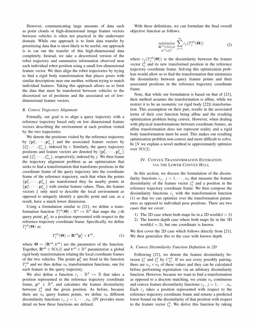
Fig. 4: The feature space for a sample simulated trial is shownin (a). The reference and query trajectories are then generatedas shown in (b) and (c). To simulate the fact that the relativetransformation between trajectories is unknown, we then randomlyrotate and translate the query trajectory and use the proposedand evaluated methods to estimate the inverse of the randomtransformation. The resulting trajectories are shown in (d).

where the inequality constraints and xp and xq are chosenaccording to the specific sub-problem.

Enumerating the possible combinations of these con-straints results in eight sub-problems. Solving all eight sub-problems and then selecting the solution with lowest costenables us to estimate a transformation to align the two tra-jectories without an initial estimate of alignment. In addition,this method enables us to avoid performing data associationand thus perform alignment based on relatively indistinct,low-dimensional, feature observations. We then iterate overthis process with consecutively smaller regions of interest,as explained in Section 4 of [21], to decrease the number ofreference trajectory points used to create the cost functionand thus increase accuracy.

B. Parallel and Feature Agnostic Implementation

We implemented the proposed system in c++. The releasedimplementation uses MOSEK [27] and multiple threads toefficiently solve the linear sub-problems in parallel. Thereleased code can be found at the following link:https://bitbucket.org/jmangelson/cte.

Our implementation and method are agnostic to the under-lying feature space. When specifying a problem to be solved,the user provides feature point positions and a function thatcalculates the feature dissimilarity of a given pair of points.As such, the specifics of the feature space being used andthe dissimilarity function are free to be chosen by the user.

In addition to our own proposed method for approximateoptimization over SO(2), we also implemented functionalityfor estimating affine and symmetric transformations [21], aswell as rigid body transformations via conv SO(2) [19] forcomparison.

TABLE I: Comparison of the proposed linear programmingbased method with other convex transformation estimation algo-rithms. Standard deviation shown is after removing outliers outside1.5*IQR, IQR=Inter-Quartile-Range.

Proposed SOConvHull [19] Symmetric [21] Affine [21]Rotation Median SE 0.011 0.039 0.042 0.338Rotation Stddev SE 0.017 0.096 0.095 0.498Trans. Median SE (m2) 4.796 10.974 11.601 32.582Trans. Stddev SE (m2) 6.770 18.219 20.318 57.370% Approx. Valid Rotations 100.0 37.0 25.5 1.0Avg Runtime (s) 41.444 29.527 25.416 23.926

VII. COMPARISON WITH EXISTING CONVEXOPTIMIZATION METHODS

To provide quantitative results, we generated 200 syntheticworlds with smoothly varying feature spaces. We then sim-ulated both a reference and a query lawn-mower trajectorywithin that space and randomly rotated and translated thequery trajectory. Finally, we compared the alignment resultsfrom a variety of convex alignment methods formulated asin §IV but with different types of transformation constraints.Specifically, we compared our proposed linear programming-based approach to methods based on [21] that allowed eitheraffine or symmetric transformations as well as a methodthat enforced that the estimated transformation lie within theconvex hull of SO(2) [19]. Fig. 4 shows a sample simulatedtrajectory and associated alignment results. The nominaltrackline width for this dataset was two meters and thefeature vector dimension was three.

Table I provides a summary of the comparison results. Ourproposed method outperforms other methods in all metricsexcept for runtime. Note that the median translation squarederror for the proposed method is 4.796 meters squared whilethe resolution of the tracklines simulated was two meters,meaning that the median error is only slightly higher thanthe resolution of the input data.

The current implementation uses four threads that indepen-dently solve two linear programs each via the optimizationlibrary Mosek [27]. However, the speed of the algorithm canbe additionally improved by increasing the number of coresor by using a faster convex optimization library.

VIII. APPLICATION TO MULTI-AGENT AUTONOMOUSSHIP HULL INSPECTION

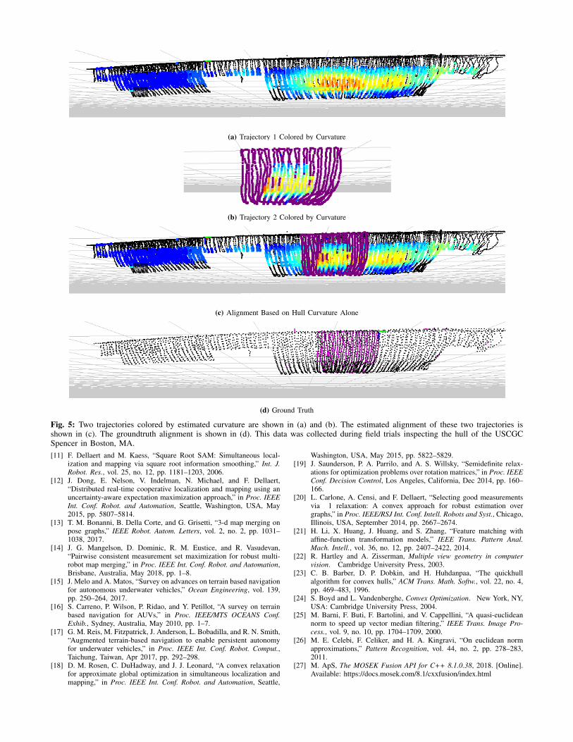
We also tested this method on real-world field data col-lected using a Hovering Autonomous Underwater Vehicle(HAUV) performing autonomous ship hull inspection. Weused the sparse range returns of the Doppler velocity log(DVL) to estimate the curvature of the hull. Then, by treatingthe local curvature of the ship hull as a feature vector, weare able to re-localize to an earlier trajectory using only theDVL. Fig. 5 shows an alignment using this method.

Using the proposed alignment method limits the infor-mation that needs to be passed between vehicles to sixfixed or floating-point values for each position visited bythe agent (including three position coordinates and threecurvature feature values), while the throughput needed totransfer image features between agents would be on the orderof 1000-10000 fixed or floating-point values per position.

Thus, the proposed method results in a decrease in requiredthroughput of approximately 3-4 orders of magnitude.

The final accuracy of the alignment is dependent on thedistinctiveness of the features being observed as well as thesampling resolution inherited from the reference trajectory.However, as formulated, the proposed method is independentof the specific feature and thus can be applied to whateverfeature set is most distinctive in a given environment, sub-ject to the communication bandwidth available. In addition,alignment can be further refined if desired using higherdimensional data such as imagery once an initial estimateof alignment has been obtained, thus minimizing the amountof image data that must be transferred between agents.

IX. CONCLUSION

In this paper, we propose a method for aligning robot tra-jectories that is linear and thus does not require initialization.In addition, the proposed method aligns trajectories withoutperforming data association which decreases the amount ofinformation that must be transferred between agents. Wecompared the existing method to similar convex methods thatfail to enforce that the estimated transformation be rigid. Wealso applied the proposed algorithm to localization in thecontext of multi-agent autonomous ship hull inspection.

Future work would include: extending the proposed ideasto three dimensions and relaxing the assumption that thequery trajectory be contained within the convex hull of thereference trajectory.

REFERENCES[1] F. S. Hover, R. M. Eustice, A. Kim, B. Englot, H. Johannsson,

M. Kaess, and J. J. Leonard, “Advanced perception, navigation andplanning for autonomous in-water ship hull inspection,” Int. J. Robot.Res., vol. 31, no. 12, pp. 1445–1464, 2012.

[2] J. M. Walls, A. G. Cunningham, and R. M. Eustice, “Cooperativelocalization by factor composition over a faulty low-bandwidth com-munication channel,” in Proc. IEEE Int. Conf. Robot. and Automation,Seattle, WA, USA, May 2015, pp. 401–408.

[3] V. Indelman, E. Nelson, J. Dong, N. Michael, and F. Dellaert,“Incremental distributed inference from arbitrary poses and unknowndata association: Using collaborating robots to establish a commonreference,” IEEE Control Syst. Mag., vol. 36, no. 2, pp. 41–74, 2016.

[4] L. Carlone, M. K. Ng, J. Du, B. Bona, and M. Indri, “Rao-blackwellized particle filters multi robot SLAM with unknown initialcorrespondences and limited communication,” in Proc. IEEE Int. Conf.Robot. and Automation, Anchorage, Alaska, USA, May 2010, pp. 243–249.

[5] A. Howard, M. J. Matark, and G. S. Sukhatme, “Localization formobile robot teams using maximum likelihood estimation,” in Proc.IEEE/RSJ Int. Conf. Intell. Robots and Syst., vol. 1. Lausanne,Switzerland: IEEE, Oct 2002, pp. 434–439.

[6] X. S. Zhou and S. I. Roumeliotis, “Multi-robot slam with unknowninitial correspondence: The robot rendezvous case,” in Proc. IEEE/RSJInt. Conf. Intell. Robots and Syst. Beijing, China: IEEE, Oct 2006.

[7] L. A. Andersson and J. Nygards, “C-sam: Multi-robot slam usingsquare root information smoothing,” in Proc. IEEE Int. Conf. Robot.and Automation, Pasadena, CA, USA, May 2008, pp. 2798–2805.

[8] B. Kim, M. Kaess, L. Fletcher, J. Leonard, A. Bachrach, N. Roy, andS. Teller, “Multiple relative pose graphs for robust cooperative map-ping,” in Proc. IEEE Int. Conf. Robot. and Automation, Anchorage,Alaska, USA, May 2010, pp. 3185–3192.

[9] A. Cunningham, K. M. Wurm, W. Burgard, and F. Dellaert, “Fullydistributed scalable smoothing and mapping with robust multi-robotdata association,” in Proc. IEEE Int. Conf. Robot. and Automation, St.Paul, Minnesota, USA, May 2012, pp. 1093–1100.

[10] R. M. Eustice, H. Singh, and J. J. Leonard, “Exactly sparse delayed-state filters for view-based slam,” IEEE Trans. on Robotics, vol. 22,no. 6, pp. 1100–1114, 2006.

(a) Trajectory 1 Colored by Curvature

(b) Trajectory 2 Colored by Curvature

(c) Alignment Based on Hull Curvature Alone

(d) Ground Truth

Fig. 5: Two trajectories colored by estimated curvature are shown in (a) and (b). The estimated alignment of these two trajectories isshown in (c). The groundtruth alignment is shown in (d). This data was collected during field trials inspecting the hull of the USCGCSpencer in Boston, MA.[11] F. Dellaert and M. Kaess, “Square Root SAM: Simultaneous local-

ization and mapping via square root information smoothing,” Int. J.Robot. Res., vol. 25, no. 12, pp. 1181–1203, 2006.

[12] J. Dong, E. Nelson, V. Indelman, N. Michael, and F. Dellaert,“Distributed real-time cooperative localization and mapping using anuncertainty-aware expectation maximization approach,” in Proc. IEEEInt. Conf. Robot. and Automation, Seattle, Washington, USA, May2015, pp. 5807–5814.

[13] T. M. Bonanni, B. Della Corte, and G. Grisetti, “3-d map merging onpose graphs,” IEEE Robot. Autom. Letters, vol. 2, no. 2, pp. 1031–1038, 2017.

[14] J. G. Mangelson, D. Dominic, R. M. Eustice, and R. Vasudevan,“Pairwise consistent measurement set maximization for robust multi-robot map merging,” in Proc. IEEE Int. Conf. Robot. and Automation,Brisbane, Australia, May 2018, pp. 1–8.

[15] J. Melo and A. Matos, “Survey on advances on terrain based navigationfor autonomous underwater vehicles,” Ocean Engineering, vol. 139,pp. 250–264, 2017.

[16] S. Carreno, P. Wilson, P. Ridao, and Y. Petillot, “A survey on terrainbased navigation for AUVs,” in Proc. IEEE/MTS OCEANS Conf.Exhib., Sydney, Australia, May 2010, pp. 1–7.

[17] G. M. Reis, M. Fitzpatrick, J. Anderson, L. Bobadilla, and R. N. Smith,“Augmented terrain-based navigation to enable persistent autonomyfor underwater vehicles,” in Proc. IEEE Int. Conf. Robot. Comput.,Taichung, Taiwan, Apr 2017, pp. 292–298.

[18] D. M. Rosen, C. DuHadway, and J. J. Leonard, “A convex relaxationfor approximate global optimization in simultaneous localization andmapping,” in Proc. IEEE Int. Conf. Robot. and Automation, Seattle,

Washington, USA, May 2015, pp. 5822–5829.[19] J. Saunderson, P. A. Parrilo, and A. S. Willsky, “Semidefinite relax-

ations for optimization problems over rotation matrices,” in Proc. IEEEConf. Decision Control, Los Angeles, California, Dec 2014, pp. 160–166.

[20] L. Carlone, A. Censi, and F. Dellaert, “Selecting good measurementsvia 1 relaxation: A convex approach for robust estimation overgraphs,” in Proc. IEEE/RSJ Int. Conf. Intell. Robots and Syst., Chicago,Illinois, USA, September 2014, pp. 2667–2674.

[21] H. Li, X. Huang, J. Huang, and S. Zhang, “Feature matching withaffine-function transformation models,” IEEE Trans. Pattern Anal.Mach. Intell., vol. 36, no. 12, pp. 2407–2422, 2014.

[22] R. Hartley and A. Zisserman, Multiple view geometry in computervision. Cambridge University Press, 2003.

[23] C. B. Barber, D. P. Dobkin, and H. Huhdanpaa, “The quickhullalgorithm for convex hulls,” ACM Trans. Math. Softw., vol. 22, no. 4,pp. 469–483, 1996.

[24] S. Boyd and L. Vandenberghe, Convex Optimization. New York, NY,USA: Cambridge University Press, 2004.

[25] M. Barni, F. Buti, F. Bartolini, and V. Cappellini, “A quasi-euclideannorm to speed up vector median filtering,” IEEE Trans. Image Pro-cess., vol. 9, no. 10, pp. 1704–1709, 2000.

[26] M. E. Celebi, F. Celiker, and H. A. Kingravi, “On euclidean normapproximations,” Pattern Recognition, vol. 44, no. 2, pp. 278–283,2011.

[27] M. ApS, The MOSEK Fusion API for C++ 8.1.0.38, 2018. [Online].Available: https://docs.mosek.com/8.1/cxxfusion/index.html