Embed Size (px)
Citation preview

JOIMwww.joim.com
Journal Of Investment Management, Vol. 16, No. 2, (2018), pp. 17–46
© JOIM 2018
COMMON FACTORS IN CORPORATE BOND RETURNSRonen Israela,c, Diogo Palharesa,d and Scott Richardsonb,e
We find that four well-known characteristics (carry, defensive, momentum, and value)explain a significant portion of the cross-sectional variation in corporate bond excessreturns. These characteristics have positive risk-adjusted expected returns and are notsubsumed by traditional market premia or respective equity anomalies. The returns areeconomically significant, not explained by macroeconomic exposures, and there is someevidence that mispricing plays a role, especially for momentum.
1 Introduction
Corporate bonds are an enormous—and grow-ing—source of financing for companies aroundthe world. As of the first quarter of 2016, therewas $8.36 trillion of U.S. corporate debt out-standing, and from 1996 to 2015 corporate bondissuance grew from $343 billion to $1.49 trillion(Securities Industry and Financial Markets Asso-ciation). Surprisingly little research, however, hasinvestigated the cross-sectional determinants ofcorporate bond returns.
We study the drivers of the cross-section of cor-porate bond expected returns. To do so, we focuson a set of characteristics that has been shown to
aAQR Capital Management, Greenwich, CT.bAQR Capital Management, London Business School,London, United Kingdom.cE-mail: [email protected]: [email protected]: [email protected]
predict returns in other markets, yet researchershave not studied the viability of all these charac-teristics to predict returns in credit markets. Thecharacteristics are carry, quality, momentum, andvalue (Koijen et al., 2014 for carry; Frazzini andPedersen, 2014 for quality; Asness et al., 2013 formomentum and value). Our contribution includes(i) applying these concepts to credit markets; (ii)studying them together in a way that shines lighton their joint relevance or lack thereof; (iii) eval-uating their economic significance by examiningboth long-and-short, transaction-costs-obliviousportfolios, and also long-only, transaction-costsaware portfolios; and (iv) exploring the sourceof the return premia by testing both risk- andmispricing explanations.
Using traditional long-and-short portfolio analy-sis and cross-sectional regressions we find pos-itive risk premiums that are highly significant(t-statistics of 3 or more) for all characteristics
Second Quarter 2018 17

18 Ronen Israel et al.
but carry. These premia are distinct from tra-ditional long-only bond and equity market riskpremia, as well as from the premium earned bylong-and-short equity anomalies based on value,momentum and defensive. The strong relationamong carry, defensive, value and momentumand future credit excess returns can be interpretedas out-of-sample evidence for the broader efficacyof these characteristics.
We also make a methodological contribution tolong-and-short portfolio analysis for credit mar-kets. The volatility and market beta of corporatebonds is tightly related to credit spreads anddurations. Many return predictors are also cor-related with credit spreads. As a consequence,if one just creates portfolios by sorting on thesemeasures, the long-and-short portfolios will havevery different risk profiles, making their expectedreturns hard to compare and the long-high-short-low portfolio far from market neutral. In the end,contrary to what happens in equity long-and-short portfolios that end up with small marketexposures, simple long-and-short credit portfo-lios do not. Furthermore, credit spread itself is areturn predictor so it is important to understandwhether a candidate variable simply predictsreturns because of its correlation with spreads orwhether it has any extra forecasting power. Tosolve these general issues, we use a double sort onan ex-ante measure of beta (duration times spread)and the candidate characteristic.
Trading costs and liquidity are also very differ-ent in credit markets relative to equity markets.Corporate bonds are difficult to trade and theexpected trading cost is high relative to the under-lying volatility of the asset class (see, e.g., Harris,2015). Thus, simple analyses of Sharpe ratiosbased on “academic” quintile long/short port-folios may substantially overstate the economicsignificance of any characteristic. Thus, whenstudying credit portfolios, we explicitly account
for transaction costs and other potential tradingrestrictions.
To establish more realistic returns we also studylong-only portfolios of relatively liquid corpo-rate bonds with exposure to carry, defensive,momentum and value themes. We show that theseportfolios generate high risk-adjusted returns, netof trading costs. Relative to a value-weightedbenchmark of corporate bonds, the long-onlyportfolio yields a net (of transaction cost) activereturn of 2.20% annualized, which translates toan information ratio of 0.86. While the number isa point estimate out of a roughly 20-year sample,its exact magnitude is less important than the factthat it is well above zero.
We explore possible explanations for theobserved return’s patterns. We examine both riskexplanations–characteristic portfolios expose theaggregate investor to losses at times in whichthose losses are particularly tough to bear–andmispricing theories–investors deviate from ratio-nality because of mistakes or agency problemsand limits-to-arbitrage stop arbitrageurs fromfully correcting these mistakes and their impacton asset prices.
We examine the risk hypothesis with two tests.First we measure the exposure of each indi-vidual characteristic and a combination of allof them to traditional macroeconomic factors(e.g., Chen et al., 1986). While the coefficientsare statistically significant, they suggest that thecharacteristics have a hedging profile. That is,the returns of the combined portfolio are higherwhen growth expectations are lower, volatilityincreases and inflation expectations increase. Inthe second test, we replace the traditional macroe-conomic factors with changes in broker–dealerleverage. Adrian et al. (2014) found that expo-sures to broker–dealer balance sheets can explainequity anomalies as well as government bond
Journal Of Investment Management Second Quarter 2018

Common Factors in Corporate Bond Returns 19
returns. We do not find evidence that broker–dealer leverage can explain credit characteristicreturns. In particular, the combined portfolio,exposed to all individual characteristics, has apositive (hedging), but indistinguishable fromzero, loading on leverage shocks.
We break down the drivers of mispricing into(i) factors that influence the likelihood that noisetraders (Grossman and Stiglitz, 1980) are impor-tant for a given security; and (ii) factors that limitthe activity of arbitrageurs (Shleifer and Vishny,1997). We proxy for the likelihood of noise traderswith (i) a measure of the investor base sophistica-tion (institutional ownership of the bond); and (ii)a measure of firm transparency (analyst coverageof the issuing firm equity). For limits to arbitragewe measure liquidity (bond amount outstanding)and ease of shorting (as reflected by the shortingfee).
We run two tests using with those proxies. Inthe first test we examine whether the bonds mostattractive to an arbitrageur–those with extremevalues for the anomalies–are particularly hardto arbitrage or are more vulnerable to investor’serrors. For the shorting fee the test is one sided:are bonds that represent the most attractive shortfrom the point of view of arbitrageurs–those withunusually low anomaly scores–unusually hard toshort? We do not find evidence of this pattern forany of the characteristics.
In the second test we look at long-and-short port-folios built on security universes which differ inexpected mispricing and limits to arbitrage. Thehypothesis here is that anomaly returns shouldbe stronger among the hard-to-arbitrage-or-high-error bonds. Momentum returns are indeed largeramong harder-to-arbitrage-or-high-error bondsand the result is statistically significant. The otheranomalies perform similarly across the differentuniverses.
Finally, the last test focuses on the investor mis-take hypothesis. We test whether the returns canbe explained by investors’ errors in forecastingsales (e.g., Bradshaw et al., 2001). To proxy forinvestors’ expectations, which are unobservable,we use equity analyst forecasts. If these forecastswere rational and unfettered by agency conflicts,analyst revisions should not be predictable bypublic information. On the other hand, if theyunderestimate the sales of firms with high scoresand overestimate the sales of those with lowscores, the correction of those expectations mayexplain the anomaly premium. The evidence isin the right direction, statistically significant andquantitatively important for momentum, but notfor the remaining characteristics. Overall, returnsto the momentum characteristic seem to be themost tightly linked to mispricing, with the evi-dence being less clear about the source of thereturns of other characteristics.
The remainder of this paper proceeds as fol-lows. Section 2 discusses a simple frameworkfor corporate bond excess returns and links ouranalysis to earlier papers exploring determinantsof cross-sectional variation in corporate bondexpected excess returns. Section 3 explains ourdata sources, sample-selection criteria, charac-teristic measures and research design. Section 4describes our empirical analyses and Section 5concludes.
2 A framework for expected corporate bondexcess returns
Unlike equity markets with variants of the divi-dend discount model to guide empiricists in theirmeasurement of expected returns, there is notan agreed upon framework for estimating excesscredit returns. Ex post, researchers agree thatcredit excess returns can, and should, be mea-sured as the difference between the returns to acorporate bond and an appropriately cash flow-matched treasury bond (see, e.g., Hallerbach
Second Quarter 2018 Journal Of Investment Management

20 Ronen Israel et al.
and Houweling, 2013; Asvanunt and Richardson,2017). Ex ante, as credit and equity are relatedsecurities, one approach would be to simplyexplore whether characteristics known to explaincross-sectional variation in equity excess returnsalso explain credit excess returns. Indeed, somerecent research has followed this approach (e.g.,Chordia et al., 2016). This approach amountsto testing whether priced sources of risk spanacross markets (e.g., Fama and French, 1993).Whilst this approach is useful in commentingon whether characteristics share similar returnsacross equity and credit markets, this approachmisses an important point that the relevant riskacross credit and equity markets are not identi-cal. After all, simply documenting that: (i) X iscorrelated with equity excess returns, (ii) equityexcess returns and credit excess returns are cor-related, and hence (iii) X is therefore correlatedwith credit excess returns is not that exciting (seee.g., Lok and Richardson, 2011).
Prices of corporate bonds are not independentfrom equity prices, but nor are they simply a mir-ror image. First, while the fundamental value ofbonds and equities both depend on the underlyingvalue of the assets of the firm (e.g., Merton, 1974),the way these two assets respond to changes inproperties of asset values is not identical. Sec-ond, equity and bond values can change evenwhen the underlying value of the firm businessdoes not. Corporate events such as leveragedbuyouts, for example, tend to benefit sharehold-ers at the expense of debtholders. Third, bondsand equities are traded in two different marketsand typically held by different investors. Thiscan make stock and bond valuations diverge, asthey are anchored to the risk aversion, liquid-ity demands and sentiment of different investorclienteles. As a consequence, knowledge aboutthe cross-section of expected stock returns doesnot translate one-to-one to bond returns (see, e.g.,Chordia et al., 2016; Choi and Kim, 2015).
Our approach is to directly measure characteris-tics that could inform about expected credit excessreturns. A natural candidate is the spread of thecorporate bond, which we call ‘carry’. This is asuitable measure of expected returns if, and onlyif, there is no change in either default expecta-tions or aggregate risk premium. To complementa measure of spread, we also look to multiplecharacteristics that could potentially inform aboutfuture changes in spreads. Such measures includedimensions of value, momentum and quality thathave been examined in equity markets. But weneed to tailor these measures to reflect the type ofrisk priced in the credit market (notably the riskof default). As such, our paper is related to priorresearch exploring cross-sectional determinantsof corporate bond excess returns.
Correia et al. (2012) study value investing incorporate bond markets by comparing marketspreads with model-implied spreads estimatedusing fundamental and market-based inputs.Kwan (1996) and Gebhardt et al. (2005b) doc-ument strong evidence for equity momentum incorporate bond markets by showing that pastequity returns strongly predict future corporatebond returns of the same issuer, even after con-trolling for corporate bond momentum. Jostovaet al. (2013) examine credit momentum and showthat it is profitable when used to trade high-yieldU.S. corporate bonds—even when controlling forequity momentum.
Koijen et al. (2014) evaluate carry factors acrossseveral markets: for credit markets, they test cor-porate bond indices of varying durations, maturi-ties and rating categories. Carvalho et al. (2014)identify a low-risk anomaly across a broad uni-verse of fixed income assets for various measuresof risk. Similarly, Frazzini and Pedersen (2014)document positive risk-adjusted returns for port-folios that take long positions for short durationand higher-rated corporate bonds and take short
Journal Of Investment Management Second Quarter 2018

Common Factors in Corporate Bond Returns 21
positions for long duration and lower-rated cor-porate bonds. In contrast, Ng and Phelps (2014)note that the low-risk anomaly in corporate bondsis sensitive to the selected measure of risk.
Our work extends this literature. First, we studythe stand-alone performance of characteristicsand investigate the relation between them andtheir combined efficacy. Second, we considersimple unconstrained long–short portfolios andalso more realistically investable long-only port-folios, which account for transaction costs andshorting constraints typical for corporate bonds.The investable portfolios show that our results areeconomically meaningful. Third, we investigatethe sources of return predictability. We explorerisk-based and non-risk-based explanations andfind that macroeconomic exposures are not con-sistent with a positive premia for the anomalies,whereas limits to arbitrage and investor errorsseem to play a role in momentum strategies,though not the others.
3 Data and methodology
3.1 Corporate bond data
Our analysis is based on a comprehensive panelof U.S. corporate bonds between January 1997and April 2015 measured at a monthly fre-quency. This panel includes all constituents ofthe Bank of America Merrill Lynch (“BAML”)investment-grade (“U.S. Corporate Master”) andhigh-yield (“U.S. High Yield Master”) corporatebond indices. The BAML dataset relies on theindustry standard for valuations, aggregating datafrom TRACE as well as other sources. For an aca-demic use of the data see Schaefer and Strebulaev(2008).
Following the criteria of Haesen et al. (2013), weselect a representative bond for each issuer everymonth. The criteria used for identifying the repre-sentative bond are selected so as to create a sample
of liquid and cross-sectionally comparable bonds.Specifically, we select representative bonds on thebasis of (i) seniority, (ii) maturity, (iii) age and (iv)size.
First, we filter bonds on the basis of seniority,limiting ourselves to only senior debt. We thenselect only the bonds corresponding to the mostprevalent rating of the issuer. To do this, we firstcompute the amount of bonds outstanding foreach rating category for a given issuer. We keeponly those bonds that belong to the rating categorythat contains the largest fraction of debt outstand-ing. This category of bonds tends to have the samerating as the issuer. Second, we filter bonds on thebasis of maturity. If the issuer has bonds with timeto maturity between 5 and 15 years, we removeall other bonds for that issuer from the sample. Ifnot, we keep all bonds in the sample. Third, wefilter bonds on the basis of time since issuance. Ifthe issuer has any bonds that are at most 2 yearsold, we remove all other bonds for that issuer. Ifnot, we keep all bonds from that issuer in the sam-ple. Finally, we filter on the basis of size. Of theremaining bonds, we pick the one with the largestamount outstanding. A deliberate consequence ofour bond selection criteria is that we will not beexploring a liquidity premium (such as issue size)for our primary empirical analyses.
Our resulting sample includes 274,665 uniquebond-month observations, corresponding to11,804 bonds issued by 4,296 unique firms.Table 1 reports annual statistics describing thecomposition of our sample over time. The aver-age month in the sample consists of 1,247 bondsrepresenting $573 billion of total notional out-standing, of which 59% (41%) corresponds toinvestment grade (high yield) issues. To constructvariables requiring financial statement informa-tion, we can link 48% of our universe to theCompustat database (using CUSIP and Tickeridentifiers contained in the BAML dataset).
Second Quarter 2018 Journal Of Investment Management

22 Ronen Israel et al.
Table 1 Universe statistics (January 1997–April 2015).
Year Count Total %IG %HY % Linked tonotional Compustat
1997 1,096 239 60% 40% 54%1998 1,188 278 61% 39% 53%1999 1,104 306 63% 37% 52%2000 1,026 335 65% 35% 50%2001 1,026 375 70% 30% 49%2002 1,099 443 70% 30% 49%2003 1,263 511 63% 37% 49%2004 1,398 562 60% 40% 47%2005 1,291 569 59% 41% 45%2006 1,268 560 58% 42% 43%2007 1,256 578 56% 44% 43%2008 1,046 553 64% 36% 47%2009 967 540 66% 34% 49%2010 1,269 689 56% 44% 46%2011 1,380 768 53% 47% 46%2012 1,406 812 53% 47% 46%2013 1,521 893 51% 49% 45%2014 1,564 936 50% 50% 45%2015 1,533 948 51% 49% 46%
Average 1,247 573 59% 41% 48%
The table reports annual summary statistics of the Bank of America Mer-rill Lynch (BAML) bond sample. Each column statistic is computedmonthly and averaged within the specified year. Investment grade (IG)and high yield (HY) classifications are based on S&P ratings. Bond issuesare linked to Compustat based on CUSIPs and Tickers as described inthe text. Total notional is reported in billions of dollars.
Next, we describe a few key variables containedin the BAML dataset. Option-adjusted spread(OAS) is the fixed spread that needs to be addedto the Treasury curve such that the corporatebond’s discounted payments match to its tradedmarket price (accounting for embedded options).Duration, which measures a bond’s sensitivityto interest rates, is also adjusted for embeddedoptionality. BAML provides total returns as wellas excess returns, which are equal to total returnsminus the return of a duration-matched Treasury.Credit ratings are based on Standard & Poor’s rat-ings classification system. To construct numerical
ratings that can be used in our regressions, wemap ratings of AAA, AA, A, BBB, BB, B, CCC,CC, C and D to scores of 1, 2, 3, 4, 5, 6, 7, 8, 9and 10, respectively. Arating less (greater) than orequal to 4 (5) therefore corresponds to investmentgrade (high yield). As newly issued bonds tendto be more liquid, we define a measure of bondilliquidity labelled “age percent,” which is com-puted as time-since-issuance (in days) divided byoriginal maturity (in days).
Table 2 provides a description of several issueand issuer characteristics. All of our variable
Journal Of Investment Management Second Quarter 2018

Common Factors in Corporate Bond Returns 23
Table 2 Issue and issuer characteristics (January 1997–April 2015).
Mean Std. 5% 10% 25% 50% 75% 90% 95%
OAS 386 308 85 107 161 302 512 783 1,002Duration 5.1 2.2 1.6 2.4 3.8 5.0 6.3 7.3 8.2Total Ret. 0.6% 3.1% −2.9% −1.6% −0.4% 0.6% 1.7% 3.0% 4.2%Excess Ret. 0.2% 3.0% −3.2% −1.9% −0.7% 0.2% 1.2% 2.4% 3.6%Amt. Out. 437 442 134 159 208 309 495 811 1,123Time to Mat. 7.8 5.1 2.7 3.9 5.5 7.1 8.7 10.4 15.5Age Percent 28% 19% 5% 7% 12% 24% 39% 54% 67%Rating 4.7 1.4 2.5 3.0 3.8 4.7 6.0 6.6 6.9Dist. to Def 6.0 3.5 1.4 2.0 3.4 5.5 8.0 10.6 12.2Momentum 5% 16% −16% −10% −3% 2% 11% 24% 36%Leverage 0.31 0.41 −0.02 0.03 0.13 0.28 0.47 0.66 0.77
The table reports summary statistics of bond issue and issuer characteristics (as defined in Table A.I). For eachcharacteristic, the column statistic is computed on a monthly basis and then averaged over the full sample period.
definitions are presented in Table A.1. For eachcharacteristic, we compute several statistics (e.g.,mean, standard deviation and various percentiles)on a monthly basis and report the average of thesemonthly statistics in the table. The average issuein our sample has an OAS of 386 basis points,duration of 5.1 years, $437 million of notionaloutstanding, 7.8 years to maturity, and age per-cent of 28%. The average issuer in our samplehas a six-month average credit and equity excessreturn of 5% and market leverage of 0.31.
3.2 Characteristic measures
In this section, we define the four key charac-teristics that we use to explain cross-sectionalvariation in corporate bond excess returns. Ourchoices are driven by the desire to have intuitiveand, to the extent possible, standard measuresthat span both public and private issuers of cor-porate bonds. When multiple measures satisfythose criteria, we combine them using equal-riskweights to obtain a more robust portfolio andmake the results less susceptible to a specific vari-able selection.1 We deliberately do not select sizeas a characteristic, as the corporate bond market
is notoriously expensive to trade. Our interest isin the identification of characteristics that explainexcess returns of large and liquid corporate bonds.
Carry is the return of a security if time passesbut market conditions do not change and we mea-sure it using the option-adjusted spread (OAS).We use OAS rather than bond yield because we areinterested in credit returns in excess of key-rate-duration-matched treasuries. Bond yield reflectsboth the credit component and the Treasurycomponent.
OAS also has its problems. It is a perfect mea-sure of carry only if the credit curve is flat. Ifthe curve has a positive or negative slope, OASwill underestimate and overestimate carry respec-tively. Most issuers have upward sloping creditspread term structures, implying that the OAS willbe an imperfect measure of carry. The alternative,however, is to estimate credit spread curves foreach issuer. While potentially more precise, thecurve interpolation exercise is model dependentand adds considerable complexity and opaque-ness to the carry measure. In our view, OASstrikes a reasonable balance between precision on
Second Quarter 2018 Journal Of Investment Management

24 Ronen Israel et al.
one hand and simplicity and transparency on theother.
Past research has identified a tendency for saferlow-risk assets to deliver a higher risk-adjustedreturn (e.g., Frazzini and Pedersen, 2014; Car-valho et al., 2014). We apply this idea to corporatebonds by building a defensive (or low-risk) mea-sure using multiple variables. Our first measureis market leverage, measured as the value of netdebt (book debt + minority interest + preferredstocks − cash) divided by the sum of the valueof net debt and market value of equity. Bothintuitively and theoretically speaking, firms withhigher levels of leverage (or greater use of debt)are more likely to default and are hence funda-mentally riskier (e.g., Altman, 1968; Shumway,2001).
Our second measure of safety is gross profitabil-ity as defined in Novy–Marx (2013). Unlike otherprofitability measures, such as net income overequity value, gross profitability speaks to the qual-ity of the overall assets owned by the firm. Assuch, it reasonably proxies for the safety of theenterprise, covering both equity and debt claims.
Our third measure of safety is simply low dura-tion. Binsbergen and Koijen (2015) documentthat short maturity securities across different assetclasses tend to have higher risk-adjusted returns.Palhares (2013) has shown that this also holdsamong single-name credit default swaps. Here weapply the same concept to corporate cash bonds.
For financial instruments that trade in cash mar-kets (i.e., government bonds and equities), thereis reliable evidence of a negative relation betweenbeta and future excess returns (e.g., Frazziniand Pedersen, 2014). One reason for this nega-tive relation is the prevalence of leverage-averseinvestors in cash markets who seek higher returnsby buying higher beta assets as opposed to lev-ering up the mean–variant efficient portfolio.
Indeed, evidence from holdings of equity mutualfunds shows that the average stock held has abeta of about 1.08 (see Table 11 of Frazzini andPedersen, 2014).
For credit markets, both systematic and idiosyn-cratic volatility can be captured by the productof duration and spread, or DTS (e.g., Ben Doret al., 2007). The first component, duration, hasbeen shown to be negatively associated with risk-adjusted returns in equities, bonds and severalother asset classes (e.g., Palhares, 2013; Binsber-gen and Koijen, 2015). The second component,credit spread, simply measures carry in creditmarkets. Beta and idiosyncratic volatility, there-fore, implicitly combine two measures that haveconfounding effects on expected returns, leadingto their inadequacy as suitable characteristics toexplain corporate bond excess returns. As a con-sequence we have excluded beta and volatility asmeasures of the defensive theme.
For our momentum characteristic, we use twowidely studied momentum measures. The firstis credit momentum defined as the trailing six-month bond excess return. Jostova et al. (2013)shows that, in a broad sample of corporate bonds,including both high-yield and investment-gradesecurities, past winners tend to outperform pastlosers. The second momentum measure is thesix-month equity momentum of the bond issuer.Kwan (1996) and Gebhardt et al. (2005b) showthat stock returns tend to lead corporate bondreturns.
To construct a value signal, we need a marketvalue measure (price, yield, spread, etc.), a fun-damental value measure and a way to compare thetwo. For example, Fama and French (2003) usethe price of a stock for the market measure, thebook value for the fundamental measure and theratio to make a comparison. For credit markets weuse the spread of the bond and credible measures
Journal Of Investment Management Second Quarter 2018

Common Factors in Corporate Bond Returns 25
of default risk as the fundamental anchor. A cheapbond has high spread relative to default risk.
We use two proxies for default risk. First, wefollow Correia et al. (2012) and use the issuerdefault probability. We measure the default prob-ability as in Bharath and Shumway (2008). Onedrawback of this approach is that it can only becomputed for issuers with publicly traded equity.To increase coverage, we use a second valueanchor that combines three broadly available fun-damental measures: credit rating, bond durationand the volatility of bond excess return returns inthe last 12 months.
3.3 Portfolio construction
The traditional way of examining the relationshipbetween expected returns and a candidate predic-tor in the equity literature consists of constructingportfolios based on the cross-sectional rank of thecharacteristic, averaging the returns within theportfolio and then averaging those over time (e.g.,Fama and French, 1993). This approach doesnot guarantee that the different quantile portfo-lios will have similar ex-ante volatilities and beta,and, as consequence, that the long-top-minus-short-bottom portfolios will be market neutral. Inspite of that, in the equity literature, the differ-ent anomaly portfolios do tend to have similarrisk and the long-and-short risk factors tend tohave moderate betas—though not zero, for exam-ple, the SMB and HML factors are notoriousfor their positive and negative betas respectively(e.g., Fama and French, 1993) and the betting-against-beta factor (e.g., Frazzini and Pedersen,2014) has negative beta.
This quirk of the traditional portfolio constructionmethodology is important for this paper becausethe cross-section of corporate bonds has a muchlarger dispersion in beta and risk than equity mar-kets. Furthermore, many of the characteristic we
examine correlate with beta. As a consequence,the long-and-short portfolios formed using thosecharacteristics will not be beta neutral, complicat-ing the interpretation of their expected returns andtime-series properties as the reflection of some-thing other than their embedded market exposure.To obtain long-and-short portfolios that are closerto market neutrality we demean characteristicswithin five ex-ante beta quintiles, with beta beingmeasured as duration times spread (DTS). Weexclude duration and carry from that step because,mechanically, that would induce a portfolio thatmixes high carry and low duration together.
We construct two types of characteristic portfo-lios. First, we follow the standard convention ofcomputing a zero-cost portfolio, that is, long cor-porate bonds in the highest quintile of a givencharacteristic and short corporate bonds in thelowest quintile of a given characteristic. Withinquintiles, we report excess returns based on value-weighted returns. Our inferences are unaffected ifwe instead use equal weighting. We also display aconstant 5% volatility version of each long-and-short portfolio (Muir and Moreira, 2016). We usethe 24-month realized volatility of the unsealedportfolio as the measure of ex-ante risk.2
We construct the quintiles and long-and-shortportfolios for each characteristic individually andfor a combination of them all. The combinationsorting variable is an inverse-of-risk-weightedsum of the four characteristics. More precisely,for each characteristic we form a portfolio thatis linear in ranks (Asness et al., 2014) and thenmultiply it by 5% and divide it by its 24-monthrealized volatility—the outcome is an alternativeconstant-volatility portfolio with linear weightsinstead of just having non-zero values for themost extreme quintiles. The combined charac-teristic is then just an equal-weighted average ofthose single-characteristic, linear-in-ranks port-folio weights.
Second Quarter 2018 Journal Of Investment Management

26 Ronen Israel et al.
A critical part of this paper is to examine thereturn-forecasting characteristics jointly. Eachsingle characteristic informs us about propertiesof the stochastic discount factor that prices corpo-rate credit securities, but the single portfolio thatmakes optimal use of the multiple characteristicsgoes beyond: it alone is sufficient to fully charac-terize that discount factor (e.g., Cochrane, 2009).From the point of view of an investor, that singleportfolio is also interesting. For example, for amean–variance investor allocating between theselong-and-short credit strategies and cash, the allo-cation to that optimal portfolio would be sufficientto summarize its asset allocation policy.
The question is then how to build this optimalportfolio. Without observing expected returns andcovariance matrices, one cannot observe the opti-mal portfolio weights. Using sample moments isproblematic because of look-ahead bias and therelative shortness of a 20-year sample to esti-mate expected return. Our answer to the problemis an equal-weighted portfolio. It generalizes therobustness of the 1/N portfolio (e.g., DeMiguelet al., 2009) by applying it to similarly riskycharacteristic portfolios rather than underlyingassets.
For the combination of characteristics, we alsoanalyze a second type of portfolio: a long-onlyportfolio that takes into consideration realisticimplementation by solving a linear optimizationproblem. The analysis of a long-only portfolio isunusual when studying cross-sectional return pre-dictability. But given the well-known challengesin shorting corporate bonds (e.g., Asquith et al.,2013) and the significant costs in trading corpo-rate bonds relative to their underlying volatility(e.g., Bessembinder et al., 2006; Edwards et al.,2007), it is important to test whether the char-acteristic’s premia survives difficult but realisticreal-world constraints.
4 Results
4.1 Regression analysis
Before reporting the performance of our portfo-lios, we first report Fama–Macbeth regressions ofmonthly corporate-bond excess returns regressedonto lagged characteristics along with controlvariables. Each month, we run cross-sectionalregressions of the form:
Ri,t+1 = α + β1CARRY i,t + β2DEFi,t
+ β3MOM i,t + β4VALUEi,t
+ γZ + εi,t+1, (1)
where Ri,t+1 denotes the duration-hedged excessreturn of bond i over month t + 1. Each of thefour characteristics is converted to a normalizedvariable. Specifically, for each characteristic, forevery month, we rank issues by their characteris-tic values, subtract the mean rank and then divideby the standard deviation of the ranks. We alsofill missing values with zero, but the results arerobust if we do not. As a result, estimated coeffi-cients may be interpreted as the future one-monthexcess return difference for a one standard devi-ation difference in characteristic ranking. To ruleout the hypothesis that the characteristics predictreturns because they proxy for traditional mea-sures of risk, we include control variables in theregression. The first variable is a market beta,where the market is defined as the credit returnof the cap-weighted portfolio of all bonds in ourdatabase and the beta is computed using a 12-month rolling regression. For robustness, we alsoinclude two other traditional measures of risk incredit markets—rating and duration—as well asa proxy for illiquidity, age percent (e.g. Gebhardtet al., 2005a).
Table 3 reports our Fama–Macbeth regressionestimates for the monthly sample period from Jan-uary 1997 to April 2015. Regression (1) includesjust an intercept and beta, and Regression (2)
Journal Of Investment Management Second Quarter 2018

Common Factors in Corporate Bond Returns 27
Table 3 Fama–Macbeth regressions (January 1997–April 2015).
(1) (2) (3) (4) (5) (6) (7)
Intercept 0.10 −0.02 0.04 −0.01 0.05 −0.10 −0.02[1.5] −[0.2] [0.5] −[0.1] [0.5] −[1.2] −[0.2]
Carry 0.00 0.14[1.0] [2.3]
Defensive 0.15 0.03[5.0] [0.9]
Momentum 0.15 0.22[3.3] [7.1]
Value 0.26 0.30[5.8] [10.7]
Mkt beta 0.05 0.04 0.10 0.04 0.06 0.08 0.14[0.7] [0.6] [1.6] [0.7] [0.9] [1.2] [2.3]
Rating 0.02 −0.03 0.02 0.00 0.03 0.00[0.8] −[1.0] [0.6] [0.1] [1.0] −[0.1]
Duration −0.01 −0.01 0.01 0.00 0.01 0.01−[0.5] −[0.5] [0.8] −[0.4] [1.1] [1.1]
Age percent 0.25 0.23 0.22 0.23 0.14 0.09[2.2] [2.0] [1.9] [2.0] [1.2] [0.9]
Avg. R-squared 0.07 0.10 0.14 0.10 0.11 0.11 0.15Avg. Num. Obs. 723 671 671 671 671 671 671
The table reports Fama–Macbeth regressions of monthly bond excess returns regressed onto normalizedcarry, defensive, momentum and value style measures along with controls for market beta, rating,duration and age percent variables (as defined in Table A.1).
adds our control variables, which reduce the aver-age number of bonds in the cross-section from723 to 671. Regressions (3) through (6) evaluatethe predictive ability of each of our character-istics on a stand-alone basis. Both individuallyand combined, the value and momentum char-acteristics have explanatory power for corporatebond excess returns. The carry characteristic doesnot exhibit a reliable association with future bondexcess returns as a stand-alone variable but it ismarginally significant when controlling for theremaining characteristics. The opposite is truewith defensive: it is highly significant as a stand-alone variable but loses significance when con-trolling for value and momentum. This suggeststhat the defensive theme in credit may be spanned
by the value and momentum themes. This is notsurprising as the value factors we build for creditmake explicit use of fundamental information.Our value measures identify a bond as cheapwhen its spread is wide relative to default prob-abilities. Our measures of default probabilitiesinclude distance to default and rating information.These fundamental anchors incorporate measuresof leverage and expected profitability. As a conse-quence, it is not surprising that they help explainthe defensive premium.
The average R-squared of the Fama–Macbethcross-sectional regressions is 15%, suggestingthat our characteristics collectively explain a non-trivial portion of the cross-sectional variation in
Second Quarter 2018 Journal Of Investment Management
28 Ronen Israel et al.
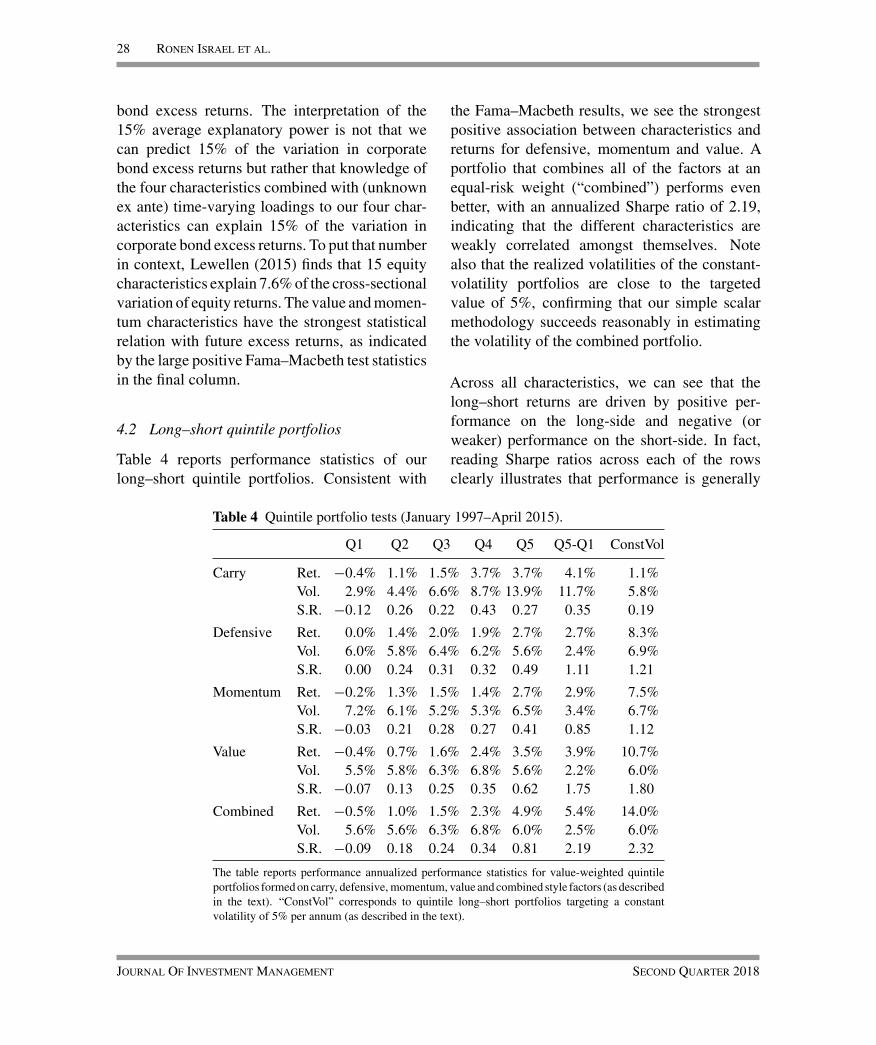
bond excess returns. The interpretation of the15% average explanatory power is not that wecan predict 15% of the variation in corporatebond excess returns but rather that knowledge ofthe four characteristics combined with (unknownex ante) time-varying loadings to our four char-acteristics can explain 15% of the variation incorporate bond excess returns. To put that numberin context, Lewellen (2015) finds that 15 equitycharacteristics explain 7.6% of the cross-sectionalvariation of equity returns. The value and momen-tum characteristics have the strongest statisticalrelation with future excess returns, as indicatedby the large positive Fama–Macbeth test statisticsin the final column.
4.2 Long–short quintile portfolios
Table 4 reports performance statistics of ourlong–short quintile portfolios. Consistent with
the Fama–Macbeth results, we see the strongestpositive association between characteristics andreturns for defensive, momentum and value. Aportfolio that combines all of the factors at anequal-risk weight (“combined”) performs evenbetter, with an annualized Sharpe ratio of 2.19,indicating that the different characteristics areweakly correlated amongst themselves. Notealso that the realized volatilities of the constant-volatility portfolios are close to the targetedvalue of 5%, confirming that our simple scalarmethodology succeeds reasonably in estimatingthe volatility of the combined portfolio.
Across all characteristics, we can see that thelong–short returns are driven by positive per-formance on the long-side and negative (orweaker) performance on the short-side. In fact,reading Sharpe ratios across each of the rowsclearly illustrates that performance is generally
Table 4 Quintile portfolio tests (January 1997–April 2015).
Q1 Q2 Q3 Q4 Q5 Q5-Q1 ConstVol
Carry Ret. −0.4% 1.1% 1.5% 3.7% 3.7% 4.1% 1.1%Vol. 2.9% 4.4% 6.6% 8.7% 13.9% 11.7% 5.8%S.R. −0.12 0.26 0.22 0.43 0.27 0.35 0.19
Defensive Ret. 0.0% 1.4% 2.0% 1.9% 2.7% 2.7% 8.3%Vol. 6.0% 5.8% 6.4% 6.2% 5.6% 2.4% 6.9%S.R. 0.00 0.24 0.31 0.32 0.49 1.11 1.21
Momentum Ret. −0.2% 1.3% 1.5% 1.4% 2.7% 2.9% 7.5%Vol. 7.2% 6.1% 5.2% 5.3% 6.5% 3.4% 6.7%S.R. −0.03 0.21 0.28 0.27 0.41 0.85 1.12
Value Ret. −0.4% 0.7% 1.6% 2.4% 3.5% 3.9% 10.7%Vol. 5.5% 5.8% 6.3% 6.8% 5.6% 2.2% 6.0%S.R. −0.07 0.13 0.25 0.35 0.62 1.75 1.80
Combined Ret. −0.5% 1.0% 1.5% 2.3% 4.9% 5.4% 14.0%Vol. 5.6% 5.6% 6.3% 6.8% 6.0% 2.5% 6.0%S.R. −0.09 0.18 0.24 0.34 0.81 2.19 2.32
The table reports performance annualized performance statistics for value-weighted quintileportfolios formed on carry, defensive, momentum, value and combined style factors (as describedin the text). “ConstVol” corresponds to quintile long–short portfolios targeting a constantvolatility of 5% per annum (as described in the text).
Journal Of Investment Management Second Quarter 2018

Common Factors in Corporate Bond Returns 29
-40%
0%
40%
80%
120%
160%
200%
240%
280%
1997 1999 2001 2003 2005 2007 2009 2011 2013 2015
Carry Defensive Momentum Value Combined
Figure 1 Cumulative style factor returns (January 1997–April 2015).The figure shows cumulative arithmetic returns for each of the carry, defensive, momentum, value and combined style factors (as definedin the text).
monotonically increasing across quintiles foreach of the characteristics.
Figure 1 plots cumulative excess characteristicreturns over time. We can see that performance,especially for the combination of characteristics,is not driven by any particular sub-period and hasnot changed substantially over time. While dif-ferent characteristics performed better and worseover different sub-periods, it is clear that the com-bined portfolio has been relatively stable in itsoutperformance. Not surprisingly the most visibledrawdown is carry during the Global FinancialCrisis, when investors sought safe assets andshunned riskier ones like high-yield bonds (e.g.,Koijen et al., 2014). Whilst we are hesitant todraw too strong inferences from a relatively shorttime period, the relative smoothness of the returnsof the combined portfolio is initial evidence that
risk-based explanations will be challenging tosupport.
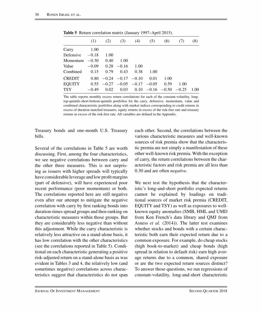
To better understand the source of the characteris-tic’s premia, we report return correlations for thevarious constant-volatility, long-and-short char-acteristic portfolios and well-known sources ofrisk premia. We report the various pairwise returncorrelations in Table 5 using the full time seriesof data for the period January 1997 through toApril 2015, inclusive. We consider the followingtraditional risk premia: (i) credit risk premium(“CREDIT”), measured as the value-weightedcorporate-bond excess returns; (ii) equity risk pre-mium, measured as the difference between thetotal returns on the S&P500 index and one-monthU.S. Treasury bills (“EQUITY”); and (iii) Trea-sury term premium (“TSY”), measured as thedifference between total returns on 10-year U.S.
Second Quarter 2018 Journal Of Investment Management
30 Ronen Israel et al.
Table 5 Return correlation matrix (January 1997–April 2015).
(1) (2) (3) (4) (5) (6) (7) (8)
Carry 1.00Defensive −0.18 1.00Momentum −0.30 0.40 1.00Value −0.09 0.28 −0.16 1.00Combined 0.15 0.79 0.43 0.38 1.00
CREDIT 0.80 −0.24 −0.17 −0.10 0.01 1.00EQUITY 0.55 −0.27 −0.05 −0.17 −0.05 0.59 1.00TSY −0.49 0.02 0.03 0.10 −0.16 −0.50 −0.25 1.00
The table reports monthly excess return correlations for each of the constant-volatility, long-top-quintile-short-bottom-quintile portfolios for the carry, defensive, momentum, value andcombined characteristic portfolios along with market indices corresponding to credit returns inexcess of duration matched treasures, equity returns in excess of the risk-free rate and treasuryreturns in excess of the risk-free rate. All variables are defined in the Appendix.
Treasury bonds and one-month U.S. Treasurybills.
Several of the correlations in Table 5 are worthdiscussing. First, among the four characteristics,we see negative correlations between carry andthe other three measures. This is not surpris-ing as issuers with higher spreads will typicallyhave considerable leverage and low profit margins(part of defensive), will have experienced poorrecent performance (poor momentum) or both.The correlations reported here are still negativeeven after our attempt to mitigate the negativecorrelation with carry by first ranking bonds intoduration-times spread groups and then ranking oncharacteristic measures within those groups. Butthey are considerably less negative than withoutthis adjustment. While the carry characteristic isrelatively less attractive on a stand-alone basis, ithas low correlation with the other characteristics(see the correlations reported in Table 5). Condi-tional on each characteristic generating a positiverisk-adjusted return on a stand-alone basis as wasevident in Tables 3 and 4, the relatively low (andsometimes negative) correlations across charac-teristics suggest that characteristics do not span
each other. Second, the correlations between thevarious characteristic measures and well-knownsources of risk premia show that the characteris-tic premia are not simply a manifestation of theseother well-known risk premia. With the exceptionof carry, the return correlations between the char-acteristic factors and risk premia are all less than0.30 and are often negative.
We next test the hypothesis that the character-istic’s long-and-short portfolio expected returnscannot be explained by loadings on tradi-tional sources of market risk premia (CREDIT,EQUITY and TSY) as well as exposures to well-known equity anomalies (SMB, HML and UMDfrom Ken French’s data library and QMJ fromAsness et al. (2014)). The latter test examineswhether stocks and bonds with a certain charac-teristic both earn their expected return due to acommon exposure. For example, do cheap stocks(high book-to-market) and cheap bonds (highspread in relation to default risk) earn high aver-age returns due to a common, shared exposureor are the two expected return sources distinct?To answer those questions, we run regressions ofconstant-volatility, long-and-short characteristic
Journal Of Investment Management Second Quarter 2018

Common Factors in Corporate Bond Returns 31
portfolio returns on market and equity anomalyreturns as follows:
CONST_VOL_CHARt
= α + β0EQUITY t + β1TSY t + β2CREDIT t
+ β3SMBt + β4HMLt + β5UMDt
+ β6QMJ t + εi,t. (2)
Consistent with the simple correlations reportedin Table 5, we see in Table 6 that the carry char-acteristic has a significant positive exposure tocredit risk premium. After controlling for otherwell-known sources of return, the intercept isnot significant for carry. The defensive charac-teristic is negatively correlated with market riskpremia (e.g. credit risk premium), consistent with
it reflecting a flight to quality or a risk-on/risk-offtendency of investors.
Momentum has a positive correlation with UMDand nothing else. Credit value exhibits a nega-tive loading on SMB and QMJ, −2.0 and −2.3t-statistics, respectively. Interestingly, the valuecharacteristic in credit markets is mildly nega-tively associated with the HML factor, a resultconsistent with the evidence that characteristicportfolios in one asset class have limited corre-lations with those in other asset classes (Asnesset al., 2015). In the fifth column of Table 6,we regress the combined characteristic long–shortportfolio return onto the various market risk pre-mia and equity factor returns. The combinedportfolio does not have a statistically significant
Table 6 Long-and-short portfolioAlphas and Betas with Respect to Marketand Equity Factors (January 1997–April 2015).
Carry Defensive Momentum Value Combined
Intercept 0.05% 0.75% 0.55% 1.02% 1.23%[0.7] [5.3] [3.9] [8.1] [9.6]
CREDIT 0.58 −0.22 −0.19 −0.02 −0.07[10.5] −[2.1] −[1.8] −[0.2] −[0.7]
EQUITY 0.04 −0.07 0.09 −0.11 −0.02[0.0] [0.0] [0.0] [0.0] [0.0]
TSY −0.12 −0.12 −0.10 0.05 −0.18−[2.9] −[1.4] −[1.2] [0.7] −[2.4]
SMB 0.01 0.06 0.01 −0.08 0.02[0.4] [1.3] [0.2] −[2.0] [0.5]
HML −0.02 0.05 0.06 −0.02 0.06−[0.7] [1.2] [1.4] −[0.6] [1.4]
UMD 0.00 −0.01 0.06 −0.01 0.04[0.1] −[0.2] [2.3] −[0.4] [1.6]
QMJ −0.04 0.03 0.11 −0.14 −0.06−[1.2] [0.4] [1.6] −[2.3] −[0.9]
R-squared 0.67 0.10 0.09 0.07 0.05
The table reports monthly excess return regressions of the carry, defensive, momen-tum, value and combined characteristic long-top-quintile-short-bottom-quintile, constant-volatility factors onto (i) market excess returns for treasuries, credit and equity; (ii) equityanomaly factors SMB, HML and UMD from Ken French’s website and QMJ from Asnesset al. (2014). All variables are defined in the Appendix.
Second Quarter 2018 Journal Of Investment Management

32 Ronen Israel et al.
loading on any of the equity factors and a mildlynegative relation with term premium. As a con-sequence, its intercept is a significant 123 basispoints per month with a t-statistic of 9.6 andan information ratio of 2.25. The combinationportfolio is superior to any individual character-istic portfolio reassuring us that the equal-riskapproach is a sensible way to combine the dif-ferent characteristics. Furthermore, the fact thatthe combination portfolio does not load on tradi-tional market risk premia and equity anomaliessuggests that the source of return predictability isdistinct from those.
The economic magnitude of the intercept requiresfurther discussion. The literal interpretationwould suggest that a 2.25 information ratio isavailable for investors. Such a statement needsto be interpreted very cautiously. Corporate bondand equity markets differ substantially in terms oftheir trading costs.
For example, Chen et al. (2007) show that theaverage bid-mid spread for BBB-rated and B-rated medium maturity bonds are 22 bps and30 bps, respectively. Frazzini et al. (2012) reportaverage value-weighted trading costs for globalequities of 20 bps. These numbers, however,severely understate the impact of transactioncosts, as stocks are much more volatile thanbonds. Andersen et al. (2001) find that the medianstock volatility is 22%, whereas the median bondin our sample has an excess return volatilityclose to 7%. More importantly, whereas our com-bined one-dollar-long-and-one-dollar-short port-folio from Table 4 has a 2.5% annualized volatil-ity, Fama–French HML’s factor—long 1 dollarof cheap stocks and short 1 dollar of expensivestocks—achieves 11.6% annual volatility over thesame period.
Given the similarity in dollar transaction costsestimates across bonds and stocks, and similarturnover across bond and stock portfolios, the
bond portfolio transaction cost per unit of riskis more than four times larger than that of equity.As a consequence, if a long-and-short portfolioof stocks and bonds are to have similar net-of-transaction costs Sharpe ratios, the bond portfoliomust have a much larger gross-of-transaction costSharpe ratio.
To illustrate any time-varying performance acrossthe various characteristics (in Figure 2), weuse the full-sample regression coefficients fromTable 6 to compute 36-month rolling aver-age alphas for each respective long-and-short,constant-volatility characteristic portfolio. Whileoutperformance has been marginally attenuatedin recent years, it is clear that excess returnshave been relatively stable and positive. Again thesmoothness of the returns, albeit over a short timeseries, is difficult to reconcile with a risk-basedexplanation. We formally examine this issue inSection 4.4.
4.3 Long-only optimized portfolio
While our long–short characteristic portfoliossuggest a robust relation between credit excessreturns and each of the considered characteris-tics, they do not take into account actual portfolioimplementation considerations. To more realisti-cally address the hypothetical performance of ourcharacteristic portfolios, we build and test opti-mized long-only portfolios with explicit portfolioimplementation constraints. Hence our optimizedportfolios are designed to be comparable withtraditional actively managed corporate bond port-folios, which tend to be long-only (as individualbonds are difficult to short).
We build and rebalance long-only portfolios on amonthly frequency by solving a linear optimiza-tion problem. While mean–variance optimizationis a commonly utilized objective function in port-folio construction, here we build our portfoliosusing a simpler objective function that does not
Journal Of Investment Management Second Quarter 2018

Common Factors in Corporate Bond Returns 33
-1.0%
-0.5%
0.0%
0.5%
1.0%
1.5%
2.0%
2.5%
2000 2002 2004 2006 2008 2010 2012 2014
Carry Defensive Momentum Value Combined
Figure 2 Rolling regression alphas.The figure shows 3-year rolling average regression alphas for each of the value, momentum, carry, defensive and combined style factors(as defined in the text). Regression alphas are computed monthly using the full-sample beta estimates (as reported in Table 6) andaveraged over a trailing 36-month period.
require estimation of an asset-by-asset covari-ance matrix (i.e., an asset-level risk model). Ouroptimization problem is specified as follows:
Maximize :I∑
i=1
wi · COMBOi
subject to :wi ≥ 0, ∀ i(no shorting constraint)
|wi − bi| ≤ 0.25%,
∀ i(deviation from benchmark constraint)
I∑
i=1
wi = 1 (fully invested constraint)
I∑
i=1
|wi,t − wi,t−1|
≤ 10% (turnover constraint)
I∑
i=1
|(wi,t − wi,t−1) · PRICEi,t|
≥ $100, 000, ∀ i(minimum trade
size constraint)
I∑
i=1
|(wi − bi) · OASi|
≤ 0.50% (deviation from benchmark
spread constraint)
I∑
i=1
|(wi − bi) · Durationi|
≤ 0.50 (deviation from benchmark
duration constraint),
where ωi is the portfolio weight for a given bond,and COMBOi is an equal-weighted combinationof the carry, defensive, momentum and value
Second Quarter 2018 Journal Of Investment Management

34 Ronen Israel et al.
long–short characteristic portfolios for a givenbond. When computing the realized returns fromour optimal portfolio holdings, we subtract anestimate of transaction costs based on each bond’srating and maturity in line with Table 1 of Chenet al. (2007). PRICEi is the bond price for agiven bond, OASi is the option-adjusted spreadfor a given bond, Durationi is the effectiveduration for a given bond and bi is the bench-mark portfolio weight for a given bond based on avalue-weighted benchmark of all corporate bondsin our one-bond-per-issuer dataset.
The solution to this optimization problem is along-only corporate bond portfolio that has max-imal exposure to the combined characteristicportfolio while taking into consideration the chal-lenges of trading corporate bonds as well as therisk contribution of individual positions to thefinal portfolio. Importantly, we limit the port-folio’s differences from (or tracking error to)the benchmark by limiting the portfolio’s activeweights relative to the benchmark (i.e., at most25 bps), limit the portfolio’s aggregate OAS expo-sure to be within 50 bps of the benchmark andlimit the portfolio’s aggregate duration exposureto be within 0.50 years of the benchmark. As dis-cussed earlier, Ben Dor et al. (2007) documentthat spread and duration are the key determinantsof volatility in credit markets. Hence constrain-ing the aggregate active weights on these twodimensions is a simple and transparent way tocontrol the active risk of the long-only port-folio. We also constrain turnover to at most10% per month and force trades to be at least$100,000 (small trades are much more costly, e.g.,Edwards et al., 2007). Despite our best efforts toincorporate constraints and transaction costs, thetrading of corporate bonds is challenging. Thuswe add the caveat to our empirical results thatdynamic trading strategies in corporate bonds arenot as implementable as those in more liquidassets.
Table 7 reports performance statistics for the opti-mized long-only portfolio as well as the bench-mark. The portfolio earned an annual averageexcess return of 5.72% per year (and 5.26% aftertaking into account estimated transaction costs).Given its realized annualized volatility of 5.1%,the net Sharpe ratio over this period was 1.03. Bycomparison, the gross (net) benchmark earned a4.14% (3.84%) annualized excess return with aSharpe ratio of 0.69. The active portfolio (i.e.,portfolio minus beta times the benchmark) real-ized an annualized net information ratio of 0.86with a tracking error of 2.56%. Figure 3 showsthe cumulative performance of the portfolio andthe benchmark.
4.4 Investigating risk and behavioralexplanations
So far we have documented that value, momen-tum, carry and defensive measures can predictcorporate bond excess returns. In other marketswhere these anomalies have been studied, bothbehavioral and risk-based explanations have beensuggested. We run additional tests on credit char-acteristic portfolios aiming to distinguish betweenrisk and behavioral explanations for their respec-tive premiums.
4.4.1 Risk-based explanations
In the first test, we ask whether exposures to tra-ditional macroeconomic variables can explain thepremiums that we uncover. We add three macroe-conomic variables to the time-series regressionsthat we had previously run in Table 6, specificallywe run:
CONST_VOL_CHARt
= α + β1XMarkett + β2X
Equityt
+ β7�LOGVIX t + β8�ALOGINDPROt
+ β9�LOGCPI t + εi,t, (3)
Journal Of Investment Management Second Quarter 2018

Common Factors in Corporate Bond Returns 35
Table 7 Long-only backtest portfolio performance (January 1997–April 2015).
Optimized Benchmark Active:Portfolio Portfolio − Beta * Benchmark
Excess return (gross) 5.72 4.14 2.45Excess return (net) 5.26 3.84 2.20Volatility (net) 5.10 5.59 2.56Sharpe ratio (net) 1.03 0.69 0.86
The table reports performance statistics for the long-only optimized backtest portfolio based onthe optimization problem outlined below. The optimized portfolio refers to the stream of returnsgenerated by the optimized long-only portfolio that maximizes the score of the bonds held asexplained in the text. Benchmark is a cap-weighted portfolio of all the corporate bonds in ourdatabase; i.e., it includes both investment-grade and high-yield bonds. The active returns reportedbelow are the returns from the optimized portfolio less the benchmark using a 24-month rollingbeta. Gross returns are returns in excess of the risk-free rate only. Net returns subtract estimatedtransaction costs from gross returns.
Maximize :I∑
i=1
wi · COMBOi
subject to : wi ≥ 0, ∀ i(no shorting constraint)
|wi − bi| ≤ 0.25%, ∀ i(deviation from benchmark constraint)
I∑
i=1
wi = 1 (fully invested constraint)
I∑
i=1
|wi,t − wi,t−1| ≤ 10% (turnover constraint)
I∑
i=1
|(wi,t − wi,t−1) · PRICEi,t | ≥ $100, 000, ∀ i(minimum trade size constraint)
I∑
i=1
|(wi − bi) · OASi| ≤ 0.50% (deviation from benchmark spread constraint)
I∑
i=1
|(wi − bi) · Durationi| ≤ 0.50 (deviation from benchmark duration constraint),
where �LOGVIX, �LOGINDPRO and �LOGCPI are respectively the one-month change in thelog of the VIX, seasonally-adjusted industrial pro-duction index and seasonally-adjusted consumerprice index (CPI). While the intercept cannot beinterpreted as a portfolio alpha because the macrovariables are not tradable portfolios, we can stillexamine the regression slope coefficients which
are what we report in Panel A of Table 8. Thecombination portfolio tends to have higher returnswhen volatility and inflation rise and when growthfalls. If anything, the combo portfolio behaves asa macroeconomic hedge and should have negativeexpected returns if that hedge is valuable, makingits high and positive expected returns even morepuzzling.
Second Quarter 2018 Journal Of Investment Management

36 Ronen Israel et al.
-20%
0%
20%
40%
60%
80%
100%
120%
1997 1999 2001 2003 2005 2007 2009 2011 2013 2015
Portfolio Benchmark
Figure 3 Cumulative long-only portfolio returns (January 1997–April 2015).The figure shows cumulative returns for the optimized multi-style long-only portfolio (as described in the text) as well as a corporatebond market index constructed based on the value-weighted average of all corporate bonds in the BAML bond sample.
The single-characteristic portfolios behave muchin the same way as the combo—coefficients sug-gest a macro hedge rather than macro risk profile.Carry is the exception. Its coefficient signs areconsistent with the risk story, but only statisticallysignificant for ALOGVIX. This suggests thatmacroeconomic risk may play a role in the carryanomaly but not for the remainder. The conclu-sions from the time-series regressions, however,have to be caveated by the relatively small sample(about 20 years) for this type of exercise.
In recent years, another class of rational mod-els emerged that focus on financial intermediariesrather than on a single aggregate consumer (e.g.He and Krishnamurthy, 2013). In these models,the conditions of financial intermediaries (wealth,risk aversion, etc.) determine asset prices. Adrianet al. (2014) apply this idea to equity markets and
find that exposures to increases in broker–dealersleverage can explain traditional stock factors:size, book-to-market and momentum. We testwhether shocks to broker–dealer leverage canexplain characteristic factor returns in credit byrunning time-series regressions of those quarterlyreturns on quarterly log changes in broker–dealersleverage, controlling for market and equity factorreturns. Panel B of Table 8 shows that value has astatistically significant loading on broker–dealersleverage shocks of −0.18 (t-statistic of 2.2). Thissuggests that some of the value premium maybe due to it being exposed to deterioration indealer–brokers balance sheet. All other character-istics either have positive loadings (momentum)or loadings that are indistinguishable from zero.In particular, the combo portfolio is a hedgeto broker–dealer leverage shocks, though thatexposure is not statistically significant. As a
Journal Of Investment Management Second Quarter 2018

Common Factors in Corporate Bond Returns 37
Table 8 Long-and-short portfolio betas with respect to macroeconomic variables(January 1997–April 2015).
Carry Defensive Momentum Value Combined
Panel A: Monthly volatility, growth and inflationIntercept 0.00 0.01 0.01 0.01 0.01
[1.1] [4.4] [3.2] [5.6] [7.9]�LOGVIX −0.01 0.03 0.02 0.02 0.02
−[2.5] [3.1] [2.2] [2.3] [2.2]�LOGINDPRO 0.09 −0.70 −0.41 −0.32 −0.68
[1.0] −[4.0] −[2.2] −[2.0] −[4.2]�LOGCPI −0.02 0.91 0.23 1.08 1.12
−[0.1] [2.2] [0.5] [2.8] [2.9]Market controls Yes Yes Yes Yes YesEquity factor controls Yes Yes Yes Yes Yes
R-squared 0.70 0.24 0.14 0.14 0.17
Panel B: Quarterly broker–dealer change in log leverageIntercept 0.00 0.03 0.02 0.03 0.04
[1.4] [5.0] [4.1] [6.0] [8.4]�LEV −0.08 0.14 0.26 −0.18 0.07
−[1.5] [1.5] [2.8] −[2.2] [0.8]Market controls Yes Yes Yes Yes YesEquity factor controls Yes Yes Yes Yes Yes
R-squared 0.77 0.17 0.33 0.26 0.20
The table reports monthly excess return regressions of the carry, defensive, momentum, value andcombined characteristic long-top-quintile-short-bottom-quintile, constant-volatility factors onto(i) market excess returns for treasuries, credit and equity; (ii) equity anomaly factors SMB, HMLand UMD from Ken French’s website and QMJ from Asness et al. (2014); (iii) macroeconomicvariables: one-month change in log VIX, one-month change in log industrial production and one-month change in log CPI; (iv) broker–dealer log leverage change (deseasonalized as in Adrianet al. 2014).
consequence, although dealer’s balance sheetmay play a role in explaining the value character-istic, it cannot be a unified explanation for themall.
4.4.2 Mispricing explanations
In the next set of empirical tests, we focus on devi-ations from market efficiency as explanations forthe characteristic portfolios positive risk-adjustedreturns. Investors deviate from rationality eitherbecause they make mistakes or because they are
subject to portfolio management frictions (e.g.,agency problems due to intermediation and reg-ulations limiting their portfolio choices); andlimits-to-arbitrage (Shleifer and Vishny, 1997)impede arbitrageurs from eliminating the ensuingprice distortions. If these deviations from marketefficiency are empirically descriptive, then wewould expect to see bonds in the most extremeportfolios—those that end up in the top and bot-tom quintiles—to be illiquid, traded by moreerror-prone investors, issued by more obscurefirms and on the short side would be costlier to
Second Quarter 2018 Journal Of Investment Management

38 Ronen Israel et al.
Table 9 Average mispricing susceptibility of quintile portfolios.
Carry Defensive Momentum Value
Equity Analyst CoverageLow 19.36 14.87 15.19 16.4840 15.13 13.90 15.20 15.6160 12.46 14.50 15.04 14.4780 9.42 14.95 14.59 12.98High 7.64 15.41 12.88 11.37High–low −11.73 0.55 −2.31 −5.11High–low t-statistic −18.66 2.03 −4.87 −13.38
Issue market value in billionsLow 1.28 1.34 1.06 1.1040 1.04 0.87 0.98 1.0560 0.79 0.85 0.93 0.9380 0.66 0.72 0.85 0.74High 0.54 0.66 0.80 0.71High–low −0.73 −0.69 −0.25 −0.39High–low t-statistic −17.24 −9.93 −3.81 −5.27
Institutional ownership of bondLow 0.50 0.48 0.49 0.5140 0.54 0.52 0.50 0.4960 0.50 0.50 0.50 0.4880 0.46 0.47 0.49 0.49High 0.40 0.47 0.46 0.49High–low −0.10 −0.02 −0.03 −0.02High–low t-statistic −5.18 −2.20 −3.50 −2.66
Average shorting cost score of bondLow 0.05 0.10 0.14 0.1040 0.05 0.09 0.10 0.1060 0.08 0.12 0.10 0.1480 0.17 0.20 0.12 0.19High 0.52 0.18 0.21 0.17High–low 0.47 0.07 0.07 0.07High–low t-statistic 9.79 7.73 4.90 3.70
For each characteristic and mispricing susceptibility proxy, the table reports thecap-weighted average value of the proxy for each one of the quintile portfoliosformed on carry, momentum, value and defensive. The proxies for susceptibilityare firm transparency measured by the number of equity analysts that followsthe issuing company; liquidity as measures by bond issue size; investor basesophistication as measured by institutional ownership and easiness of shortingas measured by the shorting fee score (0 is lowest fee and 5 the highest). Thetable also displays the difference between the top and bottom quintile portfoliosas well as its t-statistic computed using Newey–West standard errors and 18lags.
Journal Of Investment Management Second Quarter 2018

Common Factors in Corporate Bond Returns 39
borrow (for the bottom quintile). We test thesehypotheses by measuring each of these attributesfor each characteristic long and short portfoliosseparately.
We measure liquidity using bond issue size. Weuse this measure as it has the broadest cover-age and has a high correlation with average dailytrading volume (Hotchkiss and Jostova, 2007).Volume-based measures typically require cover-age in TRACE which is limited for the high-yieldmarket because a large fraction of high-yieldbonds are issued under 144A regulations and arenot disseminated by TRACE before late 2014. Wemeasure the investor population sophistication bythe fraction of a bond which is owned by institu-tional investors, presumably better equipped thanretail investors to avoid mistakes. We measurefirm transparency by the number of analysts fol-lowing the issuer equity (Hong et al., 2000) and,lastly, the cost of shorting is measured by theshorting fee score from MarkitDataExplorers.
Table 9 reports the results. If deviations frommarket efficiency and/or market frictions are
empirically descriptive we would expect to see(i) lower analyst coverage, (ii) lower institutionalownership and (iii) smaller bonds in the extremeportfolios for each characteristic. We would alsoexpect to see greatest short selling costs in thelowest portfolio for each characteristic. Across allfour characteristics we do not see any consistentevidence supporting these explanations. Bondsthat score high in carry, momentum and valuetend to be smaller, issued by more sparsely cov-ered and owned by fewer institutions. Bonds, onthe short side, however, display opposite ratherthan similar behavior. They are bigger, well cov-ered and owned at a higher rate by institutionalinvestors. Finally, the short side of each charac-teristic portfolio is in fact cheaper to borrow thanits long side. Collectively, these patterns suggestthat a simple mispricing hypothesis does not fitthe data.
A separate implication of the mispricing hypoth-esis is that the relation between characteristicsand future returns will be stronger among bondsin the segment of the corporate bond universe
Table 10 Average returns of characteristic portfolios across bonds withvarying levels of mispricing susceptibility.
Low Medium High High-minus-low
Panel A: Characteristic returns across equity analyst coverage tercilesCarry 0.35% 0.25% 0.15% −0.20%
[1.9] [1.6] [1.1] −[1.8]Defensive 0.14% 0.08% 0.17% 0.02%
[2.0] [1.2] [2.6] [0.4]Momentum 0.40% 0.18% 0.16% −0.23%
[4.4] [2.6] [2.1] −[2.8]Value 0.42% 0.39% 0.22% −0.20%
[6.7] [7.0] [2.9] −[2.0]The table displays the average credit excess returns and t-statistics of long-and-shortcharacteristic portfolios built from subsets of firms with different values for mispricingsusceptibility measures. The proxies for susceptibility are firm transparency measured bythe number of equity analysts that follows the issuing company; liquidity as measures bybond issue size; investor base sophistication as measured by institutional ownership andeasiness of shorting as measured by the shorting fee score (0 is lowest fee and 5 the highest).
Second Quarter 2018 Journal Of Investment Management

40 Ronen Israel et al.
Table 10 (Continued)
Low Medium High High-minus-low
Panel B: Characteristic returns across institutional ownership tercilesCarry 0.32% 0.30% 0.28% −0.03%
[1.6] [1.5] [1.8] −[0.3]Defensive 0.11% 0.10% 0.17% 0.05%
[1.7] [2.5] [4.5] [0.9]Momentum 0.26% 0.15% 0.06% −0.20%
[3.1] [2.1] [1.2] −[2.3]Value 0.21% 0.29% 0.31% 0.10%
[3.6] [4.6] [6.7] [1.7]Panel C: Characteristic returns across bond market value tercilesCarry 0.28% 0.34% 0.23% −0.06%
[1.8] [2.1] [1.4] −[0.6]Defensive 0.14% 0.15% 0.11% −0.02%
[2.8] [4.3] [2.7] −[0.4]Momentum 0.37% 0.15% 0.12% −0.25%
[6.2] [3.4] [2.0] −[3.4]Value 0.28% 0.29% 0.19% −0.08%
[5.8] [7.2] [4.4] −[1.4]Panel D: Characteristic returns across of shorting costs
Fee = 0 Fee > 0 Fee 0 minus Fee > 0Carry 0.36% 0.35% −0.01%
[1.3] [1.0] [0.0]Defensive 0.16% 0.52% 0.36%
[2.2] [1.8] [1.3]Momentum 0.06% 0.08% 0.02%
[0.6] [0.2] [0.1]Value 0.32% 0.53% 0.21%
[4.4] [2.1] [0.9]
that are harder to arbitrage, less transparent orpopulated with a less sophisticated investor base.In Table 10, we test this hypothesis by compar-ing long-and-short portfolios formed on differ-ent universes of corporate bonds distinguishedby the dimensions discussed above. We findthat momentum long-and-short portfolios per-form better in the less liquid, less transparentand less sophisticated segments of the corporatebond market. For carry, defensive and value the
evidence is more mixed, sometimes performingbetter in the more mispricing prone arbitrage seg-ments of the market, sometimes performing betterin the less vulnerable one, but rarely statisticallysignificant.
As a final test of behavioral explanations, welook at errors in expectations of equity analysts’sales forecasts. A systematic pattern betweena characteristic and both future returns and
Journal Of Investment Management Second Quarter 2018

Common Factors in Corporate Bond Returns 41
revisions is consistent with mispricing (see, e.g.,Bradshaw et al., 2001). We focus on salesinstead of EPS because we are assessing seniorclaims. Increases in EPS can be detrimental forcredit if the increase came about through re-leveraging. Our hypothesis is that analysts andinvestors have similar beliefs and, therefore, wecan learn about the (unobservable) mistakes ofthe latter from the (observable) mistakes of theformer. In other words, do the firms in thegood carry, momentum, value and defensiveportfolio experience more positive revisions thanthose in the bottom quintile of those charac-teristics?
To study analyst errors we focus on their fore-cast revisions for the next 12 months of sales. Ifanalysts are fully rational and free from agencyconcerns, their revisions should not be predictableby any model relying on public information. If,on the other hand, their revisions are found tobe predictable, it means they are ignoring cer-tain information. To the extent that investors andanalysts share the same beliefs, prices wouldnot reflect that information as well and as aconsequence would be predictable.
We build next-12-month revisions by averagingrevisions over the next fiscal year sales number
Figure 4 Analysts revisions of top and bottom quintile portfolios formed on different characteristics (January2001–April 2015).Average cumulative monthly revisions of analysts sales forecasts for the next 12 months since portfolio formation for issuers in the topand bottom quintiles of the four characteristics: carry, defensive, momentum and value as defined in the text. For every firm, analystforecasts revisions for the next 12 months are built from an average of the revisions (log difference) of forecasts for the next fiscal year(FY1) and the following (FY2), with weights set to make the average horizon be 12 months. For every portfolio, the revision number isan equal weight of the revisions of all the firms that comprise that portfolio.
Second Quarter 2018 Journal Of Investment Management
42 Ronen Israel et al.
(FY1) and that of the subsequent fiscal year(FY2). We set the weights dynamically to assurethat the weighted average horizon of the forecastis always 12 months.
The results are displayed in Figure 4. The darklines are the cumulative revisions of the long port-folio and the dotted lines are the revisions forthe short portfolio. If there are systematic pre-dictable errors in sales forecasts, then we expectgreater downward revisions for the short portfolioand greater upward revisions for the long portfo-lio. The mispricing hypothesis is consistent withwhat we see for the momentum portfolio and toa lesser extent for the defensive portfolio: after12 months the long portfolio experiences salesrevisions that are larger than short by 5.7% (t-statistic = 7.28) and 1.2% (t-statistic = 1.86) formomentum and defensive, respectively. For valueand carry the result goes in the opposite directionof that predicted by the mispricing hypothesis butthe difference is only statistically significant forcarry (t-statistic = 6.17). As a consequence mis-pricing seems to play less of an obvious role forthese two characteristics.
While the revision number for momentum is asizeable 5.7% sales drop, it is hard to evaluate itsimpact on the long-and-short portfolio return. Tofacilitate interpretation we compute the impact oncredit spreads of a 5.7% sales drop for the medianfirm using a simple structural model. The medianbond in our sample has an OAS of 302 bps andduration of 5, while its issuer has a leverage of0.28. We feed those numbers through a struc-tural model (Merton, 1974) to invert the assetvolatility that is consistent with this quantity—the credit-implied volatility (Kelly et al., 2016).We then shock asset value by 5.7% assuming thatit drops by the same value as sales and, keep-ing volatility constant, compute the new creditspread and the credit returns associated with thischange. For momentum, a 5.7% sales increase
translates into a roughly 112 bps return: aboutone-third of the 290 bps momentum premium dis-played in Table 4. Errors in expectations offer apartial explanation to the momentum returns incorporate bond markets.
5 Conclusion
We undertake a comprehensive analysis of thecross-sectional determinants of corporate bondexcess returns. We find strong evidence of pos-itive risk-adjusted returns to measures of carry,defensive, momentum and value. These returnsare diversifying with respect to both knownsources of market risk (e.g., equity risk pre-mium, credit risk premium and term premium)and characteristic returns that have been docu-mented in equity markets (e.g., size, value andmomentum). These conclusions hold whetherone examines traditional long-and-short aca-demic portfolios or a long-only, transactions-costaware portfolio. The latter helps dismiss thehypothesis that the returns are not economicallysignificant.
In our final analysis we examine the sourceof the value, momentum, carry and defensivepremiums in credit. We investigate risk and mis-pricing explanations. We do not find evidencethat the anomalies earn their premiums throughtraditional risk exposures or to shocks to finan-cial intermediaries’balance sheets – characteristicreturns tend to be a hedge to traditional macroe-conomic factors and exhibit mostly insignificantloadings on shocks to broker–dealers leverage.Mispricing evidence is strongest for momentum:the momentum strategy has better performanceamong less liquid bonds issued by less transparentfirms and owned by less sophisticated investors;it is also long (short) bonds of firms where ana-lyst forecasts of sales are relatively too pessimistic(optimistic). The evidence for mispricing is mixedfor the other characteristics.
Journal Of Investment Management Second Quarter 2018

Common Factors in Corporate Bond Returns 43
Appendix
Table A.1 Variable definitions.
Variable Definition
Duration Option-adjusted duration as reported by BAML.Total return Monthly total return on the corporate bond, inclusive of coupons and
accrued interest.Excess return Monthly excess return on the corporate bond, computed as the
difference between the monthly total return on the corporate bondand the monthly return of a duration-matched U.S. Treasury bond.
Amt. Out. The face value of the corporate bond measured in USD millions.Time to maturity Number of years before bond matures.Age percent Fraction of bond life that has expired (time since issuance divided by
original maturity).Rating Standard & Poor’s issuer-level rating, coded from 1 (AAA) to 10 (D).Market beta Slope froml2-month rolling regression of credit excess returns on the
credit market excess return (see CREDIT below).
Carry OAS Option-adjusted spread as reported in the Bank of America MerrillLynch (BAML) bond database.
Value Empirical The residual from a cross-sectional regression of the log of OAS ontothe log of duration, rating and bond excess return volatility (12month).
Structural The residual from a cross-sectional regression of the log of OAS ontothe log of the default probability implied by a structural model(Shumway, 2001).
Momentum Credit The most recent six-month cumulative corporate-bond excess return.Equity Equity momentum, defined as the most recent six-month cumulative
issuer equity return.
Defensive Leverage Market leverage, measured as the ratio of net debt (bookdebt + minority interest + preferred stocks − cash) to the sum of netdebt and market capitalization. Measured using data available at thestart of each month (assuming a six-month lag for the release offinancial statement information).
Duration Effective duration as reported in the Bank of America Merrill Lynch(BAML) bond database.
Profitability Gross profits over assets.CONST_VOL_CHARCredit excess returns of a characteristic portfolio that goes long bonds
in the top characteristic quintile and short those in the bottom. Everymonth the portfolio is scaled to have an ex-ante volatility of 5%,where the ex-ante volatility is the realized volatility over the last 2years.
(Continued)
Second Quarter 2018 Journal Of Investment Management
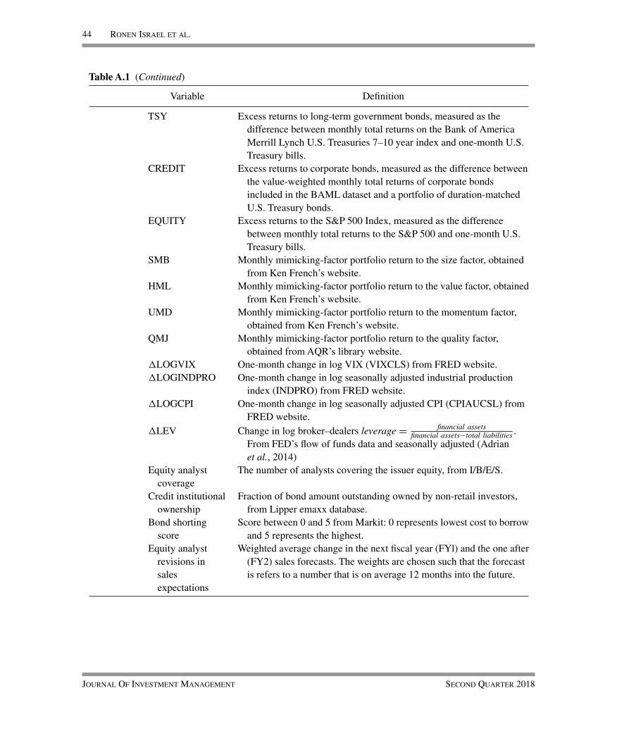
44 Ronen Israel et al.
Table A.1 (Continued)
Variable Definition
TSY Excess returns to long-term government bonds, measured as thedifference between monthly total returns on the Bank of AmericaMerrill Lynch U.S. Treasuries 7–10 year index and one-month U.S.Treasury bills.
CREDIT Excess returns to corporate bonds, measured as the difference betweenthe value-weighted monthly total returns of corporate bondsincluded in the BAML dataset and a portfolio of duration-matchedU.S. Treasury bonds.
EQUITY Excess returns to the S&P 500 Index, measured as the differencebetween monthly total returns to the S&P 500 and one-month U.S.Treasury bills.
SMB Monthly mimicking-factor portfolio return to the size factor, obtainedfrom Ken French’s website.
HML Monthly mimicking-factor portfolio return to the value factor, obtainedfrom Ken French’s website.
UMD Monthly mimicking-factor portfolio return to the momentum factor,obtained from Ken French’s website.
QMJ Monthly mimicking-factor portfolio return to the quality factor,obtained from AQR’s library website.
�LOGVIX One-month change in log VIX (VIXCLS) from FRED website.�LOGINDPRO One-month change in log seasonally adjusted industrial production
index (INDPRO) from FRED website.�LOGCPI One-month change in log seasonally adjusted CPI (CPIAUCSL) from
FRED website.�LEV Change in log broker–dealers leverage = financial assets
financial assets−total liabilities .From FED’s flow of funds data and seasonally adjusted (Adrianet al., 2014)
Equity analystcoverage
The number of analysts covering the issuer equity, from I/B/E/S.
Credit institutionalownership
Fraction of bond amount outstanding owned by non-retail investors,from Lipper emaxx database.
Bond shortingscore
Score between 0 and 5 from Markit: 0 represents lowest cost to borrowand 5 represents the highest.
Equity analystrevisions insalesexpectations
Weighted average change in the next fiscal year (FYl) and the one after(FY2) sales forecasts. The weights are chosen such that the forecastis refers to a number that is on average 12 months into the future.
Journal Of Investment Management Second Quarter 2018

Common Factors in Corporate Bond Returns 45
Acknowledgement
Aprevious version of this paper was titled “Invest-ing with style in corporate bonds.” We thankDemir Bektic, Maria Correia, Wayne E. Fer-son, Patrick Houweling, Antti Ilmanen, SarahJiang, Toby Moskowitz, Narayan Naik, LassePedersen, Kari Sigurdsson and participants at the4th Alliance Bernstein Quant Conference, 24thEuropean Pensions Symposium, 7th Inquire UKBusiness School Meeting, Norwegian Ministryof Finance and University of Cambridge, 2016SFS Finance Cavalcade, London Quant Group,University of Notre Dame and UBS Quantita-tive Investment Conference 2016 for their helpfuldiscussion and comments. We acknowledge theoutstanding research assistance of Peter Diep,Johnny Kang and Mason Liang. The views andopinions expressed herein are those of the authorsand do not necessarily reflect the views of AQRCapital Management LLC (“AQR”), its affiliates,or its employees. This information does not con-stitute an offer or solicitation of an offer, or anyadvice or recommendation, by AQR, to purchaseany securities or other financial instruments andmay not be construed as such.
Notes1 If one of the standardized measures is missing, we assign
a zero score such that the combination will have a non-missing score for the union of names which have at leastone non-missing score.
2 Between January 1997 and December 1998, we set thescalar equal to its value as of January 1999.
References
Adrian, T., Etula, E., and Muir, T. (2014). “Financial Inter-mediaries and the Cross-Section of Asset Returns,” TheJournal of Finance 69(6), 2557–2596.
Altman, E. I. (1968). “Financial Ratios, Discriminant Anal-ysis and the Prediction of Corporate Bankruptcy,” Journalof Finance 23(4), 189–209.
Andersen, T. G., Bollerslev, T., Diebold, F. X., and Ebens,H. (2001). “The Distribution of Realized StockReturn
Volatility,” Journal of Financial Economics 61(1),43–76.
Asness, C. S., Andrea, F., and Lasse, H. P. (2014). “QualityMinus Junk,” Working Paper.
Asness, C., A., Ilmanen, R. I., and Moskowitz, T. (2015).“Investing with Style,” Journal of Investment Manage-ment 13, 27–63.
Asness, C., Moskowitz, T., and Pedersen, L. (2013). “Valueand Momentum Everywhere,” Journal of Finance 68,929–985.
Asquith, P., Au, A. S., Covert, T., and Pathak, P. A. (2013).“The Market for Borrowing Corporate Bonds,” Journal
of Financial Economics 107, 155–182.Asvanunt, A. and Richardson, S. (2017). “The Credit Risk
Premium,” Journal of Fixed Income, Winter 2017.Ben Dor, A., Dynkin, L., Hyman, J., Houweling, P., Van
Leeuwen, E., and Penniga, O. (2007). “DTS (DurationTimes Spread),” The Journal of Portfolio Management33, 77–100.
Bessembinder, H., Maxwell, W., and Venkataraman, K.(2006). “Market Transparency, Liquidity Externalities,and Institutional Trading Costs in Corporate Bonds,”Journal of Financial Economics 82, 251–288.
Bharath, S. T. and Shumway, T. (2008). “ForecastingDefault with the Merton Distance to Default Model,”Review of Financial Studies 21(3), 1339–1369.
Binsbergen, J. H. and Koijen, R. S. J. (2015). “TheTerm Structure of Returns: Facts and Theory,” WorkingPaper.
Bradshaw, M. T., Richardson, S. A., and Sloan, R. G.(2001). “Do Analysts and Auditors Use Informationin Accruals?,” Journal of Accounting Research 39(1),45–74.
Carvalho, R., Dugnolle, P., Xiao, L., and Moulin, P. (2014).“Low-RiskAnomalies in Global Fixed Income: Evidencefrom Major Broad Markets,” The Journal of Fixed Income23, 51–70.
Chen, L., Lesmond, D. A., and Wei, J. (2007). “CorporateYield Spreads and Bond Liquidity,” Journal of Finance62, 119–149.
Chen, N. F., Roll, R., and Ross, S. A. (1986). “EconomicForces and the Stock Market,” Journal of Business 383–403.
Choi, J. and Kim, Y. (2015). “Anomalies and Market
(Dis)integration,” Working Paper, UIUC.Chordia, T., Goyal, A., Nozawa, Y., Subrahmanyam,
A., and Tong, Q. (2016). “Are Capital Market Anoma-lies Common to Equity and Corporate Bond Markets?,”Working Paper, Emory University.
Second Quarter 2018 Journal Of Investment Management

46 Ronen Israel et al.
Cochrane, J. H. (2009). Asset Pricing: (Revised Edition).Princeton University Press.
Correia, M., Richardson, S., and Tuna, I. (2012). “ValueInvesting in Credit Markets,” Review of AccountingStudies 17(3), 572–609.
DeMiguel, V., Garlappi, L., and Uppal, R. (2009). “Optimalversus Naive Diversification: How Inefficient is the 1/NPortfolio Strategy?,” Review of Financial Studies 22(5),1915–1953.
Edwards, A. E., Harris, L. E., and Piwowar, M. S.(2007). “Corporate Bond Market Transaction Costs andTransparency,” Journal of Finance 62, 1421–1451.
Fama, E. F. and Kenneth, R. F. (1993). “Common RiskFactors in the Returns on Stocks and Bonds,” Journal ofFinancial Economics 33(1), 3–56.
Frazzini, A., Israel, R., and Moskowitz, T. J. (2012). “Trad-ing Costs of Asset Pricing Anomalies,” Working Paper,AQR Capital Management.
Frazzini, A. and Pedersen, L. H. (2014). “Betting AgainstBeta,” Journal of Financial Economics 111, 1–25.
Gebhardt, W. R., Hvidkjaer, S., and Swaminathan, B.(2005a). “The Cross-Section of Expected Corporate BondReturns: Betas or Characteristics?,” Journal of FinancialEconomics 75, 85–114.
Gebhardt, W. R., Hvidkjaer, S., and Swaminathan, B.(2005b). “Stock and Bond Market Interaction: DoesMomentum Spill Over?,” Journal of Financial Eco-nomics 75, 651–690.
Grossman, S. J. and Stiglitz, J. E. (1980). “On theImpossibility of Informationally Efficient Markets,” TheAmerican Economic Review 70(3), 393–408.
Haesen, D., Houweling, P., and van Zundert, J. (2013).“Residual Equity Momentum for Corporate Bonds,”Working Paper, Robeco Quantitative Strategies.
Hallerbach, W. G. and Houweling, P. (2013). “Ibbotson’sDefault Premium: Risky Data,” The Journal of Investing22, 95–105.
Harris, L. (2015). “Transaction Costs, Trade Throughs, andRiskless Principal Trading in Corporate Bond Markets,”Working Paper, USC.
He, Z. and Krishnamurthy, A. (2013). “Intermediary AssetPricing,” The American Economic Review 103(2), 732–770.
Hong, H., Lim, T., and Stein, J. C. (2000). “Bad News Trav-els Slowly: Size, Analyst Coverage and the Profitabilityof the Momentum Strategies,” The Journal of Finance55(1), 265–295.
Hotchkiss, E. S. and Jostova, G. (July 9, 2007). “Deter-minants of Corporate Bond Trading: A ComprehensiveAnalysis,” Working Paper.
Houweling, P. and van Zundert, J. (2014). Factor Investingin the Corporate Bond Market,” Working Paper, RobecoQuantitative Strategies.
Jostova, G., Nikolova, S., Philipov, A., and Stahel, C. W.(2013). “Momentum in Corporate Bond Returns,” Reviewof Financial Studies 26(7), 1649–1693.
Kelly, B. T., Manzo, G., and Palhares, D. (2016). “Credit-Implied Volatility,” Manuscript.
Koijen, R., Moskowitz, T., Pedersen, L., and Vrugt, E.(2014). “Carry. Working Paper, University of ChicagoBooth School of Business,” New York University, Uni-versity of Amsterdam.
Kwan, S. H. (1996). “Firm-Specific Information andthe Correlation Between Individual Stocks and Bonds,”Journal of Financial Economics 40, 63–80.
Lewellen, J. (2015). “The Cross-Section of Expected StockReturns,” Critical Finance Review 4, 1–44.
Lok, S. and Richardson, A. (2011). “Credit Markets andFinancial Information,” Review of Accounting Studies 16,487–500.
Merton, R. (1974). “On the Pricing of Corporate Debt: TheRisk Structure of Interest Rates,” Journal of Finance 29,449–470.
Moreira, A. and Muir, T. (2016). “Volatility Managed Port-folios (No. w22208),” National Bureau of EconomicResearch.
Ng, K. Y. and Phelps, B. (2014). “Structure of U.S.Corporate Excess Returns: The Hunt for a ‘Low-Risk’Anomaly,” Working Paper, Barclays.
Novy-Marx, R. (2013). “The Other Side of Value: TheGross Profitability Premium,” Journal of Financial Eco-nomics 108(1), 1–28.
Palhares, D. (2013). “Cash-Flow Maturity and Risk Pre-mia in CDS Markets,” Working Paper, AQR CapitalManagement.
Schaefer, S. M. and Strebulaev, I. A. (2008). “Struc-tural Models of Credit Risk are Useful: Evidence fromHedge Ratios on Corporate Bonds,” Journal of FinancialEconomics 90(1), 1–19.
Shleifer, A. and Vishny, R. W. (1997). “The Limits toArbitrage,” The Journal of Finance 52(1), 35–55.
Shumway, T. (2001). “Forecasting Bankruptcy More Accu-rately: ASimple Hazard Model,” Journal of Business 740,101–124.
Keywords: Corporate bonds; mispricing
JEL Classification: G12; G14; M41
Journal Of Investment Management Second Quarter 2018