Federal Reserve Bank of Dallas Globalization and Monetary Policy Institute

Working Paper No. 154 http://www.dallasfed.org/assets/documents/institute/wpapers/2013/0154.pdf

Commodity House Prices*

Charles Ka Yui Leung

City University of Hong Kong

Song Shi Massey University

Edward Tang

City University of Hong Kong

August 2013

Abstract This paper studies how commodity price movements have affected local house prices in commodity-dependent economies, Australia and New Zealand. We build a geographically hierarchical empirical model and find that commodity prices influence local house prices directly and also indirectly through macroeconomic variables. While commodity price changes function more like “income shocks” rather than “cost shocks” in both Australia and New Zealand, regional heterogeneity is also observed in terms of differential dynamic responses of local house prices to energy versus non-energy commodity price movements. The results are robust to alternative approaches. Directions for future research are also discussed. JEL codes: F40, G10, R30

* Charles Ka Yui Leung, Department of Economics and Finance, City University of Hong Kong, Kowloon Tong, Hong Kong, 852-2788-9604. kycleung@cityu.edu.hk. Song Shi, School of Economics and Finance, Massey University, Private Bag 11 222, Palmerston North, 4442, New Zealand, 64-6-356-9099. Ext. 2692. S.Shi@massey.ac.nz. Edward Tang, Department of Economics and Finance, City University of Hong Kong, Kowloon Tong, Hong Kong, 852-3442-6768. Edward.c.h.tang@gmail.com.. The authors are grateful to many colleagues and friends, especially Nan-Kuang Chen, Xu Han, Dan McMillen, Peng Wang, Isabel Yan, seminar participants of the City University of Hong Kong Brown Bag, Massey University, Southwest University of Finance and Economics, Tsinghua University, Asian Real Estate Society conference, GCREC conference, PRRES conference, for helpful comments and suggestions. The comments and suggestions from anonymous referees lead to significant improvements. The financial support from the City University of Hong Kong and Massey University are gratefully acknowledged. The work described in this paper was partially supported by a grant from the Research Grants Council of the Hong Kong Special Administrative Region, China [Project No. CityU 146112]. Tang acknowledges the financial support from Graduate Student Travel Grant at the City University of Hong Kong. The usual disclaimer applies. The views in this paper are those of the authors and do not necessarily reflect the views of the Federal Reserve Bank of Dallas or the Federal Reserve System.

1 

 

Commodity House Prices

1. Introduction

This paper attempts to contribute to several strands of the literature. First, we intend to

establish that commodity prices, which are arguably determined in the international market, can

influence even the price of non-tradable goods like housing in an open economy. Clearly, the

approach of this research, which is to take the commodity price fluctuations as an “exogenous

shock”, is inspired by Chen and Rogoff (2003). In their study of the relationship between the

commodity prices and exchange rates, Chen and Rogoff (2003, p.133-134) explain that for

some commodity-exporting countries, the shock identification which are in general difficult can

be solved easily. They write,

“The elusive connection between economic fundamentals and exchange rates has been one

of the most controversial issues in international finance,… it has also been recognized that if

one could find a real shock that were sufficiently volatile, one could potentially go a long way

towards resolving these empirical challenges… For most OECD economies, however, it is

difficult to know what the shock might be, much less measure it…. We find that these bilateral

exchange rates do exhibit significant co-movement with world commodity prices… For

Australia, Canada, and New Zealand, because primary commodities constitute a significant

component of their exports, world commodity price movements… potentially explain a major

component of their terms-of-trade fluctuations.”

In this study, we therefore follow Chen and Rogoff (2003) to focus on Australia and New

Zealand. To make the identification problem even easier, this study will focus on the

disaggregate house prices in these countries. The rationale is simple. Houses are clearly non-

traded (and durable) consumption goods and unlikely to serve as an intermediate input for the

production of other goods. The local house prices are also unlikely to have an impact neither on

2 

 

the aggregate economy nor the world market of commodities. All these features suggest that the

causality from the commodity prices to local house prices would be one-directional, which in

turn simplifies the analysis and the interpretation of results.

As observed by Chen and Rogoff (2003), international trade, and especially commodity

trade is a significant part of the export of the two countries.1 In the appendix, we provide more

details and even confirm the Granger causality between international trade and GDP in both

countries. Due to the importance of international trade in general, and commodity trade in

particular, it seems reasonable to conjecture that fluctuations in commodity prices could

significantly affect the total output of Australia and New Zealand. This leads to another point

we attempt to make. In the previous literature on the relationship between commodity prices

and the macro-economy, attention is often focused on oil price.2 In that literature, oil price

fluctuations are often interpreted as “cost shocks” and related to recessions. For commodity-

exporting countries, however, commodity price changes can become “income shocks” and

hence the results could be different. In this paper, we follow Chen and Rogoff (2003) to

separate the energy commodity price index from the non-energy commodity price index. Our

empirical analysis confirms that they have different effects on the macroeconomic variables as

well as on the house prices. It may suggest more caution is needed in modeling “terms of trade

shocks” in the theoretical literature. In particular, there may be a need to carefully separate

energy-related commodity prices from the non-energy-related counterpart.3 As the Australia

and New Zealand currencies can be viewed as the “commodity currency” (Chen and Rogoff,

                                                            1 A specific historical example is the banking crisis between 1890 and 1895. Due to the fall in global commodity prices, it led to a drop in the land prices, putting pressures on the Bank of New Zealand, the main mortgage lender. The government finally rescued the bank in 1895, but it encountered a cost of 1.6% of GDP. See Bordo et al (2010) for more details. For more details of the composition of commodity export in Australia and New Zealand, see the Appendix. 2 Clearly, it is beyond the scope of this paper to survey that literature. Among others, see Hamilton (2008) for a review. 3 There is a very large literature on this issue. For instance, Jones (1979) studies the impact of “terms of trade shock” under different assumptions. Marion (1984) discusses the relationship between oil price increase and non-traded goods. For a discussion of the literature, see Caves et al (1999), Lubik and Teo (2005), Lim and McNelis (2008), among others.

3 

 

2003), this paper shows that local house prices in at least some cities of Australia and New

Zealand can be viewed as “commodity house prices”.

Our data set consists of a panel of house prices from 8 cities in Australia and 17 cities in

New Zealand. It helps to mitigate the potential aggregation bias, which could arise in national

level studies.4 Since the sampling period and the data frequency are different, we will examine

the two countries separately. We also collect national level and regional level data, as much as

we can. They include variables that are typically believed to be influential to the house prices

(such as the GDP, unemployment, interest rate, etc.) as well as variables that are important for

open economies (such as the real exchange rate, capital flow to GDP ratio, debt to GDP ratio,

etc.), subject to data availability at the corresponding house price frequency. Stock price (in real

terms) is also included as it may capture the general market liquidity and sentiment. Table 1a

provides a summary.5

[Table 1a about here]

In addition, this paper tests a simple empirical and hierarchical model of Australia and New

Zealand economy on how shocks could transmit from the national to the regional level. It

highlights a geographically hierarchical propagation mechanism that allows for regional

heterogeneity in response to the same “exogenous shock”. To our knowledge, theoretical work

along this approach is relatively rare. Hence, the empirical results here might provide a

benchmark for future theoretical work.

This paper is also related to an emerging literature which recognizes the influence of

“international market” on “local house prices”. For instance, Bardhan et al (2004) show in a

cross-sectional sample that, other things being equal, a higher city rent is associated with a more

open economy in terms of international trade and capital flow. Bardhan et al (2008) show that

                                                            4 For a discussion of cross-sectional aggregation bias, see Hanushek et al (1996), among others. 5 We follow Chen and Rogoff (2003) to define the real exchange rate as the amount of goods in Australia/New Zealand that can be exchange for 1 unit of U.S. goods. Clearly, one merit of it is the facilitation of comparison.

4 

 

the excess return of a real estate firm in the stock market is negatively correlated to the

economic openness, after controlling national as well as firm factors. This paper complements

these researches by focusing on the local house prices of two commodity-exporting economies,

and explores the nonlinear dynamic effects of commodity prices at the city-level.

The organization of this paper is simple. The next section will present our econometric

framework. Then we will provide more details about our data set, followed by the empirical

results. The last section concludes.

2. Estimation strategies and the empirical models

Since our objective is to investigate whether (and how) the commodity prices, which are

determined in the world market, would impact the local (city-level) house prices in Australia

and New Zealand, our econometric framework needs to be flexible enough to include different

possibilities. The commodity price may affect the macroeconomic variables, which in turn

affects the local house prices. For instance, higher commodity prices may impact the

unemployment rate in general and hence the public finance of the national government. This

may in turn imply a change in the probability of tax increase and it could affect the house price

even at the local level. Higher commodity prices could also means an improvement of the

public finance of the regional government if the region’s economy heavily depends on the

export of the corresponding commodities. It may imply more generous social welfare which

would encourage immigration and be interpreted as positive news to the local housing market.

On the other hand, higher commodity prices could also lead to higher inflation rate in general,

which in turn encourages the central bank to adopt a tighter monetary policy, which tends to

depress the house prices. Since the economic structure and “indebtness” of different regions

tend to be unequal, the local house prices may be affected unevenly. Figure 1 provides graphical

5 

 

illustrations for these possibilities. Since we do not know the empirical relevance of different

channel(s) a priori, we proceed with a three-step procedure which naturally captures these

possibilities with different parameter estimates.

[Figure 1 about here]

Stage one: extracting the effect of commodity prices on national economic variables

For the purpose of the empirical analysis, we conduct our empirical analysis in three

stages. As we want to separate the influence of national and local factors on the housing market

apart from commodity prices, we first study how the aggregate variables of Australia and New

Zealand can be influenced by the international commodity prices. Specially, we run the

following Vector Auto-regressive (VAR) equation for each country separately in the first stage:6

 =   +   +   +   +                 (1) 

where ntV is the vector of national variables at time t that are believed to be important and

would affect the house prices. They include variables that represent the “economic

fundamentals” (i.e. the growth rate of real GDP, the growth rate of national unemployment, the

number of net national migration per 1000 people of existing nationwide population), variables

that would affect investment as well as those represent the financial market (i.e. the change of

real interest rates, the change of log real exchange rates, the change of the real stock price), and

the change of bank loans (in real terms) which is proxy for the credit market condition; ctP is

the vector of commodity prices at time t including energy and non-energy commodity prices;

the residual term will become the “filtered national variable vector”  7. For most variables, we

use the change rather than the level because of the stationarity consideration. In the case of

                                                            6 Recall that the frequency of Australia and New Zealand data are different and hence we need to estimate the models of the two countries separately. 7 It means that it is a vector where the effect from commodity prices on the national variables has been filtered out.

6 

 

Australia, net migration data is not accessible to us. On the other hand, we have access to the

debt-to-GDP ratio as well as the net capital flow-to-GDP ratio. These variables can contribute to

control for the international capital flow, as some authors argue that capital flow can also

influence the house price.

There are two distinctive features of the above equation (1). First, the change of the real

exchange rate is included as a national economic variable. Hence, we are treating the change of

the log real exchange rate as an endogenous variable following Chen and Rogoff (2003). This

formulation will allow the data to inform us whether (and if so, how) the commodity prices

would affect the national economic variables. Second, we add the lagged national variables into

the equation, to capture the persistence of the national variables. Without that, the estimates can

be biased.

Stage two: extracting the effect of commodity prices on local economic variables

At stage two we want to examine if the commodity prices affect the local variables

directly, or only through the national variables. We allow the local variables to depend on the

present as well as past values of filtered national variables and commodity prices. Specifically,

we run the following VAR for city j in each country:

,  =  ,  +   +   +   +   +  ,  +   ,  , j = 1, 2, …8      (2) 

where 0, jB captures the fixed effect of the regional rent, ,rj tV is the vector of regional/local

economic variables for city j. Among the data series accessible to us at the same frequency and

during the same sampling period, there is only one relevant regional/local level variable, i.e. the

                                                            8 In the case of Australia, j=1,2,…,8 and for the case of New Zealand, j=1,2,…,17.

7 

 

rent for city j; the residual term , will become the “filtered regional variable vector” , for

city j.9

Stage three: extracting the effect of commodity prices on house price movements

At this stage we want to examine if the commodity prices affect the local house prices

directly, or only through the national or regional variables. We allow the local house prices to

depend on its past values, the present as well as past values of filtered national variables, the

present as well as past value of filtered city variables, and the present as well as past values of

commodity prices. Specially, we run the following regression for each country:

,  =  ,  +  ,  + ∑ ,  +  +  ,  +   +   + ∑  +  , j = 1, 2, …    (3) 

where ,j tHP is the j-th city house price at period t; , 1k tHP is the k-th city house price (cities

other than j, and hence k j ) at period t-1; 0, jC represents the city fixed effect; S present the

seasonal dummy variables to deal with the seasonal effect in house prices.

It should be noticed that, in spite of its simplicity, the potential effects of commodity prices

can be captured by 1 2,A A at the national level, by 1 2,B B at the regional level, while the total

effect are captured by 4 5,C C at the regional level in this econometric framework.10 Notice that

all these matrices are estimated separately. Hence, this framework would help us to identify and

dictate, if any, the effect of commodity price on the local house prices.

                                                            9 Some seminar participants express the concern that equation (2) may not be able to capture cross-city spill over effect that may exist in the data. In Appendix C, we calculate all pair-wise correlation among city rents, once with spot market commodity price data and again with futures market counterpart. We find that most of the correlations are not statistically significant, and even when they are, their numerical values are around 0.3 or even smaller. 10 See the appendix for a formal proof. We are grateful to an anonymous referee for this point.

8 

 

3. Data Description

This research utilised several data sets. The Australian Bureau of Statistics (ABS) provides

the quarterly median house price data on eight Australian cities as well as the data of other

macroeconomic variables. To match the data of New Zealand, we focus on the period between

1988 and 2011.11 The corresponding city-level quarterly median house rent data is purchased

from Real Estate Institute of Australia (REIA). Previous studies on Australia house price

employ data from the same sources and a comparison of results would be convenient.12

For New Zealand, there is a rich monthly data set of freehold (fee simple) open market

transactions of detached or semi-detached houses for seventeen selected cities between 1994

and 2009. House price movements for the seventeen selected cities were estimated directly from

the transaction data by using Case-Shiller (1987) weighted repeated sale (WRS) method at

monthly intervals, which are unique and not publicly available. The transaction data was

supplied by Quotable Value (QV), the official database for all property transactions in New

Zealand. QV also produces a house price index, but it is on a quarterly basis. Comparing with

the quarterly reported index, our estimated monthly price index will unsmooth the price

movement and increase the number of observations in a time series analysis. Another reason to

estimate house price movement on a monthly basis in this study is because the commodity

prices data are reported on a monthly basis. Forcing the monthly commodity prices into

quarterly counterparts may introduce time aggregation bias. We choose these seventeen cities

because they account well for New Zealand housing stock, as shown in the Appendix A. The

geographic locations of these cities are presented in Figure 2.

< Figures 2a, 2b about here>

                                                            11 The ABS website (http://www.abs.gov.au) provides very detailed explanation on the construction of their house price data and other data series. 12 For instance, see Otto (2007) and the reference therein.

9 

 

Since we have access to transaction-level data in New Zealand, extra efforts have been

invested in the construction of the house price series.13 The local house price indices estimated

as such are then deflated by the consumer price index (CPI) to derive the real house price

indices.

We obtain monthly rental data for detached or semi-detached houses from the Tenancy

Services Division of Department of Building and Housing (DBH) in New Zealand. Under the

Residential Tenancies Act, all tenancy bonds must be lodged with the DBH within 23 working

days from the tenancy start. The bonds normally amount to two or three weeks of rents payable

under the new tenancy. The DBH rental data is transaction based and very comprehensive in

terms of recording the market rent settings for all new residential tenancies in New Zealand. We

first calculate the monthly median rent, and then construct rental indices for each local housing

market. The estimated rental indices are then deflated by CPI and should represent the local

market supply and demand factors for housing.

National economic variables such as real GDP, CPI, population, unemployment rate, and net

migration, are available from Statistics New Zealand.14 For the quarterly reported aggregate

data such as real GDP, CPI and unemployment data, we have interpolated them on a monthly

basis. Monthly net migration is calculated on per 1000 people of the existing population.

Monthly interest rate, exchange rate and bank loan data are obtained from the Reserve Bank of

New Zealand. Stock market price movements are obtained from Datastream. We use the 10-

year government bond rate to represent the interest rate for housing, simply because of the long-

term nature of owning. For the exchange rate, it is expressed as the New Zealand dollar against

                                                            13 For instance, as the repeat sales method is vulnerable to outliers (Meese and Wallace, 1997), we use prior knowledge to eliminate all multiple sales where the second sale price is less than 0.7 or more than 2.5 times the first sale price. Moreover, since the QV data includes building consent information for all the studied cities except Auckland City, we further eliminate the quality changed repeat sales, thus minimizing the constant quality problem faced by the standard repeat sales method. In New Zealand, building consent data is collected for revaluation purposes only where QV is the valuation service provider for the Council. For Auckland City, QV is not the valuation service provider for the council and for that reason there is no building consent data for Auckland City. 14 Notice that for Australia, we are unable to identify accessible dis-aggregate migration data.

10 

 

the US dollar. The interest rate, exchange rate, bank loan and stock prices data are then deflated

by CPI to derive their real terms. In the regression, we follow the literature and use log real

exchange rate.15

Finally, we obtain the commodity prices through various sources. As shown in the appendix,

the composition of commodities being exported from Australia and New Zealand are very

different. To facilitate a comparison of results, we use the relative weights of Chen and Rogoff

(2003) for Australia, whose details are reproduced in the Appendix. For New Zealand, we use

the ANZ export commodity price index, which is expressed in US dollars for spot market non-

energy commodity prices. The ANZ index starts in January 1986 and is reported on a monthly

basis thereafter. The index weights are based on the contributions of each commodity to

merchandise exports in New Zealand and adjusted annually. For spot market energy commodity

prices, we obtain them from Datastream. For robustness check, we have also built our own

futures market energy and non-energy commodity prices  following Chen and Rogoff (2003).

Futures market commodity prices are obtained from Datastream and Global Financial Database.

Due to the data availability our own futures market non-energy commodity price index starts

from January 1998. All commodity prices are then converted into their real terms by the CPI

adjustment.

4. Empirical Results

4.1. Testing for unit roots

It is well known that regressions with non-stationary variables can be spurious.16 Therefore,

we first carry out the unit root tests to all economic variables in order to determine their orders

                                                            15 The rationale is well known. If we define X to be the real exchange rate of the New Zealand goods against the US goods, and run two regressions, ( )Y a bX control U , and ' '(1/ ) ( ) 'Y a b X control U . We will find that in general, 1 / 'b b . On the other hand, if we replace X by ln X , it is easy to show that

'b b and that justifies our log formulation. The same logic applies to Australia.

11 

 

of integration and hence properly de-trend the variables when necessary. Table 1b provides the

full names of the cities and the corresponding short-hand that we are going to use throughout

this paper. Appendix A shows that the 17 cities in our sample represent the majority of both the

population and the number of housing units in New Zealand. It also shows the detailed results

from standard augmented Dickey-Fuller (ADF) test for the time series employed by this study.

It suffices to say that most series are difference-stationary. 17 Thus, we will use the first-

differenced version of those series in our regression.

<Table 1b about here>

4.2. Commodity prices and national economic variables

Our first stage regression estimates the relationship between commodity prices and national

variables (properly de-trended when needed). In general, the national economic variables of

Australia are not as persistent as New Zealand. The details are reserved in the appendix and we

only highlight the effect of commodity prices on national economic variables in Table 2.

<Tables 2a, 2b about here>

Table 2a presents the results of Australia and Table 2b presents the counterpart of New

Zealand. To have a compact presentation, we will put “S” (“F”) in the cell if spot (futures)

market commodity price is found to be statistically significant in influencing the corresponding

variable. Thus, it is possible to have both “S” and “F” in the same cell, or have neither of them

as well. We use + or – to denote whether the relationship is positive or negative.18

Several observations are in order. First, there are some degrees of consistency in the case of

Australia, both energy and non-energy commodity prices would have a positive effect on the

                                                                                                                                                                                              16 Among others, see Hamilton (1994) for a detailed analysis. 17 It means that the original series are non-stationary, but become stationary after first-differencing. See the appendix A for more discussion on this. 18 It is well known that under certain mathematical conditions, point estimates from a linear VAR would coincide with the point estimates that are obtained from each regression running separately. Among others, see Watson (1994) for more details.

12 

 

GDP growth rate and the real interest rate, and a negative effect on the debt-to-GDP ratio. The

real exchange rate is somehow troublesome. When we use spot market commodity prices, we

find that lag energy commodity price is positively correlated to the real exchange rate change

while current period non-energy commodity price is negatively correlated to the real exchange

rate change. In the robustness section, we will examine alternative specifications and study the

overall effect of commodity prices on the local house prices.

Second, using spot market commodity prices may give different results than using futures

market commodity prices. And commodity prices seem to affect different national economic

variables in different countries. For Australia, spot market commodity prices would affect the

change of unemployment, change of real interest rate, change of real exchange rate and change

of real stock price. However, when futures market commodity prices are used instead, the effect

on the change of unemployment rate and change of real stock price will disappear. Instead,

futures market commodity prices are found to influence real GDP growth rate, change of debt-

to-GDP ratio, and net capital flow-to-GDP ratio, in addition to the effect on change of real

interest rate and change of real exchange rate.

For New Zealand, spot market commodity prices are found to influence real GDP growth

rate, change of unemployment rate and change of real interest rate. When futures market

commodity prices are used instead, then only change of unemployment rate and change of real

exchange rate are affected.

There are many potential reasons for the difference in results. First, futures market

commodity prices are not perfect predictors of the subsequent period spot market counterparts.

In addition, the contents of commodity exports vary across countries. Hence, “energy

commodity price index” in different countries has different statistical properties and may

therefore interact with the macroeconomic variables differently. Perhaps more importantly, the

13 

 

participation in spot versus futures market is different. Limited by space, we reserve the details

in the appendix.

In sum, the results from Tables 2a and 2b have supported our hypothesis that commodity

prices have an effect on national economic variables. We now proceed to the next stage of the

regression, which examines whether commodity prices would impact the regional economic

variables, controlling for the national variables.

4.3. Commodity prices and local economic variables

Our second stage regression estimates the impact of commodity prices on local economic

variables such as the local housing market rent, controlling for the effect of the national

economic variables. To achieve this, we used the “commodity price-filtered” national variable

from the first stage regression in our second stage regression. Again, the details are reserved in

the appendix and we only highlight the impact of commodity prices on local rent in Table 3.

And to facilitate the comparison, our notations in Table 3 are consistent with that in Table 2.

<Tables 3a, 3b about here>

Table 3a presents the results in Australia. It is clear that when spot market commodity prices

are used, none of the city rent series is affected by the commodity prices. When futures market

commodity prices are used instead, the effect on rent in Adelaide, Brisbane, Darwin and Perth

are all in-significant. Decisive results come from Canberra and Sydney, where lagged non-

energy commodity price is found to exert a positive and statistically significant effect on the

rent. While lagged energy commodity prices impact the rent in Hobart negatively, the lagged

non-energy commodity prices impact the rent in Hobart positively. The case of Melbourne is a

bit confusing. While current period non-energy commodity price has a negative effect on the

rent in Melbourne, the lagged non-energy commodity price carries a positive effect. This could

be due to the fact that there may be relatively more financial market participation in Melbourne

14 

 

and the landlords and renters may not hedge on the same side. Unfortunately, we do not have

access to personal financial portfolio to verify this conjecture and can only leave these for the

future research to pursue.

The case of New Zealand is very clear. For most cities, their rents are affected by neither

spot market nor futures market commodity prices. For the spot market, only the non-energy

commodity price can affect (positively) the rent in North Shore and Manukau. For futures

market, the energy commodity price affects (negatively) the rent in Hamilton and Palmerston

North.

In sum, our second stage regression does not perform as good as the first stage. One

possibility is that there are strong correlations among the rents in different cities and our

formulation does not capture that. In the appendix, however, we show that the rents among

different cities in Australia, as well as among those in New Zealand are not significantly

correlated in general. And for those pairwise correlations that are statistically correlated, the

numerical values typically do not exceed 0.3, which suggests that the correlations are really not

that strong.19 An alternative explanation is that the rental market adjusts slowly and hence it

would react to further past (rather than immediately past) of the aggregate economy. However,

our sample is relatively short and does not allow for including more lags in the regression with

all these filtered variables. It is also possible that the rent is determined by some other variables

such as the bargaining power between the landlords and tenants. Unfortunately, among the

dataset accessible to us, we do not have the appropriate variable to capture that.

                                                            19 And since they are not very strongly correlated, even if we replace the filtered macroeconomic variables by some “common factors” or principal components, it may not improve the results significantly.

15 

 

4.4. Commodity prices and local house prices

Our third stage regression attempts to quantify the effect of commodity prices on local

house prices. For the interest of the space, we would first present the results from pooled

regression. And we will then highlight some findings when the city-level house prices are

regressed individually. Tables 4a and 4b present the results when local house prices are pooled

and regressed against commodity prices, the filtered national variable from the first stage

regression, and filtered and pooled local economic variables (rents) from the second stage

regression. Since seasonality is an important feature for the house prices in both countries, we

have added the quarterly seasonal dummies for the regression of Australia and monthly seasonal

dummy variables for the case of New Zealand.

<Tables 4a, 4b about here>

In Table 4a, the dependent variable is the city-level house price in Australia. The first

column presents the results when spot market commodity prices are employed and the second

column presents the results when futures market commodity prices are used instead. The results

in the two columns are consistent with each other. The signs of the coefficients are typically the

same, and even the numerical values are close in many cases. First, it is clear that the lag real

house price change has a positive effect on the current period house price change, which is often

termed as “momentum effect” in the literature. The magnitude is about 0.3 and hence it is not

that large. The signs of the estimated coefficients are mostly expected. Unemployment has a

negative effect on house price because a higher unemployment would mean fewer buyers and

more sellers in the market, which would depress the house price. External debt and net capital

flows have positive effects on the house price as buyers are borrowing from abroad, probably

through financial intermediations and compete for houses, and the house price rises as a result.

City level rent has a positive effect on the house price because rent is an indicator of the cash

16 

 

flow that house-investors would receive and it seems reasonable to expect that the two are

positively correlated. A seasonal dummy is statistically significant as well.

In the appendix, we illustrate that the coefficients for the commodity prices would be the

total effect of the commodity prices on the local house prices, when (filtered) national variables

as well as (filtered) city level rent are used as control. Table 4a suggests that energy commodity

price has no impact on the local house price. On the other hand, non-energy commodity price in

the spot market has a positive effect on house price. In the appendix, we conduct the regression

on each city’s house price on the same set of explanatory variables separately, and find that the

result is mainly driven by three cities: Adelaide, Canberra and Perth. This result may not be

surprising given the economic structure of these cities. For instance, in the state of Western

Australia, where Perth is located, the gross state value added is about 236 billion Australian

dollars in the year 2011-12, where Mining alone contributes 83 billion (Australian Bureau of

Statistics, 2012). It seems reasonable to expect that commodity price fluctuations can have

significant impact on the local house prices.

Table 4b shows the results of New Zealand, which are similar. The results of using spot

market and futures market commodity prices are similar qualitatively, and the results are

quantitatively more significant with spot market prices. National variables such as migration,

real interest rate, real exchange rate, real bank loans, as well as local variables such as local

house rents all have statistically significant impacts on local house prices. The effect of non-

energy commodity price on local house price is also positive and statistically significant. In the

appendix, we report the results that each city’s house price is estimated separately. We find that

the non-energy commodity prices are influential to the house prices in four cities, Auckland,

Hamilton, Manukau and Wellington. The appendix also shows that Auckland and Manukau

alone constitute almost 20% of the whole country’s population. Thus, it seems reasonable to

17 

 

conclude that the commodity price movements are indeed important for house price movement

in New Zealand, at least to a significant part of the population.

Comparing Tables 4a and 4b, we find two obvious differences. First, the sign of previous

house price change is positive in Table 4a, but becomes negative in Table 4b. The results

suggest that house price movements in New Zealand display some kind of mean reversion. It

can be due to the fact that our estimation results of Australian are based on quarterly data while

that of New Zealand are from monthly data. The variations in the institutional settings (such as

the real estate agency regulations, the bank loan application and approval procedures, etc.), the

conduct of monetary policy (for instance, how strict the central bank follows the “inflation-

targeting policy”) as well as economic structure may also contribute to the difference in

estimation results.

Interestingly, real interest rates are positively correlated to real house price changes both in

Australia and New Zealand. This may be related to the inflation-targeting monetary policy

adopted by the two countries. For instance, let us consider a positive productivity shock. It will

lead to a higher economic growth rate in the short run and possibly a higher inflation rate. In

response to that, the central bank would increase the nominal interest rate aggressively so that

the real interest rate also increases.20 At the same time, a positive productivity shock would also

stimulate the housing demand. Since the housing supply is almost inelastic in the short run, the

house price would also increase. This could lead to a positive correlation between the interest

rate and the house price. However, there may be more than one reason why the real interest rate

and the house price are positively correlated, and we leave this to future research for further

investigation.

                                                            20 This is related to the Taylor Principle in the literature on monetary policy. The literature is too large to be reviewed here. See the textbook by Walsh (2010), among others.

18 

 

Perhaps more importantly, we find that, once we control for the effect of the

macroeconomic and local economic variables, energy commodity prices are not important in

determining the local house prices, both in Australia and New Zealand. This result holds

whether we use spot market or futures market commodity prices. On the other hand, non-energy

commodity prices have statistically significant and positive effect on the local housing prices.

Again, the result holds whether we use spot market or futures market commodity prices. These

results seem to be intuitive. For Australia, the export of energy commodities used to be less than

20% of total export until recent years. For New Zealand, most exports are non-energy

commodities. Hence, an increase in the non-energy commodity prices would have a similar

effect as a positive productivity shock, which would encourage the local house prices to

increase. It confirms our earlier conjecture that commodity price shock can function like a

positive “income shock” to the local house prices, rather than a negative “cost shock” as

emphasized by some previous literatures. Since the effect of energy commodity prices and the

non-energy counterpart generate very different results, this paper also confirms the findings of

Chen and Rogoff (2003) that it is important to consider the two commodity prices separately. In

particular, our empirical results seem to suggest that energy commodity prices seem to have a

larger effect on the macroeconomic variables, and yet at the end have an almost neglectable

overall effect on the local house prices, while non-energy commodity prices seem to affect the

local house price directly. Thus, our results seem to justify our conjecture that the local house

prices of some of the cities in Australia and New Zealand are “commodity house prices” as their

currencies are “commodity currencies”.

4.5. Dynamic Analysis

In this section, we would investigate how a change in the commodity prices would affect the

local house prices. An obvious candidate is the traditional impulse response analysis (IRA).

19 

 

However, since commodity prices are exogenous variables in our econometric model, strictly

speaking, we cannot apply the traditional IRA. Nonetheless, the simple structure we adopted

here allows us to study the dynamic effect of (global) commodity price change on the city-level

house prices.21 The following proposition formalizes the idea.

Proposition 1

Based on the regression equation (1), (2) and (3), we can derive the following formula,

                   (4)

where L is the lag operator, and hence we can describe how an once-and-for-all change in the

commodity prices, ctP , would affect the local house prices.

(The proof and the details formulas for the matric polynomials, iC L , 1,2,...i can all be

found in the Appendix ).

Equipped with these formulas, we can analyse how a change in the commodity prices would

affect the local house prices. For instance, to investigate how a change in the energy commodity

price would affect the local house price, we simply set ∆ , where is the

standard deviation of the de-trended energy commodity price . Clearly, this is in parallel

to the traditional IRA, where the innovation term would be taken as a standard deviation of the

shock. Similarly, we obtain the effect of non-energy commodity prices on house price changes

by setting ∆ . As an illustration, we will only present the case of one standard

deviation increase in the spot market commodity prices, and the case for futures market

counterpart can be studied similarly. We also follow the IRA tradition to “normalize”, which is

to divide the estimated house price change by the mean of the same city house price to facilitate

comparison across cities. We will present the dynamic responses of the city level house prices

                                                            21 A merit of this approach is that since commodity prices are exogenous variables in the system, we may not worry so much about whether the innovation in the commodity prices are structural shocks or not.

20 

 

of all 8 cities of Australia. For the case of New Zealand, since it is too burdensome to study the

impacts of 17 cities, we will focus the three major cities of New Zealand, Auckland (AK),

Wellington (WT) and Christchurch (CH).22 The results are presented in Figure 3.

<Figures 3a, 3b about here>

In Figures 3a and 3b, y-axis plots the percentage change of house price, ∆ , / in

Australia and New Zealand respectively, where is simply the time-average of , . The

idea is to measure whether the change in house price due to a commodity price change is

economically significant. The x-axis is the time periods (months). To facilitate the comparison,

we plot the responses of city-level house prices to change in energy commodity price as well as

non-energy commodity price in one graph. Several observations are immediate from Figure 3a.

First, in terms of percentage change, in most of the Australian cities, the responses to non-

energy commodity price are much bigger than the energy counterpart, consistent with our

results in Table 4a. Second, in most of the Australian cities, an increase in the energy

commodity price typically generates a hump-shape response in house price, i.e. the house price

will first increase and then decrease. This is somehow similar to what the business cycle

literature found with “productivity shock”. Perth is an exception. Its house price will drop first

and then bound back. It may be related to the fact that Perth may be economically and

geographically different from other cities.

Notice that the local house prices typically “overshoot” in response to an increase in the

non-energy commodity price, i.e. the initial positive effect on house price generated by the

“shock” will die off over time, even becomes a negative response in house price, and then

                                                            22 Previous studies have shown that the house prices in these three cities have a significant effect in affecting the counterparts in smaller cities of New Zealand. Among others, see Shi, Young and Hargreaves (2009). In the appendix, we also apply our dynamic analysis on all 8 cities of Australia and find that the same results hold quantitatively as well.

21 

 

restore to “normal”.23 Such “over-shooting” behaviour is different from that in the exchange

rate market. In the international finance literature, it is well-known that when the nominal prices

are sticky in the short run, the exchange rate may over-shoot, meaning that the short run

adjustment is more than the long run adjustment. Here the key is instead the sluggish housing

supply. Since the supply of housing cannot adjust quickly to a positive commodity price shock

(as an income shock), the local house price increases. Over time, new housing supply arrives at

the market and drives down the house price.24

Figure 3b shows the case of the 3 selected cities in New Zealand. It is clear that they behave

very differently. For instance, an increase in non-energy prices will generate a hump-shape

response in the local house price all three cities, Auckland, Wellington, and Christchurch. On

the other hand, when there is a positive shock in the energy commodity price, the local house

prices of the three cities behave very differently. In Auckland, a momentum of positive

responses will build up and then die off, which is qualitatively like a mirror image of the

response to non-energy commodity price shock. For Wellington, the response to energy

commodity price is qualitatively similar to the response to non-energy commodity price shock,

except that the magnitude will be much smaller. For Christchurch, the house price responses to

both energy and non-energy commodity prices are very similar, both qualitatively and

quantitatively. These differences in house price responses may be due to the differences of the

city economies. Auckland is the largest city of New Zealand and a large share of local economy

is related to commercial activities, including the trading of energy-related commodities.

Wellington is closely linked to government agency and surrounding industrial production. On

the other hand, Christchurch is largely agricultural orientated.

                                                            23 We are aware that Hobart is an exception. We lack more detailed city level data to investigate the reason, and can only leave this to future research. 24 Among others, see Malpezzi and Wachter (2005), Leung (2007) for more discussion on this.

22 

 

In sum, we can conclude that the house price dynamics driven by a change in energy

commodity price can be very different from that generated by the non-energy counterpart,

depending on the local economic structure. And we find that similar patterns emerge from both

Australian and New Zealand cities, which are somehow commodity-export dependent. This

may be worth further attention for theoretical modelling. Obviously, this research benefits a lot

from using 8 Australian and 17 New Zealand cities in the analysis. In other words, our

hierarchical and dis-aggregate approach may help us to uncover the mechanism through which

the global commodity market affecting local house prices.

These observations are clearly at odds with traditional RBC (Real Business Cycles) type

models where there is only one shock which drives the economy. At the same time, they seem

to give support to the approach of DSGE model, which emphasizes the differential responses of

the economy under different shocks.25 In addition, this paper adds weight to the position that we

should analyse the effect of energy-related commodity price shocks separately from the non-

energy-related commodity price shocks.

5. Robustness checks

5.1 What does “filtering” do to the data?

This section attempts to accomplish a few tasks. First, we will show that our approach of a

3-stage regression is indeed important. As a starting point, we first compare the raw data series

with the “filtered” counterparts. When we “filter” or “remove” the effect of commodity prices

on the national or regional economic variables, do we change the behaviour of those variables

significantly? To put it in another way, if the raw data and the filtered data are very similar, then

whether regressing the raw data or filtered data in the second and third stage would not make

                                                            25 Again, the literature is too large to be reviewed here. Among others, see Lim and McNelis (2008) for more discussion.

23 

 

much difference and hence the 3-stage regression approach proposed here may have limited

value-added. Table 5 shows the correlation between the raw data and the filtered data. Notice

that while we have only one raw data series, our models generated two filtered data series, one

is the residual term when the national economic variables are regressed against spot market

commodity prices, and another is when the national economic variables are regressed against

futures market commodity prices (see Table 2). Therefore we can calculate the correlations

between the raw data and the data series filtered by spot market commodity prices, as well as

that between the raw data and the data series filtered by futures market commodity prices. The

two correlations are reported in two different columns in Table 5.

<Tables 5a, 5b about here>

First, whether we filter the data with spot market data or futures market data does not make

very significant difference for both Australia and New Zealand. Second, it seems that different

national variables show very different results. For instance, in the case of Australia, Table 5a

shows that the correlations between the raw and filtered data of GDP growth rate,

unemployment, and debt-to-GDP ratio are below 0.7, suggesting that they may be exposed more

to changes in the commodity prices. For real interest rate change and real exchange rate change,

the correlations are between 0.7 to 0.8, suggesting that they may be less influenced by the

commodity price movements. For the stock price, bank loans and capital flow-to-GDP ratio, the

correlations are 0.9 or above, suggesting that they are almost immune to the fluctuations of the

commodity prices. The correlations among the raw data and the commodity price-filtered-data

of most regional rental change are between 0.7 to 0.9 (except Sydney), suggesting the

commodity prices on these variables are mild. The difference in these correlations also provide

further hints on the channels through which the commodity prices fluctuations in the

international market are translated into local house price movements.

24 

 

A comparison of Tables 5a and 5b might suggest that these channels may be country-

specific. Table 5b shows that the correlations among the raw and filtered data for different

national level variables of New Zealand. It is clear that while the correlations are still below 0.7

for unemployment, the correlations are above 0.8 for GDP growth, which is very different from

the case of Australia. At the same time, the correlations for net migration are below 0.7 and that

for bank loans are around 0.7, suggesting that commodity price fluctuations may affect the local

house price through changing these variables. On the other hand, real interest rate change, real

exchange rate change and real stock price change do not seem to be affected by the filtering of

commodity prices, as the corresponding correlations among the raw and filtered data are close

to or above 0.9. And for most regional rental changes, the correlations among the raw data and

the commodity price-filtered-data are in the range of 0.8 to 0.9. It suggests a minor impact of

the commodity prices to these regional variables.

To shed further light on the exact effects of the filtering procedure on the data series are, we

calculate the serial correlations of all three series: the raw data, the data series filtered by spot

market commodity prices, and the one filtered by futures market commodity prices, and report

the results in Tables 6a and 6b.

Several “stylized facts” are obvious. The raw data are significantly correlated and that

justifies the inclusion of lagged terms in the regressions.26 On the other hand, the filtered data of

Australia are not serially correlated in general, whether the data is filtered by spot commodity

prices or futures commodity prices. For New Zealand, some of the national level data are still

serially correlated after filtering. Yet although the correlations may be statistically significant,

                                                            26 For Australia, the real GDP growth, unemployment rate change, real net debt change are all positively correlated intertemporally, while the real exchange rate change is positively correlated with its own lag. For New Zealand, the list is even longer. Real GDP growth, unemployment rate change, net migration, real interest rate change, real exchange rate and real bank loan change are all positively correlated with their own lags. It should be noticed that the Australian data in our sample are in quarterly frequency and that in New Zealand are in monthly frequency and hence a direct comparison may need extra cautions.

25 

 

their numerical values are around 0.2 or less. Thus, the filtering process significantly reduces, or

even removes, the autocorrelation in the national level variables in Australia and New Zealand.

<Tables 6a, 6b about here>

5.2 Raw data versus filtered data

The previous section studies the effect of filtering onto the national and regional economic

variables. It seems natural for this section to re-examine the effect of commodity prices on the

local house prices if the raw data, instead of the filtered version, have been used in the analysis.

Thus, our robustness check continue to use the (city-level) local house prices as dependent

variable and we compare the results of using the raw data, adding the lagged filtered variable in

equation (3) and (later) by treating the exchange rate as an exogenous variable with the 3-stage

regression approach proposed by this paper. To facilitate the comparison, we reproduce the

results in Table 4 as the first two columns of Table 7. In the third and the fourth columns of

Table 7, we use the raw data instead of the filtered ones. The results of Australia are reported in

Table 7a and those of New Zealand in Table 7b. With this side-by-side comparison, several

observations are in order. First, in general, the effects of macroeconomic variables on the local

house prices are similar. Second, the statistical significance of the local house rent is much

weakened (for the case of Australia) or even disappear (for the case of New Zealand) when the

raw data rather than the filtered data is used. Thus, using our 3-stage regression approach does

alter the economic conclusion. Third, the energy commodity prices do not seem to matter for

local house prices, whether in Australia or in New Zealand. Fourth, the effect of non-energy

commodity prices seems to be the same for Australia. For New Zealand, as evident in Table 7b,

the point estimate for the effect of non-energy commodity prices are significantly reduced. For

the case of spot market non-energy commodity prices, the estimated coefficient drops from

26 

 

0.0855 (3-stage regression) to 0.0582 (raw data). For the futures market counterpart, the

estimated coefficient drops from 0.0465 (3-stage regression) to 0.0295 (raw data). These

observations again confirm the general finding that it is indeed important to use a multi-step

procedure to estimate the effect of international commodity price on the local house price.

<Table 7a, 7b about here>

The fifth and sixth columns of Table 7 present the results after including the lagged variable

of filtered data in equation (3) (see the columns under Eq. (3) – lag). Again, Table 7a presents

the results for Australia and Table 7b for New Zealand. Interestingly, the city rent becomes

statistically significant again, and most estimated coefficients are similar. Overall, all these

suggest that our filtering procedure is indeed important to uncover the relationship between

commodity prices and city-level local housing prices in New Zealand.

5.3. Exogenous versus endogenous exchange rate

We also modify the original formulation and re-run all the regressions as a robustness

check. Specifically, the modified formulation treats the exchange rate as an exogenous variable

instead of an endogenous variable, which is the case considered earlier. This change in

formulation is motivated by the results in Chen, Rogoff and Rossi (2010) that “commodity

currency exchange rates have surprisingly robust power in predicting global commodity prices,”

yet the “reverse” relationship (commodity prices forecasting exchange rates) is less robust.

Formally, our modified model is written as follows:

 =   +   +   +   +   +                                                              (7) 

where the change of log real exchange rate, tE , is no longer included in the vector of national

variables ntV , but instead is included on the right hand side as an exogenous variable.

Similarly, we will have the second stage regression as follows:

27 

 

,  =   +   +   +   +   +   +  ,  +   ,  , j = 1, 2, …       (8) 

And then in the third stage, we have

,  =  ,  +  ,  + ∑ ,  +  +  ,  +   +   + ∑  +  ,  

j = 1, 2, …                                                                                                                                       (9)

Now we have to control for the persistence of house price, , for the filtered national

variables, , for the commodity prices, for the change of the log real exchange rate,

which should cover all different possibilities.

The last two columns of Tables 7a and 7b present the results when the changes of log real

exchange rates are treated as an exogenous variable (see the column under Eq. (3) – exch.

exogenous). Again, except for the point estimate of the effect of non-energy commodity price in

the futures market on the local house price, the results are similar to the original estimation (the

first and second columns). For the case of Australia, the coefficient of the spot market non-

energy commodity price changes from 0.0183 (when exchange rate is treated as an endogenous

variable) to 0.0215 (when the exchange rate is treated as an exogenous variable). For the case of

New Zealand, the change is more significant. The coefficient of the spot market non-energy

commodity price changes from 0.0855 (when exchange rate is treated as an endogenous

variable) to 0.0629 (when the exchange rate is treated as an exogenous variable), while

maintaining 1% significant level.

Putting all these together, we can safely conclude that the influence of the commodity prices

on at least some cities in Australia and New Zealand local house prices are significant and

robust. In addition, our 3-stage estimation procedure contributes in uncovering such a

relationship.

6. Concluding Remarks

28 

 

Commodity price movements have gained attention in international media such as Wall

Street Journal, Financial Times, Economist magazine, etc. They are often perceived as problems

to be solved. Recent researches such as Chen and Rogoff (2003), Chen, Rogoff and Rossi

(2010), amongst others, take advantage of those movements and use them to enhance our

understanding of the business cycles in some “commodity dependent economies”. This paper

follows this approach and uses the commodity price movements to identify the mechanism for

“external shocks” to affect the local house prices. We develop a simple, geographically

hierarchical empirical model for Australia and New Zealand economies as well as their cities.

We find that an increase in commodity prices tend to function like a positive “income shock” to

these commodity dependent economies which would increase the economic growth rate and

suppress the unemployment rate, rather than a “cost shock” which tends to have the opposite

effect. We also derive analytical results to capture the dynamic responses for commodity prices

to influence the local house prices. We find that commodity prices are important to local house

prices. In particular, energy commodity price shocks tend to affect the movement of

macroeconomic variables, while non-energy commodity price shocks tend to affect the local

house prices more directly. Significant regional heterogeneity is also recognized. It is also

important to separate the price shocks from energy commodities from non-energy commodities.

Notice that our model can also be interpreted as the reduced form of a model in which

economic policy; whether in the form of monetary or fiscal (both at the national and regional

level) depends on the commodity prices and economic variables. We formalize such an idea in

the appendix. An implication is that our estimated coefficients become a mixture of the

coefficients in the “policy reaction functions” and the “genuine economic fundamentals”. Thus,

29 

 

future works may further explore how we could separate the possible (endogenous) policy

effect from the pure economic response of the market.27

Clearly, future research can be extended in other directions as well. First, we can follow

Chen and Rogoff (2012) to cover more countries and examine how commodity prices may

affect the exchange rates in different countries. We also notice that the local house price

responses to commodity price shock seem to depend on the local economic structure. Thus,

future research may investigate a more formal way to categorize and quantify such differences

and may thus build a deeper linkage between real estate researches to regional economic studies.

In addition, our empirical results can be taken as “stylized facts” which would inform

further theoretical modelling, for instance, along the line of open economy DSGE models. The

geographically hierarchical empirical model developed here can be modified for other

“exogenous shocks” and applied to other economies. In fact, our modelling strategy may also

suggest a deeper linkage between house price movements which is traditionally studied in the

field of “urban economics” and international asset pricing, which is traditionally studied in the

field of “international finance”. The globalization may have changed the trade barriers among

countries, as well as the research barriers among fields.

                                                            27 Among others, see Bernanke and Blinder (1992), Bernanke and Mihov (1998) for more discussion on this point.

30 

 

References

Aizenman, J. and Y. Jinjarak, 2009. Current account patterns and national real estate markets. Journal of Urban Economics, 66(2), 75-89.

Alexander, C. and M. Barrow, 1994. Seasonality and cointegration of regional house prices in

the UK. Urban Studies, 31(10), 1667–1689.

Alquist, R. and L. Kilian, 2010. What do we learn from the price of crude oil futures? Journal of Applied Econometrics, 25(4), 539-573.

Australian Bureau of Statistics, 2012. 2011-12 Australian national accounts—state accounts. Downloaded from www.abs.gov.au

Bardhan, A. D., R. H. Edelstein and C. Leung, 2004. A note on globalization and urban

residential rents. Journal of Urban Economics, 56(3), 505-513. Bardhan, A. D., R. H. Edelstein and T. Tsang, 2008. Global financial integration and real estate

security returns. Real Estate Economics, 36(2), 285-311. Bernanke, B. and A. Blinder, 1992. The Federal Funds rate and the channels of monetary

transmission. American Economic Review, 82(4), 901-921. Bernanke, B. and I. Mihov, 1998. Measuring monetary policy. Quarterly Journal of Economics,

113(3), 869-902. Bodenstein, M., L. Guerrieri and L. Kilian, 2012. Monetary policy responses to oil price

fluctuations. University of Michigan, mimeo.

Bordo, M. D., D. Hargreaves and M. Kida, 2010. Global shocks, economic growth, and financial crises: 120 years of New Zealand experience. NBER Working Paper No. 16027.

Calvo, G. A., 1983. Staggered prices in a utility-maximizing framework. Journal of Monetary

Economics, 12(3), 383-398. Case, K. E. and R. J. Shiller, 1987. Prices of single-family homes since 1970: new indexes for

four cities. NBER Working Paper No. 2393. Catao, L. and R. Chang, 2012. Monetary rules for commodity traders. Rutgers University,

mimeo.

Caves, R., J. Frankel and R. Jones, 1999. World trade and payments: an introduction. New York: Addison-Wesley.

Chen, Y. and K. Rogoff, 2003. Commodity currencies. Journal of International Economics, 60(1), 133–169.

Chen, Y. and K. Rogoff, 2012. Are the commodity currencies an exception to the rule? Global

Journal of Economics, 1, 1250004 (28 pages).

31 

 

Chen, Y., K. Rogoff and B. Rossi, 2010. Can exchange rates forecast commodity prices? Quarterly Journal of Economics, 125(3), 1145–1194.

Coleman, A. and J. Landon-Lane, 2007. Housing markets and migration in New Zealand, 1962-

2006. Discussion Paper No. DP2007/12. Wellington, New Zealand: Reserve Bank of New Zealand.

Cooley, T. and M. Dwyer, 1998. Business cycle analysis without much theory: a look at

structural VARs. Journal of Econometrics, 83(1-2), 57-88. Davidoff, T., 2006. Labor income, housing prices, and homeownership, Journal of Urban

Economics, 59(2), 209-235. De Gregorio, J., 2012. Commodity prices, monetary policy and inflation. Universidad de Chile,

mimeo. Franses, P.H., 1990. Testing for seasonal unit roots in monthly data. Rotterdam: Econometric

Institute Report No. 9032/A, Erasmus University. Franses, P. H., 1991. Seasonality, nonstationarity and the forecasting of monthly time series.

International Journal of Forecasting, 7, 199–208. Hamilton, J., 1994. Time series analysis. Princeton: Princeton University Press. Hamilton, J., 2008. Oil and the macroeconomy, in New Palgrave Dictionary of Economics, 2nd

edition, ed., by Durlauf, S., Blume, L., New York: Palgrave McMillan. Hanushek, E., S. Rivkin and L. Taylor, 1996. Aggregation and the estimated effects of school

resources. Review of Economics and Statistics, 78(4), 611-627.

Jones, R., 1979. International trade: essays in theory. New York: North Holland.

Kan, K., 2002. Residential mobility with job location uncertainty. Journal of Urban Economics, 52(3), 501–523.

Kan, K., 2003. Residential mobility and job changes under uncertainty. Journal of Urban

Economics, 54(3), 566–586. Leung, C. K. Y., 2004. Macroeconomics and housing: a review of the literature. Journal of

Housing Economics, 13(4), 249-267. Leung, C. K. Y., 2007. Equilibrium correlations of asset price and return. Journal of Real Estate

Finance and Economics, 34(2), 233-256. Lim, G. C., and P. D. McNeils, 2008. Computational macroeconomics for the open economy.

Cambridge: MIT Press. Lubik, T. and W. Teo, 2005. Do world shocks drive domestic business cycles? Some evidence

from structural estimation. Economics Working Paper Archive No. 522. Johns Hopkins University, Department of Economics.

32 

 

Malpezzi, S. and S. Wachter, 2005. The role of speculation in real estate cycles, Journal of Real Estate Literature, 13, 143-164.

Marion, N., 1984. Nontraded goods, oil price increases and the current account. Journal of

International Economics, 16(1-2), 29–44. Meese, R. and N. Wallace, 1997. The construction of residential housing price indices: a

comparison of repeated sales, hedonic regression, and hybrid approaches. Journal of Real Estate Finance and Economics, 14(1-2), 51–74.

Otto, G., 2007. The growth of house prices in Australian capital cities: what do economic

fundamentals explain? Australian Economic Review, 40(3), 225-238. Pindyck, R., 2001, The dynamics of commodity spot and futures markets: a primer. Energy

Journal, 22(3), 1-29.

Reichsfeld, D. and S. Roache, 2011. Do commodity futures help forecast spot prices? IMF working paper.

Rogoff, K., 2001. Dornbusch’s overshooting model after 25 years. Mundell-Fleming Lecture, IMF.

Sargent, T., 1979. Macroeconomic theory. New York: Academic Press. Shi, S., M. Young and B. Hargreaves, 2009. The Ripple effect of local house price movements

in New Zealand. Journal of Property Research, 26(1), 1–24.  

Sockin, M. and W. Xiong, 2013. Feedback effects of commodity futures prices. Princeton University, mimeo.

Walsh, C., 2010. Monetary Theory and Policy, 3rd. ed., Cambridge: MIT Press.

Watson, M., 1994. Vector autoregressions and cointegration, in Handbook of Econometrics, Vol. 4, ed. By R. F. Engle and D. L. McFadden, New York: Elsevier, 2843-2915.

33 

 

Figure 1: The mechanism for the commodity price shock to affect the local house prices

34 

 

Figure 2a: Geographic locations of 8 selected cities of Australia

Figure 2b: Geographic locations of 17 selected cities of New Zealand

35 

 

Figure 3a: Dynamic Response analysis for one standard deviation of spot market commodity prices on 

city level housing prices – Australia

-1

0

1

2

3

4

5

6

1 2 3 4 5 6 7 8 9 10 11 12 13

Energy commodity pricesNon-energy commodity prices

Adelaide

-1.2

-0.8

-0.4

0.0

0.4

0.8

1 2 3 4 5 6 7 8 9 10 11 12 13

Energy commodity pricesNon-energy commodity prices

Brisbane

-1.2

-0.8

-0.4

0.0

0.4

0.8

1.2

1 2 3 4 5 6 7 8 9 10 11 12 13

Energy commodity pricesNon-energy commodity prices

Canberra

-.10

-.05

.00

.05

.10

.15

.20

.25

1 2 3 4 5 6 7 8 9 10 11 12 13

Energy commodity pricesNon-energy commodity prices

Darwin

-.3

-.2

-.1

.0

.1

.2

.3

.4

1 2 3 4 5 6 7 8 9 10 11 12 13

Energy commodity pricesNon-energy commodity prices

Hobart

-2.5

-2.0

-1.5

-1.0

-0.5

0.0

0.5

1.0

1 2 3 4 5 6 7 8 9 10 11 12 13

Energy commodity pricesNon-energy commodity prices

Melbourne

36 

 

-0.4

-0.2

0.0

0.2

0.4

0.6

0.8

1.0

1.2

1 2 3 4 5 6 7 8 9 10 11 12 13

Energy commodity pricesNon-energy commodity prices

Perth

-1.6

-1.2

-0.8

-0.4

0.0

0.4

0.8

1 2 3 4 5 6 7 8 9 10 11 12 13

Energy commodity pricesNon-energy commodity prices

Sydney

37 

 

Figure 3b: Dynamic Response analysis of spot market commodity prices on selected city level house prices of New Zealand

-.6

-.4

-.2

.0

.2

.4

.6

1 2 3 4 5 6 7 8 9 10 11 12 13

Energy commodity pricesNon-energy commodity prices

Auckland

-.6

-.4

-.2

.0

.2

.4

.6

1 2 3 4 5 6 7 8 9 10 11 12 13

Energy commodity pricesNon-energy commodity prices

Wellington

-.2

-.1

.0

.1

.2

.3

.4

.5

1 2 3 4 5 6 7 8 9 10 11 12 13

Energy commodity pricesNon-energy commodity prices

Christchurch

38 

 

 Table 1a Summary table of the Australian and New Zealand data comparison Australia New Zealand

Sampling period 1988 Q3 – 2011 Q4 1994 M1 – 2009 M12

Data Frequency Quarterly Monthly

Available National

level Data

Real GDP, Unemployment

rate, Real interest rate, Real

exchange rate, debt-to-GDP

ratio, Real stock price, Net

capital flow-to-GDP ratio and

Real bank loans

Real GDP, Unemployment rate, Net

migration, Real interest rate, Real

exchange rate, Real stock price and

Real bank loans

Available Regional

level Data

Real house price and rent * Real house price and rent

Available Regional

House price data

8 cities: Sydney, Melbourne,

Brisbane, Adelaide, Perth,

Hobart, Canberra, Darwin

17 cities: North Shore City,

Waitakere City, Auckland City,

Manukau City, Papakura District,

Hamilton City, Tauranga City,

Hastings City, Napier City,

Palmerston North City, Porirua City,

Upper Hutt City, Wellington City,

Nelson City, Christchurch City,

Dunedin City

* Rent data for Darwin starts only from 1994Q1.

39 

 

Table 1b: Short-hand and the original names of the cities

(for Australia) Short hand Original names of the cities

SYD Sydney MEL Melbourne BRI Brisbane ADE Adelaide PER Perth HOB Hobart DAR Darwin CAN Canberra

(for New Zealand) Short hand Original names of the cities

NS North Shore WK Waitakere AK Auckland MK Manukau PK Papakura District HT Hamilton TR Tauranga HS Hastings NP Napier

PN Palmerston North PR Porirua UH Upper Hutt HT Hutt WT Wellington NL Nelson CH Christchurch

DN Dunedin

40 

 

Table 2a: Summary of 1st Stage Regression for Australia, 1988Q3-2011Q4 (Aggregate Variables and Commodity Prices)

Commodity Price Variables

Real GDP Growth Rate Equation

Change of Unemployment Equation

Change of Debt/GDP Ratio Equation

Change of Real Interest Rate Equation

Change of Real Exchange Rate Equation

Change of Real Stock Price Equation

Changes of Real Bank Loan Equation

Net Capital Flow/GDP Ratio Equation

Energy F+ F- Energy (-1) F+ F- S+ F- Non-Energy F+ F- S+ S-, F- S+ Non-Energy (-1) F+ S- F- F+

The number of observations in each case is 92.

Table 2b: Summary of 1st Stage Regression for New Zealand, 1994m1-2009m12 (Aggregate Variables and Commodity Prices)

Commodity Price Variables

Real GDP Growth Rate Equation

Change of Unemployment Equation

Net Migration

Change of Real Interest Rate Equation

Change of Real Exchange Rate Equation

Change of Real Stock Price Equation

Changes of Real Bank Loan Equation

Energy S- F+ F- Energy (-1) S+, F+ Non-Energy S+ Non-Energy (-1)

The number of observations in each case is 142 Key: “Energy” denotes “Change of Real Energy Commodity Price”, “-1” denotes the lagged values, “Non-Energy” denotes “Changes of Real Non-Energy Commodity Price”, “S+” denotes the coefficient being positive and at 5% or 1% statistical significant level when Spot Market Commodity Price is used, “S-” denotes the coefficient being negative and at 5% or 1% statistical significant level when Spot Market Commodity Price is used, “F+” denotes the coefficient being positive and at 5% or 1% statistical significant level when Futures Market Commodity Price is used, “F-” denotes the coefficient being negative and at 5% or 1% statistical significant level when Futures Market Commodity Price is used..

41 

 

Table 3a: Summary of the Local City Rent Regression for Australia, 1988Q3-2011Q4 (2nd stage regression)

Commodity Price Variables

Australian Cities Adelaide Brisbane Canberra Darwin Hobart Melbourne Perth Sydney

Energy Energy (-1) F- F- Non-Energy F- Non-Energy (-1) F+ F+ F+ F+

The number of observations in each case is 91.

Table 3b: Summary of the Local City Rent Regression for New Zealand, 1994m1-2009m12 (2nd stage regression)

Commodity Price Variables

New Zealand Cities NS WK AK MK PK HT TR HS NP PN PR UH HT WT NL CH DN

Energy Energy (-1) F- Non-Energy S+ Non-Energy (-1) S+ F-

The number of observations in each case is 141. Key: “Energy” denotes “Change of Real Energy Commodity Price”, “-1” denotes the lagged values, “Non-Energy” denotes “Changes of Real Non-Energy Commodity Price”, “S+” denotes the coefficient being positive and at 5% or 1% statistical significant level when Spot Market Commodity Price is used, “S-” denotes the coefficient being negative and at 5% or 1% statistical significant level when Spot Market Commodity Price is used, “F+” denotes the coefficient being positive and at 5% or 1% statistical significant level when Futures Market Commodity Price is used, “F-” denotes the coefficient being negative and at 5% or 1% statistical significant level when Futures Market Commodity Price is used.

42 

 

Table 4a: City level house price in Australia, 1988 Q3‐2011Q4 (3rd stage regression) 

 

Spot market commodity prices

Futures market commodity prices

Dependant variable is the real city level house price change Intercept 0.0020 -0.0002 Δreal house price(-1) 0.2909 *** 0.2911 *** Filtered GDP 0.0456 0.0930 *** Filtered unemployment -0.0346 *** -0.0237 ** Filtered external debt 0.0796 *** 0.0927 *** Filtered interest rate 0.0148 * 0.0246 *** Filtered exchange rate 0.0019 -0.0258 ** Filtered stock prices 0.0114 0.0139 * Filtered bankloan 0.0192 0.0362 Filtered net capital flow 0.0323 *** 0.0355 *** Filtered city level rents 0.0450 *** 0.0465 *** ΔReal energy comm. price(t) 0.0048 0.0000 ΔReal energy comm. price(t-1) 0.0006 -0.0012

ΔReal non-energy comm. price(t) 0.0183 *** -0.0095 ΔReal non energy comm. price(t-1) -0.0064 0.0125 Seasonal dummy (1) -0.0042 -0.0002 Seasonal dummy (2) -0.0012 0.0011 Seasonal dummy (3) 0.0037 ** 0.0062 **

Fixed city effectsADE -0.0008 -0.0008 BRI -0.0004 -0.0004

CAN 0.0005 0.0005 DAR 0.0026 0.0026 HOB 0.0010 0.0010 MEL -0.0010 -0.0010 PER 0.0000 0.0000 SYD -0.0012 -0.0012

Observations 707 707 Adj. R-squared 0.181 0.170

Notes: *** significance at 1% level, ** significance at 5% level, * significance at 10% level  

 

43 

 

Table 4b: City level house price in New Zealand, 1994m1 – 2009m12 (3rd Stage regression)

Notes: *** significance at 1% level, ** significance at 5% level, * significance at 10% level

Dependant variable is the real city level house price change

Intercept 0.0009 0.0091 ***

Δreal house price(‐1) ‐0.2874 *** ‐0.2844 ***

Filtered GDP 0.1328 ‐0.3886 ***

Filtered unemployment ‐0.0002 ‐0.0083

Filtered migration 0.0110 *** 0.0149 ***

Filtered interest rate 0.0352 *** 0.0333 ***

Filtered exchange rate ‐0.0482 *** ‐0.0286 *

Filtered stock prices 0.0158 0.0205 *

Filtered bankloan 0.5728 *** 1.1180 ***

Filtered city level rents 0.0407 *** 0.0278 *

ΔReal energy comm. price(t) ‐0.0022 0.0087 *

ΔReal energy comm. price(t‐1) ‐0.0052 ‐0.0023

ΔReal non‐energy comm. price(t) 0.0855 *** 0.0465 ***

ΔReal non energy comm. price(t‐1) 0.0191 0.0134

Seasonal dummy (1) 0.0134 *** ‐0.0077 *

Seasonal dummy (2) 0.0058 * ‐0.0092 ***

Seasonal dummy (3) 0.0104 *** ‐0.0046

Seasonal dummy (4) ‐0.0019 ‐0.0057 ***

Seasonal dummy (5) 0.0014 ‐0.0068 ***

Seasonal dummy (6) ‐0.0016 ‐0.0106 ***

Seasonal dummy (7) 0.0005 ‐0.0135 ***

Seasonal dummy (8) 0.0049 * ‐0.0063 **

Seasonal dummy (9) 0.0027 ‐0.0118 ***

Seasonal dummy (10) ‐0.0011 0.0129 ***

Seasonal dummy (11) 0.0023 ‐0.0002

Fixed city effects

NS 0.0004 ‐0.0003

WK 0.0006 ‐0.0011

AK 0.0013 0.0004

MK 0.0002 ‐0.0009

PK ‐0.0001 ‐0.0020

HT ‐0.0004 ‐0.0010

TR ‐0.0003 ‐0.0014

HS ‐0.0009 0.0004

NP ‐0.0008 0.0001

PN ‐0.0013 0.0002

PR 0.0010 0.0015

UH 0.0000 0.0012

HT 0.0006 0.0009

WT 0.0013 0.0007

NL ‐0.0010 0.0002

CH ‐0.0002 ‐0.0002

DN ‐0.0007 0.0013

Observations 3196 2397

Adj. R‐squared 0.111 0.130

Spot market 

commodity 

Futures market 

commodity 

44 

 

Table 5a: Correlations between the raw and filtered data – Australia, 1988Q3 – 2011Q4

Variables Filtered by Spot commodity prices

Filtered by Futures commodity prices   

Real GDP growth 0.694 0.615   

Unemployment rate change 0.615 0.630 External debt/GDP ratio change 0.689 0.636 Real interest rate change 0.784 0.784 Real exchange rate change 0.735 0.803 Real stock prices change 0.896 0.955 Real bank loan change 0.950 0.963 Net capital flow/GDP ratio 0.954 0.918 Real rental change

ADE 0.787 0.797 BRI 0.844 0.841

CAN 0.777 0.773 DAR 0.833 0.885 HOB 0.752 0.737 MEL 0.853 0.751

PER 0.849 0.840 SYD 0.657 0.665   

                           

45 

 

Table 5b: Correlations between the raw and filtered data – New Zealand, 1994m1 – 2009m12

Variables Filtered by Spot

commodity prices Filtered by Futures commodity prices

Real GDP growth 0.843 0.819 Unemployment rate change 0.665 0.664 Net migration 0.622 0.630 Real interest rate change 0.922 0.937 Real exchange rate change 0.887 0.869 Real stock prices change 0.931 0.920 Real bank loan change 0.725 0.698 Real rental change

NS 0.845 0.839 WK 0.831 0.784 AK 0.809 0.794 MK 0.825 0.806 PK 0.850 0.808 HT 0.868 0.818 TR 0.902 0.900 HS 0.762 0.727 NP 0.852 0.828 PN 0.875 0.781 PR 0.865 0.855 UH 0.825 0.844 HT 0.880 0.871

WT 0.912 0.851 NL 0.841 0.809 CH 0.911 0.878 DN 0.866 0.843

  

46 

 

Table 6a: Autocorrelations in the raw and filtered data – Australia, 1988Q3 – 2011Q4

         Filtered variables 

Variables  Raw variables    Spot    Futures    

Real GDP growth  ‐0.674 ***  ‐0.129    ‐0.074    

Unemployment rate change  ‐0.262 ***  0.051 0.066 

Real net debt change  ‐0.647 ***  ‐0.025 0.019 

Real interest rate change  0.111 ‐0.020 ‐0.020 

Real exchange rate change  0.216 **  0.025 0.014 

Real stock prices change  0.158 ‐0.040 ‐0.009 

Real bank loan change  0.088 ‐0.048 0.002 

Net capital flow/GDP ratio  ‐0.146 ‐0.026 0.057 

Real rental change 

ADE  ‐0.473 ***  ‐0.061 ‐0.050 

BRI  ‐0.268 ***  ‐0.012 ‐0.007 

CAN  ‐0.150 ‐0.162 ‐0.123 

DAR  ‐0.115 ‐0.080 ‐0.057 

HOB  ‐0.237 **  ‐0.210 **  ‐0.158 

MEL  ‐0.339 ***  ‐0.066 0.038 

PER  ‐0.316 ***  0.008 0.013 

SYD  ‐0.360 ***  0.147    0.149    

Notes: *** significance at 1% level, ** significance at 5% level, * significance at 10% level 

 

47 

 

Table 6b: Autocorrelations in the raw and filtered data – New Zealand, 1994m1 – 2009m12

         Filtered variables 

Variables  Raw variables  Spot   Futures    

Real GDP growth  0.465 ***  0.162 **  0.168  ** 

Unemployment rate change  0.696 ***  0.006 0.015 

Net migration  0.757 ***  ‐0.059 ‐0.115 

Real interest rate change  0.191 ***  0.017 ‐0.001 

Real exchange rate change  0.362 ***  0.025 0.042 

Real stock prices change  ‐0.018 ‐0.027 ‐0.045 

Real bank loan change  0.645 ***  ‐0.149 **  ‐0.207  ** 

Real rental change 

NS  ‐0.474 ***  ‐0.138 *  ‐0.142  * 

WK  ‐0.495 ***  0.014 ‐0.024 

AK  ‐0.480 ***  ‐0.039 ‐0.007 

MK  ‐0.449 ***  ‐0.131 *  ‐0.104 

PK  ‐0.447 ***  ‐0.086 ‐0.129 

HT  ‐0.420 ***  0.019 0.016 

TR  ‐0.302 ***  ‐0.092 ‐0.112 

HS  ‐0.542 ***  ‐0.168 ***  ‐0.169  ** 

NP  ‐0.476 ***  ‐0.174 **  ‐0.215  *** 

PN  ‐0.297 ***  ‐0.080 ‐0.083 

PR  ‐0.450 ***  ‐0.116 ‐0.085 

UH  ‐0.451 ***  ‐0.143 **  ‐0.117 

HT  ‐0.393 ***  ‐0.135 *  ‐0.115 

WT  ‐0.266 ***  ‐0.066 ‐0.060 

NL  ‐0.482 ***  ‐0.159 **  ‐0.141  * 

CH  ‐0.087 ‐0.070 ‐0.043 

DN  ‐0.360 ***  ‐0.134 *  ‐0.150  * 

Notes: *** significance at 1% level, ** significance at 5% level, * significance at 10% level 

48 

 

Table 7a: Robustness check – Australia, 1988Q3 – 2011Q4

Notes: *** significance at 1% level, ** significance at 5% level, * significance at 10% level

Spot Futures Spot Futures Spot Futures Spot FuturesDependant variable is the real city level house price change

Intercept 0.0020 ‐0.0002 0.0020 0.0010 ‐0.0003 ‐0.0005 0.0022 0.0009

ΔReal house price(t‐1) 0.2909 *** 0.2911 *** 0.3193 *** 0.3132 *** 0.2676 *** 0.2598 *** 0.2873 *** 0.2899 ***

ΔReal GDP(t) 0.0456 0.0930 *** 0.0198 0.0428 0.0962 ** 0.1141 *** 0.0355 0.0675 **

ΔReal GDP(t‐1) 0.0936 ** 0.0646 *

ΔUnemployment rate(t) ‐0.0346 *** ‐0.0237 ** ‐0.0339 *** ‐0.0270 *** ‐0.0282 ** ‐0.0205 * ‐0.0335 *** ‐0.0271 ***

ΔUnemployment rate(t‐1) ‐0.0124 ‐0.0204 *

ΔExternal debt/GDP(t) 0.0796 *** 0.0927 *** 0.0791 *** 0.0909 *** 0.0973 *** 0.1079 *** 0.0696 *** 0.0843 ***

ΔExternal debt/GDP(t‐1) 0.0657 *** 0.0500 **

ΔReal interest rate(t) 0.0148 * 0.0246 *** 0.0143 * 0.0214 *** 0.0132 * 0.0248 *** 0.0140 * 0.0268 ***

ΔReal interest rate(t‐1) ‐0.0009 0.0004

ΔReal exchange rate(t) 0.0019 ‐0.0258 ** 0.0042 ‐0.0181 ‐0.0010 ‐0.0322 ** 0.0104 ‐0.0189

Δreal exchange rate(t‐1) ‐0.0264 * ‐0.0083

ΔReal stock prices(t) 0.0114 0.0139 * 0.0107 0.0136 * 0.0138 * 0.0127 * 0.0109 0.0076

ΔReal stock prices(t‐1) 0.0154 ** 0.0189 **

ΔReal bank loan(t) 0.0192 0.0362 0.0332 0.0393 0.0223 0.0376 0.0239 0.0234

ΔReal bank loan(t‐1) 0.007 ‐0.0058

Net capital flow/GDP(t) 0.0323 *** 0.0355 *** 0.0296 *** 0.0325 *** 0.0364 *** 0.0359 *** 0.0304 *** 0.0307 ***

Net capital flow/GDP(t‐1) 0.0139 0.0227 **

ΔReal city level rents(t) 0.0450 *** 0.0465 *** 0.0203 * 0.0231 * 0.0437 *** 0.0463 *** 0.0487 *** 0.0505 ***

ΔReal city level rents(t‐1) 0.0222 0.0191

ΔReal energy price(t) 0.0048 0.0000 ‐0.0047 ‐0.0035 ‐0.0043 ‐0.0012 0.0061 ‐0.0011

ΔReal energy price(t‐1) 0.0006 ‐0.0012 0.0021 ‐0.0019 0.0016 ‐0.0020 ‐0.0008 ‐0.0002

ΔReal non‐energy price(t) 0.0183 *** ‐0.0095 0.0171 ** ‐0.0152 * 0.0199 *** ‐0.0099 0.0215 *** ‐0.0148 *

ΔReal non energy price(t‐1) ‐0.0064 0.0125 ‐0.0136 ** ‐0.0015 ‐0.0076 0.0160 * ‐0.0062 0.0056

Observations 707 707 715 715 699 699 707 707

Adj. R‐squared 0.181 0.170 0.190 0.184 0.187 0.160 0.182 0.164

Eq. (3) ‐ lag Eq. (3) ‐ exch. exogenousEq. (3) ‐original Eq. (3) ‐ raw data

49 

 

Table 7b: Robustness check – New Zealand, 1994m1 – 2009m12

Notes: *** significance at 1% level, ** significance at 5% level, * significance at 10% level

Spot Futures Spot Futures Spot Futures Spot FuturesDependant variable is the real city level house price change

Intercept 0.0009 0.0091 *** ‐0.0203 *** ‐0.0253 *** 0.0006 0.0109 *** ‐0.0015 0.0077 ***

ΔReal house price(‐1) ‐0.2874 *** ‐0.2844 *** ‐0.3376 *** ‐0.3715 *** ‐0.3063 *** ‐0.3192 *** ‐0.2999 *** ‐0.3021 ***

ΔReal GDP 0.1328 ‐0.3886 *** 0.3348 *** 0.3089 *** 0.0411 ‐0.3338 ** 0.2274 *** ‐0.3378 ***

ΔReal GDP(‐1) 0.0931 ‐0.3130 ***

ΔUnemployment rate ‐0.0002 ‐0.0083 ‐0.0215 *** ‐0.0096 * ‐0.0011 ‐0.0046 ‐0.0022 ‐0.0062

ΔUnemployment rate(‐1) ‐0.0145 * ‐0.0133

Net migration 0.0110 *** 0.0149 *** 0.0067 *** 0.0098 *** 0.0124 *** 0.0160 *** 0.0126 *** 0.0177 ***

Net migration (‐1) 0.0056 *** 0.0052 *

ΔReal interest rate 0.0352 *** 0.0333 *** 0.0247 *** 0.0232 ** 0.0333 *** 0.0349 *** 0.0382 *** 0.0357 ***

ΔReal interest rate (‐1) 0.0128 0.0207

ΔReal exchange rate ‐0.0482 *** ‐0.0286 * ‐0.0536 *** ‐0.0468 *** ‐0.0457 *** ‐0.0139 ‐0.1167 *** ‐0.0878 ***

ΔReal exchange rate (‐1) ‐0.0677 *** ‐0.0622 ***

ΔReal stock prices 0.0158 0.0205 * 0.0164 0.0224 ** 0.0197 * 0.0351 *** 0.0152 0.0191 *

ΔReal stock prices (‐1) 0.0296 *** 0.0317 ***

ΔReal bank loan 0.5728 *** 1.1180 *** 0.8036 *** 1.4485 *** 0.6099 *** 1.3022 *** 0.5626 *** 1.0679 ***

ΔReal bank loan(‐1) 0.5337 *** 1.0037 ***

ΔReal city level rents 0.0407 *** 0.0278 * 0.0116 0.0026 0.0445 *** 0.0332 ** 0.0389 *** 0.0273 *

ΔReal city level rents (‐1) 0.0519 *** 0.0534 ***

ΔReal energy price(t) ‐0.0022 0.0087 * 0.0012 ‐0.0062 0.0005 0.0001 ‐0.0102 ** 0.0017

ΔReal energy price(t‐1) ‐0.0052 ‐0.0023 ‐0.0040 ‐0.0031 ‐0.0086 * 0.0025 ‐0.0090 ** ‐0.0050

ΔReal non‐energy price(t) 0.0855 *** 0.0465 *** 0.0582 *** 0.0295 *** 0.0622 *** 0.0342 *** 0.0629 *** 0.0361 ***

ΔReal non energy price(t‐1) 0.0191 0.0134 0.0098 0.0120 0.0259 0.0317 *** 0.0280 0.0139

Observations 3196 2397 3230 2414 3179 2380 3196 2397

Adj. R‐squared 0.111 0.130 0.173 0.231 0.134 0.166 0.129 0.153

Eq. (3) ‐ lag Eq. (3) ‐ exch. exogenousEq. (3) ‐original Eq. (3) ‐ raw data

50 

 

Appendix

This appendix consists of several sections.

Appendix A provides detailed and supplementary results.

Appendix B provides the proof of Proposition 1.

Appendix C provides evidence that the filtered local house rents are weakly correlated.

Appendix D provides the detailed results for local house price for each city separately.

Appendix E shows the dynamic response of local house price in the face of futures

market commodity price changes.

Appendix F provides more details about the construction of the energy versus non-

energy, spot market versus futures market commodity price indices.

Appendix G provides an illustration that Table 4a, 4b are indeed measuring the total

effect.

Appendix H provides the proof that the empirical model employed in the text is

observationally equivalent to a richer model where government policies at different

levels would respond to the contemporary period economic variables.

51 

 

A. Further Details and Results on the Australian and New Zealand macro-economies and

housing markets

Appendix A will provide more details about the Australia and New Zealand macroeconomic

variables. Figure A1 shows the value of export relative to GDP in both Australia and New

Zealand are very significant. Figures A2 and A3 further display the composition of export in the

two countries and show that commodity exports constitute very significant proportion in both

countries. Table A1 will provide more background information of the series we use, and Table

A2 will provide some test results on the relationship between international trade and macro-

economy in the two countries. Table A3 re-produces the weights on different commodities used

in Chen and Rogoff (2003), Chen, Rogoff and Rossi (2010). Table A4 shows that the 17 cities

included in our sample constitute the major share of New Zealand housing market as well as

population. Table A5 provides the unit root test results for the time series used in the paper.

Table A6 provides the detailed results of the first stage (i.e. national variables) regression. Table

A7 provides the detailed results of the second stage (i.e. regional variables) regression.

52 

 

Figure A1 shows that export as a share of GDP is very important in both Australia and New

Zealand. Figure A2 displays a decomposition of the exports of Australia, which shows that FL

(Food and Live Animals), MF (Mineral Fuels, Lubricants and Related Materials) and CM

(Crude Materials, Inedible, except Fuels) are the major export items and account for around

two-thirds of the export value of Australia. Moreover, the share of FL has a downward trend

and the other two items increase their shares. The other items are relatively stable. For New

Zealand, Figure A3 shows that dairy products is the single largest export item accounting for

20~30% of total exports. Wood and paper products, meat products, agricultural and fishery

primary products each account for roughly 10%. The category of Metal products, Machinery

and Equipment, which combines both commodity and manufactured metallic products, accounts

for 20%. Other export items include energy-related products, forestry primary products, textiles

and leather products, chemicals, etc.

Figure A1: Value of exports relative to GDP in Australia and New Zealand

Sources: Australian Bureau of Statistics (www.abs.gov.au), Statistics New Zealand (http://www.stats.govt.nz)

10%

15%

20%

25%

30%

Jun‐87 Jun‐89 Jun‐91 Jun‐93 Jun‐95 Jun‐97 Jun‐99 Jun‐01 Jun‐03 Jun‐05 Jun‐07 Jun‐09

Australia New Zealand

53 

 

Figure A2: Composition of Exports in Australia

Keys:

AV = Animal and Vegetable Oils, Fats and Waxes; BT = Beverages & Tobacco; CR = Chemicals and

Related Products; MM = Miscellaneous Manufactured Articles; CT = Commodities and Transactions;

MT = Machinery and Transport Equipment; MG = Manufactured Goods Classified Chiefly by Material;

FL = Food & Live Animals; MF = Mineral Fuels, Lubricants and Related Materials; CM = Crude

Materials, Inedible, Except Fuels.

Source: Australian Bureau of Statistics (www.abs.gov.au)

0%

10%

20%

30%

40%

50%

60%

70%

80%

90%

100%

AV

BT

CR

MM

CT

MT

MG

FL

MF

CM

54 

 

Figure A3: Composition of Exports in New Zealand

Source: Statistics New Zealand (http://www.stats.govt.nz)

0%

10%

20%

30%

40%

50%

60%

70%

80%

90%

100%

2000Q2

2000Q4

2001Q2

2001Q4

2002Q2

2002Q4

2003Q2

2003Q4

2004Q2

2004Q4

2005Q2

2005Q4

2006Q2

2006Q4

2007Q2

2007Q4

2008Q2

2008Q4

2009Q2

2009Q4

2010Q2

2010Q4

Coal, Crude Petroleum &Ores, Minerals & Gases

Forestry Primary Products

Textiles, Apparel and LeatherProducts

Chemicals, Rubber, Plasticand Other Non‐MetallicProducts

Agriculture & Fishing PrimaryProducts

Meat Products

Wood and Paper Products

Other Food, Beverages andTobacco

Metal Products, Machineryand Equipment

Dairy Products

55 

 

Table A1-1: Summary statistics of the National Variables

   Australia     New Zealand 

   Mean  SD     Mean  SD 

National variables                

Real GDP growth  0.0085  0.0658  0.0025  0.0215 

Unemployment rate change  ‐0.0005  0.0770  0.0037  0.0709 

Net migration number  N/A  N/A  0.2698  0.4581 

Real interest rate change  ‐0.0196  0.0851  0.0002  0.0422 

Real exchange rate change  ‐0.0032  0.0546  ‐0.0011  0.0289 

Real stock price change  0.0029  0.0709  ‐0.0023  0.0413 

Real bank loan growth  0.0275  0.0185  0.0071  0.0047 

Change of Debt‐to‐GDP ratio  0.0053  0.0720  N/A  N/A 

Net capital flow‐to‐GDP ratio  0.0031  0.0570  N/A  N/A 

 Commodity prices 

Spot market real energy  com. price change  0.0077  0.0899  0.0075  0.1132 

Spot market real non‐energy com. price change  ‐0.0012  0.1001  0.0011  0.0216 

Futures market real energy com. price change  0.0142  0.1928  0.0069  0.0976 

Futures market real non‐energy com. price change  0.0042  0.0664     ‐0.0003  0.0503  Notes: Australian data is measured quarterly from 1988Q3 to 2011Q4; New Zealand data is measured monthly from 1994m1 to 2009m12. The futures market real non-energy commodity price for New Zealand is only available from 1998m2.

56 

 

Table A1-2: Summary statistics of real housing price growth rates

A few comments on Table A1-1, Table A1-2 are in order. Notice that the Australian data are in quarterly frequency and the New Zealand data are in monthly frequency, hence they are not directly comparable. Also, the relative weights of different commodity prices within the two countries’ commodity price indices are also difference and hence we notice that the mean and standard deviation of the commodity price indices are not exactly the same across countries. Nonetheless, it is clear that there are several variables, including the real interest rate change, real exchange rate change, real stock price change; the energy as well as non-energy commodity price indices are often as volatile as the corresponding national real GDP growth. The city-level house prices in both Australia and New Zealand are also volatile. In most cases, the standard deviations are often larger than the corresponding means.

City Min Max AverageStandard Deviation

Panel A: Australia, 1988Q3‐2011Q4

ADE ‐0.040 0.051 0.001 0.013

BRI ‐0.019 0.051 0.003 0.013

CAN ‐0.030 0.071 0.003 0.014

DAR ‐0.028 0.088 0.007 0.016

HOB ‐0.016 0.055 0.003 0.011

MEL ‐0.025 0.046 0.001 0.012

PER ‐0.069 0.067 0.004 0.019

SYD ‐0.029 0.057 0.001 0.011

Panel B: New Zealand, 1994M1‐2009M12

NS ‐0.048 0.040 0.004 0.015

WK ‐0.045 0.039 0.004 0.016

AK ‐0.038 0.042 0.004 0.016

MK ‐0.055 0.040 0.003 0.017

PK ‐0.085 0.071 0.003 0.030

HT ‐0.049 0.040 0.003 0.017

TR ‐0.054 0.052 0.003 0.018

HS ‐0.090 0.076 0.002 0.027

NP ‐0.072 0.080 0.003 0.023

PN ‐0.056 0.045 0.002 0.017

PR ‐0.082 0.062 0.004 0.031

UH ‐0.082 0.080 0.004 0.030

HT ‐0.055 0.059 0.004 0.021

WT ‐0.051 0.053 0.004 0.016

NL ‐0.055 0.057 0.002 0.021

CH ‐0.035 0.046 0.003 0.012

DN ‐0.075 0.054 0.003 0.023

57 

 

Table A2-1: Granger Causality Test for the Australian case

Null Hypothesis: Obs. F-Statistic Prob.

EXPORTS does not Granger Cause GDP (Lag = 4) 205 6.24190 0.0001 GDP does not Granger Cause EXPORTS (Lag = 4) 205 18.7784 4.E-13 IMPORTS does not Granger Cause GDP (Lag = 4) 205 2.37253 0.0537 GDP does not Granger Cause IMPORTS (Lag = 4) 205 7.13570 2.E-05

Note: First differencing is used for EXPORTS, IMPORTS and GDP.

Again, Table A2-1 shows that GDP and Export Granger cause each other, and so are GDP and

Import in Australia. As in the previous case, we choose the number of lags optimally based on

Akaine Information Criterion (AIC).

Table A2-2: Granger Causality Test for the New Zealand case

Null Hypothesis: Obs F-Statistic Prob.

G_GDP does not Granger Cause G_EXPORTS (Lag =3) 92 16.0292 2.E-08 G_EXPORTS does not Granger Cause G_GDP (Lag =4) 91 3.95921 0.0055 G_GDP does not Granger Cause G_IMPORTS (Lag = 4) 91 8.45183 9.E-06 G_IMPORTS does not Granger Cause G_GDP (Lag = 1) 94 36.8955 3.E-08

Key: G_GDP = Growth in real GDP; G_EXPORTS = Growth in real exports; G_IMPORTS =

Growth in real imports

Table A2-2 shows that GDP and Export Granger cause each other, and so are GDP and Import in New Zealand. In our analysis, we choose the number of lags optimally based on Akaine Information Criterion (AIC).

58 

 

Table A3: Commodities weight used by Chen, Rogoff (2003) / Chen, Rogoff and Rossi (2010)

(for Australia) Weight Non-energy commodity index Aluminium 9.1%Beef 9.2% Copper 3.2% Cotton 3.4% Gold 19.9% Iron ore 10.9% Lead 1.3% Nickel 2.6%Rice 0.8% Sugar 5.9% Wheat 13.5% Wool 18.3% Zinc 1.8% Energy commodity index Crude oil 15.7% Natural gas 11.1% Coal 73.2%

@ The spot data of copper, gold, sugar, wheat is obtained from Datastream. Others are obtained from IFS. ^ All commodity futures data is obtained from Datastream. Empty boxes means the data for corresponding sampling period is not available. (for New Zealand) Dairy products (35.8%) Wholemeal milk powder (10.6%)

Cheese (8.3%) Casein (6.7%) Butter (6.5%) Skim milk powder (3.7%)

Metal products (8.3%) Aluminium (8.3%) Wood products (11.2%) Sawn timber (4.6%)

Logs (3.5%) Pulp (3.1%)

Other Agricultural products (44.7%) Lamb (12.5%)Beef (9.4%) Wool (7.7%) Fish (6.7%) Kiwi (3.7%) Apples (3.1%) Skins (1.6%)

@ The spot data is obtained from the ANZ commodity price index and Datastream. All commodity futures data is obtained from Datastream and Global Finance Database.

59 

 

Table A4: Population and dwellings for 17 New Zealand cities

City Population Population

shareNo. of

DwellingsDwellings

shareNS 205,605 5.1% 72,114 5.0%

WK 186,447 4.6% 61,836 4.3%AK 404,658 10.0% 143,004 9.8%MK 328,968 8.2% 94,284 6.5%PK 45,183 1.1% 14,823 1.0%HT 129,249 3.2% 45,726 3.1%TR 103,632 2.6% 39,954 2.7%HS 70,842 1.8% 25,155 1.7%NP 55,359 1.4% 21,450 1.5%PN 75,540 1.9% 27,513 1.9%PR 48,546 1.2% 15,396 1.1%UH 38,415 1.0% 14,124 1.0%HT 97,701 2.4% 35,364 2.4%WT 179,463 4.5% 67,713 4.7%NL 42,888 1.1% 16,920 1.2%CH 348,435 8.7% 133,746 9.2%DN 118,683 2.9% 44,394 3.1%

Total 2,479,614 61.6% 873,516 60.1% Notes: Population and dwellings are sourced from the 2006 census data published by Statistics New Zealand

60 

 

Table A5: ADF unit root test results Australia, 1988 Q3 –2011 Q4, quarterly

Level Level 1st Difference Variables (constant) (constant & trend) (constant) Log real house prices

ADE -0.876 -2.131 -5.052 ***BRI -0.817 -1.698 -6.660 ***

CAN -1.485 -2.661 -4.193 ***DAR -0.637 -1.946 -8.200 ***HOB -0.710 -1.830 -2.895 ** MEL -0.640 -1.376 -8.769 ***PER -0.285 -4.285 *** -3.980 ***SYD -0.841 -1.539 -4.889 ***

Log real rents ADE 0.098 -1.408 -15.904 ***BRI -0.289 -2.092 -12.518 ***

CAN -0.147 -1.447 -2.852 * DAR -0.419 -1.422 -3.653 ***HOB 0.396 -1.041 -2.717 * MEL -0.791 -2.381 -4.000 ***PER 0.899 -1.494 -4.463 ***SYD -0.447 -2.378 -4.464 ***

Log real GDP 0.936 -3.988 ** -3.852 ***Unemployment rate -2.129 -5.084 *** -2.993 ** Log real interest rate -1.393 -3.286 * -5.740 ***Log real exchange rate -1.456 -1.796 -7.729 ***Log real stock price -1.654 -2.223 -8.132 ***Log real bank loan -2.630 * -1.770 -8.676 ***Log debt-to-GDP ratio -1.624 -3.605 ** -5.019 ***Net capital flow-to-GDP ratio -13.878 *** -13.773 *** -10.941 ***Log real spot-market

non-energy comm. index -2.453 -3.127 -7.262 ***energy comm. Index -1.331 -2.245 -6.078 ***

Log real futures-market non-energy comm. index -0.024 -0.806 -8.452 ***

energy comm. Index -0.875 -2.278 -9.302 ***The optimum lag is determined by AIC criteria at a maximum lag of 4 quarters. *** significant at 1% level; ** significant at 5% level; * significant at 10% level.

61 

 

New Zealand, 1994m1 – 2009m12, monthly

Level Level 1st Difference Variables (constant) (constant & trend) (constant) Log real house prices

NS -1.140 -2.315 -3.496 *** WK -1.478 -2.116 -4.517 *** AK -1.369 -2.321 -4.304 *** MK -0.991 -2.055 -4.423 *** PK -1.931 -1.648 -19.860 *** HT -1.023 -1.765 -3.130 ** TR -1.218 -1.688 -3.450 ** HS -0.828 -1.932 -3.182 ** NP -0.808 -2.084 -3.210 ** PN -0.488 -1.928 -3.775 *** PR -0.283 -1.788 -14.633 *** UH -0.219 -2.520 -5.218 *** HT -0.659 -2.123 -5.275 *** WT -0.990 -2.257 -4.239 *** NL -0.853 -2.139 -3.813 *** CH -0.952 -2.290 -3.638 *** DN -0.419 -1.976 -4.398 ***

Log real rents NS -1.379 -1.962 -5.375 ***

WK -2.834 * -3.437 ** -23.590 *** AK -2.999 ** -3.193 * -3.210 ** MK -1.869 -1.908 -12.949 *** PK -2.548 -2.540 -10.886 *** HT -1.204 -2.009 -10.316 *** TR -0.857 -1.452 -11.494 *** HS 0.269 -2.057 -9.953 *** NP -0.786 -1.317 -9.415 *** PN 0.092 -1.437 -5.278 *** PR -1.088 -2.647 -7.411 *** UH 0.194 -1.329 -9.779 *** HT -0.390 -1.305 -7.566 *** WT -0.922 -1.501 -5.163 *** NL -0.071 -2.402 -9.905 *** CH -0.794 -1.481 -2.658 * DN -0.086 -1.561 -3.605 ***

Log real GDP -1.290 -1.595 -3.098 ** Unemployment rate -1.778 -2.429 -4.528 *** Net migration -2.450 -2.392 -2.748 * Log real interest rate -2.217 -4.905 *** -7.540 *** Log real exchange rate -1.675 -1.744 -5.834 ***

62 

 

Log real stock prices -1.921 -1.960 -14.008 *** Log real bank loans -1.780 -1.056 -3.818 *** Log real spot-market non-energy comm. index -3.093 ** -3.634 ** -4.841 ***

energy comm. Index -1.425 -3.314 * -13.177 *** Log real futures-market non-energy comm. index -3.485 *** -3.520 ** -6.437 ***

energy comm. Index -1.314 -3.454 ** -4.612 *** The optimum lag is determined by AIC criteria at a maximum lag of 12 months. *** significant at 1% level; ** significant at 5% level; * significant at 10% level.

63 

 

For New Zealand, the stationarity of net migration, real interest rates and non-energy

commodity prices are not as clear. For instance, the net migration process will become

stationary in levels if we relax the maximum lag in the ADF test from 12 to 14. The net

migration is estimated at per 1000 people of exiting population and there is no good reason to

believe the number of net migration is a unit root process. Using the quarterly data for the

period 1962 to 2006, Coleman and Landon-Lane (2007) show that net migration series is indeed

an I(0) process. As a result, we include the net migration as an I(0) process in our study. For the

case of real interest rates, the ADF result show that the series itself could become stationary in

levels if we add both a constant and a time trend in the unit root regression. To be compatible

with other variables, we use the first difference for the real interest rate, which is stationary, in

the regression. Finally, it is surprising that the non-energy commodity prices, both for the spot

and futures markets, are I(0) processes. This is in sharp contrast to the energy commodity

prices, which are I (1) processes. In fact, the non-energy commodity prices are simply

aggregated export commodity prices. It is possible to become I(0) process at the aggregated

level even though the individual commodity prices are still I(1) processes. In this study we use

the first differences to non-energy commodity prices for our main reporting, but use the non-

energy commodity price in levels for robustness check28.

                                                            28 The results for using the non-energy commodity price in levels are very similar to the results using the first differences. Further statistical results are available at request.

64 

 

Table A6-1 Detailed Results of the 1st Stage Regression, Aggregate variables and commodity prices in Australia, 1988Q3 -2011Q4

Notes: *** significance at 1% level, ** significance at 5% level, * significance at 10% level 

Real GDP Change of Change of  Change of  Change of  Change of  Change of  Net capital

Variables growth rate unemployment debt/GDP ratio real interest rate real exchange rate real stock prices real bank loan flow/GDP ratio

Constant 0.009 ‐0.007 0.013 ‐0.041 ** ‐0.004 0.010 0.022 *** 0.002

ΔReal energy comm. price(t) ‐0.113 0.014 0.130 0.160 ‐0.096 0.037 ‐0.021 0.012

ΔReal energy comm. price(t‐1) 0.064 ‐0.017 ‐0.045 ‐0.132 0.133 ** ‐0.179 * ‐0.008 0.084

ΔReal non‐energy comm. price(t) ‐0.009 0.031 ‐0.109 0.383 *** ‐0.301 *** 0.209 ** 0.014 0.041

ΔReal non energy comm. price(t‐1) 0.015 ‐0.243 *** ‐0.003 0.041 0.014 0.091 ‐0.046 0.027

Real GDP growth rate(t‐1) ‐0.652 ** 0.427 0.618 ** ‐0.293 0.095 ‐0.166 0.074 0.078

Change of unemployment(t‐1) ‐0.135 0.078 0.025 0.157 ‐0.046 ‐0.059 ‐0.005 0.066

Change of debt/GDP ratio(t‐1) 0.120 ‐0.324 ‐0.192 ‐0.262 0.026 0.053 0.051 0.131

Change of real interest rate(t‐1) ‐0.038 ‐0.106 0.048 ‐0.119 ‐0.060 ‐0.012 ‐0.001 ‐0.029

Change of real exchange rate(t‐1) ‐0.014 ‐0.044 0.052 ‐0.096 0.082 0.209 ‐0.095 0.104

Change of real stock prices(t‐1) 0.052 ‐0.202 ** ‐0.026 0.042 0.090 0.092 ‐0.001 0.063

Change of real bank loan(t‐1) 0.120 0.113 ‐0.386 0.821 * ‐0.047 ‐0.115 0.137 0.062

Net capital flow/GDP ratio(t‐1) ‐0.107 ‐0.007 0.098 0.012 0.004 ‐0.084 0.060 ‐0.099

Adj. R2

0.445 0.565 0.452 0.292 0.378 0.075 ‐0.040 ‐0.047

No. obs. 92 92 92 92 92 92 92 92

Constant 0.005 ‐0.002 0.018 * ‐0.053 *** 0.010 0.000 0.024 *** 0.007

ΔReal energy comm. price(t) ‐0.023 0.022 ‐0.014 0.195 *** ‐0.099 *** 0.056 ‐0.005 0.003

ΔReal energy comm. price(t‐1) 0.098 *** ‐0.059 ‐0.078 ** ‐0.010 ‐0.004 ‐0.010 ‐0.003 ‐0.076 **

ΔReal non‐energy comm. price(t) 0.222 *** ‐0.059 ‐0.241 *** ‐0.047 ‐0.280 *** 0.121 ‐0.034 ‐0.092

ΔReal non energy comm. price(t‐1) 0.156 * ‐0.099 ‐0.194 ** 0.320 ** ‐0.137 0.056 0.018 0.115

Real GDP growth rate(t‐1) ‐0.944 *** 0.467 0.899 *** ‐0.321 0.060 ‐0.145 0.007 0.182

Change of unemployment(t‐1) ‐0.114 0.072 ‐0.034 0.259 ** ‐0.205 ** 0.073 ‐0.009 0.029

Change of debt/GDP ratio(t‐1) ‐0.174 ‐0.351 0.145 ‐0.423 0.152 ‐0.042 ‐0.032 0.283

Change of real interest rate(t‐1) ‐0.133 * ‐0.145 0.120 ‐0.066 ‐0.056 0.012 ‐0.019 0.100

Change of real exchange rate(t‐1) 0.250 * 0.077 ‐0.249 * 0.042 ‐0.040 0.203 ‐0.025 ‐0.016

Change of real stock prices(t‐1) 0.009 ‐0.229 ** ‐0.007 0.179 0.016 0.175 ‐0.002 0.080

Change of real bank loan(t‐1) 0.266 ‐0.005 ‐0.586 * 1.178 *** ‐0.424 0.152 0.107 ‐0.058

Net capital flow/GDP ratio(t‐1) ‐0.128 ‐0.041 0.116 0.051 ‐0.061 ‐0.037 0.052 ‐0.063

Adj. R2

0.564 0.543 0.535 0.291 0.257 ‐0.050 ‐0.069 0.029

No. obs. 92 92 92 92 92 92 92 92

Panel A: Spot market commodity prices

Panel B: Futures market commodity prices

65 

 

Table A6-2 Detailed Results of the 1st Stage Regression, Aggregate variables and commodity prices in New Zealand, 1994m1 -2009m12

Notes: *** significance at 1% level, ** significance at 5% level, * significance at 10% level.  

Real GDP Change of Net Change of  Change of  Change of Change of

Variables growth rate unemployment migration real interest rate real exchange rate real stock   real bank loan

Constant 0.000 0.000 0.097 ** ‐0.006 0.002 ‐0.010 * 0.002 ***

ΔReal energy comm. price(t) ‐0.039 *** 0.063 * ‐0.039 ‐0.006 ‐0.033 * 0.039 0.002

ΔReal energy comm. price(t‐1) ‐0.007 0.091 ** 0.260 ‐0.037 ‐0.023 ‐0.031 ‐0.003

ΔReal non‐energy comm. price(t) ‐0.001 0.350 0.609 0.488 *** ‐0.134 0.043 ‐0.028 *

ΔReal non energy comm. price(t‐1) 0.098 0.167 ‐2.255 * ‐0.009 0.084 0.236 0.021

Real GDP growth rate(t‐1) 0.438 *** 0.219 1.741 * ‐0.243 ‐0.156 0.072 0.005

Change of unemployment(t‐1) 0.008 0.642 *** ‐0.356 0.101 ** 0.034 ‐0.152 *** 0.000

Net migration(t‐1) 0.006 * 0.004 0.743 *** 0.004 ‐0.012 *** 0.000 0.002 ***

Change of real interest rate(t‐1) 0.005 ‐0.126 0.488 0.136 * ‐0.055 0.021 0.008

Change of real exchange rate(t‐1) 0.026 0.460 *** ‐1.759 ** ‐0.155 0.236 *** ‐0.012 ‐0.007

Change of real stock prices(t‐1) ‐0.029 0.015 ‐0.598 ‐0.023 ‐0.045 ‐0.112 0.004

Change of real bank loan(t‐1) 0.107 ‐0.172 ‐4.905 0.657 0.200 1.200 * 0.597 ***

Adj. R2

0.245 0.531 0.589 0.096 0.164 0.080 0.441

No. obs. 189 189 189 189 189 189 189

Constant ‐0.002 ‐0.005 0.108 ** ‐0.005 0.002 ‐0.015 ** 0.002 ***

ΔReal energy comm. price(t) ‐0.018 0.106 ** ‐0.057 ‐0.012 ‐0.070 *** 0.009 ‐0.003

ΔReal energy comm. price(t‐1) 0.009 0.123 ** 0.089 0.027 ‐0.029 0.016 ‐0.003

ΔReal non‐energy comm. price(t) ‐0.051 0.118 ‐0.528 0.041 ‐0.023 0.066 ‐0.007

ΔReal non energy comm. price(t‐1) 0.003 0.005 ‐0.342 0.114 ‐0.001 ‐0.054 0.003

Real GDP growth rate(t‐1) 0.456 *** 0.266 1.020 ‐0.212 ‐0.277 ** 0.188 ‐0.010

Change of unemployment(t‐1) 0.011 0.634 *** ‐0.543 0.090 * 0.067 * ‐0.137 *** 0.002

Net migration(t‐1) 0.008 ** 0.005 0.717 *** 0.008 ‐0.013 ** 0.002 0.002 ***

Change of real interest rate(t‐1) 0.043 ‐0.147 0.241 0.099 ‐0.010 0.075 0.010

Change of real exchange rate(t‐1) 0.060 0.526 *** ‐2.058 ** ‐0.158 0.174 ** 0.022 ‐0.009

Change of real stock prices(t‐1) ‐0.019 0.068 ‐0.581 0.064 ‐0.056 ‐0.124 0.004

Change of real bank loan(t‐1) 0.362 0.673 ‐8.847 0.436 0.083 2.033 ** 0.659 ***

Adj. R2

0.273 0.522 0.569 0.048 0.181 0.081 0.472

No. obs. 142 142 142 142 142 142 142

Panel A: Spot market commodity prices

Panel B: Futures market commodity prices

66 

 

Table A7-1: Local City Rent in Australia, 1988 Q3- 2011Q4 (2nd stage regression)

Notes: *** significance at 1% level, ** significance at 5% level, * significance at 10% level 

Variables Adelaide Brisbane Canberra Darwin Hobart Melbourne Perth Sydney

Constant 0.003 0.003 0.006 * 0.010 0.005 * 0.003 0.006 ‐0.001

ΔReal energy comm. price(t) 0.032 0.025 ‐0.054 0.042 0.024 0.018 0.045 0.005

ΔReal energy comm. price(t‐1) 0.008 ‐0.047 0.008 ‐0.055 ‐0.012 ‐0.026 0.005 0.048

ΔReal non‐energy comm. price(t) 0.011 ‐0.007 0.031 ‐0.105 0.039 ‐0.014 0.040 0.048

ΔReal non energy comm. price(t‐1) ‐0.075 * 0.035 0.015 0.046 ‐0.051 ‐0.006 ‐0.087 ‐0.038

Filtered GDP(t) 0.364 * ‐0.237 0.230 0.239 0.757 *** 0.093 ‐0.056 0.098

Filtered GDP(t‐1) ‐0.102 0.091 0.507 *** 0.203 0.273 0.362 0.222 0.272

Filtered unemployment(t) ‐0.027 0.096 0.124 * ‐0.247 0.000 ‐0.007 ‐0.056 0.012

Filtered unemployment(t‐1) ‐0.060 ‐0.018 0.001 0.356 ** ‐0.101 ‐0.142 0.167 0.002

Filtered net external debt(t) 0.389 * ‐0.247 0.110 0.412 0.686 *** 0.230 ‐0.120 ‐0.160

Filtered net external debt(t‐1) ‐0.204 ‐0.068 0.157 0.283 0.036 0.253 0.139 0.069

Filtered interest rate(t) 0.004 ‐0.074 0.037 0.231 * 0.095 * 0.049 0.001 ‐0.033

Filtered interest rate(t‐1) ‐0.028 0.074 ‐0.006 0.110 ‐0.046 0.153 * 0.140 0.023

Filtered exchange rate(t) 0.002 ‐0.059 ‐0.096 ‐0.232 ‐0.262 ** ‐0.108 0.078 0.165 *

Filtered exchange rate(t‐1) 0.070 0.019 ‐0.002 ‐0.181 0.107 ‐0.160 ‐0.042 ‐0.190 *

Filtered stock prices(t) 0.115 * ‐0.005 ‐0.092 * ‐0.033 0.007 0.021 0.067 0.005

Filtered stock prices(t‐1) ‐0.023 ‐0.055 0.015 0.052 0.023 ‐0.005 ‐0.037 ‐0.133 ***

Filtered bank loan(t) ‐0.056 0.002 ‐0.209 ‐0.447 ‐0.086 ‐0.024 ‐0.051 0.283

Filtered bank loan(t‐1) ‐0.335 ‐0.365 * ‐0.255 1.321 * ‐0.104 ‐0.482 * ‐0.451 ‐0.843 ***

Filtered net capital flow(t) 0.044 ‐0.109 0.038 0.106 0.005 0.006 0.036 ‐0.004

Filtered net capital flow(t‐1) 0.029 ‐0.133 ‐0.007 ‐0.278 * ‐0.029 ‐0.011 ‐0.267 ** ‐0.011

City level rent(t‐1) ‐0.376 *** ‐0.260 ** ‐0.169 ‐0.186 ‐0.250 ** ‐0.373 *** ‐0.290 ** ‐0.298 ***

Adj. R2

0.193 0.071 0.213 0.003 0.263 0.051 0.060 0.437

No. obs. 91 91 91 70 91 91 91 91

Constant 0.004 0.002 0.005 * 0.006 0.005 * 0.004 0.006 ‐0.001

ΔReal energy comm. price(t) ‐0.006 ‐0.002 ‐0.002 0.023 0.010 ‐0.024 0.000 0.015

ΔReal energy comm. price(t‐1) ‐0.014 ‐0.017 ‐0.020 ‐0.028 ‐0.032 ** ‐0.065 *** ‐0.040 ‐0.004

ΔReal non‐energy comm. price(t) ‐0.042 0.062 0.009 0.044 0.028 ‐0.148 ** 0.105 0.029

ΔReal non energy comm. price(t‐1) 0.057 0.016 0.120 ** ‐0.024 0.149 *** 0.144 ** 0.063 0.119 **

Filtered GDP(t) 0.377 * ‐0.220 0.175 0.221 0.676 *** 0.209 0.050 0.191

Filtered GDP(t‐1) 0.036 0.169 0.575 *** 0.191 0.294 * 0.333 0.176 0.289

Filtered unemployment(t) 0.016 0.038 0.104 ‐0.265 0.000 ‐0.027 ‐0.004 0.014

Filtered unemployment(t‐1) ‐0.077 0.043 0.047 0.237 ‐0.035 ‐0.123 0.138 ‐0.008

Filtered migration(t) 0.411 ** ‐0.203 0.095 0.299 0.617 *** 0.302 ‐0.039 ‐0.052

Filtered migration(t‐1) ‐0.100 ‐0.002 0.169 0.259 0.070 0.303 0.087 0.056

Filtered interest rate(t) ‐0.005 ‐0.057 0.047 0.115 0.060 0.030 0.025 ‐0.021

Filtered interest rate(t‐1) 0.006 0.108 * 0.046 0.078 ‐0.025 0.237 *** 0.107 0.032

Filtered exchange rate(t) ‐0.052 ‐0.044 ‐0.119 0.065 ‐0.230 ** ‐0.193 * 0.067 0.070

Filtered exchange rate(t‐1) 0.034 ‐0.080 ‐0.034 ‐0.123 0.109 ‐0.173 0.100 ‐0.139

Filtered stock prices(t) 0.108 * ‐0.006 ‐0.078 ‐0.059 0.001 ‐0.056 0.060 0.003

Filtered stock prices(t‐1) ‐0.023 ‐0.054 ‐0.005 0.019 0.024 0.010 ‐0.039 ‐0.129 **

Filtered bank loan(t) 0.008 ‐0.096 ‐0.281 ‐0.103 ‐0.115 ‐0.045 0.041 0.331 *

Filtered bank loan(t‐1) ‐0.353 ‐0.329 ‐0.222 0.288 0.017 ‐0.624 *** ‐0.557 * ‐0.877 ***

Filtered net capital flow(t) 0.050 ‐0.119 0.075 0.031 0.001 ‐0.161 ‐0.019 ‐0.012

Filtered net capital flow(t‐1) 0.011 ‐0.130 ‐0.011 ‐0.184 ‐0.055 0.028 ‐0.246 ** 0.016

City level rent(t‐1) ‐0.364 *** ‐0.280 ** ‐0.233 ** ‐0.071 ‐0.269 ** ‐0.406 *** ‐0.341 *** ‐0.270 **

Adj. R2

0.172 0.077 0.221 ‐0.125 0.291 0.264 0.080 0.423

No. obs. 91 91 91 70 91 91 91 91

Panel B: Futures market commodity prices

Panel A: Spot market commodity prices

67 

 

Table A7-2: Local City Rent in New Zealand, 1994m1 – 2009m12 (2nd stage regression)

Notes: *** significance at 1% level, ** significance at 5% level, * significance at 10% level 

Variables NS WK AK MK PK HT TR HS NP PN PR UH HT WT NL CH DN

Constant 0.002 0.001 0.002 0.002 0.002 0.001 0.002 0.001 0.002 0.000 0.002 0.002 0.001 0.002 0.002 0.001 0.002

ΔReal energy comm. price(t) 0.008 ‐0.002 0.029 * ‐0.020 ‐0.014 0.013 0.010 0.003 0.010 ‐0.042 * 0.024 ‐0.008 ‐0.016 ‐0.013 ‐0.023 ‐0.001 ‐0.042

ΔReal energy comm. price(t‐1) ‐0.012 0.005 ‐0.012 ‐0.031 * ‐0.021 ‐0.010 ‐0.011 0.023 0.007 ‐0.028 ‐0.011 ‐0.016 0.001 ‐0.029 ‐0.020 ‐0.020 ‐0.016

ΔReal non‐energy comm. price(t) ‐0.097 0.064 0.104 0.236 ** 0.090 0.057 0.037 ‐0.091 0.038 0.195 0.059 0.170 ‐0.084 0.128 ‐0.042 0.051 0.307 *

ΔReal non energy comm. price(t‐1) 0.184 ** ‐0.017 ‐0.054 ‐0.192 * 0.018 ‐0.042 0.061 0.167 0.045 0.078 ‐0.112 ‐0.010 0.167 ‐0.037 0.078 0.008 ‐0.283 *

Filtered GDP(t) 0.050 ‐0.014 0.117 ‐0.115 0.036 ‐0.194 ** ‐0.163 * 0.003 ‐0.077 0.365 *** 0.268 0.054 0.223 ‐0.194 ‐0.021 ‐0.104 ‐0.294 *

Filtered GDP(t‐1) ‐0.026 ‐0.042 ‐0.280 *** 0.201 * 0.039 0.118 0.171 * ‐0.099 0.011 ‐0.085 0.149 0.170 ‐0.098 ‐0.039 0.148 ‐0.111 0.001

Filtered unempolyment(t) 0.010 ‐0.012 ‐0.065 0.012 ‐0.058 ‐0.015 ‐0.084 ** ‐0.001 0.005 ‐0.006 ‐0.017 0.079 ‐0.013 0.029 ‐0.025 ‐0.059 * 0.002

Filtered unempolyment(t‐1) ‐0.015 ‐0.006 ‐0.121 *** 0.034 0.011 ‐0.023 0.004 0.024 ‐0.009 0.051 ‐0.099 ‐0.147 *** 0.022 0.001 ‐0.021 0.095 *** 0.072

Filtered migration(t) 0.010 0.001 ‐0.005 0.001 0.006 ‐0.007 ‐0.002 ‐0.007 0.001 ‐0.008 ‐0.001 0.010 0.010 ‐0.004 ‐0.005 0.002 0.015

Filtered migration(t‐1) 0.007 0.013 *** 0.006 0.002 ‐0.006 0.006 0.006 ‐0.008 0.005 0.015 * ‐0.004 ‐0.012 ‐0.014 0.022 ** 0.003 0.018 *** 0.026 **

Filtered interest rate(t) 0.067 0.006 ‐0.015 0.022 0.024 ‐0.048 ‐0.012 0.061 0.044 0.166 ** ‐0.160 0.054 ‐0.048 ‐0.047 0.056 ‐0.007 0.017

Filtered interest rate(t‐1) ‐0.061 0.030 ‐0.077 ‐0.136 *** ‐0.088 ‐0.037 0.015 0.130 ** ‐0.054 ‐0.028 0.016 ‐0.032 0.004 0.040 0.005 0.015 ‐0.082

Filtered exchange rate(t) ‐0.017 0.021 0.100 ‐0.020 ‐0.118 0.027 0.014 0.299 *** ‐0.049 0.022 0.125 ‐0.052 ‐0.121 0.028 ‐0.045 0.012 0.114

Filtered exchange rate(t‐1) ‐0.008 ‐0.072 ‐0.055 ‐0.017 0.037 ‐0.078 0.080 ‐0.044 0.088 0.001 ‐0.008 0.028 ‐0.013 0.038 0.023 ‐0.097 ‐0.161

Filtered stock prices(t) 0.014 0.045 ‐0.034 0.053 ‐0.093 * 0.008 0.027 ‐0.045 ‐0.014 0.028 ‐0.089 ‐0.070 0.026 ‐0.138 * ‐0.063 ‐0.007 0.061

Filtered stock prices(t‐1) 0.015 ‐0.056 ‐0.072 ‐0.142 *** ‐0.024 ‐0.089 * ‐0.001 0.146 ** 0.042 ‐0.126 * ‐0.101 ‐0.043 ‐0.073 ‐0.113 0.045 ‐0.047 ‐0.128

Filtered bankloan(t) 0.146 ‐0.040 ‐0.061 0.226 0.791 0.721 ‐1.109 ** 0.014 0.395 ‐0.211 ‐0.572 0.369 0.236 0.919 ‐0.645 0.466 0.876

Filtered bankloan(t‐1) 0.447 0.107 ‐0.567 0.111 0.426 0.094 ‐0.280 0.977 0.674 ‐0.898 0.594 0.202 0.943 0.852 0.432 ‐0.069 0.246

City level rent(t‐1) ‐0.502 *** ‐0.482 *** ‐0.479 *** ‐0.473 *** ‐0.486 *** ‐0.420 *** ‐0.269 *** ‐0.585 *** ‐0.474 *** ‐0.335 *** ‐0.463 *** ‐0.478 *** ‐0.398 *** ‐0.303 *** ‐0.500 *** ‐0.086 ‐0.392 ***

Adj. R2

0.204 0.232 0.271 0.242 0.197 0.162 0.094 0.353 0.193 0.147 0.167 0.243 0.137 0.075 0.213 0.076 0.166

No. obs. 188 188 188 188 188 188 188 188 188 188 188 188 188 188 188 188 188

Constant 0.002 0.000 0.001 0.000 0.000 0.001 0.001 0.003 0.002 0.000 0.002 0.002 0.002 0.002 0.003 0.001 0.002

ΔReal energy comm. price(t) ‐0.023 ‐0.003 0.022 ‐0.018 ‐0.009 0.019 0.013 ‐0.020 0.010 0.014 0.012 0.002 ‐0.029 ‐0.054 * ‐0.011 ‐0.031 0.013

ΔReal energy comm. price(t‐1) ‐0.021 0.008 ‐0.034 0.004 ‐0.012 ‐0.041 ** ‐0.006 ‐0.002 ‐0.005 ‐0.011 ‐0.006 0.024 0.027 ‐0.032 ‐0.025 ‐0.019 ‐0.001

ΔReal non‐energy comm. price(t) 0.016 ‐0.001 0.025 0.002 ‐0.083 ‐0.039 0.036 ‐0.001 ‐0.008 0.003 ‐0.130 0.037 0.056 0.008 ‐0.041 0.015 ‐0.105

ΔReal non energy comm. price(t‐1) ‐0.015 0.025 ‐0.012 0.003 0.007 0.013 ‐0.044 0.046 0.028 ‐0.143 *** 0.073 ‐0.080 ‐0.079 0.013 0.014 ‐0.030 0.087

Filtered GDP(t) 0.092 ‐0.073 0.104 ‐0.115 ‐0.007 ‐0.465 *** ‐0.179 ‐0.087 ‐0.101 0.551 *** 0.240 0.202 0.026 ‐0.523 *** ‐0.054 ‐0.144 ‐0.422 *

Filtered GDP(t‐1) ‐0.160 0.057 ‐0.410 *** 0.327 ** 0.183 0.185 0.202 * ‐0.281 * ‐0.086 0.097 0.141 ‐0.045 ‐0.179 ‐0.188 0.290 * ‐0.177 0.130

Filtered unempolyment(t) 0.022 ‐0.004 ‐0.037 ‐0.013 ‐0.044 0.004 ‐0.067 * 0.023 ‐0.017 0.027 0.056 0.042 0.015 0.084 ‐0.029 0.000 ‐0.015

Filtered unempolyment(t‐1) 0.014 ‐0.015 ‐0.097 ** 0.032 0.032 ‐0.009 0.017 0.091 * 0.031 0.050 ‐0.114 ‐0.093 * 0.045 0.071 ‐0.052 0.107 *** 0.033

Filtered migration(t) 0.010 0.001 ‐0.008 0.011 0.009 ‐0.003 ‐0.001 ‐0.002 0.001 0.001 0.005 0.015 0.011 0.000 ‐0.001 0.006 0.015

Filtered migration(t‐1) 0.007 0.011 ** 0.001 ‐0.002 ‐0.006 0.011 * 0.008 ‐0.009 0.014 * 0.013 0.002 ‐0.008 ‐0.011 0.031 *** 0.012 0.019 *** 0.032 **

Filtered interest rate(t) 0.090 0.008 0.030 0.041 0.075 ‐0.010 0.010 0.076 0.037 0.153 ** ‐0.105 0.023 0.094 0.032 0.009 0.065 0.036

Filtered interest rate(t‐1) ‐0.026 0.009 0.015 ‐0.115 * ‐0.116 * ‐0.057 ‐0.024 0.237 *** ‐0.009 0.084 0.028 0.026 0.057 0.100 ‐0.017 0.055 ‐0.159

Filtered exchange rate(t) ‐0.018 0.036 0.112 0.003 ‐0.153 * 0.011 0.047 0.260 *** ‐0.080 0.052 0.112 ‐0.058 ‐0.129 ‐0.075 ‐0.010 0.044 0.170

Filtered exchange rate(t‐1) ‐0.013 ‐0.056 ‐0.008 0.048 0.019 ‐0.087 0.040 ‐0.060 0.127 ‐0.009 0.079 ‐0.029 ‐0.042 ‐0.042 0.048 ‐0.112 * ‐0.219

Filtered stock prices(t) 0.011 0.027 0.017 0.074 ‐0.121 * 0.010 0.024 ‐0.033 ‐0.038 0.082 ‐0.062 0.035 0.028 ‐0.138 * ‐0.126 * 0.023 0.088

Filtered stock prices(t‐1) 0.041 ‐0.084 ** ‐0.040 ‐0.081 ‐0.042 ‐0.065 ‐0.049 0.191 *** 0.086 ‐0.111 * ‐0.077 0.018 ‐0.139 ‐0.174 ** 0.067 ‐0.041 ‐0.169 *

Filtered bankloan(t) 0.657 0.245 0.273 0.274 0.820 0.655 ‐0.598 ‐0.063 ‐0.291 0.507 1.144 ‐0.145 0.881 2.171 ** ‐0.276 1.124 * 1.010

Filtered bankloan(t‐1) 0.223 0.250 ‐0.427 ‐0.109 0.335 1.061 ‐0.179 1.574 * 0.902 ‐0.924 ‐0.562 0.008 1.466 1.545 1.233 0.021 0.973

City level rent(t‐1) ‐0.506 *** ‐0.558 *** ‐0.531 *** ‐0.524 *** ‐0.521 *** ‐0.380 *** ‐0.243 *** ‐0.597 *** ‐0.448 *** ‐0.441 *** ‐0.457 *** ‐0.437 *** ‐0.371 *** ‐0.360 *** ‐0.531 *** ‐0.078 ‐0.358 ***

Adj. R2

0.186 0.289 0.269 0.245 0.245 0.225 0.061 0.388 0.207 0.293 0.154 0.176 0.126 0.162 0.242 0.108 0.177

No. obs. 141 141 141 141 141 141 141 141 141 141 141 141 141 141 141 141 141

Panel B: Futures market commodity prices

Panel A: Spot market commodity prices

68 

 

B. Proof of the Proposition 1 

 

This appendix attempts to prove the formulae used  in the section of dynamic analysis. Recall 

the  national  equation,  the  regional  equation  and  the  city‐level  housing  equation  are 

respectively, 

 

(1)  =   +   +   +   +                     

(2) ,  =  ,  +   +   +   +   +  ,  +   ,  , j = 1, 2, …29                                   

 

To facilitate the algebraic manipulation, we can re‐write (2) in the matrix form,  

 

(2’)         

 

where,  with  some  abuse  of  the  notations,     is  the  row  vector  of  all  city‐level  regional 

variables,     = ,

,

⋮,     is  the  row vector of  intercept,  is a matrix, where each  row  is 

identically  ,  i =1,2,,…, and has the same number of rows as the vector ,30   is the vector 

of the residual term in this regional vector equation.  

 

Similarly, we can re‐write (3) in the matrix form, (3’)  

 

(3’)         

 

where, with some abuse of the notations,   is the row vector of all city‐level house price,   

                                                            29 In the case of Australia, j=1,2,…,8 and for the case of New Zealand, j=1,2,…,17. 30 For instance, if is a row vector, 1 1n , and say is another row vector, 2 1n . Then is

a matrix with dimension .

69 

 

,

,

⋮,  is  the  row  vector  of  fixed  effect  for  different  cities,    is  a matrix  of 

coefficients, whose  diagonal  elements  describe  the  impact  of  own  lag  effect,  and  the  off‐

diagonal elements measure the lagged effect of other cities house price, i.e. , , , is 

a matrix, where each row is identically  ,  i = 2,3,4,…, and has the same number of rows as the 

vector  ,   is the row vector of  seasonal dummies,  is the vector of the error term.  

 

Notice also that in (1),  is a column vector and the dimension of ,  must be the same. 

It follows that   must be a square matrix. Thus, we can re‐write (1) as  

 

(1’)   

 

where   is simply the identity matrix,   is the lag operator, such that   for any constant  , 

and for any  ,  .31 Similarly, we can re‐write (2’) as  

 

(2’’)   

 

And re‐write (3’) as  

 

(3’’)  , 

 

Combining (1’) and (2”), we have (2 ) 

 

 

 

 

 

                                                            31 Lag operator has been widely used in economics. Sargent (1979), among others, provides an early textbook treatment for the related issues.

70 

 

We can now combine (1’), (2 ) with (3”) and get 

 

 

                                          

    

                              , 

 

which can be simplified as (3 ), 

 

 

                                   

                                   

                                   

 

Now  we  assume  that   exists.  We  can  then  multiply  both  sides  of  (3 )  by 

 and obtain the equation we need.   

 

 

where  

 

 

 

 

 

 

 

 

71 

 

Notice that   is actually a polynomial, 

⋯ 

 

Thus, we have, 

∆ ∆ . 

 

Notice that   

L ,

where 

   

 

 

Hence,

∑ .

 

Substituting  this expression  into  the  formula, ∆ ∆ , we can  therefore  trace 

how the house prices change with an once‐and‐for‐all change in commodity prices. 

 

72 

 

C. Correlations of filtered local house rents

In this appendix, we present some further results. Table C1 and C2 show that the correlations among the rent in different cities in Australia and New Zealand are relatively weak.

Table C1: Correlations among filtered rent – 8 Australian cities    ADE  BRI  CAN DAR HOB MEL PER  SYD

ADE  1.000  0.302**  ‐0.072 0.153 0.018 0.095 0.261  0.078

BRI  0.336***  1.000  0.264** 0.033 0.173 0.015 0.101  0.075

CAN  ‐0.009  0.251**  1.000 0.069 0.114 0.094 0.044  0.042

DAR  0.157  0.112  0.062 1.000 0.076 0.167 0.142  ‐0.051

HOB  0.050  0.159  0.091 0.097 1.000 0.296*** 0.131  0.008

MEL  0.161  0.008  0.080 0.047 0.326*** 1.000 0.342***  0.241**

PER  0.283**  0.119  0.005 0.179 0.197 0.287** 1.000  0.138

SYD  0.078  0.087  0.008 ‐0.012 0.020 0.237** 0.138  1.000 Notes: the lower triangle indicates for the results filtered by spot market commodity prices; the upper triangle indicates the results filtered by future commodity prices. *** significance at 1% level, ** significance at 5% level

Table C2: Correlation among filtered rent – 17 New Zealand cities

Notes: the lower triangle indicates for the results filtered by spot market commodity prices; the upper triangle indicates the results filtered by future commodity prices. *** significance at 1% level, ** significance at 5% level

NS WK AK MK PK HT TR HS NP PN PR UH HT WT NL CH DN

NS 1.000 0.055 0.143 0.168 ** 0.033 0.256 *** 0.009 0.072 0.087 0.002 0.116 ‐0.093 0.091 0.049 0.258 *** 0.085 ‐0.011

WK 0.047 1.000 0.040 ‐0.070 ‐0.001 ‐0.095 ‐0.013 0.069 0.020 0.075 ‐0.219 *** 0.002 0.152 0.078 0.189 ** 0.150 0.006

AK 0.158 ** ‐0.030 1.000 0.096 0.031 0.252 *** 0.080 0.016 0.097 0.214 *** 0.021 0.032 0.032 0.064 ‐0.005 0.137 0.118

MK 0.175 ** ‐0.047 0.081 1.000 ‐0.027 ‐0.006 0.075 0.095 ‐0.024 0.113 0.163 0.110 0.024 ‐0.075 0.142 0.185 ** 0.164

PK 0.011 0.007 0.018 0.011 1.000 0.078 0.227 *** 0.008 ‐0.013 ‐0.105 0.138 0.143 0.068 0.213 *** 0.071 0.037 0.049

HT 0.224 *** ‐0.019 0.145 ** 0.011 0.070 1.000 0.004 0.040 0.046 0.038 0.143 0.144 0.121 0.072 0.017 0.072 0.144

TR ‐0.026 0.095 0.050 0.003 0.114 0.041 1.000 0.064 0.091 0.074 0.142 0.057 0.039 0.083 0.091 0.114 0.101

HS 0.029 ‐0.036 0.013 0.200 *** ‐0.016 0.046 ‐0.047 1.000 0.014 0.081 0.115 ‐0.039 0.185 ** ‐0.060 0.097 0.123 0.009

NP 0.079 ‐0.011 0.112 0.019 0.000 0.063 ‐0.037 0.065 1.000 ‐0.006 0.061 0.045 ‐0.071 0.146 ‐0.008 0.100 0.027

PN ‐0.021 ‐0.019 0.184 ** 0.021 ‐0.130 ‐0.056 ‐0.004 0.129 0.023 1.000 ‐0.152 ‐0.150 0.121 ‐0.002 ‐0.014 0.304 *** 0.127

PR 0.119 ‐0.111 0.032 0.182 ** 0.061 0.082 0.201 *** 0.101 0.091 ‐0.118 1.000 0.068 0.091 0.104 0.103 ‐0.025 0.052

UH ‐0.065 ‐0.083 ‐0.012 0.056 0.069 0.029 0.015 ‐0.058 0.007 ‐0.066 ‐0.096 1.000 ‐0.139 ‐0.220 *** ‐0.214 ** ‐0.059 ‐0.016

HT 0.079 0.129 0.006 ‐0.017 0.066 0.055 0.041 0.120 ‐0.067 ‐0.016 0.114 ‐0.164 ** 1.000 0.238 0.174 ** 0.212 ** 0.129

WT 0.080 0.058 0.033 ‐0.160 ** 0.203 *** 0.082 0.081 ‐0.107 0.083 ‐0.006 0.030 ‐0.131 0.115 1.000 0.159 0.257 *** 0.080

NL 0.219 *** 0.179 ** ‐0.022 0.122 0.047 0.053 0.143 ** 0.083 0.066 ‐0.011 0.144 ** ‐0.179 ** 0.109 0.104 1.000 0.166 ** ‐0.049

CH 0.093 0.042 0.147 ** 0.180 ** 0.043 0.141 0.110 0.135 0.090 0.342 *** 0.003 ‐0.079 0.134 0.200 *** 0.116 1.000 0.011

DN ‐0.037 0.017 0.102 0.043 0.044 0.083 0.091 ‐0.011 0.046 0.089 0.019 ‐0.013 0.104 0.068 ‐0.040 0.028 1.000

73 

 

D. Results on City‐level House Price Changes 

 

In this appendix, we will run the regression on the house price of each city separately; taking 

consideration that there may be “spatial correlations” among different cities within the same 

country. To avoid the possible endogeneity bias, we use the lagged values of other city house 

price on the right hand side. Thus, we modify the original regression model in (3)  

 

, , , , , , 1, 2, … , 17 3  

 

as the follows: 

 

,  =  ,  +  ,  + ∑ ,  +  +   +   +   + ∑  +  , j = 1, 2, …               

 

In our  implementation, we use all 8 city data series for Australia. For New Zealand, however, 

our sample is too small to identify all possible spatial and temporal dependence among all 17 

city  level house price  series.  In addition, as previous  research has confirmed, “ripple effect” 

exists among New Zealand city level house prices (among others, see Shi et al, 2009). It means 

that the house prices in small cities follow the counterpart in the “large cities”. In light of these 

considerations, we allow for the city‐level house price to depend on only 3 major cities, which 

are Auckland (AK), Wellington (WH) and Christchurch (CH). 

74 

 

Table D1: City level results for the 3rd stage regression with spatial correlations – Australia (Spot Market)

Ade Bri Can Dar Hob Mel Per SydDependant variable is the real city level house price change

Intercept 0.0073 0.0037 ‐0.0064 0.0167 *** 0.0036 0.0007 0.0019 0.0015

Δreal house price Ade(‐1) 0.2382 ‐0.1475 ‐0.0543 0.0375 0.0741 ‐0.0032 0.0510 0.0989

Δreal house price Bri(‐1) ‐0.0806 0.1625 ‐0.1158 ‐0.2598 0.0316 ‐0.1919 ‐0.2171 ‐0.0669

Δreal house price Can(‐1) 0.0767 0.2040 * 0.5351 *** 0.3074 * 0.1365 ‐0.0567 ‐0.0114 0.0665

Δreal house price Dar(‐1) ‐0.2624 ** 0.0407 ‐0.0816 0.1151 0.0023 ‐0.0056 ‐0.2194 * 0.0058

Δreal house price Hob(‐1) ‐0.1416 0.0346 ‐0.0708 ‐0.0032 0.1033 0.0579 0.0802 ‐0.0327

Δreal house price Mel(‐1) ‐0.1401 ‐0.1113 ‐0.3569 ** ‐0.5184 *** ‐0.2248 ‐0.1028 ‐0.2164 0.0339

Δreal house price Per(‐1) ‐0.0812 ‐0.0587 ‐0.2323 ** 0.2936 ** ‐0.0225 ‐0.0888 0.5611 *** 0.0275

Δreal house price Syd(‐1) 0.4946 ** 0.2128 0.4703 ** ‐0.1545 0.0949 0.5281 *** 0.1795 ‐0.0545

Filtered GDP ‐0.0364 0.0413 0.2248 ** ‐0.0707 0.0007 0.1337 0.0527 0.0221

Filtered unemployment ‐0.0733 ** ‐0.0660 ** ‐0.0164 ‐0.0001 ‐0.0462 ‐0.0556 * ‐0.0297 ‐0.0259

Filtered external debt 0.0586 0.0974 0.1420 ** 0.1302 * 0.0826 0.1208 * 0.0526 0.0505

Filtered interest rate 0.0150 0.0222 0.0227 0.0326 ‐0.0158 0.0239 0.0218 0.0193

Filtered exchange rate 0.0229 ‐0.0103 0.0250 ‐0.0292 ‐0.0546 ‐0.0281 0.0346 0.0037

Filtered stock prices 0.0102 ‐0.0070 0.0455 ** ‐0.0094 0.0298 0.0356 * ‐0.0022 0.0084

Filtered bankloan 0.1245 0.0917 0.0734 0.2031 ‐0.0223 ‐0.0115 0.0134 0.0151

Filtered net capital flow ‐0.0233 0.0533 * 0.0337 0.0080 0.0221 0.0832 *** 0.0029 0.0511 *

Filtered city level rents 0.0882 * 0.1058 ** 0.1137 ** 0.0590 ‐0.0317 ‐0.0072 0.0599 0.0487

ΔReal energy comm. price(t) 0.0074 0.0258 ‐0.0040 0.0309 0.0044 0.0070 ‐0.0123 0.0134

ΔReal energy comm. price(t‐1) 0.0062 0.0029 0.0181 ‐0.0029 ‐0.0006 ‐0.0021 0.0194 ‐0.0053

ΔReal non‐energy comm. price(t) 0.0325 * 0.0191 0.0337 ** 0.0138 0.0115 0.0241 0.0357 * 0.0162

ΔReal non energy comm. price(t‐1) ‐0.0067 ‐0.0047 ‐0.0281 * ‐0.0039 0.0110 ‐0.0053 0.0070 ‐0.0106

Seasonal dummy (1) ‐0.0081 ‐0.0086 0.0104 ‐0.0200 * ‐0.0035 ‐0.0015 ‐0.0005 ‐0.0056

Seasonal dummy (2) ‐0.0092 ‐0.0037 0.0144 * ‐0.0200 ** ‐0.0007 ‐0.0007 ‐0.0017 ‐0.0007

Seasonal dummy (3) ‐0.0005 ‐0.0007 0.0124 ** ‐0.0043 0.0007 0.0042 0.0043 0.0024

Observations 91 91 91 91 91 91 91 91

Adj. R‐squared 0.0145 0.2424 0.3351 0.2392 ‐0.0453 0.1285 0.3544 ‐0.0928

75 

 

Table D2: City level results for the 3rd stage regression with spatial correlations – Australia (Futures Market)

Ade Bri Can Dar Hob Mel Per SydDependant variable is the real city level house price change

Intercept 0.0027 ‐0.0035 ‐0.0078 0.0066 ‐0.0014 0.0011 ‐0.0042 0.0015

Δreal house price Ade(‐1) 0.2103 ‐0.2227 * ‐0.0802 ‐0.0300 0.0539 0.0275 0.0169 0.0990

Δreal house price Bri(‐1) ‐0.1296 0.1667 ‐0.1213 ‐0.2760 0.0221 ‐0.2217 ‐0.2615 ‐0.0740

Δreal house price Can(‐1) 0.0605 0.1842 * 0.5272 *** 0.3442 * 0.1259 ‐0.0590 0.0137 0.0571

Δreal house price Dar(‐1) ‐0.1951 * 0.0307 ‐0.0833 0.0962 ‐0.0117 ‐0.0221 ‐0.2024 * ‐0.0038

Δreal house price Hob(‐1) ‐0.0875 0.1259 ‐0.0558 0.1073 0.1562 0.0735 0.0923 ‐0.0179

Δreal house price Mel(‐1) ‐0.1357 0.0042 ‐0.3436 ** ‐0.4350 ** ‐0.2251 ‐0.1127 ‐0.1628 0.0712

Δreal house price Per(‐1) ‐0.1229 ‐0.0386 ‐0.2031 * 0.4061 ** ‐0.0253 ‐0.0386 0.6234 *** 0.0639

Δreal house price Syd(‐1) 0.5389 ** 0.1702 0.3746 * ‐0.2959 0.1077 0.4431 ** 0.1000 ‐0.1121

Filtered GDP 0.0411 0.1534 * 0.2813 *** 0.0773 0.0773 0.1607 * 0.1546 0.0429

Filtered unemployment ‐0.0629 * ‐0.0449 * 0.0090 ‐0.0027 ‐0.0293 ‐0.0314 ‐0.0185 ‐0.0143

Filtered external debt 0.0724 0.1249 ** 0.1526 ** 0.1446 * 0.0768 0.1287 ** 0.0660 0.0639

Filtered interest rate 0.0418 0.0321 0.0407 0.0329 ‐0.0103 0.0328 0.0329 0.0255

Filtered exchange rate 0.0098 ‐0.0461 ‐0.0126 ‐0.0591 ‐0.0680 * ‐0.0671 * ‐0.0085 ‐0.0274

Filtered stock prices 0.0188 ‐0.0084 0.0455 ** ‐0.0164 0.0331 0.0343 * 0.0019 0.0076

Filtered bankloan 0.1196 0.1060 0.1199 0.1769 0.0059 0.0295 0.0257 0.0292

Filtered net capital flow ‐0.0041 0.0496 0.0413 0.0211 0.0342 0.0944 *** 0.0100 0.0571 *

Filtered city level rents 0.0883 * 0.0811 ** 0.1246 ** 0.0649 * ‐0.0089 0.0150 0.0562 0.0569

ΔReal energy comm. price(t) ‐0.0054 ‐0.0035 ‐0.0016 0.0071 ‐0.0029 0.0070 0.0025 0.0064

ΔReal energy comm. price(t‐1) 0.0008 ‐0.0016 0.0005 ‐0.0020 0.0098 0.0069 0.0034 ‐0.0032

ΔReal non‐energy comm. price(t) 0.0251 ‐0.0120 0.0126 ‐0.0509 * 0.0098 ‐0.0075 ‐0.0004 ‐0.0274

ΔReal non energy comm. price(t‐1) 0.0039 0.0493 ** 0.0122 0.0198 0.0009 ‐0.0086 0.0342 0.0000

Seasonal dummy (1) 0.0010 0.0025 0.0139 ‐0.0031 0.0059 ‐0.0011 0.0089 ‐0.0053

Seasonal dummy (2) ‐0.0039 0.0062 0.0148 ‐0.0085 0.0060 ‐0.0030 0.0057 ‐0.0015

Seasonal dummy (3) 0.0021 0.0067 0.0140 0.0050 0.0042 0.0038 0.0097 * 0.0032

Observations 91 91 91 70 91 91 91 91

Adj. R‐squared 0.0144 0.2056 0.2937 0.2279 ‐0.0356 0.1628 0.3544 ‐0.0744

76 

 

Tab

le D

3: C

ity

Lev

el R

esul

ts f

or th

e 3rd

Sta

ge R

egre

ssio

n w

ith

Spa

tial

Cor

rela

tion

s –

New

Zea

land

(S

pot M

arke

t)

NSWK

AKMK

PKHT

TRHS

NPPN

PRUH

HTWT

NLCH

DNDe

pend

ant v

ariab

le is

the

real

city l

evel

hous

e pr

ice c

hang

e

Intercep

t‐0.0053

0.0003

0.0031

‐0.0035

0.0006

0.0000

0.0058

‐0.0105

0.0037

0.0009

‐0.0050

‐0.0144

0.0026

‐0.0134**

‐0.0038

0.0007

‐0.0156*

Δreal hou

se price(‐1)

‐0.1218

‐0.1621**

0.0001

‐0.2643***

‐0.3896***

‐0.2483***

‐0.2854***

‐0.3752***

‐0.3422***

‐0.3931***

‐0.4314***

‐0.4399***

‐0.4017***

‐0.3509***

‐0.2536***

‐0.0435

‐0.2806***

Δreal hou

se price AK

(‐1)

0.4131

***

0.2053

**0.3621

***

0.2184

0.1927

**0.2279

***

0.0663

0.4252

***

0.1564

*0.2453

*0.0361

0.0909

0.2795

***

0.3382

***

0.2774

***

0.1582

Δreal hou

se price WT(‐1)

0.1909

***

0.1109

0.1747

**‐0.0217

0.2830

*0.1046

0.2023

**0.1905

0.0267

0.0810

‐0.2006

‐0.0775

0.2400

**0.1152

0.1024

*0.0224

Δreal hou

se price CH

(‐1)

0.1772

*0.3220

***

0.1918

*0.3658

***

0.3483

*0.2573

**0.3332

***

0.6755

***

0.2881

*0.3858

***

0.5407

***

0.4616

**0.2918

**0.2597

**0.3314

**0.4355

***

Filte

red GD

P0.0833

0.2068

‐0.1571

0.1744

0.0593

‐0.0379

‐0.0374

0.4552

0.2601

‐0.0047

0.9910

**0.7179

0.1571

0.6565

***

0.3986

0.0118

0.3661

Filte

red un

employmen

t‐0.0050

0.0170

‐0.0319

‐0.0198

0.0282

0.0290

‐0.0146

0.0702

*0.0309

‐0.0187

‐0.0301

0.0152

‐0.0549*

‐0.0254

0.0178

**‐0.0170

0.0375

Filte

red im

migratio

n0.0058

0.0116

*0.0041

0.0021

0.0069

0.0054

0.0100

0.0074

0.0088

‐0.0061

0.0014

0.0067

0.0047

0.0006

0.0179

0.0064

0.0095

Filte

red interest rate

‐0.0275

0.0261

0.0618

**‐0.0299

‐0.0345

0.0049

0.0483

0.0436

‐0.0944**

0.0108

0.0851

0.0153

0.0177

‐0.0167

0.0021

0.0137

0.0106

Filte

red exchange

 rate

‐0.0490

‐0.0056

‐0.0280

‐0.0244

0.0081

‐0.1323***

‐0.0484

‐0.0301

‐0.0907

0.0328

0.0474

‐0.0927

‐0.0262

‐0.0398

‐0.0022

‐0.0272

‐0.0057

Filte

red stock p

rices

‐0.0018

0.0088

0.0594

*0.0599

**‐0.0354

‐0.0268

0.0057

‐0.0236

‐0.0287

0.0326

0.0874

0.0285

0.0450

0.0467

0.0199

0.0293

0.0314

Filte

red bankloan

‐0.1565

0.4528

0.0256

0.2939

‐0.1096

0.0676

‐ 0.0796

0.5276

1.2806

**‐0.5506

1.6653

***

0.2410

0.0267

0.5138

‐0.5921

0.0635

0.0523

Filte

red city level re

nts

0.1101

**0.1600

**0.0487

0.0493

‐0.0200

0.0823

0.0532

‐0.0377

0.0474

0.0783

*0.0262

0.0032

0.0447

0.0372

0.0403

0.0400

0.0452

ΔReal ene

rgy c

omm. price(t)

‐0.0093

‐0.0112

0.0099

0.0020

0.0268

0.0141

0.0107

‐0.0272

‐0.0104

0.0060

‐0.0411

‐0.0040

0.0045

‐0.0275**

‐0.0330*

0.0062

‐0.0325

ΔReal ene

rgy c

omm. price(t‐1

)‐0.0022

‐0.0084

0.0041

‐0.0005

0.0037

‐0.0111

‐0.0054

‐0.0215

0.0111

‐0.0097

‐0.0348*

‐0.0227

‐0.0059

‐0.0167

‐0.0040

‐0.0044

‐0.0105

ΔReal non

‐ene

rgy c

omm. price(t)

0.0754

0.0608

0.1263

*0.1393

**‐0.1075

0.1032

‐0.0421

‐0.0642

0.0880

‐0.0339

‐0.1191

0.0879

‐ 0.0149

0.0663

‐0.0597

0.0712

0.0191

ΔReal non

 ene

rgy c

omm. price(t‐1

)‐0.0736

0.0110

‐0.1316*

‐0.1030

0.1393

‐0.1577**

0.0373

0.1308

‐0.1666*

0.0381

0.2534

**0.0687

0.0714

‐0.0062

0.0444

‐0.0264

0.1606

*

Season

al dum

my (1)

0.0229

*0.0146

0.0017

0.0193

0.0037

0.0094

0.0063

0.0382

*0.0149

0.0113

0.0554

**0.0443

0.0105

0.0445

***

0.0297

0.0086

0.0433

Season

al dum

my (2)

0.0003

0.0070

‐0.0037

0.0011

‐0.0044

‐0.0030

‐0.0132

0.0236

‐0.0037

‐0.0027

0.0151

0.0248

0.0001

0.0273

***

‐0.0021

‐0.0004

0.0191

Season

al dum

my (3)

0.0097

0.0030

‐0.0015

0.0025

0.0116

0.0043

‐0.0023

0.0123

0.0080

‐0.0124

0.0267

0.0308

*0.0024

0.0263

***

0.0138

0.0049

0.0289

Season

al dum

my (4)

0.0009

‐0.0029

‐0.0019

‐0.0019

‐0.0138

0.0021

‐0.0086

0.0142

‐0.0134

‐0.0030

‐0.0029

0.0024

0.0005

0.0101

*‐0.0001

‐0.0033

0.0039

Season

al dum

my (5)

0.0083

‐0.0009

‐0.0073

0.0091

‐ 0.0028

‐0.0040

‐0.0040

0.0075

‐0.0003

0.0042

0.0120

0.0192

‐0.0088

0.0132

**0.0015

0.0024

0.0188

Season

al dum

my (6)

0.0063

‐0.0012

0.0021

0.0085

0.0071

0.0042

‐0.0051

0.0085

‐0.0010

‐0.0015

‐0.0006

0.0110

‐0.0034

0.0114

*0.0016

‐0.0008

0.0087

Season

al dum

my (7)

0.0069

0.0022

‐0.0008

0.0004

‐0.0025

‐0.0003

‐0.0063

0.0210

‐0.0046

‐0.0015

0.0140

0.0146

0.0158

0.0299

***

0.0078

‐0.0050

0.0193

Season

al dum

my (8)

0.0099

0.0069

‐0.0011

0.0135

‐0.0075

0.0034

‐0.0077

0.0217

‐0.0058

0.0023

0.0088

0.0319

‐0.0026

0.0236

***

0.0074

0.0044

0.0250

Season

al dum

my (9)

0.0114

0.0027

0.0056

0.0017

‐0.0003

0.0039

‐0.0128

0.0041

‐0.0064

0.0023

0.0171

0.0233

‐0.0034

0.0254

***

0.0094

0.0055

0.0148

Season

al dum

my (10)

‐0.0042

‐0.0120

0.0025

‐0.0048

0.0059

0.0009

0.0002

‐0.0157

‐0.0272**

0.0005

‐0.0229

‐0.0071

‐0.0046

‐0.0059

‐0.0149

‐ 0.0041

‐0.0002

Season

al dum

my (11)

0.0025

0.0014

‐0.0003

0.0111

0.0045

‐0.0023

‐0.0053

0.0017

0.0032

‐0.0017

‐0.0084

0.0201

**‐0.0040

0.0044

‐0.0022

‐0.0025

0.0239

Observations

188

188

188

188

188

188

188

188

188

188

188

188

188

188

188

188

188

Adj. R‐squared

0.2743

0.1701

0.1232

0.2630

0.1477

0.1779

0.1993

0.1972

0.2364

0.1291

0.2915

0.1740

0.1834

0.2543

0.1284

0.1644

0.1617

77 

 

Results for the 3

rd T

able

D4:

City

Lev

el R

esul

ts f

or th

e 3rd

Sta

ge R

egre

ssio

n w

ith

Spa

tial

Cor

rela

tions

– N

ew Z

eala

nd (

Fut

ures

Mar

ket) 

       

NSWK

AKMK

PKHT

TRHS

NPPN

PRUH

HTWT

NLCH

DN

Depe

ndan

t var

iable

is the

real

city l

evel

hous

e pric

e cha

nge

Inte

rcept

-0.0081

0.0009

0.0039

0.0018

0.0001

0.0014

0.0115

*0.0084

0.0168

0.0098

0.0031

0.00

510.0074

-0.0051

0.0033

0.0069

-0.0

103

Δre

al house price

(-1)

-0.2106**

-0.2304**

-0.0397

-0.2

845***

-0.3

894**

*-0.219

1**

-0.290

8***

-0.3176***

-0.3920***

-0.4205***

-0.4445***

-0.4481***

-0.4627***

-0.3715***

-0.2473***

0.0154

-0.1

696*

Δre

al house price

AK(-1)

0.4023

***

0.1707

*0.2961

***

0.1527

0.1697

0.2659

**0.0402

0.6173

***

0.1983

*0.

2546

0.06

980.2305

*0.3080

***

0.4640

***

0.3395

***

0.1779

Δre

al house price

WT(-1)

0.2042

**0.0643

0.1824

**-0.0

309

0.1190

0.1587

0.2308

**0.2278

0.1155

0.1352

0.0560

-0.1087

0.2752

**0.1968

0.0804

-0.0

538

Δre

al house price

CH(-1)

0.2436

**0.4500

***

0.2314

*0.4463

***

0.3812

0.2269

0.2224

0.6701

***

0.1541

0.3045

**0.

4193

*0.36

610.3153

*0.2786

**0.2695

0.5013

***

Filt

ered GDP

-0.0847

0.0738

-0.2163

-0.0

756

0.6023

-0.267

8-0.477

1-0.4779

-0.2132

-0.5009

0.5665

-0.4247

-0.1263

0.0546

-0.0392

-0.2185

0.2472

Filt

ered unemploym

ent

-0.0208

0.0038

-0.0287

-0.0

155

0.0524

0.0359

-0.002

90.0248

0.0210

-0.0013

-0.0355

0.01

39-0.0337

-0.0119

0.0145

-0.0182

-0.0

052

Filt

ered immigrati

on0.0040

0.0097

0.0040

0.0080

0.0186

0.0112

0.0173

**0.0093

0.0210

*0.

0011

0.0011

0.00

560.0061

0.0000

0.0199

*0.0127

**0.0206

*Filt

ered interest

rate

-0.0460

0.0077

0.0581

-0.0

112

-0.0

566

0.0032

0.0412

0.0531

-0.0734

0.0022

0.0796

0.04

370.0630

0.0126

-0.0213

0.0065

-0.0

170

Filt

ered exchange

rate

-0.0580

0.0031

-0.0307

-0.0

135

-0.0

082

-0.126

9**

-0.036

00.0225

-0.0581

0.0547

0.0425

-0.0758

0.0310

-0.0287

0.0552

-0.0087

0.0308

Filt

ered stock pri

ces

0.0105

0.0221

0.0655

**0.0738

**0.0144

0.0007

-0.004

6-0.0641

-0.0458

0.0309

0.0551

0.05

330.0747

*0.0724

**0.0117

0.0305

0.0383

Filt

ered bankloan

-0.7579*

0.2259

-0.1470

0.1309

-0.2

727

0.1087

0.8193

1.4203

*1.2009

*0.

5563

2.3791

***

1.32

621.1442

*0.5985

-0.3308

0.2963

0.5355

Filt

ered city leve

l rents

0.1024

**0.0538

0.0233

-0.0

211

0.0108

-0.004

40.0626

-0.0705

0.0192

0.0627

0.0332

0.03

820.0063

0.0036

0.0454

0.0020

0.0539

ΔRe

al energy comm

. price(t)

-0.0054

-0.0170

0.0087

0.0227

*0.0072

0.0150

0.0135

-0.0183

0.0347

*0.

0021

-0.0357

0.01

65-0.0015

0.0077

-0.0020

0.0099

-0.0

184

ΔRe

al energy comm

. price(t-1)

-0.0153

0.0063

-0.0157

-0.0

190

-0.0

262

-0.024

0*

-0.031

3**

0.0485

**-0.0162

-0.0186

0.0129

-0.0203

0.0149

-0.0073

-0.0078

-0.0021

0.0462

***

ΔRe

al non-energy

comm. price(t)

-0.0142

0.0328

0.0445

0.0318

-0.0

032

-0.005

20.0435

0.0794

-0.0228

0.0262

-0.0087

0.13

65**

0.0405

-0.0041

0.0216

0.0489

*-0.0

385

ΔRe

al non energy

comm. price(t-1)

0.0308

0.0037

-0.0207

0.0003

-0.0

220

-0.002

3-0.010

7-0.0953**

0.0353

-0.0229

-0.0256

0.01

43-0.0038

-0.0171

-0.0322

-0.0056

0.0613

Seas

onal dummy (1)

0.0190

0.0108

-0.0001

0.0102

0.0136

0.0060

-0.010

4-0.0033

-0.0116

-0.0101

0.0392

-0.0124

0.0004

0.0202

0.0109

-0.0021

0.0419

**Seas

onal dummy (2)

0.0011

0.0046

-0.0068

-0.0

102

-0.0

006

-0.011

0-0.026

6**

-0.0084

-0.0283**

-0.0176

-0.0022

-0.0057

-0.0087

0.0143

-0.0190

-0.0131*

0.0024

Seas

onal dummy (3)

0.0119

-0.0034

-0.0004

-0.0

049

0.0288

0.0047

-0.010

6-0.0197

-0.0064

-0.0236*

0.0149

-0.0053

-0.0080

0.0056

0.0050

-0.0006

0.0318

*Seas

onal dummy (4)

0.0022

-0.0060

-0.0037

-0.0

055

-0.0

215*

0.0026

-0.011

30.0054

-0.0223**

-0.0037

-0.0045

-0.0058

-0.0002

0.0035

-0.0075

-0.0099*

-0.0

064

Seas

onal dummy (5)

0.0154

**-0.0005

-0.0054

0.0025

0.0019

-0.006

1-0.010

3-0.0125

-0.0118

-0.0012

-0.0043

-0.0014

-0.0116

0.0041

-0.0047

-0.0029

0.0210

*Seas

onal dummy (6)

0.0051

-0.0067

-0.0005

-0.0

020

0.0070

-0.001

6-0.010

9-0.0150

-0.0140

-0.0044

-0.0074

-0.0009

-0.0085

-0.0010

-0.0040

-0.0088

0.0021

Seas

onal dummy (7)

0.0100

-0.0024

-0.0028

-0.0

096

-0.0

055

-0.003

0-0.017

1-0.0028

-0.0208

-0.0128

0.0026

-0.0156

0.0040

0.0126

0.0000

-0.0170**

0.0113

Seas

onal dummy (8)

0.0110

0.0076

-0.0032

0.0084

0.0008

0.0003

-0.014

6-0.0010

-0.0264**

-0.0068

-0.0049

0.00

81-0.0055

0.0134

-0.0049

-0.0023

0.0219

*Seas

onal dummy (9)

0.0146

*0.0004

0.0059

-0.0

068

-0.0

012

-0.002

8-0.027

0***

-0.0225

-0.0232*

-0.0169

0.0048

-0.0029

-0.0105

0.0129

0.0011

-0.0045

0.0039

Seas

onal dummy (10

)0.0057

-0.0093

0.0010

-0.0

018

-0.0

148

0.0081

0.0146

0.0054

-0.0233

0.0118

-0.0104

0.02

310.0023

0.0053

0.0021

-0.0003

0.0027

Seas

onal dummy (11

)0.0116

*0.0039

-0.0041

0.0083

-0.0

053

-0.001

0-0.011

3-0.0104

0.0005

-0.0013

-0.0123

0.01

63-0.0100

0.0087

-0.0063

-0.0057

0.0255

***

Obse

rvations

141

141

141

141

141

141

141

141

141

141

141

141

141

141

141

141

141

Adj.

R-squared

0.3132

0.2371

0.1180

0.2691

0.0958

0.1646

0.2575

0.2736

0.2988

0.1139

0.3014

0.17

410.2555

0.2658

0.1656

0.2635

0.2770

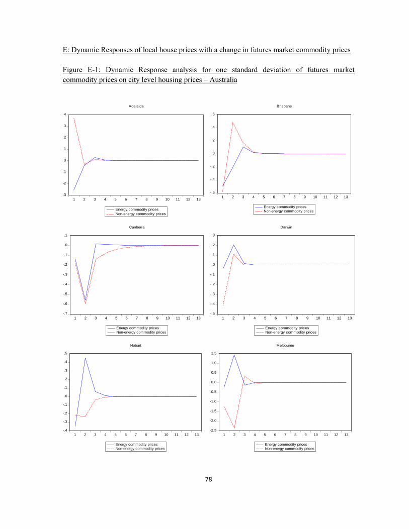
78 

 

E: Dynamic Responses of local house prices with a change in futures market commodity prices Figure E-1: Dynamic Response analysis for one standard deviation of futures market commodity prices on city level housing prices – Australia

-3

-2

-1

0

1

2

3

4

1 2 3 4 5 6 7 8 9 10 11 12 13

Energy commodity pricesNon-energy commodity prices

Adelaide

-.6

-.4

-.2

.0

.2

.4

.6

1 2 3 4 5 6 7 8 9 10 11 12 13

Energy commodity pricesNon-energy commodity prices

Brisbane

-.7

-.6

-.5

-.4

-.3

-.2

-.1

.0

.1

1 2 3 4 5 6 7 8 9 10 11 12 13

Energy commodity pricesNon-energy commodity prices

Canberra

-.5

-.4

-.3

-.2

-.1

.0

.1

.2

.3

1 2 3 4 5 6 7 8 9 10 11 12 13

Energy commodity pricesNon-energy commodity prices

Darwin

-.4

-.3

-.2

-.1

.0

.1

.2

.3

.4

.5

1 2 3 4 5 6 7 8 9 10 11 12 13

Energy commodity pricesNon-energy commodity prices

Hobart

-2.5

-2.0

-1.5

-1.0

-0.5

0.0

0.5

1.0

1.5

1 2 3 4 5 6 7 8 9 10 11 12 13

Energy commodity pricesNon-energy commodity prices

Melbourne

79 

 

-.5

-.4

-.3

-.2

-.1

.0

.1

1 2 3 4 5 6 7 8 9 10 11 12 13

Energy commodity pricesNon-energy commodity prices

Perth

-1.2

-0.8

-0.4

0.0

0.4

0.8

1 2 3 4 5 6 7 8 9 10 11 12 13

Energy commodity pricesNon-energy commodity prices

Sydney

80 

 

Figure E-2: Dynamic Response analysis of futures market commodity prices on selected city level house prices of New Zealand

A few observations follow:

1. For Australian cities, the effects on local house prices from futures market commodity price changes vary significantly across cities. For Brisbane, Canberra, Darwin and Sydney, the effect from energy and non-energy commodity price changes are similar.

2. For New Zealand cities, both energy and non-energy futures market commodity price changes tend to have very similar effect. Initially positive effect of non-energy commodity prices on local house price quickly turns into a negative impact. Overall, the effect on house price quickly dies out.

We admit that at this stage we have not been able to develop very good intuitions for these graphs. Certain data necessary for a more in-depth analysis is missing. We do not have data about the economic structure of different cities. Perhaps equally important, we do not have the home purchase pattern of people in those cities. As we present our paper in different conferences, economists from Australia suggest to us that mine workers, who themselves do not live the major cities, may nevertheless buy their “second houses” in the major cities within the same state for rental income, and thus become literally “absentee landlords”. Media in Australia has provided anecdotal evidence. We are, however, unable to find any systematic evidence for that.

-.4

-.3

-.2

-.1

.0

.1

.2

.3

.4

1 2 3 4 5 6 7 8 9 10 11 12 13

Energy commodity pricesNon-energy commodity prices

Auckland

-.3

-.2

-.1

.0

.1

.2

.3

1 2 3 4 5 6 7 8 9 10 11 12 13

Energy commodity pricesNon-energy commodity prices

Wellington

.0

.1

.2

.3

.4

.5

.6

.7

.8

1 2 3 4 5 6 7 8 9 10 11 12 13

Energy commodity pricesNon-energy commodity prices

Christchurch

81 

 

F. More details of the energy versus non-energy, spot market versus futures market commodity prices   

Some readers are curious why there is a difference in results between spot market commodity prices versus the futures market counterpart. First, we want to recall from the literature that futures market commodity prices do not always predict the subsequent movement in spot market counterparts (e.g. Alquist and Kilian, 2010; Pindyck, 2001; Reichsfeld and Roache, 2011; Sockin and Xiong, 2013, among others). In particular, Sockin and Xiong (2013) show that “…as a result of information frictions, unexpected heavy buying by financial traders can lead to a higher futures price, which, under certain conditions, can in turn drive up producers’ commodity demand and thus the spot price.” Thus, it may be reasonable to expect that the local house price impact of futures market commodity price could be very different from the spot market counterpart. In fact, for the series of both Australia and New Zealand, we calculate the correlation between the spot market commodity price and the futures market counterpart. The correlations are positive and significant. On the other hand, it is also clear that the correlations are less than unity for our sample.  

Correlation (spot market index, futures market index) Australia Energy Commodity Price 0.847*** Australia Non-Energy Commodity Price 0.678*** New Zealand Energy Commodity Price 0.986*** New Zealand Non-Energy Commodity Price 0.811***

  

Key: All series are stationary after first-differencing. *** represents 1% significance level.

In addition, we suspect that one reason why the futures market commodity price may matter more at the national level, while the spot market commodity price matter more at the local level is due to the endogenous government policy. Recently, there are much research efforts on how monetary policy should react to commodity price change (for instance, see Bodenstein et al, 2012; Catao and Chang, 2012; De Gregorio, 2012, among others). And the government (including the central bank and fiscal authority) may have a comparative advantage in responding to changes in the futures market. For instance, the central bank can monitor the futures commodity market prices on a daily basis and may intervene in the money market and/or the foreign exchange market correspondingly. Notice that, unlike small business or households, the central bank in principle has neither a long nor a short position in the commodity market, and hence has no immediate incentive for hedge. Thus, they may be less responsive to the spot commodity prices than the private sector. In addition, we also prove in another section of the appendix that it is not easy to identify the policy effect when the government policies respond to economic variables (including the commodity prices and other macroeconomic variables) endogenously. We can only identify the total effect.

82 

 

Another related question is why the results in Australia and New Zealand are different. Recall that due to the difference in endowment and possibly other historical factors, the composition of commodity export of the two countries are different. Thus, the commodity price series may not be that correlated. The following table enables us to see the difference.

Spot Market Futures Market Corr( energy

AUPC , energyNZPC ) 0.816*** 1.000***

Corr( non energyAUPC , non energy

NZPC ) 0.369** 0.213

Key: All series are stationary after first-differencing. *** and ** represents 1% and 5% significance level respectively.

Clearly, the correlations of energy commodity price series for the two countries are highly correlated, especially in the futures market. On the other hand, for the non-energy commodity price series, the correlations are much weaker. In the case of futures market, the correlation between the two series is not even statistically significant. We speculate that there is at least one more explanation for the discrepancy between the results of spot market commodity prices versus futures market commodity prices. In a standard finance textbook, producers and buyers of commodity would always hedge through the futures market. In practice, we do not know if it is the case. We missed the information of the portfolio of both the commodity producers and buyers. We suspect that there may be a difference between energy commodities versus non-energy commodities. Due to technological or other reasons, energy producers are often large firms, even international firms. On the other hand, non-energy producers may be very large (for instance, in the case of metallic non-energy commodities), and can also be small (for instance, in the case of some farmers who produce food, which are also included as non-energy commodities). Their participation in the spot and futures markets could be different. We regret that we miss the corresponding information and can only leave these speculations to future research.

83 

 

G. An illustration that Tables 4a and 4b are measuring the total effect (This derivation is kindly provided by an anonymous referee, who is gratefully acknowledged by the authors). For expositional purpose, we will assume that there are only two stages of the regression: (and to simplify the exposition, the lags and dynamics are suppressed)

(G1) i ct t t thp P y u

(G2) ct t ty P v

(G1) says that the house price ithp depends on the commodity price c

tP , national economic

variables ty and an innovation term tu . (G2) says that the national economic variables ty may

be affected by the commodity price ctP as well. We can interpret tv as our “commodity price-

filtered economic variables”, or simply “filtered economic variables”. Thus, (G2) is analogous to our first-stage regression. Simply substitute (G2) into (G1) we have

(G3) i ct t t thp P v u

Now (G3) is analogous to our third-stage regression, where the house price is regressed against the commodity price and filtered economic variables. In that case, the corresponding coefficient of the commodity price is the total effect for the commodity price exerting on the house price.

84