Comments on Progress Report n · The Report has been integrated with maps displaying meteo survey station, water level and river discharge survey station and river network. The DTM

MINISTRY OF ENVIRONMENT AND TOURISM Directorate of Integration and Project Coordination

Project ID: P128412 Grant N°: TF 017364

Ref. N°: ESP-CS-QCBS-22

Comments on Progress Report n.1

International Bank for Reconstruction and Development (IBRD) Funds Administrator

February 9th, 2018 Co

nso

rtiu

m

via Guido Rossa 29/A - 35020 Ponte S .Nicolò (Padova) ITALIA

Tel. +39 049 8961120 – Fax +39 049 8961090 - [email protected] – www.betastudio.it

Ministry of Environment and Tourism of Albania

Client

mailto:[email protected]

“CONDUCTING HYDROLOGICAL MODELS AND BATHYMETRIC MEASUREMENTS (Bovilla and Ulza Reservoirs)” BETA Studio s.r.l. – E.B.S Shpk.


I

Document History

0 February 9th, 2018 First release R.Bertaggia A. Pretner S. Fattorelli

REV. DATE NOTE PREPARED VERIFIED APPROVED



1

Comments reply 1. The description of the two watersheds would have been more useful with some interpretation.

What is the implication, for example, of a watershed being ‘mature’?

The hypsometric curve for a drainage basin represents the relative proportion of the watershed are a

below (or above) a given height (Strahler,1952; Schumm, 1956). This surface-elevation curve is a

useful tool for characterising the topographic relief within a drainage basin and, hence, establishing

comparisons between different basins. The shape of the hypsometric curve is related with the stage of

geomorphic development of the basin. Convex hypsometric curves are typical of a youthful stage; s -

shaped curves are related to a maturity stage, and concave curves are indicative of a peneplain stage.

Hypsometric analysis has been widely used in geomorphology, hydrology, and active tectonics.

Figure 1 – (a) Hypsometric curve after Strahler(1952). Area of region under curve (R) is known as hypsometric integral.

Hypsometric curve can be represented by function f(x). Total elevation (H) is relief within basin (maximum elevation

minus the minimum elevation), total area (A) is total surface area of basin, and area (a) is surface area within basin

above a given altitude (h). (b) Changes in hypsometric curves (modified from Ohmori, 1993). Convex curves are typical

for youthful stages of maturity and s-shaped curves and concave curves for mature and old stages. Arrows indicate a

direction of change in curves according to the change in mountain altitude during a geomorphic cycle.



2

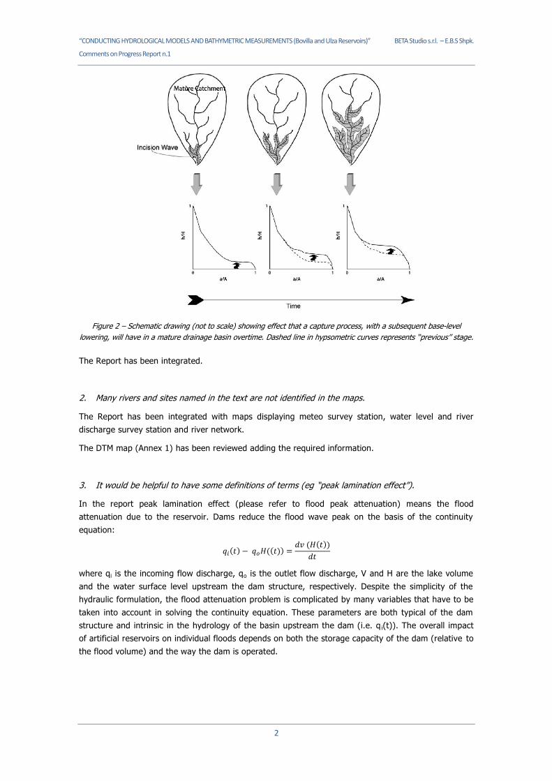
Figure 2 – Schematic drawing (not to scale) showing effect that a capture process, with a subsequent base-level

lowering, will have in a mature drainage basin overtime. Dashed line in hypsometric curves represents ‘‘previous’’ stage.

The Report has been integrated.

2. Many rivers and sites named in the text are not identified in the maps.

The Report has been integrated with maps displaying meteo survey station, water level and river

discharge survey station and river network.

The DTM map (Annex 1) has been reviewed adding the required information.

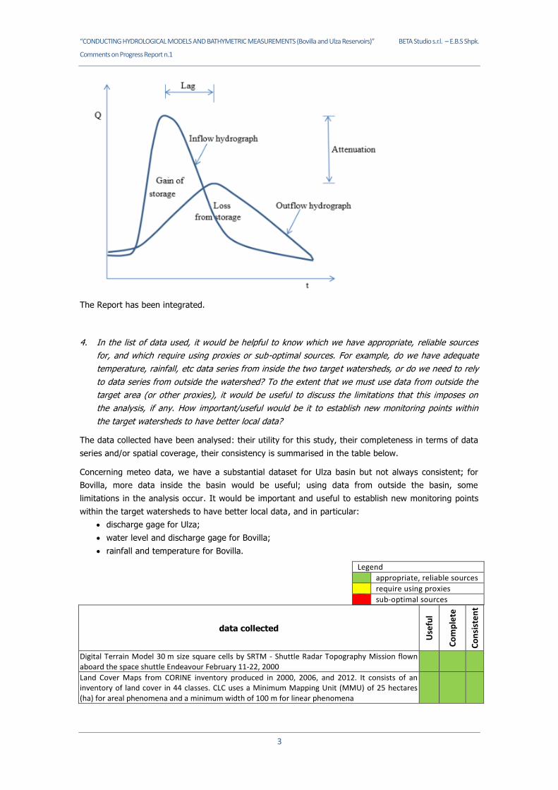
3. It would be helpful to have some definitions of terms (eg “peak lamination effect”).

In the report peak lamination effect (please refer to flood peak attenuation) means the flood

attenuation due to the reservoir. Dams reduce the flood wave peak on the basis of the continuity

equation:

𝑞𝑖(𝑡) − 𝑞𝑜𝐻((𝑡)) =𝑑𝑣 (𝐻(𝑡))

𝑑𝑡

where qi is the incoming flow discharge, qo is the outlet flow discharge, V and H are the lake volume

and the water surface level upstream the dam structure, respectively. Despite the simplicity of the

hydraulic formulation, the flood attenuation problem is complicated by many variables that have to be

taken into account in solving the continuity equation. These parameters are both typical of the dam

structure and intrinsic in the hydrology of the basin upstream the dam (i.e. q i(t)). The overall impact

of artificial reservoirs on individual floods depends on both the storage capacity of the dam (relative to

the flood volume) and the way the dam is operated.



3


4. In the list of data used, it would be helpful to know which we have appropriate, reliable sources

for, and which require using proxies or sub-optimal sources. For example, do we have adequate

temperature, rainfall, etc data series from inside the two target watersheds, or do we need to rely

to data series from outside the watershed? To the extent that we must use data from outside the

target area (or other proxies), it would be useful to discuss the limitations that this imposes on

the analysis, if any. How important/useful would be it to establish new monitoring points within

the target watersheds to have better local data?

The data collected have been analysed: their utility for this study, their completeness in terms of data

series and/or spatial coverage, their consistency is summarised in the table below.

Concerning meteo data, we have a substantial dataset for Ulza basin but not always consistent; for

Bovilla, more data inside the basin would be useful; using data from outside the basin, some

limitations in the analysis occur. It would be important and useful to establish new monitoring points

within the target watersheds to have better local data, and in particular:

discharge gage for Ulza;

water level and discharge gage for Bovilla;

rainfall and temperature for Bovilla.

Legend

appropriate, reliable sources

require using proxies

sub-optimal sources

data collected

Use

ful

Co

mp

lete

Co

nsi

ste

nt

Digital Terrain Model 30 m size square cells by SRTM - Shuttle Radar Topography Mission flown aboard the space shuttle Endeavour February 11-22, 2000

Land Cover Maps from CORINE inventory produced in 2000, 2006, and 2012. It consists of an inventory of land cover in 44 classes. CLC uses a Minimum Mapping Unit (MMU) of 25 hectares (ha) for areal phenomena and a minimum width of 100 m for linear phenomena



4

data collected

Use

ful

Co

mp

lete

Co

nsi

ste

nt

Land Cover Map for Bovilla watershed edited in 2017 by the Ministry of Environment and Tourism GIS Office

River networks from EU-Hydro Drainage Database that is a photo-interpreted river network for EEA39 derived from satellite imagery supplemented with ancillary data sources

River sections topographic survey River watersheds from EU-Hydro River network dataset consistent of surface interpretation of water bodies (lakes and wide rivers), and a drainage model (also called Drainage Network), derived from EU-DEM, with catchments and drainage lines and nodes

2007 Ortophoto Tree cover density map and Forest type map derived by semi-automatic classification and computer aided visual refinement, based on ESA provided HR satellite imagery (DWH_M62_CORE_01) with additional EO data for the area of the EEA39) and subsequently final integration to a European mosaic

International Geological Map of Europe (www.europe-geology.eu) International Hydrogeological Map of Europe BGR & UNESCO (eds.) (2014) (www.europe-geology.eu). It consists of selected issues of the IHME1500 with the following content

Aquifer types (area): Distinction of six types of aquifers according to their productivity und rock types

Lithology (area): Lithological classification of the aquifers at five aggregation levels Siltation: sediment transport analysis data (including grain size) Seawater intrusion (area): Areas with salination of groundwater caused by sea water intrusion Tectonic fractures (line): Geological lineaments assigned to the five classes of known or supposed faults or overthrusts and boundaries of fractured belts in Iceland

Soil regions, Soil type and Soil texture maps from PROGETTO INTERREG II ITALIA-ALBANIA - Sistemi Informativi sui Suoli (SIS) della Repubblica d’Albania

2013 Ulza Bathymetric survey by CNVP Foundation for WB-PROFOR “Study and Analysis of Innovative Financing for Sustainable Forest Management in the Southwest Balkan”

Rainfall Tirana (from 2002 to 2011) Rainfall Klos (from 2002 to 2011) Rainfall Burrell (from 2002 to 2011) Rainfall Bulqize (from 2002 to 2011) Rainfall Kurbnesh (from 2002 to 2011) Rainfall Dajt (from 2002 to 2011) Rainfall Linze (from 2002 to 2011) Rainfall Shengjergj (from 2002 to 2011) Rainfall Zallmner (from 1960 to 1990) Temperature Tirana (from 2002 to 2011) Temperature Burrell (from 2002 to 2011) Temperature Kurbnesh (from 2002 to 2011) Temperature Dajt (from 2002 to 2011) Temperature Linze (from 2002 to 2011) Temperature Shengjergj (from 2002 to 2011) Temperature Kruje (from 1960 to 1990) Daily average wind speed at the station of Burrell (from 2004 to 2011) Daily average relative humidity at the station of Tirana (from 2002 to 2011) Daily average water level at the discharge survey station of Shoshaj on Mati river from 1998 to 2008

Daily average discharge from and water level in Ulza reservoir from 1959 to June 2017 Daily average water level in Bovilla reservoir from 2002 to 2008



5

5. A brief discussion/explanation of the reasons for the choice of the specific model to be used would

be helpful – including a brief summary of the strengths and weaknesses of the chosen model,

citations to other applications, any caveats that should be borne in mind when interpreting results.

The Hydrologic Modeling System (HEC-HMS) is one of the most widely used simulation tools developed

by the U. S. Army Corps of Engineers Hydrologic Engineering Center (HEC), and is designed to

simulate the rainfall-runoff processes of dendritic drainage basin. A soil moisture accounting (SMA)

algorithm has been used to evaluate the performance of the HEC-HMS model for many river basins.

The software includes many traditional hydrologic analysis procedures such as event infiltration, unit

hydrographs, and hydrologic routing. HEC-HMS also includes procedures necessary for continuous

simulation including evapo-transpiration, snowmelt, and soil moisture accounting. Advanced

capabilities are also provided for gridded runoff simulation using the linear quasi-distributed runoff

transform (ModClark). Supplemental analysis tools are provided for model optimization, forecasting

streamflow, depth-area reduction, assessing model uncertainty, erosion and sediment transport, and

water quality.

The software features a completely integrated work environment including a database, data entry

utilities, computation engine, and results reporting tools. A graphical user interface allows the user

seamless movement between the different parts of the software. Simulation results are stored in HEC-

DSS (Data Storage System) and can be used in conjunction with other software for studies of water

availability, urban drainage, flow forecasting, future urbanization impact, reservoir spillway design,

flood damage reduction, floodplain regulation, and systems operation.

Besides the experience gathered by the JV, a lot of application report are presented on the

Softwarehouse web site :http://www.hec.usace.army.mil/publications/

The Report has been integrated with some example.

6. The detailed explanation of how the model works could be moved to an annex.

Done.

7. To what extent are the parameters in Table 4.2 approximations used in the absence of better

data? Are the model results particularly sensitive to certain parameters?

In absence of measured data, the parameters’ values of the hydrological model were assigned on the

basis of acceptable data ranges from the manual, from literature and on the Consultants’ experience.

The parameters have been finalised in order to well match the simulated and observed data (runoff

and yearly amount of sediment).

The variables and their ranges are described below.

Canopy storage represents the maximum amount of water that can be held on leaves before through-

fall to the surface begins and is specified as an effective depth of water. This was assigned by

manual’s range, equal to 4 mm.

Surface storage represents the maximum amount of water that can be held on the soil surface before

surface runoff begins and is specified as an effective depth of water. This was assigned by manual’s

range, equal to 2 mm.

Both previous parameters affect the losses and the delay between the rain and the runoff.

For each subbasin the lag time was computed as 0.6 the time of concentration, and depends on

http://www.hec.usace.army.mil/publications/



6

morphological factors.

The soil moisture accounting loss method uses three layers (soil, groundwater 1 and groundwater

2) to represent the dynamics of water movement in the soil and should be used with the canopy and

surface methods. The soil layer will dry out between precipitation events as the canopy extracts soil

water. The surface layer holds precipitation and allows it to infiltrate after the rain has stopped.

Infiltration is generally reduced if no surface method is selected. The soil layer is subdivided into

tension storage and gravity storage. Groundwater layers are not designed to represent aquifer

processes but are used for representing shallow interflow processes.

The initial condition of the soil is specified as the percentage of the soil that is full of water at the

beginning of the simulation. It was assigned equal to 85% from calibration. It affects only the very

first period of the simulation.

The maximum infiltration rate sets the upper bound on infiltration from the surface storage into the

soil: it has been set equal to 10 mm/hr (sandy loamy soils). The percentage of the subbasin which is

subject to direct runoff (Impervious) was assigned equal to 30% from calibration.

Soil storage represents the total storage available in the soil layer. Tension storage specifies the

amount of water storage in the soil that does not drain under the effects of gravity. Percolation from

the soil layer will occur whenever the current soil storage exceeds the tension storage. Water in

tension storage is only removed by evapotranspiration. By definition tension storage must be less than

soil storage. The soil percolation sets the upper bound on percolation from the soil storage into the

upper groundwater. Groundwater 1 storage represents the total storage in the upper groundwater

layer. The groundwater 1 percolation rate sets the upper bound on percolation from the upper

groundwater to the lower groundwater. The groundwater 1 coefficient is used as the time lag on a

linear reservoir for transforming water in storage to become lateral outflow. The lateral outflow is

available to become base flow. Similarly for Groundwater layer 2, not used in this model. Parameters

have been set based on manual’s range and calibration results.

The MUSLE method was adapted from the original Universal Soil Loss Equation. The original equation

was based on precipitation intensity, and could not differentiate between storms with low or high

infiltration. With high infiltration, there is little surface runoff and little accompanying surface erosion.

Conversely, low infiltration events have relatively more surface runoff and more surface erosion. The

modifications to the original USLE equation changed the formulation to calculate erosion from surface

runoff instead of precipitation. The method works best in agricultural environments where it was

developed.

The erodibility factor describes the difficulty of eroding the soil. The factor is a function of the soil

texture, structure, organic matter content and permeability. Typical range from 0.05 for

unconsolidated loamy sand to 0.75 for silty and clayey loam soils. In the model 0.1 has been adopted

according to calibration on available siltation data.

The topographic factor describes the susceptibility to erosion due to length and slope. It is based on

the observation that long slopes have more erosion than short slopes, and steep slopes have more

erosion than flat slopes. Typical values range from 0.1 for short and flat slopes to 10 for long or steep

slopes. In the model 0.1 and 0.3 values have been adopted, on the basis of subbasin’s slope.

The cover factor describes the influence of plant cover on surface erosion. Bare ground in the most

susceptible to erosion while a thick vegetation cover significantly reduces erosion. Typical values range

from 1.0 for bare ground to 0.1 for fully mulched or covered soils, to as small as 0.0001 for forest soils

with a well-developed soil O horizon under a dense tree canopy. In the model 0.001 and 0.002 values

have been adopted, on the basis of ortophoto’s analysis.



7

The practice factor describes the effect of specific soil conservation practices, sometimes called best

management practices. Agricultural practices could include strip cropping, terracing or contouring.

Construction and urban practices could include silt fences, hydro seeding and settling basins. It is

difficult to establish general ranges, because highly specific.

Only some precipitation events will cause surface erosion. The threshold can be used to set the lower

limit for runoff events that cause erosion. This parameter has been set to 3 m³/s.

Based on experience and calibration phase, the more sensitive parameters are: maximum infiltration

rate, soil storage (for runoff), erodibility factor and cover factor (for soil erosion).

The research article by Jang Pak et al. (2015) Sensitivity analysis for sediment transport in the

Hydrologic Modeling System (HEC-HMS) confirms that the more sensitive parameters in these kind of

calculations are the MUSLE cover factor and the grain-size of sediment.

8. The model seems to have a generally good fit to observed data, but it does not seem to predict

the peak inflows very well. That would seem to be a problem if we were trying to predict flood

risk. But is it likely to affect predictions of sediment delivery to the reservoir?

The study aim is the evaluation of average sediment delivery and seasonal water balance. For this

purpose the model shows a very good fit to observed data.

The flood risk prediction isn’t the aim of the project. For this kind of study a different model setting

and kind of data are needed: must be available and used hourly (not daily average) rain and discharge

data.

9. Is there any reason why the Bovilla results are presented in a different way than those for Ulza

(no equivalent to figures 4.9-4.13 for Bovilla)?

For Bovilla any discharge gauged data set is available. The model can’t be calibrated without this kind

of data, so it’s been implemented extending Ulza’s parameters except for the morphological ones (time

lag, slopes etc).

10. Are we correct in interpreting the discussion at the bottom of p.41 to imply that the transect

spacing is well below the recommended level? Or is this discussion indicating a problem that was

addressed? If so, that is not clear from the report. Please clarify.

Yes you are. Much more points than the minimum suggested by literature have been collected to have

a survey as much detailed and accurate as possible. The Report has been integrated.

11. Is the measured sediment captured in the reservoir (ca 2 million m3 in 21 years) consistent with

the estimated sediment delivery from the model and the estimated capture efficiency? (and,

likewise, is estimated sediment delivery at Ulza consistent with the results of the bathymetric

measurements conducted there a few years ago?)

An evaluation of sediment delivery for Bovilla basin with the Hydrological model has not been

performed yet because it will be a task to be developed, according to TOR, on the 2^ Progress Report.

Total specific average annual sediment inflow measured for Bovilla (1’333 t/y,km²), however, is

consistent with the estimation from the model applied to Ulza (1’269 t/y,km²) and the bathymetric

measurements conducted there a few years ago (1’390 t/y,km², source PROFOR-WB).



8


12. p.55 – what is the parameter Sa = 95,723 used in the lifespan calculation? Is it the 2 million m3

of sediment captured in the reservoir, divided by the 21 years of reservoir li fe so far (that is,

average annual sediment captured in the reservoir)?

Yes it is. The Report has been integrated.

13. The lifespan formula on p.55 tells us how much time it will take until the reservoir is completely

filled with sediment. But surely problems will begin much sooner: (1) as capacity declines, the

ability to store water will decline; a greater fraction of inflows will be spilled, a smaller fraction will

be available for use in dry periods; (2) the reservoir will actually become unusable when the

accumulated silt near the water intake reaches the level of the water intake. Figure 2.5 seems to

show a series of three intakes, at different levels. Is that correct? If we are interpreting this

correctly, the lowest intake becomes unusable once accumulated silt reached levels 275, then the

second when it reaches level 284, and the third when it reaches level 290 or so. Is that correct?

Does water treatment at Bovilla require all three intakes to be operable, or is one sufficient? Is

there a reduction in the volume that can be used, for example, if some of the intakes are not

operable?

The Report contains some very preliminary evaluation on the lifespan analysis. The above question will

be addressed in the following tasks of the project.

14. Is it possible to flush out sediment accumulated near the intakes by opening the large spill gate?

Question should be addressed to Authority in charge for the operation of the dam. If the Authority

provide us with dam details (drawings and data), we might provide some evaluation.

15. If the reasoning that silt reaching the level of the intakes causes problems is correct, is it possible

to estimate from current data how soon that will happen?

See comment 13.

16. Section 6.2 — Have you examined the data being generated from the erosion monitoring plots in

Ulza and Bovilla watersheds? It should allow estimation of erodibility factors and soil cover and

practice factors for the main land uses.

Please, clarify your question.

Documents

Comments on Progress Report n · The Report has been integrated with maps displaying meteo survey station, water level and river discharge survey station and river network. The DTM