Commentary on the DSP First Labsweb.mit.edu/jrising/Public/dsplabs.pdf · Commentary on the DSP First Labs, In which is discussed the concerns of such labs as might be found in the

Commentary on the DSP First Labs,In which is discussed the concerns of such labs as might

be found in the book of record, in addition to

supplemental work suitable for a college class on these

topics.

Jimmy Rising∗

July 12, 2005

∗This document reflects the labs taught in Signals and Systems at Olin College during Fall 2003 andSpring 2004, under Dr. Diana Dabby.

1

Contents

1 Preface 6

1.1 Document Format . . . . . . . . . . . . . . . . 6

1.1.1 Typefaces . . . . . . . . . . . . . . . . . 7

1.2 Past Lab Policies . . . . . . . . . . . . . . . . . 7

1.2.1 Deliverables . . . . . . . . . . . . . . . . 7

1.2.2 Collaboration . . . . . . . . . . . . . . . 8

1.3 Example Syllabus . . . . . . . . . . . . . . . . . 8

1.4 Future Work . . . . . . . . . . . . . . . . . . . 9

2 General Notes 10

2.1 The CD . . . . . . . . . . . . . . . . . . . . . . 10

2.2 Book Notation . . . . . . . . . . . . . . . . . . 10

3 Lab 1: Introduction to Matlab 10

3.1 Introduction . . . . . . . . . . . . . . . . . . . . 11

3.1.1 Installing DSPFirst . . . . . . . . . . . 11

3.1.2 Measuring Phases . . . . . . . . . . . . 12

3.2 Additional Notes . . . . . . . . . . . . . . . . . 12

3.2.1 Question Help . . . . . . . . . . . . . . 12

3.2.2 Section Commentary . . . . . . . . . . . 13

3.3 Deliverables . . . . . . . . . . . . . . . . . . . . 13

3.3.1 Grading . . . . . . . . . . . . . . . . . . 13

4 Lab 2: Introduction to Complex Exponentials 15

4.1 Introduction . . . . . . . . . . . . . . . . . . . . 15

4.1.1 Fixing zvect and zcat . . . . . . . . . . 15

4.1.2 Explaining sumcos . . . . . . . . . . . . 15


4.2.1 Student Supplement . . . . . . . . . . . 17

4.3 Deliverables . . . . . . . . . . . . . . . . . . . . 18

4.3.1 Grading . . . . . . . . . . . . . . . . . . 18

5 Lab 3: Synthesis of Sinusoidal Signals 20

5.1 Introduction . . . . . . . . . . . . . . . . . . . . 20

5.1.1 Minimal Music Theory . . . . . . . . . . 21

5.1.2 Harmonics and Other Improvements . . 21


5.2.1 Student Supplement . . . . . . . . . . . 22

5.2.2 Question Help . . . . . . . . . . . . . . 23

5.3 Deliverables . . . . . . . . . . . . . . . . . . . . 23

5.3.1 Grading . . . . . . . . . . . . . . . . . . 24

6 Lab 4: AM and FM Sinusoidal Signals 25

6.1 Introduction . . . . . . . . . . . . . . . . . . . . 25

6.1.1 Instantaneous Frequency . . . . . . . . . 25

6.1.2 Reading Spectrograms . . . . . . . . . . 25



6.3 Deliverables . . . . . . . . . . . . . . . . . . . . 27

6.3.1 Grading . . . . . . . . . . . . . . . . . . 27

7 Lab S: Sampling and Aliasing 29

7.1 Introduction . . . . . . . . . . . . . . . . . . . . 29

7.1.1 Tone Shifting System . . . . . . . . . . 29


7.2.1 Question Help . . . . . . . . . . . . . . 30

7.3 Deliverables . . . . . . . . . . . . . . . . . . . . 30

7.3.1 Grading . . . . . . . . . . . . . . . . . . 30

2

8 Lab C: Convolution Lab 35

8.1 Introduction . . . . . . . . . . . . . . . . . . . . 35


8.3 Deliverables . . . . . . . . . . . . . . . . . . . . 37

8.3.1 Grading . . . . . . . . . . . . . . . . . . 37

9 Lab 5: FIR Filtering of Sinusoidal Waveforms 37

9.1 Introduction . . . . . . . . . . . . . . . . . . . . 37

9.2 Deliverables . . . . . . . . . . . . . . . . . . . . 38

9.2.1 Grading . . . . . . . . . . . . . . . . . . 38

10 Lab 6: Filtering of Sampled Waveforms: Cas-cading Systems 40

10.1 Introduction . . . . . . . . . . . . . . . . . . . . 41


10.2.1 Question Help . . . . . . . . . . . . . . 41

10.3 Deliverables . . . . . . . . . . . . . . . . . . . . 41

10.3.1 Grading . . . . . . . . . . . . . . . . . . 41

11 Lab 6: Filtering of Sampled Waveforms: Filter-ing the Speech Waveform 44

11.1 Introduction . . . . . . . . . . . . . . . . . . . . 44


11.2.1 Question Help . . . . . . . . . . . . . . 45

11.3 Deliverables . . . . . . . . . . . . . . . . . . . . 45

11.3.1 Grading . . . . . . . . . . . . . . . . . . 45

12 Lab 7: Everyday Sinusoidal Signals: TelephoneTouch Tone Dialing 49

12.1 Introduction . . . . . . . . . . . . . . . . . . . . 49

12.1.1 Detecting Energy . . . . . . . . . . . . . 49


12.2.1 Question Help . . . . . . . . . . . . . . 50


12.3 Deliverables . . . . . . . . . . . . . . . . . . . . 50

12.3.1 Grading . . . . . . . . . . . . . . . . . . 50

13 Lab 7: Everyday Sinusoidal Signals: Tone Am-plitude Modulation 53

13.1 Introduction . . . . . . . . . . . . . . . . . . . . 53


13.3 Deliverables . . . . . . . . . . . . . . . . . . . . 54

13.3.1 Grading . . . . . . . . . . . . . . . . . . 54

14 Lab 8: Filtering and Edge Detection of Images 56

14.1 Introduction . . . . . . . . . . . . . . . . . . . . 57

14.1.1 Mechanics of show img . . . . . . . . . . 57

14.1.2 Applying Filters to Images . . . . . . . 58

14.1.3 Understanding Image Frequency Content 58


14.2.1 Question Help . . . . . . . . . . . . . . 59

14.3 Deliverables . . . . . . . . . . . . . . . . . . . . 59

14.3.1 Grading . . . . . . . . . . . . . . . . . . 60

15 Lab 9: Sampling and Zooming of Images 65

15.1 Introduction . . . . . . . . . . . . . . . . . . . . 65


15.2.1 Question Help . . . . . . . . . . . . . . 66

15.3 Deliverables . . . . . . . . . . . . . . . . . . . . 67

15.3.1 Grading . . . . . . . . . . . . . . . . . . 67

16 Lab 10: The z−, n−, and ω−Domains 70

16.1 Introduction . . . . . . . . . . . . . . . . . . . . 70


3

16.3 Deliverables . . . . . . . . . . . . . . . . . . . . 71

16.3.1 Grading . . . . . . . . . . . . . . . . . . 71

17 Lab 11: Extracting Frequencies of MusicalTones 71

17.1 Introduction . . . . . . . . . . . . . . . . . . . . 72

17.1.1 Question Help . . . . . . . . . . . . . . 72

17.2 Deliverables . . . . . . . . . . . . . . . . . . . . 72

17.2.1 Grading . . . . . . . . . . . . . . . . . . 72

A Frequently Asked Questions 73

B Matlab Function Notes 74

B.1 Freqz . . . . . . . . . . . . . . . . . . . . . . . . 74

B.2 Specgram . . . . . . . . . . . . . . . . . . . . . 75

B.3 Hist . . . . . . . . . . . . . . . . . . . . . . . . 75

B.4 Wavread . . . . . . . . . . . . . . . . . . . . . . 76

B.5 Wavwrite . . . . . . . . . . . . . . . . . . . . . 76

C Other Exercises and Demonstrations 76

C.1 Sound Demos . . . . . . . . . . . . . . . . . . . 76

C.2 Convolution Theater . . . . . . . . . . . . . . . 77

C.2.1 Graphical Convolution Method . . . . . 77

C.2.2 System Processing Method . . . . . . . 77

D Your Everyday Sinusoid 79

E Independent Project Proposal 81

F Lab S: Sampling and Aliasing 83

F.1 Simple Examples . . . . . . . . . . . . . . . . . 83

F.1.1 Chirp Folding . . . . . . . . . . . . . . . 83

F.1.2 Sinusoid Sampling . . . . . . . . . . . . 83

F.1.3 Folding in Music . . . . . . . . . . . . . 83

F.2 Adjusting Pitch . . . . . . . . . . . . . . . . . . 84

G Lab C: Convolution Lab 87

G.1 Short Discussion of Calculating Convolutions . 87

G.1.1 Using the Impulse Response . . . . . . . 87

G.1.2 Using the “Graphical Method” . . . . . 88

G.2 Block Diagrams . . . . . . . . . . . . . . . . . . 88

G.2.1 Basic Add and Multiply Blocks . . . . . 89

G.2.2 The Delay Block . . . . . . . . . . . . . 89

G.2.3 Improving the Blocks . . . . . . . . . . 89

G.2.4 Creating Systems . . . . . . . . . . . . . 90

G.2.5 Making the Demos . . . . . . . . . . . . 90

G.3 Demo Sound-track . . . . . . . . . . . . . . . . 91

G.3.1 Loading Music . . . . . . . . . . . . . . 91

G.3.2 Note-Pass Filter . . . . . . . . . . . . . 91

G.4 Final Notes . . . . . . . . . . . . . . . . . . . . 93

H Image Magnitude and Phase Supplement 94

I Lab 11: Extracting Frequencies of MusicalTones 96

I.1 Note Filters . . . . . . . . . . . . . . . . . . . . 96

J Matlab Primer by Brian Storey 98

J.1 Getting Started . . . . . . . . . . . . . . . . . . 99

J.2 Calculator . . . . . . . . . . . . . . . . . . . . . 99

J.3 Variables . . . . . . . . . . . . . . . . . . . . . 101

J.4 One-dimensional arrays . . . . . . . . . . . . . 103

J.5 Plotting . . . . . . . . . . . . . . . . . . . . . . 108

J.6 Two-dimensional arrays . . . . . . . . . . . . . 110

4

J.7 Relational operators . . . . . . . . . . . . . . . 113

J.8 Scripts . . . . . . . . . . . . . . . . . . . . . . . 116

J.9 Control flow . . . . . . . . . . . . . . . . . . . . 116

J.10 Logical Operators . . . . . . . . . . . . . . . . . 121

J.11 Files . . . . . . . . . . . . . . . . . . . . . . . . 121

J.12 Example: Numerical Integration . . . . . . . . 123

J.13 Example: Rate Equations . . . . . . . . . . . . 125

J.14 Example: Plotting Experimental Data . . . . . 127

J.15 Functions . . . . . . . . . . . . . . . . . . . . . 130

J.16 Problems . . . . . . . . . . . . . . . . . . . . . 137

5

1 Preface

This document is intended to supplement the Matlab labs included in DSPFirst1for usein a class on Signals and Systems. It includes the clarifications, corrections, and lecturenotes (’class-ifications’) that we found to be necessary, and occasionally helpful. The noteshere are generally not intended to replace the lab descriptions in DSPFirst, and should beused in combination with them. This commentary is based on the experiences from the labsand class taught by Jimmy and Diana, respectively, during Fall 2003 and Spring 2004. Wehoped to save these thoughts for future generations of students.

1.1 Document Format

This document is organized around each DSPFirstlab and class activity. A subset of thesewere presented, in order, throughout each semester. A sample syllabus is included at theend of this section.

Each lab is divided into three sections.

Introduction : The lab introduction maps to my discussion of each lab before setting thestudents loose to work on it during the lab time. It variously includes content delivery,explanations, and warnings.

Additional Notes : This section might include several different topics: “Student Sup-plement” sections to be made available to the students directly; “Question Help”concerning how to help students through common problems; and “Section Commen-tary”, with notes and clarifications on the labs on a section-by-section basis.

Deliverables : This describes what should be turned in for evaluation. In the instructor’sversion of this document, this section includes a part on Grading, with notes on whatto look for and how to respond.

1

DSP First: A Multimedia Approach by James H. McClellan, Ronald W. Schafer,and Mark A. Yoder (Prentice Hall, 1997), ISBN 0132431718

6

1.1.1 Typefaces

Different typefaces are used to denote the use and audience of the comments.

• Roman font: These are comments for the instructor.

• Sans serif: These comments are directed toward students.

• Monospace font: Matlab commands and computer or programming text.

• Italics: These are thoughts or untested suggestions.

The comments to students and methods of teaching are meant to be suggestions and a recordfor how I teach. Even as that, they are incomplete and reflect broad strokes more than actualverbiage. If they do not work for you, do not use them.

1.2 Past Lab Policies

Every week, a two-hour block was set aside for in-class lab. I would use the first 15 to 40minutes of this time to handle general class business, get feedback from students on recenthappenings, introduce the lab and teach any important topics related to it. The rest of thetime was available for students to work and ask questions. If there were too many questionsto answer, I would start a question queue on the board and invite students to add theirnames to the end.

Each lab would be due 112

weeks later. Students would place the deliverables for each lab in afolder on Olin’s StuFac server (stufps01/stufac/Signals and Systems/Lab Turnins/<Student>/<Lab>

and then email me. I would work through the emails in order. I do not use the InstructorVerification Sheets from DSPFirst.

I do use repetitive grading. Students could turn in labs as many times as they wished upto the due date, but did not get much credit for incorrect or incomplete work. When I wasbehind on grading, as I often was, I would specify in my emailed reply how many days theyhad remaining from that point to do corrections, discounting all but one of the days theyhad to wait for the feedback.

1.2.1 Deliverables

My interest is in the doing of things, not the writing-up of them. What I expect in lab reports,

7

then, is exactly as much information as I need to see that you did the exercise and understood it.In general, that means including, succinctly, what you did for the lab (often Matlab code) andwhat you got for results (often graphs). For every lab, turn in a folder with all of your files (onStuFac), plus an index file which tells me what the other files are, as well as your collaboratorsand time-spent. You may make a single document with your comments, code, and graphs, orinclude your graphs and code in separate files in the same directory, as specified by your indexfile. If you wrote an m-file for the lab, include it in your folder; if you just wrote commands intoMatlab’s window, you can just copy those lines into your index file.

Irregular reminders to include time-spent and collaborators in lab reports are useful.

1.2.2 Collaboration

Your labs should be your own work. Feel free to work together (e.g., side-by-side, discussing theproblems), but don’t explicitly share your solutions.

1.3 Example Syllabus

As a way to gauge the semester as a whole, here is a sample syllabus, which reflects a currentsense of the “best practice”. Each actual syllabus will deviate as needed for the structure ofthe semester and for new ideas.

8

Week Class Topics Lab Introduced and BusinessWeek 1 Appendix A: Complex Numbers

Appendix A Lab 1: Introduction to MatlabWeek 2 Chapter 2: Sinusoids

Chapter 2 Lab 2: Introduction to Complex ExponentialsWeek 3 Chapter 3: Spectrum Representation Lab 1 Due

Chapter 3 Lab 3: Synthesis of Sinusoidal SignalsWeek 4 Chapter 3 Lab 2 Due

Chapter 4: Sampling and Aliasing Lab 3 ContinuedWeek 5 Chapter 4

Chapter 4 Lab 4: AM and FM Sinusoidal WaveformsWeek 6 Exam 1 Lab 3 Due

Chapter 5: FIR Filters Lab S: Sampling and AliasingWeek 7 Chapter 5 Lab 4 Due

Chapter 5 Lab 5: FIR Filtering of Sinusoidal SignalsWeek 8 Chapter 6: Frequency Response of FIR Filters Lab S Due

Chapter 6 Lab 6: Filtering Sampled Waveforms (either)Week 9 Chapter 6 Lab 5 Due

Chapter 7: z-Transforms Lab 7: Everyday Sinusoidal Signals (either)Week 10 Chapter 7 Lab 6 Due

Chapter 7 Lab 8: Filtering and Edge Detection of Images and supplementWeek 11 Chapter 8: IIR Filters Lab 7 Due

Exam 2 Lab 9: Sampling and Zooming of ImagesWeek 12 Chapter 8 Lab 8 Due

Chapter 8 Individual Projects and Lab 10: The z-, n-, and ω-DomainsWeek 13 Chapter 9: Spectrum Analysis Lab 9 Due

Chapter 9 Projects and Lab 11: Extracting Frequencies of Musical TonesWeek 14 Chapter 9 Lab 10 Due

Chapter 9 Lab 11 Due; Individual Projects Due

Although the following are described below, I have not included them in the sample syllabus.

• Everyday Sinusoids: While this assignment got interesting responses, it is ultimatelynot yet well enough integrated into the course.

• Lab C: This lab is a bit too advanced for the place in the semester for which it waswritten, and the material is put to better use as a replacement for lab 11.

Note that the current replacement for lab 11 uses the same methodology as Lab 7: TelephoneTouch-tone Dialing. If you choose the telephone lab, you may want to do lab 11 differently.

1.4 Future Work

There remain some holes to be filled in this class, and in this document:

New Convolution Lab : A replacement for Lab C with simple, intuitive exercises tounderstand convolution and its methods of calculation.

More Demonstrations : Additional demonstrations were used in the class, and it wouldbenefit greatly from even more.

9

2 General Notes

2.1 The CD

There are small differences between material as it appears in the book and on the CD. Forexample, in the labs the section numbers are different between the book and the CD. Thenumbers used below are from the book.

In the grading and section-by-section comments, each number refers to a specific book orlab section, as shown below:

C.1.3.1:Manipulating Sinusoids with Matlab :

1. This refers to C.1.3.1.1

2.2 Book Notation

Matlab matrix indices start at 1, while the book consistently starts indices for finitediscrete-time functions with n = 0. As a result, the following are equivalent: h[0], h0,and hh(1). Generally, for discrete-time functions, the book will use the index n, for FIRfilters it uses the subscript k, and for Matlab vectors, in cases where indices cannot beavoided, nn or ii. This can cause confusion, as n = k = nn −1.

3 Lab 1: Introduction to Matlab

Ingredients: C.1.2.2: Matlab Array Indexing, C.1.2.5: Matlab Sound,C.1.2.7: Vectorization, DSPFirst CD

Indications: before other Matlab workWarnings: noneDirections: see belowLast Used: Fall 2003, Spring 2004

10

3.1 Introduction

I begin with introductions (myself and the role of labs in the class). This is the time I use todiscuss lab policies, the use of the questions queue, and lab report expectations, as describedabove.

Appendix B of DSPFirst is a wonderful introduction to Matlab. Brian Storey has writtenan even better introduction to Matlab in general, although it is less specifically applicableto our work. The largest time sink students experience in this class is from struggling withMatlab commands. Use help liberally, but if you are struggling with a feature of Matlab,ask for help before you get frustrated!

As soon as possible, find out how well each student knows Matlab and set up tutorialsfor those who need them. This might be done in the same questionnaire that asks for aself-assessment of each student’s competencies or an early feedback survey.

Now help everyone install the DSPFirst functions (see 3.1.1 below).

Demo zdrill. In class, you’ve been working with complex numbers. zdrill may be helpful foryou to improve your understanding of them, though we’re not going to use it directly.

Explain the format of the book labs (introduction/background, warm-ups, and exercises),and that they do not have to do the warm-ups unless specified, but might find them useful.

The first lab is comprised of exercises in Matlab. If you are comfortable with Matlab, theexercises should take very little time.

3.1.1 Installing DSPFirst

Have some network cables for those who do not have their books.

1. Copy dspfirst.exe from the CD (MATLAB\WINDOWS\DSPFIRST.EXE) or StuFac (stufps01/stufac/Signalsand Systems/DSPFirst/MATLAB/WINDOWS/DSPFIRST.EXE) and place it in your Mat-

lab toolbox directory (C:\MATLAB...\toolbox).

2. Run dspfirst.exe. It will open a window and extract its contents (a DSPFIRST

directory) to your toolbox.

3. Open Matlab.

11

4. From the File menu, select Add Path.... Click Add with subfolders and browseto the new DSPFIRST directory. Select it and click okay. Your path list will be updatedwith the subdirectories of DSPFIRST. Then click Save.

Spend time this week familiarizing yourself with the CD, which has many goodies and the website,which might too.

3.1.2 Measuring Phases

There are two common ways to measure the phase of a sinusoid from a graph. You may use anymethod you wish, but your answer should be correct to at least 2 significant figures.

The first method is the most intuitive. Draw a sinusoid with coordinate axes and a peak leftof the origin. Start by measuring the period (mark the x-coordinate of two peaks). Now,imagine, then if this were an unshifted cosine wave, its first peak would be at 0. Intuitively, then,the fraction of this first peak location (indicate the peak closest to zero) to the total period,times 2π is the phase shift. Remember to adjust the sign of the phase shift: left is positive, rightis negative. In other words, the relation between time shift and phase shift is − t0

T= φ

2π, where

t0 is the peak location, T is the period, and φ is the phase shift.

The second method is more analytic, and more precise, if you know the value at 0. The equationfor a sinusoid is x(t) = Acos(ωt + φ). Evaluate this at t = 0 and rearrange to get x(0)

A= cos(φ)

or φ = cos−1(x(0)A

). In other words, if you measure the y-intercept, which you can usually doprecisely with Matlab, divide by the amplitude, and take the inverse cosine, you get the phaseshift. The result will always be positive, so you still have to add on the sign.

3.2 Additional Notes

3.2.1 Question Help

Students will have trouble with the vectorization question (see C.1.2.7: Vectorization). Afterthey’ve worked on it a while, the questions will start. Here are some ways to point studentsin the right direction.

1. Go back to part 1 and explain how A = A .* (A > 0) works. What is the value of (A> 0)?

12

2. Try to get two matrices, one with the positive values and zeros elsewhere, and one with77 for negative values and zeros elsewhere. Then combine them.

I include this problem because I think that programs in Matlab should use as little proceduraland loop programming as possible.

Also, you may have to give the above description of how to measure phase shifts severaltimes.

3.2.2 Section Commentary

C.1.2.6:Functions :

1. I don’t believe there is a mistake here in the book, but on the CD, the outputvariable xx is mixed up with yy.

2. x1 and x2 are replaced by z1 and z2.

3.3 Deliverables

• C.1.2.2: Matlab Array Indexing: Run the commands, understand them, but you only needto include in your write-up your work for part 3.

• C.1.2.5: Matlab Sound: Do it, and answer the length question. Now change the samplingfrequency to 16000; Do you hear a difference? Now double xx (xx = 2*sin(2*pi*2000*t);),still using the doubled sampling frequency. Do you hear a difference? Explain any dif-ferences.

• C.1.2.7: Vectorization: Include in your lab report your vectorized code.

• C.1.3.1: Manipulating Sinusoids with Matlab: Do parts 1, 4, 5, and 6.

3.3.1 Grading

C.1.2.2.3 : xx(1:2:end) = -77 is the best answer.

xx =Columns 1 through 6−77.0000 1 . 0000 −77.0000 6 . 2832 −77.0000 12.5664Columns 7 through 12−77.0000 8 . 0000 −77.0000 0 −77.0000 0

13

C.1.2.5:Matlab Sound : There should be lots of noise from this one. length(tt) = 8001because both endpoints are included. Doubling the sampling frequency will make nodifference, but doubling the amplitude will, because sound will clip the extreme values.Note that this would not happen if the sampling frequency were not first doubled.

C.1.2.7:Vectorization : within replacec.m: Z = A .* (A > 0) + 77 * (A < 0);. Thefollowing also works:

1 Z = A;2 Z(A < 0) = 77;

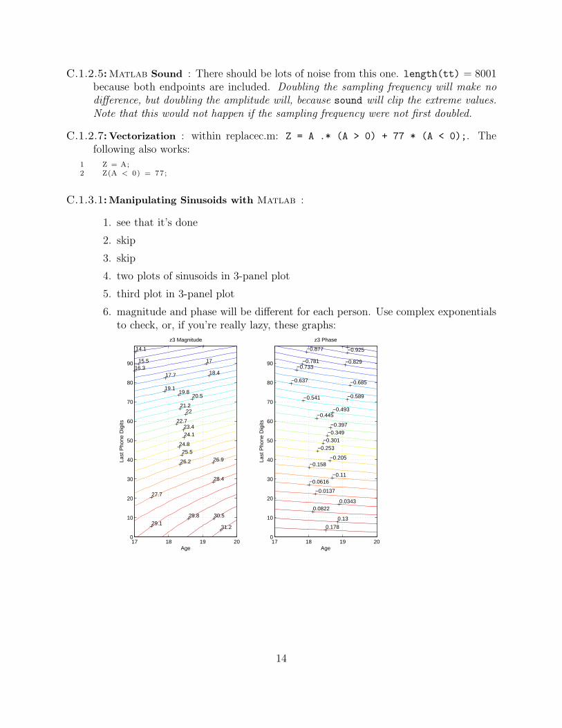
C.1.3.1:Manipulating Sinusoids with Matlab :

1. see that it’s done

2. skip

3. skip

4. two plots of sinusoids in 3-panel plot

5. third plot in 3-panel plot

6. magnitude and phase will be different for each person. Use complex exponentialsto check, or, if you’re really lazy, these graphs:

17 18 19 200

10

20

30

40

50

60

70

80

90

14.114.8

15.516.3

17

17.7 18.4

19.119.8

20.5

21.222

22.723.424.1

24.825.5

26.2 26.9

27.7

28.4

29.129.8 30.5

31.2

Age

Last

Pho

ne D

igits

z3 Magnitude

17 18 19 200

10

20

30

40

50

60

70

80

90

−0.973−0.925−0.877

−0.829−0.781−0.733

−0.685−0.637

−0.589−0.541

−0.493−0.445

−0.397−0.349

−0.301−0.253

−0.205−0.158

−0.11−0.0616

−0.0137

0.03430.0822

0.13

0.178

Age

Last

Pho

ne D

igits

z3 Phase

14

4 Lab 2: Introduction to Complex Exponentials

Ingredients: C.2.2.1: Complex Numbers, C.2.2.2: Sinusoid Synthesis with an M-

File, C.2.3.2: Verify Addition of Sinusoids Using Complex Exponentials,C.2.4: Periodic Waveforms

Indications: relation between sinusoids and complex exponentialsWarnings: noneDirections: see belowLast Used: Fall 2003, Spring 2004

Some labs are built around verifying theory, others around exploring an application. Inaddition, many try to expand one’s abilities in Matlab. A useful improvement to thiscourse would be to specify some of each approach in each lab, as is done in this lab.

4.1 Introduction

Show the use of zvect, zprint, and zcat, by essentially doing section C.2.2.1: Complex

Numbers for students, on the projector screen.

This is a relatively self-explanatory lab, but here are a couple of notes.

4.1.1 Fixing zvect and zcat

Replace the line if( vv(1)==’5’ ) in zvect and zcat with if( vv(1)==’5’ || vv(1)==’6’

) and then reload Matlab. Otherwise, these functions will not work.

4.1.2 Explaining sumcos

I think C.2.2.2: Sinusoid Synthesis with an M-File is one of the most clever problems in thebook, and well worth a little frustration on the students’ part. In this problem, one wantsto generate a sum of sinusoids given their fundamental information (frequency and phasor).The challenge is to manipulate the values so as to do most of the calculation in a way thattakes advantage of Matlab’s optimized matrix multiplication.

It is one of the mind-blowing results of Signals and Systems that any periodic function can beproduced by adding together sinusoids of the right amplitudes, frequencies, and phase shifts. The

15

first exercise, writing sumcos is just a way to do that efficiently in Matlab and it will be usefulto us later.

There are three areas where you have to make intellectual leaps: How complex numbers canbe used for magnitude and phase; how some matrix elements map to pieces of your sinusoidequation; and how to make the matrix math combine the right pieces.

At this point, you can let them work for a while (read the problem and try to figure itout), or you can give in and help them some more. You may also want to explain matrixmultiplication (which indices are summed over) and how to take a transpose in Matlab

(the ’ operator).

Here is the mapping you want:

complex exponent summing matrix math︷︸︸︷

x′(t) =L∑

k=1

ej2πfktXk ↔︷︸︸︷

cn =L∑

k=1

ankbk

Seen another way, you want to make Matlab calculate:

(

x′(0) x′( 1fs

) x′( 2fs

) · · · x′(tdur))

=

(

X1 X2 · · · XL

)

e0 e2πf11

fs e2πf12

fs · · · e2πf1tdur

e0 e2πf21

fs e2πf22

fs · · · e2πf2tdur

......

.... . .

...

e0 e2πfL1

fs e2πfL2

fs · · · e2πfLtdur

Note that the number of elements for each dimension works out: there are L sinusoids to sum,and N (for the index n) elements of time.

For matrix subscripts, the first element denotes the rows, the second the columns. So you firstneed to make the elements of the a matrix above be such that each element corresponds to adifferent pairing of time and sinusoid. You will need to use transpose to do this.

When you’re all done, you need to convert the complex exponentials to cosines by taking the realpart of your results (this is why I use x′ above).

The way to tackle this problem is to start by combining t and f ; then make that into the exponentof a complex exponential; then multiply by X; then take the real part.

16


4.2.1 Student Supplement

Test your sumcos (see C.2.2.2: Sinusoid Synthesis with an M-File)! In Matlab, xx = sumcos(25*(1:25),

(1 + j) ./ (1:25), 1000, .1) should result in the following graph (after proper labeling):

0 0.02 0.04 0.06 0.08 0.1−2

−1

0

1

2

3

4Sumcos Litmus Test

t = 0:(1/1000):.1

x =

sum

cos(

...)

C.2.3.2: Verify Addition of Sinusoids Using Complex Exponentials is not very clear on its overallgoal. They want to show that if you do math with complex exponentials, you will get the sameresults as if you had added together full sinusoids. The process that it wants you to follow is this:

1. Generate four sinusoids.

2. Add them together to get a fifth sinusoid.

3. Measure the magnitude and phase of the summed result.

4. Generate five complex exponentials, including your measured results, using commands likez = A * exp(j*phi), where A and phi are the values that you were given or measured.

17

5. Add together the first four complex exponentials. The result should be approximately equalto the fifth complex exponential.

In the last step, you can confirm the result by showing the numbers, but you should also confirm itgraphically. Use zcat to graphically add (by concatenating end-to-end) the first four exponentials.Using hold and zvect, plot the last exponential on the same graph. The results of zvect andzcat should point to the same place, making a closed loop.

4.3 Deliverables

• Matlabiness: C.2.2.2: Sinusoid Synthesis with an M-File: Complete the definition ofsumcos; include the three plots from the end of the section

• Verification: C.2.3.2: Verify Addition of Sinusoids Using Complex Exponentials: Do all 7parts, except for the verification in part 2.

• Application: C.2.4: Periodic Waveforms: Do parts 1 and 3.

4.3.1 Grading

C.2.2.2:Sinusoid Synthesis with an M-File : Within sumcos: a check that f and X havethe same length, and xx = real(X*exp(j*2*pi*f.’*[0:1/fs:dur]));.

C.2.3.2:Verify Addition of Sinusoids Using Complex Exponentials :

1. see part 3

2. skip verification, and see part 3

3. 5 plots: x1, x2, x3, x4, and x5 = x1 + x2 + x3 + x4, with a few periods of each.

18

4. A = 4.69, φ = 1.5.

5. zprint will give the results in both forms.

z1 = 5∗exp ( j ∗ . 5∗ pi ) = j5z2 = 5∗exp(− j ∗ . 25∗ pi ) = 3.535 − j 3 . 535z3 = 5∗exp ( j ∗ . 4∗ pi ) = 1 .545 + j4 . 755z4 = 5∗exp(− j ∗ . 9∗ pi ) = −4.755 − j 1 . 545z5 = 4.686∗exp(− j ∗ . 1 . 5 01∗ pi ) = 0 .3253 + j4 . 675

6. A plot of vectors where one from the origin ends at the same point as anotherstream of four vectors.

7. Magnitude and phase correspond to amplitude and phase shift.

C.2.4:Periodic Waveforms :

1. A beautiful square wave

2. Sound grows harsher

3. A beautiful sawtooth wave

19

5 Lab 3: Synthesis of Sinusoidal Signals

Ingredients: C.3.2.3: Piano Keyboard, C.3.3: Synthesis of Musical Notes

Indications: sinusoids ↔ sounds, harmonicsWarnings: noneDirections: allow 2 weeks for full effectLast Used: Fall 2003, Spring 2004

This has consistently been one of the student’s favorite labs.

5.1 Introduction

I start by showing off past songs, to get people excited about making their own.

The goal of this lab is to make a song, with both a treble and a bass line, that sounds plausible.You have more freedom in this lab than the previous ones. I’m going to describe one way toapproach this problem, but there may be others, which you’re welcome to pursue.

We can input our songs as arrays of numbers, which index the keys on a piano, and durations.There are 88 keys on a piano, so the piano-key-numbers will range from 1 to 88.

20

5.1.1 Minimal Music Theory

The simplest way to make a song is by stringing together a series of sinusoids of the appropriatefrequencies (the frequency produced by pressing a given piano key). There exists a straight-forward relation between the frequencies used in music, and we will use that to translate thepiano-key-numbers into frequencies.

Music frequencies are on a logarithmic scale– your ear hears tones as related when one is a simplefraction multiple of the other. The most closely related tones are said to be “one octave apart”,and this corresponds to the higher frequency being exactly twice the lower frequency. On a piano,there are 12 notes within each octave; twelve frequencies are used between a given note and thenote with twice its frequency.

During the Baroque era, keyboardists adopted “equal-tempering”– that is, having every noterelated to the one after it by the same multiplicative factor. Since there are twelve notes in eachoctave, and after those twelve notes you need to have a doubling of frequency, that multiplicativefactor is none other than 21/12.

Now all you need is one reference and you have every note. Traditionally, that reference is the Aabove middle-C, key 49, with a frequency of 440 Hz.

Now it’s just a matter of data input to get old video-game quality music.

5.1.2 Harmonics and Other Improvements

Pure sinusoids won’t sound very realistic, but there are several things that you can do to improveyour song. One is to use “harmonics”, adding several higher frequencies, all of which are multiplesof your original frequency. As you saw with sumcos, the result will still have the original frequency,but a different shape. Every instrument has a characteristic pattern of harmonics, and these arewhat largely give its sound its quality.

This is also what distinguishes different vowel sounds in speech. A vowel sound is characterizedby a particular pattern of harmonics of whatever pitch of the person’s voice is at (the fundamentalfrequency). The sound ’aaaaahhh’ sounds different from a pure sinusoid because it has othersinusoids added in. However, the frequencies of all those other sinusoids are multiples of the pitchfrequency, so that final signal still has the same period as the pure sine wave. ’Aaahhh’ soundsdifferent from ’eeeehhh’ because of how large each of those harmonics is.

Another way to improve the sound is to multiply each note by an “envelope”. The notes will soundmore realistic if their volume changes over their duration the way it would if played on a piano:

21

getting loud at one moment and slowly dying off later. Since volume corresponds to the magnitudeof the sinusoids, we can cause this effect by multiplying the sinusoids by an appropriately shapedfunction. This is ADSR scaling (attack, delay, sustain, release) and C.3.3.3: Musical Tweaks

explains it more.

The best way to approach this lab is to do C.3.2.3.2, writing the tone function, and thenC.3.2.3.3, the play scale function. You can modify these to make your song and add additionalfeatures. If you need more background, you probably want to read through from the beginningof the lab.


5.2.1 Student Supplement

The two improvements that will probably make the largest effect are ADSR scaling and harmonics(see C.3.3.3: Musical Tweaks).

If you do the warm-ups, ignore the malicious amplitude A = 100 in C.3.2.2.1. Use A = 1.

The following data files, with notes and durations, are available for your use, in the matlab

directory.

22

Song Title Artist/Composer Data Input FilenameJesu, Joy of Man’s Desiring Bach Ben Donaldson jesu.m

Fur Elise Beethoven DSPFirst Authors furelise.m

Minuet in G Bach Nick Zola minuteg.m

The Girl from Ipanema Antonio Carlos Jobim Ransom Byers thegirl.m

Gigue Fugue BMV 577 Bach Katerina Blazek fugue577.m

Cannon in D Pachelbel Jeffrey Satwicz LOST!Final Fantasy Song Unknown Chris Murphy finalfant.m

Twinkle, Twinkle Little Star Mozart James Krejcarek twinkle.m

Fifth Symphony Beethoven Kevin Tostado bfifth.m

Carol of the Bells Peter J. Wilhousky Daniel Lindquist carolbells.m

Variation Jacob Graham Jacob Graham variation.m

The Parting Glass2 Traditional Caitlin Foley partglass.m

Popular Stephen Schwartz Jerzy Wieczorek popular.m

Tears in Heaven Eric Clapton Jay Gantz tersheaven.m

Toki ni Ai Wa from “Shoujo Kakumei Utena” Mikell Taylor tokiniaiwa.m

Suite Bergamasque 4th Movement, Passepied Claude Debussy Frances Haugen passepied.m

My Immortal Evanescence Amanda Blackwood immortal.m

5.2.2 Question Help

The ADSR envelope can be difficult, depending on how it is approached (see C.3.3.3: Musical

Tweaks). One systematic way to do it is by choosing slopes and intercepts, than thenprogramming equations for each of the form y = mx + b. However, note that this equationmust take into account the length of the note, which will change the slope.

The easiest way is to use linspace and vector concatenation.

5.3 Deliverables

Create one song (treble and bass), plus two “improvements”. You may use song data alreadywritten or write your own. Writing your own song counts as one improvement, so if you doyou only need one more.

2A fine Irish drinking song:

Of all the money ere I had, I spent it in good company,And all the harm I’ve ever done, alas was done to none but meand all I’ve done for want of wit, to memory now I can’t recallso fill me to the parting glass, good night and joy be with you all.

23

An improvement might be:

• ADSR envelope scaling, described in the book

• Removal of any clicks in the sound (by a method other than ADSR)

• Addition of harmonics

• Inputting your own song (rather than one from the CD or the archive)

• A clever structural improvement on your song synthesis program design (e.g. usingsumcos for making chords)

• Something else

An improvement in general should be something “m-file-able”, which can be applied to anysong. Tweaking numbers yourself to make the song sound better does not count.

Please turn in:

• The original song (m-file and wav-file (use wavwrite))

• The original plus one improvement (m-file and wav-file)

• The original plus the other improvement (m-file and wav-file)

• The final version, with all improvements applied

5.3.1 Grading

You can use Window Media Player’s “Scope” visualization to see the waveforms in the wav

files. Here you can immediately see harmonics, clipping, and diagnose some problems. Below,for example, is song with an envelope (good!) and clipping (bad!).

24

Write to the authors of any songs that particularly impress you or nicely complement thosein the archive. Ask if you can add their song for future generations to use.

6 Lab 4: AM and FM Sinusoidal Signals

Ingredients: C.4.4: FM Synthesis of Instrument Sounds, C.4.5: Woodwinds

Indications: harmonics, chirps, instantaneous frequencyWarnings: noneDirections: see belowLast Used: Fall 2003, Spring 2004

6.1 Introduction

I don’t remember well how I combined the three interrelated topics here: instantaneousfrequency (of which chirps are the simple example), speech signals (an example of an “in-teresting” variable frequency signal), and reading spectrograms. Many combinations work,and I’ve used more than one.

6.1.1 Instantaneous Frequency

Up to this point, we’ve have only considered linear combinations of sinusoids with constantfrequencies– with frequencies that weren’t changing in time. However, most interesting, realworld signals are not so simple.

Chirps are useful as a simple example of changing frequency. Chirp frequency changes linearly.In this lab, we’re going to make signals that ultimately change very quickly and sinusoidally.

Mathematically, the instantaneous frequency of a signal is based on the derivative to the argumentto cosine function. So the chirp function y(t) = cos(πt2) has a angular frequency functionωi(t) = 2πt and a frequency function fi(t) = t.

6.1.2 Reading Spectrograms

In class, we’ve looked at the spectrum, or frequency domain representation, of a signal. Thespectrum of a signal represents that signal for all time, but often it is useful to consider the

25

frequencies present “around” each moment in time and see how those frequencies change intime. This is the one of the best representations for what our ears hear.

The songs that you made in lab 3 might look like this: (show a series of dashes at variousheights in a spectrogram).

A chirp signal would look like this: (show a sloped line).

Speech will look much more complicated, but if you have a clear enough signal, you will still beable to identify changing frequency bands: (show a “thumb print-like pattern” of rising andfalling harmonics). As an example of this, many English vowels are diphthongs, which meansthat they “slide” from one to another. The word “slide” has a diphthong /ai/. On a spectrogram,we would see a shift from one harmonic signature to another. Borrow from 5.1.2 here as needed.

DSPFirst provides a great function to display spectrograms, called specgram. It has threeparameters: specgram(signal, ws, sampfreq). Explain the three parameters (see B.2).Show examples on the screen. For the default, you can use [] for the second parameter.

By increasing the second parameter to specgram, I can improve the vertical resolution, but atthe same time I lose horizontal resolution. If I decrease it, the opposite happens. (Show this onthe projector.) I cannot get perfect resolution both horizontally and vertically, both because ofthe sampling rate, and for reasons related to the Heisenberg Uncertainty principle.

At the end of the introduction, help students who don’t have specgram. Some may haveit, depending on what classes they have already taken. Those who don’t have to install theSignalProcessingToolbox for Matlab, in \\Stuapp\NETAPPS\ under Matlab. The PLPkey that the install program asks for is in \\Stuapp\Licences\ under Matlab. Afterinstalling the toolbox, make sure that the DSPFirst directory is still listed in Matlab’spath.

For reasons that I don’t fully understand, when the frequency of a signal changes sinusoidal,and does so quickly enough, it sounds like it has a particular set of harmonics. Moreover, forless obscure, but more hand-wavy reasons, these harmonics happen to sound very much like realinstruments (the effect sounds like the effects of the vibrating material of the instrument).



• When using the FM synthesis equation, let φm = φc = −π2

(see C.4.4: FM Synthesis of

Instrument Sounds).

26

• Bell Lab Clarifications (see C.4.4.2: Parameters for the Bell)

– Use A0 = 1 for the amplitude envelope.

• Clarinet Lab Clarifications (see C.4.5: Woodwinds)

– In place of Aenv and Ienv as arguments to clarinet(), use A0 and I0, whichshould just multiply the envelopes that you produce using the instructions in thelab in C.4.5.1: Generating the Envelopes for Woodwinds.

– In the example for plotting woodwenv(), replace delta with 0.

– Error: Index exceeding matrix dimensions when using woodwenv

The vectors produced by woodenv have one fewer elements than would usually beexpected. You have to scale other vectors that you use with the vector producedby woodenv (for example, when multiplying two vectors) down to the its length.For example, to plot y1 from woodenv vs. tt, use plot(tt(1:length(y1)), y1).

6.3 Deliverables

• Do one of the sound synthesis lab parts in Lab B (either C.4.4, the bell, or C.4.5, theclarinet).

• Do all 6 parts on page 451 (the last part of the bell lab) for the instrument of yourchoice, for one set of parameters (one note – pick your favorite). Use wavwrite tosave the your favorite sound.

6.3.1 Grading

These answers will vary depending on which set of parameters and instrument is chosen bythe student.

C.4.4.3:The Bell Sound :

1. It should sound something like the instrument.

2. For the bell, look at the bottom two stripes in the spectrogram and take thegreatest common divisor. This is a given for the clarinet functions, which specifytheir fundamental frequency, but students should still verify it.

3. The sound will go from many harmonics to few. fi(t) will look a lot like f(t), butvertically offset to the fundamental frequency.

27

This has an offset of 110 Hz.

4. Harmonic structure is the presence of various “bars” in the spectrogram.

5. The amplitude of the signal will follow the envelope provided.

6. The zoomed-in signal will look very different depending on where it is taken.

28

7 Lab S: Sampling and Aliasing

Ingredients: Appendix FIndications: effects of samplingWarnings: noneDirections: see belowLast Used: Spring 2004

The lab is provided in the appendix. This and Lab C were intended to fill the gaping holein DSPFirst’s schedule of labs.

7.1 Introduction

The last part of this lab is a signal processing pitch adjustment system, which allows oneto shift all of the tones in a piece up or down in frequency. I think that my system is agood example of signal processing, and useful for encouraging systems-thinking and learningto mentally manipulate spectrum graphs (similar to the advantages of teaching AM radiomechanics). So my introduction starts with asking how one might go about doing this kindof pitch adjustment.

One method, more procedural than mine, is to take segments of the audio clip, man-handlethem by shifting their frequency peaks to any particular place, and then recompose thesegments (this works well when you overlap the segments). Another method is to interpolatedata points every so-often. My method is cute, but ultimately flawed because it doesn’tincrease tones exponentially.

The rest of the introduction is for describing my system (see F.2), and why we needed anextra lab here.

7.1.1 Tone Shifting System

In class, I would expand more on the sketched explanation below. Use graphs like those inAppendix F.2 to complete the description.

The basic idea behind my tone-shifting system is to use basic multiplication of the signal by asinusoid to adjust the frequency, and filtering to remove any unwanted extra frequencies thatresult. The normal problems with this come from aliasing and what happens when previouslynegative frequencies peaks overlap positive peaks. Show the futility of trying to fix this problem

29

using just multiplication by sinusoids and filtering. To solve this problem, another constraintis needed: that the signal is sufficiently band-limited that it can be downsampled by 2 withoutlosing important information. In other words, the original sampling must be at twice the Nyquistfrequency. Then we can (1) shift the frequency-domain forms into the extra frequency space, (2)keep only the “inside” halves of each form, (3) subsample by 2, which corresponds to shifting theNyquist frequency in, and (4) shift the result by the Nyquist frequency to recenter the forms.


7.2.1 Question Help

In Appendix F.1.1, remember that the instantaneous frequency is not just whatever ω(t) is incos(ω(t)t+φ). It’s actually the derivative of the argument to cos(.). That means that for chirps,there’s an extra factor of 2 that you might not expect.

Some students will forget to provide the arguments to specgram to properly scale the axes oftheir spectrograph. This is particularly common for the first chirp problem, where a properscaling reveals that the student has forgotten the doubling effect of the quadratic term.

7.3 Deliverables

• Do either sections S.1.1 - S.1.3 of the lab, or do sections S.1.1 and S.2.

7.3.1 Grading

F.1.1 :

1. A spectrogram with a sloped line near the bottom, from 200 Hz to 800 Hz.

30

2. A spectrogram that quickly reaches the top, goes down, and back up.

F.1.2 :

1. nothing expected

2. Make sure that the graphs meet the requirement that some lower-sampled graphhas a higher apparent frequency than some other higher-sampled graph. This willbe the most difficult for students who are randomly choosing values.

31

F.1.3 :

1. nothing expected

2. spectrogram of song with clear bars

3. spectrogram, with some bars “looped-over the top”.

32

This graph used an incorrect sampling fre-quency.

F.2 :

1. Plot of a sinc function.

2. nothing expected

3. .wav file with adjusted frequencies. Some sloppiness will be apparent if the lowpass filter is only applied once.

4. m-file of commands

Below is an example of what actually happens. Each graph corresponds to a theoreticalgraph from F.2.

33

−1 −0.5 0 0.5 1

x 104

100

200

300

400

500

600

700Original Signal

ω

X(ω

)

−1 −0.5 0 0.5 1

x 104

100

200

300

400

500

600

700Low−passed Signal

ω

U(ω

)

−1 −0.5 0 0.5 1

x 104

50

100

150

200

250

300

350

400

Shifted Signal

ω

V(ω

)

−1 −0.5 0 0.5 1

x 104

50

100

150

200

250

300

350

400

Middle−clipped Signal

ω

W(ω

)

−1 −0.5 0 0.5 1

x 104

20

40

60

80

100

120

140

160

180

200

Subsampled Signal

ω

Y(ω

)

−1 −0.5 0 0.5 1

x 104

50

100

150

200

250

300

350

400

Recentered Signal

ω

Z(ω

)

1 function zz = p i t chad j (xx , f s , f x )2 % Adjust the p i t c h o f a sound sample ( xx ) by a smal l amount ( f x ) . The3 % r e s u l t w i l l have ha l f t he o r i g i n a l sampling f requency ( f s /2) .45 f i l t s i z e = 200 ;6 warning o f f MATLAB: divideByZero ;78 W = 2∗pi ∗( .25 − f x / f s ) ;9 n = − f i l t s i z e /2 : f i l t s i z e /2 ;

10 lowpass = sin (W∗n ) . / ( pi∗n ) ;11 lowpass ( f i l t s i z e /2 + 1) = W / pi ;1213 f igure ( 1 ) ;14 showdblspec ( xx , f s , ’ O r i g i na l S i gna l ’ , ’X ’ )1516 uu = conv( xx , lowpass ) ;17 uu2 = conv(uu , lowpass ) ;1819 f igure ( 2 ) ;20 showdblspec ( uu2 , f s , ’Low−passed S igna l ’ , ’U ’ )2122 tt1 = 0:1/ f s : ( ( length ( uu2 ) − 1 ) / f s ) ;23 mod1 = cos ( (2∗ pi ∗( f s /4 − f x ) ) ∗ t t1 ) ;24 vv = uu2 . ∗ mod1 ;2526 f igure ( 3 ) ;27 showdblspec ( vv , f s , ’ Sh i f t ed S igna l ’ , ’V ’ )2829 ww = conv( vv , lowpass ) ;

34

30 ww2 = conv(ww, lowpass ) ;3132 f igure ( 4 ) ;33 showdblspec (ww2 , f s , ’ Middle−c l i pped S igna l ’ , ’W’ )3435 yy = ww2 ( 1 : 2 : end ) ;3637 f igure ( 5 ) ;38 showdblspec ( yy , f s , ’ Subsampled S igna l ’ , ’Y ’ )3940 tt2 = 0:2/ f s : ( ( length ( yy ) − 1 ) / ( f s / 2 ) ) ;41 mod2 = 2∗cos ( (2∗ pi∗ f s / 4 ) ∗ t t2 ) ;42 zz = yy . ∗ mod2 ;4344 f igure ( 6 ) ;45 showdblspec ( zz , f s , ’ Recentered S igna l ’ , ’Z ’ )4647 function showdblspec ( xx , f s , name , var )48 plot ( linspace (− f s , f s , length ( xx ) ) , abs ( f f t sh i f t ( f f t ( xx ) ) ) ) ;49 t i t l e (name ) ;50 xlabel ( ’ {\omega} ’ ) ;51 ylabel ( [ var ’ ({\ omega}) ’ ] ) ;52 axis t i gh t ;

8 Lab C: Convolution Lab

Ingredients: Appendix G.3Indications: convolutionWarnings: the first parts haven’t been tried; use Simulink instead?Directions: see belowLast Used: Fall 2003

The lab is provided in the appendix. After presenting what was needed, I told students tostart on the third part. After seeing the confusion and time that that section elicited, Idecided to cut out the other parts.

8.1 Introduction

Often students will not have a good sense of how convolution works, although it will havebeen presented in class. I gauge the class knowledge and teach the impulse and graphicalmethods as needed. Then I explain the application of convolution to the lab.

It turns out that samples of a sinusoid of a particular frequency, used as the elements of a filter,create a narrow band-pass filter, right around the frequency of the sinusoid. There are two waysto understand this:

35

1. Think about applying this filter to a pure sinusoidal signal, in the time domain. Theconvolution sum turns into a sum of the product of the two sinusoids at every point. Now,summing the product of two sinusoids of the same frequency is constructive interference,and the result will be large; if the sinusoids are different frequencies, that’s destructiveinterference, and the result will be small.

This comes from the fact that,

∫∞−∞ cos(ω1t) cos(ω2t) =

{

0, ω1 6= ω2

∞, ω1 = ω2,

which, for those who know linear algebra, means that sinusoids of different frequencies areorthogonal, and therefore appropriate basis functions.

2. The spectrum of a sinusoid is just two spikes. That means, directly, that the frequencyresponse of samples of a sinusoid, used as a filter, will also just have two spikes. Convolutionin the time domain is multiplication in the frequency domain, so convolving a signal witha sinusoid is equivalent to multiplying the spectrum of that signal by the spectrum of thesinusoid, which is 0 everywhere except for the peaks. So we have filtered out (or zeroedout) everything but the frequencies spikes that line up with those of our sinusoid. In otherwords, a signal is a filter.

Finally, if you add together a lot of sinusoids of particular frequencies, you can get a filter withpeaks in all of those locations. If you choose your frequencies to correspond to those of an piano,anything that you filter will sound a bit like it was played on an organ.


To plot a spectrum in Matlab, use plot(abs(fft(data))). Note that fft has low posi-tive frequencies to the left, increasing frequencies to the right to the Nyquist frequency inthe center, then minus the Nyquist increasing to 0 again. In other words, the horizontaldimension is evenly divided between 0 and 1, rather than -.5 to .5, as we usually use.

Many .wav files available online are incompatible with Matlab. It often takes some lookingaround to find one that will work.

Often the note-pass filter will result in eerie sounds, with the song quiet in the background.This happens either because the song is off key, relative to the filter, or because the filteris “smearing” out the each impulse in the song over too long a time. To account for thefirst problem, graph the spectrum of the signal and look for the peaks. To account for thesecond, you use a smaller filter, but this will make the filter less precise, so these problemsare not entirely fixable.

36

8.3 Deliverables

• Just do lab section C.3 (Demo Soundtrack). As listed in the document. Turn in allanswers to questions.

8.3.1 Grading

E.3.1 : A spectrogram of the song (regions of energy should be clearly visible).

E.3.1 : First, a note-pass filter created with sumcos. Second, a .wav result of the filterapplied to the song.

9 Lab 5: FIR Filtering of Sinusoidal Waveforms

Ingredients: C.5.3.1: Filtering Cosine Waves - C.5.3.4: Time Invariance of the Filter

Indications: LTI-ness, FIR filters, filtering sinusoidsWarnings: a bit dryDirections: see belowLast Used: Fall 2003, Spring 2004

This is basically a “verify the theory” lab.

9.1 Introduction

The filter that we will use in this lab is the first difference filter– an incredibly useful filter. It isthe archetypical high-pass filter, closely related to differentiation, simple negative feedback, andedge-detection.

The lab is generally straightforward, but here are a couple of places to watch out for:

• There is a difference between the result of firfilt and the filtering that it represents.Namely, firfilt gives back all the data, but gives no information as to its whereaboutson the x-axis. You can, however, display the data wherever you wish, using the functionsplot and stem.

• stem takes the same arguments as plot, but makes cute stem-plots of the data. It’spossible to call stem with just one argument, stem(data), where the x values correspond

37

to the indices of the data vector. This makes plots that go from 1 to some N . However,in the first part of this lab, you filter values from a cosine wave which has its first value atn = 0, which means that, for this filter, the output should appear on the graph to start at0. Thus the cryptic comment, “Use the stem function to make a discrete-time signal plot,but label the x-axis to span the range 0 ≤ n ≤ 49.” (see C.5.3.2: First Difference Filter)

• It may be more difficult to determine the magnitude and phase of some of the graphs,because there aren’t as many points. Just make an educated guess, by drawing the sinusoidthat would naturally go through the points that you have. Note that the magnitude of thissinusoid will generally be larger than the maximum point height– that’s okay.

• Part 6 asks you to characterize the filter’s performance (see C.5.3.2: First Difference Filter).In other words, you put a sinusoid into the filter, and got a sinusoid out– with the samefrequency but a different amplitude and phase shift. For an LTI-system, knowing what afilter does to one example of a sinusoid of a particular frequency is all we need to knowwhat it does to all sinusoids of that frequency (dazzle with math here as needed, to showthat it’s the ratio of amplitudes and difference of phases that are needed to characterizethe filter.) So you can check the filter out from one example in part 6, and work backwardsfrom the general form in part 7, and get the same result.

• The rest of the lab shows linearity and time-invariance. You don’t have to do all parts 1-7for each example; just whatever is needed to similarly characterize the filter’s “behavior”in each instance.

9.2 Deliverables

All answers and graphs in C.5.3.1: Filtering Cosine Waves - C.5.3.4: Time Invariance of the

Filter, except C.5.3.2.3. That is C.5.3.2: First Difference Filter: 1, 2, 4-7; C.5.3.3: Linearity

of the Filter: 1-3; C.5.3.4: Time Invariance of the Filter.

9.2.1 Grading

C.5.3.2 :

1. l(y[n]) = l(x[n]) + l(bb) − 1 = 50 + 2 − 1 = 51

2. Plot: 2 sinusoids, 0-crossings: +- @ 2.5; -+ @ 6.5

38

3. skip

4. first sample different because x[−1] = 0 (other similar reasons work too)

5. a = 14, φ = 616

2π = .75π = 2.3562

6. A = 2, φ = .417π = 1.31

7. A = 1.95, φ = 1.37

C.5.3.3 :

1. Plot: Same a and φ from C.5.3.2.5

2. Plot: a = 3.9, φ = .375π = 1.18

3. Plot: graphs are equal

39

C.5.3.4 :

1. Plot: 3 samples to align

10 Lab 6: Filtering of Sampled Waveforms: Cascading

Systems

Ingredients: C.6.3.1: Filtering a Stair-Step Signal - C.6.3.6: Comparison of Systems

Indications: frequency response, low/high pass, (cascading filters)Warnings: dry and abstractDirections: see belowLast Used: Fall 2003

40

10.1 Introduction

The last lab was a “verify the theory lab”. This is an “explore the theory” one.


Use plot, rather than stem, to generate your graphs. When plotting the input and output of asignal on subplots of the same window, make sure they both line up at n = 0 and clip both tothe length of the input signal. x1 comes from the command load lab6dat.

10.2.1 Question Help

How do I find the impulse response of the cascaded system in C.6.3.4: Implementation of First

Conceptually, you can put in an impulse and see what happens to it. That is, if you put animpulse into the first system, you’ll get its impulse response out, which will be the input tothe second system, and the result will be the impulse response of the combined systems.

10.3 Deliverables

• As in the lab, C.6.3.1: Filtering a Stair-Step Signal - C.6.3.6: Comparison of Systems:mostly plots and some writing.

10.3.1 Grading

C.6.3.2: Implementation of 5-Point Average :

1. v1 = firfilt(ones(1, 5) / 5, x1);

Plot input, output in 2-panel subplotQualitative description: smootherTime shift: 2 samples

41

2. freqz magnitude plotFrequencies passed: 0, 1.901 = 3

5π, π

Frequencies rejected: ±1.256 = 25π,±2.515 = 4

5π

Qualitative relation: doesn’t let through jagged stuff

3. freqz angle plot Measure slope: (2 ∗ −2.5/2.515) ≈ −2

C.6.3.3: Implementation of First Difference System 1. v2 = firfilt([1, -1], x1);

Plot input, output in 2-panel subplot

42

2. Qualitative description: pointy; derivative

3. freqz plotsQualitative relation: only lets changes throughHigh pass filter

(slope: (3.12/2π) = 1/2; shift = .5 samples)

C.6.3.4: Implementation of First Cascade 1. y1 = firfilt([1, -1], v1);

Plot

2. freqz(conv([1, 1, 1, 1, 1], [1, -1]), 1, omega);

Plots

43

C.6.3.5: Implementation of Second Cascade 1. y2 = firfilt(ones(1, 5) / 5, v2);

Plot

2. freqz(conv([1, -1], [1, 1, 1, 1, 1]), 1, omega);

Plots

Graph is visually identical to the above.

C.6.3.6:Comparison of Systems 1. Calculate error: about 1.6384 × 10−29

In the future, to find time shift for C.6.3.2: Implementation of 5-Point Average, ask for a plotshifted with the claimed time shift over the original.

11 Lab 6: Filtering of Sampled Waveforms: Filtering

the Speech Waveform

Ingredients: C.6.3.7: Filtering the Speech Waveform and supplemental problemsIndications: filtering in frequency domainWarnings: noneDirections: see belowLast Used: Spring 2004

11.1 Introduction

Fix inout. See 11.2.1 below.

44

Make sure that the concept of filtering in the frequency domain is understood, and discussit as needed, including how to do it, how it is related to convolution, and how to understandit graphically.


x2 can be loaded with the command load lab6dat.


inout won’t graph anything! Change line 69 of striplot.m (in the toolbox/dspfirst

directory) to read “if (vv(1)==’5’ || vv(1)==’6’)”. Then reload Matlab.

11.3 Deliverables

• Questions 1-8 (all parts) of C.6.3.7: Filtering the Speech Waveform:Plots may be saved and included in your lab report or lab folder, or generated by anm-file included in your lab folder. Each part asks for a “doing” (plots in 1-6, listeningin 7 and 8) and a “commenting”.

• Generate the spectrogram of the first 20000 points of x2, y1, and y2.

• Generate the spectrum of x2, y1, and y2 using abs(fft(x2)). The samples of theseresults correspond to values of ω from 0 to 2π. Scale your x-axis on your plots accord-ingly (but ignore the scaling on the y-axis).

• Convolve h1 and h2 to get a new filter h3. Look at its frequency response using freqz.How do you think it will affect the signal? Use firfilt to apply it and comment on theresults (you may wish to refer to a spectrum, spectrogram, or sound in your comments).

11.3.1 Grading

C.6.3.7:Filtering the Speech Waveform :

1. I would call it smoother

45

2. Note big hump near 0

3. The coefficients form a sinc function

4. I would call it rougher

46

5. Note the big ditch near 0

6. Almost a sinc function, except the center point

7. all frequencies; low frequencies; high frequencies

8. The sum will again have all frequencies, because the sum of the filters is animpulse, and the sum of H1 and H2 is all-pass.

Spectrograms See the unfiltered frequencies as having dark red energy.

47

Spectra See the spectrum attenuated in the appropriate areas

Combined Create a sort-of bandpass or no-pass filter where the low and high-pass filtershave their slopes.

48

12 Lab 7: Everyday Sinusoidal Signals: Telephone Touch

Tone Dialing

Ingredients: C.7.1.1: Telephone Touch Tone Dialing, C.7.1.2: DTMF Decoding,C.7.2.1: DTMF Dial Function, C.7.4: DTMF Decoding

Indications: filteringWarnings: too much coding, too little S&S?Directions: see belowLast Used: Fall 2003

12.1 Introduction

Telephone tones are composed of two sinusoids of different frequencies added together. Thatmeans, for engineers like us, it’s easy to compose signals that fool the phone companies, anddecode signals just like the phone companies. That’s what this lab is all about.

Composing signals is easy– you’ve already done it in lab 3. Decomposing them requires only asmall conceptual hurdle: filtering as a way to “detect energy”.

12.1.1 Detecting Energy

Detecting energy in signals sounds mystical, but if we leave the deep aspects to the “Philosophyof Signals and Systems” class, all it means is determining the frequencies apparent in a signal.Potentially, any signal is composed of sinusoids of all frequencies, but it will have most of themat an imperceptible level– their magnitude will be approximately 0. On a graph of the spectrumof a signal, those areas that are non-zero are said to have energy. For example, a signal mighthave energy in the low frequencies, or the high frequencies, or around 440 Hz.

If you apply a low-pass filter to a signal with energy in low frequencies, the result will be non-zero;if you apply a high-pass filter to the same signal, the result will be near zero. So filters can beused to find where a signal has energy– they can “detect” energy.

The lab is very readable, so I’ll leave you to follow the rest. Watch out for the amplitudemodulation sections that are interwoven through the lab and don’t read them unless you wantto– they apply to a different assignment. Specifically, you want to look at C.7.1.1: Telephone

Touch Tone Dialing, C.7.1.2: DTMF Decoding, C.7.2.1: DTMF Dial Function, and C.7.4: DTMF

Decoding.

49

After making the lab’s functions, you might have fun trying these out on a few of your friends orenemies.

Also, when you are trying to compose your phone signal, you can use dtmfchck to check yourwork (for a valid signal, it will return the numbers you used to make it).



To put several signals one-after-another into a vector (see C.7.2.1: DTMF Dial Function),either look at your work for lab 3, or note the following result of the following:

foo = [1:5]

foo = [foo 5:-1:1]


In C.7.4.1: Filter Design, “Filter Coefficients” means the elements h[0], h[1], ...h[L − 1].

12.3 Deliverables

• C.7.2: DTMF Synthesis: dtmfdial.m, specgram of dtmfdial(1:12).

• C.7.4.1: Filter Design, C.7.4.2: A Scoring Function, C.7.4.3: DTMF Decode Function:answers to C.7.4.1: Filter Design and plots; dtmfscor.m, dtmfdeco.m.

• C.7.4.4: Telephone Numbers: Output of dtmfmain(dtmfdial(1:12)).

12.3.1 Grading

C.7.2:DTMF Synthesis :

1. A sensible dtmfdial

1 function tones = dtmfd ia l (nums)2 %DTMFDIAL Create a vec tor o f tones which w i l l d i a l a DTMF ( Touch Tone)3 %te lephone system .

50

4 %5 % usage : tones = dtmfd ia l (nums)6 % nums = vec tor o f numbers ranging from 1 to 12 ( number sequence )7 % ∗note : 1 0 corresponds to 0 , 11 to ∗ and 12 to #8 % tones = vec tor conta in ing the corresponding tones9 %

10 i f ( nargin > 1)11 error ( ’DTMFDIAL r equ i r e s one input ’ ) ;12 end

13 f s = 8000 ; %<−− This MUST be 8000 so dtmfdeco ( ) w i l l work .14 dur = . 5 ;15 delay = . 1 ;16 t = 0:1/ f s : dur ;17 tde l ay = 0:1/ f s : delay ;18 n1 = 1;1920 tones = zeros ( 1 , length (nums)∗4802+ 2);2122 tone pa i r s = . . .23 [ 697 697 697 770 770 770 852 852 852 941 941 941 ;24 1209 1336 1477 1209 1336 1477 1209 1336 1477 1336 1209 1447 ] ;2526 for i = 1 : length (nums)27 f r eq1 = tone pa i r s (1 , nums( i ) ) ;28 f r eq2 = tone pa i r s (2 , nums( i ) ) ;2930 X = cos (2∗ pi∗ f r eq1 ∗ t ) + cos (2∗ pi∗ f r eq2 ∗ t ) ;31 n2 = n1 + length (X) − 1 ;32 tones ( n1 : n2 ) = tones ( n1 : n2 ) + X;33 n1 = n2 + length ( tde l ay ) ;34 end

2. specgram with nice parallel bars and pauses

C.7.4.1:Filter Design :

1-2. Two-panel plot with ∼ 10−sample period and ∼ 6−sample period

51

3-4. Plot with bumpy function with maximum around 770 Hz and other frequenciesstemmed

5. comment on form and function, and selectivity

6. plot magnitude of h1336

C.7.4.2:A Scoring Function :

1. (2 / L) * cos(2 * pi * freq * [1:L] / fs);

2. boolean: has the signal to significant degree

C.7.4.3:DTMF Decode Function : Sensible dtmfscor

1 function s s = dtmfscor (xx , f r eq , L , f s )2 % DTMFSCOR3 % ss = dtmfscor ( xx , f req , L , f s )4 % returns 1 (TRUE) i f f r e q i s pre sent in xx5 % 0 (FALSE) i f f r e q i s not pre sent in xx .6 % xx = input DTMF s i g n a l7 % fre q = t e s t f requency8 % L = leng t h o f FIR bandpass f i l t e r9 % f s = sampling f requency (DEFAULT i s 8000)

10 %11 % The s i g n a l de t e c t i on i s done by f i l t e r i n g xx with a leng th−L12 % BPF, hh , squar ing the output , and comparing with an a r b i t r a r y13 % se t po in t based on the average power o f xx .1415 i f ( nargin < 4) , f s = 8000 ; end ;16 n = 0:L−1;17

52

18 hh = (2/L)∗ cos (2∗ pi ∗( f r eq / f s )∗n ) ; % bandpass f i l t e r c o e f f s here1920 s s = (mean(conv( xx , hh ) . ˆ2) > mean( xx . ˆ 2 ) / 5 ) ;

C.7.4.4:Telephone Numbers :

>> dtmfmain ( dtmfd ia l ( [ 1 : 1 2 ] ) )ans =1 2 3 4 5 6 7 8 9 10 11 12

13 Lab 7: Everyday Sinusoidal Signals: Tone Ampli-

tude Modulation

Ingredients: C.7.1.3: Amplitude Modulation (AM), C.7.1.6: LTI filter based demodu-

lation, C.7.1.7: Notch Filters for Demodulation, C.7.3: Tone Amplitude

Modulation, C.7.5: AM Waveform Detection, C.7.6: Amplitude Modula-

tion with Speech

Indications: multiplication effect in the frequency domain, system thinkingWarnings: noneDirections: see belowLast Used: Spring 2004

13.1 Introduction

Explain how AM modulation works.

Though it works for a single signal, amplitude modulation makes it possible to combine lots ofsignals into one, as long as each one is band limited. There’s a problem, though, in taking eachof the signals back out. What if you get the frequency a bit off? (show the problems). Whatare solutions to this problem? ...

One elegant solution is to transmit the proper frequency along with the signal to be decoded.What would happen if you just add on top of the modulated signal a sinusoid with the new centerfrequency of the modulated signal (the carrier frequency)? In the frequency domain, it producesan impulse in the center of each modulated signal, which can be easily located.

There is another way to do demodulation, which is easier in circuits, but far less effective– worthyonly of cheap radios. We are going to use the more sophisticated, signal-processing method.

53


When asked to plot the frequency response of the notch filter (see C.7.5: AM Waveform

Detection), use H = freqz(notch, 1, ww) as described in lab 6.

13.3 Deliverables

• C.7.3: Tone Amplitude Modulation: 2, 3, 4

• C.7.5: AM Waveform Detection: 1, 3, 4, 5 – except for questions that refer to resultsfrom part 2.

– In part 1, equation C.7.7 is in C.7.1.6: LTI filter based demodulation.

– Also for part 1, the notch filter is described in C.7.1.7: Notch Filters for Demodu-

lation; apply it using firfilt.

• C.7.6: Amplitude Modulation with Speech: convert your work for C.7.5: AM Waveform

Detection into a function [am, out] = radioinout(msg, fc, fs). Apply your func-tion to the speech signal and comment on the results.

– Above, am is the amplitude modulated signal, out is the demodulated result, msgis the input, fc is the carrier frequency, and fs is the sampling frequency of msg.

– For your function, generate tt (the time vector) and then cc (the carrier wave)based on the length of msg.

13.3.1 Grading

C.7.3:Tone Amplitude Modulation :

1. skip

2. am = (1 + .8*cos(2*pi*tt*100/8000)).*cos(2*pi*tt*1200/8000), with tt

= 0:1/8000:1.

3. See the signal with a sinusoidal envelope!

54

4. See the impulses moved out to 1200 Hz.

Before After

C.7.5:AM Waveform Detection :

1. demod = am.*cc; notch = [1 -2*cos(2*pi*2400/8000) 1]; yy = conv(demod,

notch).

2. skip

3. The demodulated signal looks like a pretty good imitation of the original.

55

4. The demodulated signal still has small peaks around 2400 Hz.

5. A double filtering makes an almost perfect reconstruction.

C.7.6:Amplitude Modulation with Speech : The translation is relatively straightforward,although some students forget to double the frequency for the notch filter.

14 Lab 8: Filtering and Edge Detection of Images

Ingredients: C.8.3.4: Frequency Content of an Image and supplement (Appendix im-agemp) or C.8.3.5: The Method of Synthetic Highs

Indications: filtering, images as sinusoidsWarnings: images having frequencies will be difficult for someDirections: see belowLast Used: Fall 2003, Spring 2004

56

14.1 Introduction

Just like audio signals, images can be considered to be composed of sinusoids. They just havesinusoids in both in vertical and horizontal directions. Furthermore, computerized images are justsampled signals, with each pixel being a sample. And you can filter them the same way, but nowby using two-dimensional filters.

A single row of pixels from an image corresponds to a one-dimensional signal. Low pixel valuesare used for dark pixels, high pixel values for light pixels. We’ll just deal with gray scale images–color images have a separate 2-D corresponding to each of red, green, and blue. You can alsoconsider the frequency content of such a 1-D signal. Just as quick variation in functions andair pressure corresponds to high frequencies, so does quick variation between light and dark inimages, which we see as sharp contrasts.

Using lenna, apply some of the filters from C.8.3.3: More Image Filters. Explain Lenna.

50 100 150 200 250

50

100

150

200

25050 100 150 200 250

50

100

150

200

250

50 100 150 200 250

50

100

150

200

250

Lenna High Frequencies Highlighted First Difference of Lenna

14.1.1 Mechanics of show img

show img automatically scales pixel values to make the maximum value white and the minimumblack. This can be a problem if most of the pixel values are contained in a small range with justa few outliers, perhaps as a result of a filter. In this case, you need to remove the outliers beforeyou can properly display the result.

Show how hist works, counting up pixels of different values. Stress that it is not in any waydiscerning the frequency content of the image.

57

14.1.2 Applying Filters to Images

We could apply two-dimensional filters to our two-dimensional signals, but the intuition that we’retrying to develop about one-dimensional filters carries over well, and besides which, we don’t wantto make two dimensional filters.

Matlab’s conv2 function can convolve two N × M arrays, but it can also convolve a two-dimensional array and a one-dimensional vector: if the one-dimensional vector, the filter, is ahorizontal row vector, it will apply the filter horizontally to every row; if the filter is a verticalcolumn vector, it will apply it to every column.

So, to apply a filter to a whole image, it needs to be convolved twice: filtered = conv2(conv2(original,

filter), filter’);. It turns out that this is equivalent to applying the full 2-D filter, so whatmore could we want?

50 100 150 200 250

50

100

150

200

25050 100 150 200 250

50

100

150

200

250

50 100 150 200 250

50

100

150

200

250

Horizontal Filtering Vertical Filtering 2-D Filtering

One can infer that these images were generated with a lowpass filter because of the removalof quick variation.

14.1.3 Understanding Image Frequency Content

Include this section with the image magnitude and frequency supplement (see Appendiximagemp), or after students have spent a little time struggling with the idea.

It is often difficult to get a sense of what it means for images to have frequency content, andto understand the meaning of two-dimension frequency-domain plots.

Apply show img and show img(abs(fft2(.))) to each of the following and explain theresults:

58

• xx = ones(100, 1) * cos(2*pi*.1*[1:100]);

• yy = cos(2*pi*.2*[1:100]) * cos(2*pi*.1*[1:100]);



I want to combine two images, but they’re of different sizes! You can just take asmuch data as is in the smaller one with smaller = larger(1:length(small), 1:length(small)).

My histograms are multicolored and jagged! The hist function is computing a sepa-rate histogram for each column of your image and overlaying them; try putting all of thedata from the 2D matrix into a 1D vector, using a command like hist(data(:), 100).The “(:)” makes a vector of all the data.

When using hist, a second argument may be supplied for the number of histogram bins. Thedefault for this is 10; you may find that a higher number serves you better (100 or 1000).Also, you can simplify your histogram graphs by using hist(xx(:)) to change your images toone-dimensional vectors.

Clip images only to display them. Do not use clipped images as intermediate results for furtherprocessing.

14.3 Deliverables

• All parts of C.8.3.4: Frequency Content of an Image. Show a range of values for alphain C.8.3.4.5.

• Parts 1 - 3 of Image Magnitude and Phase supplement, included in Appendix imagemp.

OR

• All parts of C.8.3.4: Frequency Content of an Image and C.8.3.5: The Method of Synthetic

Highs. Show a range of values for alpha in C.8.3.4.5.

59

14.3.1 Grading

Some students will forget to apply the filters both in the horizontal and vertical directions.

C.8.3.4:Frequency Content of an Image :

1. Plot of gaussian h[n], H(ω) – height 6.5

2. Plot of double-gaussian, g[n], G(ω), Why BPF? – peaks at ±1.25

3. Image of fuzzy monkey

60

4. Image of edgey monkey, with improved contrast

5. Four images, with different alphas – best alpha = .75 - .85

61

C.8.3.5:The Method of Synthetic Highs :

1. smooth high-pass filter

2. wavy version of monkey, with static-like artifacts

62

3. frequency response of cascade & compare to bandpass filter

4. improved image versus blurred image – best alpha = .9 - .9975?

63

Image Magnitude and Phase Supplement (Appendix imagemp) :

1. After scaling, the magnitude plot will probably look like whiteness spreading fromthe four corners; the phase plot will look like a random grid of black and whitepixels.

2. This will look like random shadows, but with similar tones to the original image.

3. This will look like an outline of the original image. The message is that themagnitude has the shading content; the phase has the structure.

64

I inverted this image for better viewing.

4. This effect often produces an “aura” around parts of the picture, but can poten-tially do about anything.

5. The result will have tones corresponding to the magnitude image, but will looklike the phase image.

15 Lab 9: Sampling and Zooming of Images

Ingredients: C.9.3.1: Reconstruction of Images, possibly supplement (Appendix im-agemp)

Indications: D → A conversion; images as signalsWarnings: noneDirections: see belowLast Used: Fall 2003, Spring 2004

15.1 Introduction

We say that it’s possible to reconstruct sinusoidal signals from samples under certain conditions–namely, that the Nyquist sampling constraint be satisfied. But how exactly does that work? First,consider some simple algorithms for reconstructing signals.

I ask students to think up methods of their own for interpolating between the samples of asignal, and steer them toward “value holding” and linear interpolation as some of the moreobvious ones. I point out that these methods can be implemented by convolving various

65

functions by each sample, treating the samples as impulses so that the function is duplicatedat each point. I explain how that works. See section 4.4.2: Interpolation with Pulses.

If I’m really on a roll, I’ll explain the connection between low-pass filtering and convolutionby a sinc function. It is a nice exercise in mental switching between the time and frequencydomains, and in “system” thinking. Basically, the connection is by the following sequence:

The Process of Sampling:

1. time domain function sampling corresponds to multiplication by a train ofimpulses (in the time domain)

2. an infinite train of impulses in time correspond to an infinite train of impulsesin frequency

3. multiplication in time corresponds to convolution in frequency

4. convolution with an impulse in frequency results in duplication of the fre-quency function shape (in the frequency domain)

5. convolution with the train of impulses in frequency results in an infinite trainof shapes (in the frequency domain)

The Reverse of Sampling:

1. limiting to one shape in frequency is achieved with low-pass filtering (in thefrequency domain)

2. low-pass filter in frequency corresponds to the sinc function in time

This lab does a kind of D-to-A conversion (except that it’s lower-D-to-higher-D) in images, andthe result is a kind of zoomed-in image. However, no information is created here, so the resultcan only be zoomed in by being blurred.

Include 14.1.3 here if the supplement (Appendix imagemp) is to be done with this lab.



Some Clarifications:

66

Note that a filter with only one coefficient has order M = 0.

C.9.3.1.3 asks you to determine the values of bk, while C.9.3.1.4 asks you to use them.

Students will be confused at how to calculate b11 (see C.9.3.1.6). There are three issuesinvolved here. The first is to realize that b11 = b(12), because of indexing conventions.The second is how to write the calculation for the rest of the coefficients, given the oneanomaly (division by 0). The easiest solution is to write the one-line equation for bk, andthen to set bk(12) separately. The third problem is determining what that value should be.When asked this, I usually give a quizzical expression and make some snide comment aboutL’Hopital’s rule. The answer is just b11 = wk.

The most common problem that people have is to apply the filters to already-filtered imagesand doubly interpolate, or to fail to apply the filter both horizontally and vertically eachtime.

Another common problem is to do a / divide instead of the element-wise ./ divide forcalculating filter coefficients.

15.3 Deliverables

• C.9.3.1: Reconstruction of Images: Reconstruction of Images

• Parts 1 - 3 of the Image Magnitude and Phase supplement, included in Appendiximagemp.

15.3.1 Grading

C.9.3.1:Reconstruction of Images :

1. Image of horizontal lines

67

2. Image of “fat pixels”

3. bk = [1/4 1/2 3/4 1 3/4 1/2 1/4]

4. Image with blurry pixels (linearly interpolated)

68

5. Frequency response with 3 bumps

6. Image with blurry pixels (non-linear)

Low-pass filter frequency response

69

Image Magnitude and Phase Supplement :

See 14.3.1.

16 Lab 10: The z−, n−, and ω−Domains

Ingredients: C.10.4: Real Poles, C.10.5: Complex Poles, or C.10.6: Filter Design

Indications: z−, n−, and ω−domainsWarnings: noneDirections: see belowLast Used: Spring 2004

16.1 Introduction

This lab uses DSPFirst’s PeZ (Pole/Zero Plotter). To use it, you must make one change to thefile pez hit.m in the dspfirst/pez 31 directory, under your Matlab toolbox. Change line 27to use the function size to the function length. Then close Matlab and re-open it to reloadthe files. You can run PeZ by typing pez at your Matlab prompt.

There are endless cute relations between the time, z-, and ω- domains. This is an exploratorylab; feel free to try things out, and try to figure out why things are the way they are.

At this point, many students may be working on independent projects. I used most of thelab time to help those students. This lab is pretty simple.

70


Students seemed to have an easy time with these lab sections; there were very few problemsor confusions.

16.3 Deliverables

• Do one of C.10.4: Real Poles, C.10.5: Complex Poles, or C.10.6: Filter Design. If youdo C.10.4: Real Poles or C.10.5: Complex Poles, do all 5 parts; if you do C.10.6: Filter

Design, do parts 1, 2, 3, and 5.

For your results from PeZ, include the 2x2 summary plot from various points in yourlab in your lab document or as saved files in your lab directory. If it is not clear fromthat plot where you placed your poles and zeros, say where in your lab document.

16.3.1 Grading

These questions are mostly conceptual, and few enough students have done them to requirea grading sheet, so there isn’t one yet.

17 Lab 11: Extracting Frequencies of Musical Tones

Ingredients: Appendix IIndications: spectrograms, filters to detectWarnings: noneDirections: see belowLast Used: Spring 2004

I felt that this lab over-emphasized programming, so I rewrote it. The new lab is includedin Appendix I.

Note that this lab has strong similarities to lab 7 and lab C, and probably should not beused in the same semester with either of them.

71

17.1 Introduction

See the notes for the convolution lab for an explanation of the note filter.

It is common to speak of “the response of a filter” for a particular signal, generally as somethingthat is either high or low (e.g., a lowpass filter applied to a low frequency signal will have a highresponse). When the result of filter applied to a signal is near its original amplitude (in time orfrequency), the response is high. When that result is near 0, the response is low. One intuitiveway to find the response of a filter is to consider the frequency domain representation of the filterand signal. If the two overlap sufficiently, then the result will have a large non-zero region (drawgraphs). If the overlapping region is large, so too will be general magnitude of the output.


Students may leave out the abs(.) in calculating the response. It should be sum(abs(conv(filter,signal))). Students may imagine the frequency domain plots, which never go below 0, andget confused. However, since the actual frequency-domain representation is complex, theyare already thinking of the absolute value, and need to account for that in how they formtheir time-domain calculation.

17.2 Deliverables

As described in Appendix I.

17.2.1 Grading

Lab 11 Replacement :

1. nothing expected

2. a set of peaks at 440/fs

3. resp = sum(abs(conv(signal, bk)))

4. The maximum will be for the 440 Hz signal

5. The following lines are needed:kk = note(key, .1);

resps(key) = getresp(kk, songdata);

6. A poor reproduction of the notes for these songs should result

72

A Frequently Asked Questions

Q: The DSPFirst functions aren’t available. A: It appears that Matlab can forget itssaved paths. Try resetting the path, or if need be reinstalling the DSPFirst functions,as described in 3.1.1.

Q: zvect, zcat, inout, or striplot isn’t working. A: Make sure you replace the lineif( vv(1)==’5’ ) in zvect, zcat, and striplot with if( vv(1)==’5’ || vv(1)==’6’

) and then reload Matlab.

Q: Tones from sound or wavwrite sound harsh! A: If you mean to create melodioussounds, but the sounds you get are not pure and have many harmonics, you could havea clipping problem. This is probably because the amplitude on your cosine waves aretoo large, so the clipping result in something that looks more like a square wave thana sinusoidal. Either decrease the amplitude such that the amplitude of the signal doesnot exceed 1, or use soundsc() which does automatic scaling.

Q: My low frequencies (less than about 220 Hz) aren’t playing! A: The laptop’s speak-ers attenuate pure tones with frequencies less than about 220 Hz. You can use head-phones, or increase all of your notes by one octave (double all your frequencies) tomake the bass notes high enough.

73

B Matlab Function Notes

B.1 Freqz

If you call freqz without taking its returnvalue (not in the form H = specgram(.),it will make its own graphs, scaled log-arithmically (a dB scale). If you wantlinearly-scaled plots, use the code inC.5.2.1: Frequency Response of the Three

point Averager, which is approximately thefollowing:

1 ww = −pi : . 0 1 : pi ;2 H = f r eqz (bb , 1 , ww) ;3 subplot ( 2 , 1 , 1 ) ;4 plot (ww, abs (H) ) ;5 ylabel ( ’ Magnitude ’ ) ;6 subplot ( 2 , 1 , 2 ) ;7 plot (ww, angle (H) ) ;8 ylabel ( ’ Phase ’ ) ;9 xlabel ( ’ Normalized Frequency ’ ) ;

0 0.2 0.4 0.6 0.8 1−200

−100

0

100

Normalized Frequency (×π rad/sample)

Pha

se (

degr

ees)

0 0.2 0.4 0.6 0.8 1−60

−40

−20

0

20

Normalized Frequency (×π rad/sample)

Mag

nitu

de (

dB)

[1 1 1] filter, with default freqz plotting

−4 −3 −2 −1 0 1 2 3 40

1

2

3M

agni

tude

[1 1 1] filter, with linear plotting

−4 −3 −2 −1 0 1 2 3 4−4

−2

0

2

4

Pha

se

Normalized Frequenzy

74

B.2 Specgram

specgram creates a graph of frequency en-ergy in a signal versus time. The col-ors represent frequency component magni-tudes and are on a log scale. To see thescale of colors, after generating a spectro-gram, type colorbar.An easy way to use specgram isspecgram(data, [], sampfreq). Thesecond argument is the size of blocks thatthe signal is split into for determiningfrequency content. Larger values increasevertical resolution and decrease horizontalresolution; smaller values decrease verticalresolution. [] tells specgram to use thedefault of 256 samples per block. Thethird argument, the sampling frequency,allows specgram to correctly label theaxes.

0.5 1 1.5 2 2.50

500

1000

1500

2000

2500

3000

3500

4000

B.3 Hist

hist splits up the range of values in a vec-tor into a set of bins, and counts the num-ber of elements in a vector that are withineach bin. This is particularly useful whenused with clip on a filtered image havingextreme values that make the image diffi-cult to view.The second argument to hist determinesthe number of bins. The graph to the righthas 100 bins.

0 50 100 150 200 2500

200

400

600

800

1000

1200

1400

1600

1800Histogram of the pixels in lenna

75

B.4 Wavread

Beware! wavread reads its data into column vectors.

If your song is in stereo, select one channel with song(:, 1).

wavread does not understand all .wav files. If Matlab complains that it cannot read onewave file, and you do not need to use that particular wave file, use another one. Otherwise,use an audio format converter to make a wave file that wavread can read.

B.5 Wavwrite

wavwrite(data, sampfreq, ’output.wav’) works the same way as sound(data, sampfreq),but writes the output to a .wav file (output.wav), rather than playing it.

Note: it does not do the automatic scaling that soundsc does, so it must be scaled between1 and -1 manually to avoid clipping (try data / max(data)).

Note: WinAmp seems not to understand .wav files created by wavwrite that take advantageof the nbits option. Other media players seem to work, though.

C Other Exercises and Demonstrations

C.1 Sound Demos

The following m-file is useful for listening to harmonics and the harsh effects of edges insound:

1 function squarewave ( whichterms , f s , base )23 for ( nterms = whichterms )4 terms = [ 1 : 2 : nterms ] ;5 c o e f f s = 4∗ j . / ( pi ∗ terms ) ;6 f r e q s = base ∗ terms ;7 xx = sumcos ( f r eqs , c o e f f s , f s , . 5 ) ;8 t t = [ 0 : 1/ f s : . 5 ] ;9

10 subplot ( 2 , 1 , 1 ) ;11 plot ( t t ( 1 : f ix (4∗ f s / base ) ) , xx ( 1 : f ix (4∗ f s / base ) ) ) ;12 t i t l e ( [ ’ Square wave with ’ num2str( nterms ) ’ terms ’ ] ) ;13 xlabel ( ’ seconds ’ ) ;14 subplot ( 2 , 1 , 2 ) ;15 showspec (xx , f s ) ;

76

16 soundsc ( xx , f s ) ;17 pause ;18 end

Play this with a command like squarewave([1 3 5 10 20 40], 44100, 440). For thesecond part of the demonstration, use another function trianglewave, which is identicalexcept for

5 c o e f f s = (8∗ j . / ( pi ˆ2 ∗ terms . ˆ 2 ) ) . ∗ ( − 1 ) . ˆ ( ( terms − 1)/2) ;

C.2 Convolution Theater

Convolution theater is an exercise where students act out roles in the different convolutionalgorithms.

There are several ways to run convolution theater.

C.2.1 Graphical Convolution Method

One group of 3 - 5 students is the signal, another group of similar size is the filter, one personis the sum-er, and one person is the grapher.

The two signal groups line up, one after the other, against a board, and together graphtheir two signals. One signal steps away from the board, so that it is now facing the other,offset. By this group stepping sideways, overlapping people calling out their products, thesum-er summing these, and calling out the result, and the grapher graphing the result, theconvolution product is produced.

This gives a visceral understanding of the graphical method.

A much larger example of this uses the information cards in the figure.3

C.2.2 System Processing Method

Every student has the role of a particular actor, like a summing block, or a unit delay, alongwith information on who they get their input from and who they give their output to.

3The full-sized figure is included with this document.

77

and prepare to multiply by h(t)Line up with the other x(t)’s

You are...You are...


You are...

x(-1) = -9


You are...


You are...

x(-2.5) = -10x(-3) = 5

Line up with the other x(t)’s



You are...


You are...


You are...

x(0) = 9x(-0.5) = 1x(-1.5) = 7x(-2) = 3

and prepare to multiply by h(t)


Line up with the other h(t)’sand prepare to multiply by x(t)

You are...


You are...


You are...


You are...

h(3) = 0h(2) = 0


h(-1) = 0

Line up with the other x(t)’sand prepare to multiply by h(t)Line up with the other x(t)’s


h(2.5) = 1

h(1.5) = 2h(0.5) = 6h(0) = 10h(-0.5) = 6

h(-1.5) = 2h(-2.5) = 1h(-3) = 0 h(-2) = 0


You are...

Line up with the other x(t)’s

and prepare to sum numbersLine up with the other y(t)’s

You are...

y(3)y(2.5)y(2)y(1.5)y(1)


You are...


You are...


You are...

y(5.5)y(5)y(4.5)y(4)y(3.5)


You are...


You are...


You are...


You are...

You are...


You are...

x(3) = 10


You are...

x(2.5) = -5x(2) = -6x(1.5) = 10x(1) = -2x(0.5) = -8



Line up with the other y(t)’s


You are...


You are...

y(-4.5)y(-5)y(-5.5)


y(-6)

You are...


You are...

and prepare to sum numbers

You are...

y(0.5)y(0)y(-0.5)y(-1)y(-1.5)


You are...


You are...


You are...


You are...


You are...


You are...


You are...


You are...



You are...


You are...


You are...


You are...


You are...


You are...

y(-2)y(-2.5)y(-3)y(-3.5)y(-4)


You are...


and prepare to multiply by x(t)

You are...


You are...

Line up with the other h(t)’s


You are...


You are...

h(1) = 0


You are...


You are...


You are...

y(0.5)y(0)y(-0.5)y(-1)y(-1.5)


78

Then as the instructor feeds input into one end, one can just watch the result. This gives asense of the meaning of the system.4

D Your Everyday Sinusoid

Turn in a short answer to each of the following questions for an “everyday sinusoid” of yourchoice. Choose something interesting, with possibilities for future labs or exploration. Youranswer might include any of the suggestions listed under each question and your reasons forchoosing it.

My ulterior motives are to find new, cool things to do for SigSys labs... and to get you

4Again, the full-sized figure is included with this document.

79

thinking about sinusoids in everyday life (until, ultimately, you all sit down to lunch and saythings like, “So I was thinking about spectra today...”).

1. Formal Cause: Describe the nature of the signal. How many sinusoids are there inthe signal?

• One

• A small, finite number

• A large finite or infinite number

• Varying

2. Material Cause: What is the medium of the sinusoidal signal?

• Neutral particles (e.g., water for waves)

• Non-neutral particles (e.g., particles in a chemical reaction)

• Abstraction (a sinusoid is part of a model for something else)

• Virtual/Computer System

• Other

3. Efficient Cause: What process generates the signal?

• Computer logic

• Biological entities

• Chemical interactions

• Physical connections

• Unknown

4. Final Cause: What is the purpose of the signal or our looking it?

• Human communication

• Machine communication

• Mechanical operations

• Transportation

• Biological life necessity

• Chemical interactions

• None

80

5. What information can be gained by looking at the signal in each of the following ways:Frequency Domain (spectrum) Time Domain (continuous or discrete)Spectrogram (time vs. frequency) Poincare Plot (natural slow sampling)

(an example of a Poincare plot is a sampling of the trajectory of the bob on a drivenpendulum at a sampling rate equal to the frequency of motion of an undriven pendulumof the same length)

Here are some “everyday sinusoids” that have been suggested so far:

• doorbells• parrot voices• old NES game sounds• proximity card readers• electrical system (lighting system)• springs, etc.• fatigue cycles• sonic booms• life (−sin(x))• brain chemistry• biorhythms or sleep cycles

• pulse or heart beats• car horns• traffic waves• sound-in-general• touch-tone phone tones• lightning bug synchronization• day-night cycles• light and electro-magnetic waves• quantum particles• tides

E Independent Project Proposal

Final Lab Weeks

For the last weeks of lab, you have an opportunity to connect what you have learned in Signalsand Systems to something that you are passionate about. The form that this will take willdepend on your individual interests. You might spend your time exploring aspects of past labsor material that have intrigued you, or develop the signals-and-systems aspects of a project thatyou are working on or an interest of yours. You may also, but are not expected to, put togethersomething for Expo, perhaps based on a lab of which you were particularly proud.

The time for doing this exploration will come out of the lab component of the class. You areencouraged, but not required, to do this for the last weeks of lab. If you choose not to do this,you will be assigned normal DSPFirst lab work.

The first phase is to think about these interconnections and write a proposal. Diana and Jimmyare available to help you find intersections between signals and systems and your interests. TheFriday and Monday lab times will be opportunities to discuss your thoughts.

81

Be adventurous! Some forms that your proposal may take include:

Explorative Proposal Use this as an opportunity to explore results from labs or lectures thatintrigued you. Describe what aspects you want to explore, how deeply you intend to probe,and why these aspects caught your interest.

Project-Piece Proposal Use the lab time to develop some of the signals-and-systems-relatedaspects of a project you are working on. Briefly describe your project and how you hope touse what you have learned in the class, and what your goal for this piece of your projectwill be.

Olin-Expo Demo Proposal Take a lab or any aspect of signals and systems and make anexhibit for the Expo. You might include a poster, audio and video elements, an interactivecomputer demo, or other hands-on components. Develop this aspect into something thatwould interest and engage a general audience.

Every proposal must include a description of your set of deliverables, a timeline of your plan,and the connections this has with your individual interests. Your proposal must meet Diana andJimmy’s approval, but may evolve at a one-week checkpoint.

Overall Timeline:

This will depend on the requirements of the year, but includes a “time to think of ideas”, adeadline for proposals (required of everyone), progress updates, and a final due date

If you choose to continue with the book labs, they will be graded using traditional (partial)grading. If you decide to do the normal DSPFirst labs, you still must turn in a proposal for whatyou would do.

82

F Lab S: Sampling and Aliasing

The domain of Matlab is discrete time signals, and without delving into the world of hard-ware, it is impossible for us to truly consider the problems of sampling and reconstruction.We can fake it though, by using over-sampled signals or computed-on-demand functions andconcentrating on the boundary where discrete-time effects get strange.

F.1 Simple Examples

F.1.1 Chirp Folding

Remember that chirps are signals with linearly increasing frequency. That is x(t) = cos((αt+ω0)t + φ).

1. Using a sampling frequency of 8000 Hz, generate a chirp signal that goes from 200 Hzto 800 Hz. Listen to it. Make a spectrogram of it.

2. Now make a chirp that goes from 200 Hz to 10200 Hz. Listen and make a spectrogram.

F.1.2 Sinusoid Sampling

1. Generate about 20 periods of a sinusoid of your choice. Choose a sampling frequencyto get at least 20 samples per period.

2. On the same plot or in subplots, generate 4 more plots of the same sinusoid by usingdifferent sampling rates, covering a range of “apparent” frequencies, including somesinusoids that appear to have a higher frequency than others for which the samplingfrequency was higher. That is, by choosing different, slower, sampling rates, you shouldbe able to get very low apparent frequencies. If you continue to decrease your samplingfrequency below that, however, you should then get increasing apparent frequenciesagain (though not as high as your original signal).

F.1.3 Folding in Music

1. Find a .wav file of a simple song (preferably one with distinct notes and minimalsinging). Read it into Matlab using wavread. Note that Matlab cannot read all kinds

83

of .wav files and you may have to try more than one to find one for which the wavreadcommand is successful. http://www.chivalry.com/cantaria/ has a collection of filesthat might be suitable. Your lab 3 songs are another good choice.

Beware! wavread often outputs its data into column vectors.

2. If the song is longer than 30 seconds, take a subsection of it. Also, if the song isin stereo (it has two columns), isolate one of them with xx = song(:, 1). Make aspectrogram of that subsection. Look at how high up the “energy” in the spectrumgoes.

3. Downsample the data (with a command like yy = xx(1:N:length(xx)) and play itwith the new sampling frequency to see when you can notice the distortion. Downsam-ple the signal enough to hear the high notes become low notes. Generate a spectrogramto show the effect.

F.2 Adjusting Pitch

Using these methods, you can adjust the pitch of a sound without adjusting its length, orvise versa. We will concentrate on the former since it is less programming intensive. See thefigure for a graphical representation of our method. This method allows us to finely adjustthe pitch within a limited range, so long as we are willing to down-sample the original databy 2.

84

85

1. Generate your low-pass filter using the relation H(ω) =

{

1, 0 ≤ |ω| ≤ W0, W < |ω| ≤ π

}

⇐⇒

h[n] = sin(Wn)πn

,

where W is 2π(.25 − fx/fs) and fx is the desired frequency shift. Use the equationon the right to get the frequency-domain representation on the left. n goes from -N/2to N/2, where N is between 50 and 500 (any value, really, and the more points, thecrisper the result, but more that 100 points is usually unnecessary).

Plot the result. Now plot(abs(fftshift(fft(hh)))) where hh is your h[n] above tosee the spectrum. Comment on any abnormalities.

2. Using your low-pass filter, perform the sequence of functions shown in the figure.You can use commands like plot(abs(fftshift(fft(xx)))) to confirm that yourmethod is going according to plan. You can apply the low-pass filter with the commandconv(xx, lowpass) (where xx is the input and lowpass is the filter). conv will returnvectors longer than its inputs, so you may want to generate your t vectors for thecosines “on-the-fly” with commands like (0:1/fs:((length(uu) - 1) / fs)). Notethat the fs used in the second cosine-modulation should be 1/2 of the original fs.

3. Listen to and make a wavwrite of the result. Comment on its effectiveness. Try doublyapplying the lowpass filter everywhere that you apply it.

4. Make your code a function which takes sound data, a sampling frequency, and a shiftfrequency and returns downsampled data with the appropriate shift.

86

G Lab C: Convolution Lab

In this lab, we are going to create a Matlab demo to show off the wonders of convolution.This will be a demonstration geared toward introductory Signals and Systems students incollege, and ultimately will be associated with a Matlab lab on convolution.

Convolution has many uses in the study of Signals and Systems, and we cannot hope toprovide a proper cross-section of these applications in our demo, for lack of developmenttime. Instead, we will content ourselves with exploring some methods for calculating them,and just put a short note at the beginning of the associated lab that convolution enables usto calculate the output of an LTI system characterized by a time-domain impulse responsefunction.

G.1 Short Discussion of Calculating Convolutions

G.1.1 Using the Impulse Response

In hopes of not overwhelming the students, you want to sneak up on the calculation ofconvolutions by first considering “impulse responses”. An impulse is a signal

δ[n] =

{

1 if x = 0;0 otherwise.

The impulse response of a system is the system’s output when its input is an impulse. Thatis,

x[n] = δ[n] −→ h[n] −→ y[n] = h[n].

Where h[n] is the function that characterizes the system, called the impulse response func-tion.

Then, one simple way to calculate convolutions is to break down x[n] into a series of impulseresponses and add together the results. In other words,

y[n] = x[n] ∗ h[n]

= x[0]h[n] + x[1]h[n − 1] + x[2]h[n − 2] + · · ·

87

=∞∑

l=−∞

x[l]h[n − l]

where the last line is the typical expression for convolution.

G.1.2 Using the “Graphical Method”

The graphical method is a way to calculate the points of the result signal, y[n], one point at atime. One reason for using the graphical method rather than a train of impulse responses isbecause the same method can be used equally well for continuous-time convolution, althoughwe will not discuss that here. According to the graphical method, the convolution of twosignals can be calculated using the following steps:

1. Flip one signal about the y-axis (h[n] → h[−n])

2. Line up the signals next to each other (one above and one below), but with one to theleft of the other (so that no non-zero points overlap). We will call one of the signals“above” the other, as their plots might be laid out on a sheet of paper, with the “lower”one to the left of the upper one.

3. Shift the lower signal to the right one point.

4. Multiply overlapping points together. Sum the result. Assign this value to y[0].

5. Repeat from step 3 for successive points in y[n].

We do not need here a more extensive description since the method was acted out in class;however, one of our goals is to create a demonstration that will show this process with plots,for the users of our demo.

G.2 Block Diagrams

It is possible to show off these different methods by breaking them down into block diagrams.Block diagrams are a way of describing the relationships between ”active” processes in asystem by tracking the flow of data (signals) between them. We can make quick progresstoward making our demonstration by developing an underlying framework of systems.

88

For warm-up let us make some basic system elements (blocks) for scaling signals, addingsignals together, and delaying signals in time. With just these operations, we can make anenormous variety of systems. See section 5.4.1 for graphical representations of these blocks.For our purposes, blocks will be m-files, referenced by a unique id number.

G.2.1 Basic Add and Multiply Blocks

Make an m-file for adding together two signals and for multiplying two signals. They shouldbe of the form

z = mulblock(id, x, y) and z = addblock(id, x, y)

where x, y, z, and id are all single numbers (not vectors). These functions can be appliedmultiple times to multiply and add full signals together.

G.2.2 The Delay Block

Make a block for a single element delay, z = dlyblock(id, x). Use a ”persistent” variable,dlydata, a vector for which the idth element, dlydata(id), contains information for thedelay block with the same id. You will want to use dlydata(id) to keep track of ”delayed”data. In dlyblock, you need to make sure that the dlydata vector is large enough to havean element for the id you want to use.

For information on persistent variables, use Matlab help (help persistent).

G.2.3 Improving the Blocks

One advantage to having functions to denote simple operations like + and × is that wecan add additional features to the operations for our demonstration. For now, we will addplotting capabilities to the functions, through a number of global variables, with the sameform as dlydata.

• addplot, mulplot, and dlyplot may contain x-axis indices corresponding to differentblocks. Using these variables, we want to be able to plot the output of specific blocks.If block(id) == 0, do not plot the output of that block; if block(id) != 0,plot the output at location n = block(id).

89

• addsubplot, mulsubplot, and dlysubplot, each of which contain a ”handle” to asubplot in which the data is to be graphed. This handle is the result of a subplot(...)

function call and may be used by another subplot function to recall the same plottingarea.

In plotting your data, make sure you hold the contributions of previous blocks.

G.2.4 Creating Systems

A system will combine a number of blocks to process a single input to a single output. Wewill then call the system for successive inputs to calculate the impulse response of full signals.For example, a system to double its input would just calculate

output = mulblock(1, input, 2).

(Where the multiplication block here is assigned id = 1).

Create two systems, output = system1(impresp, input) and output = system2(impresp,

input), to implement figures 5.13 and 5.14 from DSP First to calculate convolution (imprespis the impulse response vector). Again, output and input should be single numbers (notvectors). You may want to use a for loop to calculate the segment of the system associatedwith each element of the impulse response.

Test your functions with an impulse response [.1 .15 .25 0 .25 .15 .1] by inputting 1,followed by several 0’s to collect the impulse response.

G.2.5 Making the Demos

Create a new function, outv = convolve1(inv) to automate the process of feeding numbersinto system1, while graphing the process that form the convolution. Specifically, make afour row plot containing (1) the impulse response, (2) the elements from inv that have beenfed into the system, in the order they were entered, (3) the outputs of the multiplicationblocks, from left to right, and (4) the output. Use a for loop to input successive values frominv and plot the updates; at the end of every loop, execute a pause(.5) command, to givethe viewers of our demonstration the illusion of movement (”signals marching left to right”).Also, use the axis(XMIN XMAX YMIN YMAX) command to make all of the plots line up (sothat XMIN is 1 and XMAX is length(impresp) (choose appropriate values for YMIN and YMAX,which need not be consistent between graphs)).

90

Make a second function outv = convolve2(inv), almost identical to this one but usingsystem2.

Run your programs and interpret the results. How is convolution being calculated? Whatother data could you graph from the systems to make more clear the processes underlyingconvolution? Write descriptions to go with the demos to explain to the students what theyare seeing.

G.3 Demo Sound-track

Any good demo should combine auditory and visual aspects. It is time to give our demo asound track.

G.3.1 Loading Music

Select a .wav file of some music that you like (you can also find .wav files for many songs athttp://www.chivalry.com/cantaria/).

Read it into a Matlab variable using wavread(FILE). If the .wav file is large, you may wantto limit the number of samples with wavread(FILE, N).

Use sound() to play the song; make sure that the sampling frequency that you use in Matlabis the same on used for the .wav file samples.

Generate a spectrogram for a small piece of your song (about 1 second). Include your .wavfile and your spectrogram graph in your lab report.

G.3.2 Note-Pass Filter

Often real songs, particularly those with words, can be very complex and contain off-keyelements. As a result, our students may be distracted from the demonstration of convolution.We will use convolution to simplify the song into a more appropriate background.

A useful property of convolution is that multiplying signals in the frequency domain isequivalent to convolving their corresponding signals in the time domain, and visa-versa.One piece of evidence for this is the result that

91

cos(2πf0t)cos(2πfct) = 12cos(2π(fc + f0)t) + 1

2cos(2π(fc − f0).

You can derive this result by convolving the spectra of cos(2πf0t) and cos(2πfct).

We will do the opposite, convolving two signals in the time-domain to multiply the spectra inthe frequency domain and thereby accent some frequency components and diminish others.

0 100 200 300 400 500 600 700 800 900 10000

0.5

1Note−Pass Filter

Mag

nitu

de

0 100 200 300 400 500 600 700 800 900 10000

0.5

1

Mag

nitu

de

Original Signal Spectrum

0 100 200 300 400 500 600 700 800 900 10000

0.5

1Filtered Signal Spectrum

Frequency (Hz)

Mag

nitu

de

The middle plot in the figure shows what the spectrum of a typical segment of a song mightlook like. We can generate a ”filter” with a spectrum like the top graph, where each peak isat a different musical note. The resulting spectrum, made by multiplying these two spectra,will only contain those sounds that can be played on a keyboard.

Use sumcos to generate between 1000 and 10000 points of a signal containing only the

92

frequencies on a keyboard within some key range (say keys numbered 20 to 60). Use Matlab’sbuilt-in convolution function, conv, to convolve this signal with a piece of your song (10000to 100000 points). Beware that convolution can be very computationally intensive and growswith the square of the number of points to be convolved, so you may want to start with fewerpoints and increase gradually. More samples in the filter will result in a more precise effect.

Play the result (use soundsc!). How does it sound? Include in your lab report a wavwrite

of the result (make sure you scale the vector to between -1 and 1. Make a spectrogram ofthe same segment as before and include this in your report.

Try different filter sizes. The larger a filter you use, the more other frequencies will be filteredout, but also the more notes will be drawn out, overlapping other notes. If after applyingyour filter, you can still hear your song, but with just a bunch of eerie notes on top, try thefollowing:

1. Make sure that your sampling frequency is the same for your filter and your song!

2. This may be because the frequencies in your song don’t match exactly with those ona modern piano (440 Hz and its relatives). You can try adjusting your base frequencyfrom 440 hz. If you want to compare the spectrum of your song and your filter, usethe following:

ffsong = (Fs/DurSong)*(1/Fs:1/Fs:DurSong);

fffilt = (Fs/DurFilt)*(1/Fs:1/Fs:DurFilt);

plot(ffsong, abs(fft(song)), ’b’, fffilt, abs(fft(filt)), ’r’);

Where Fs is the sampling rate, and DurSong and DurFilt are the durations of thesong and filter, respectively, in seconds. The resulting x-axis should be in Hz, so youcan find the peaks and adjust your base note accordingly.

G.4 Final Notes

In your lab report, please remember to include how long this lab took you and with whomyou collaborated. Also, please comment on the lab in general and any particular pieces. Didyou enjoy it? Do you have any suggestions for improving it for the future?

93

H Image Magnitude and Phase Supplement

Choose your favorite 256x256 image. Some possibilities are lenna, baboon, tools, and zone.

Display all of your results for this supplement with show img (both for showing the imagesand the results of your conclusions, like fft2 applied to the images, which will produce256x256 image-like arrays).

Throughout this lab you may encounter image displays that are “white-washed” or “black-washed” by having a few extreme pixel values, because of the way show img scales its display.For any such plot, use hist and clip to generate a more useful image.

1. Calculate fft2 of your image. Then display (on a 3x1 plot) the original, and themagnitude and angle of the frequency-domain representation.

The result of fft2 will be a two-dimensional spectrum of the signal, but oddly arranged:each axis (rows or columns) starts with low frequencies at all of the corners, andincreases to the nyquist frequency (sampling frequency / 2) and it’s negative in thecenter. Below are examples of the magnitude and phase of such spectra, for the baboonimage, and the magnitude of the fft of lenna, all properly clipped.

Note that the result of fft2 will be a matrix of complex values. That’s why you needto take its magnitude and phase in order to graph it.

2. Create a modified copy of the frequency-domain data, with the same magnitude but auniform phase shift of 0. Use ifft2 to convert this back into the sample-domain anddisplay it.

3. Create a modified copy of the frequency-domain data, with the same phase shift but auniform magnitude of 1. Again, use ifft2 and display the result.

4. Use your favorite Bitmap editor (e.g., Window’s Paint) to make a 256x256 bitmap filewith a region blacked out (the rest white). Save it and open it in Matlab (with themenus). If it is a color bitmap, you can convert it into a useful array using:

data = double(image(:,:,1))

94

Which selects one color channel and converts the data to double-precision numbers.Now apply the black-out to your image with:

frimg2 = frimg.*data;

image2 = abs(ifft2(frimg2));

Remember that you will probably have to take the absolute value of the result of ifft2as above, because you may be creating the spectrum of a non-real signal.

After applying your modification, use ifft2 and display the result. If you don’t seemuch difference, try inverting your bitmap.

5. Choose a different image and convert it to its frequency-domain representation. Nowcreate a new frequency-domain matrix with the magnitude from this new image andthe angle from your original image. Use ifft2 to recover the sample-domain image.Display it.

95

I Lab 11: Extracting Frequencies of Musical Tones

Lab 11 in DSPFirst describes a method of attempting to determine the notes that composea piece of music from its audio data. However, their method is very programming-intensive;that is, it asks for a lot of programming without adding much to our understanding ofSignals and Systems. You are welcome to do the lab as described in the book, but if youdo, you should do both parts 2 and 3 (Warm Up: System Components and Design of theMusic Writing System). The following lab is an alternative which most people will find mucheasier.

I.1 Note Filters

For this entire lab, use a sampling frequency of 11025 Hz.

1. Generate 100 samples of a 440 Hz sine wave.

2. Use freqz to plot the frequency response of these samples if we use them as an FIRfilter. You know from class that the frequency response of an FIR filter is identical toits spectrum as a signal. Explain why the frequency response looks the way it does.

We can use filters not only to modify signals, but also to determine the magnitude of asignal’s “response” to a filter. The response of a signal to a filter is often described as“high” or “low”, or “strong” or “weak”. For example, the response of a low frequencysignal to a low-pass filter will be strong, while the response of a low frequency signal toa high-pass filter will be weak.

3. Create a function resp = getresp(signal, bk) which returns a single number forthe response of the signal signal to the filter defined by coefficients bk. Do this byconvolving the two and applying sum(.) and abs(.) to the result. Explain why thisresult can be associated with the filter response.

4. Use your function to generate the response of a 440 Hz wave to (a) itself, (b) a 400 Hzwave, and (c) a 1000 Hz wave.

We can turn a song into keyboard numbers (as used in lab 3) by splitting the data upinto small pieces and finding which frequency of sine wave has the highest response toeach piece. This frequency will correspond to the note that is playing loudest at thattime.

5. Now complete the following function for your final note extractor:

96

1 function keys = getnotes ( songdata , windowsize , lowkey , highkey )2 % Returns the key numbers t ha t ge t the h i g he s t response in each3 % window of the song data45 for i = 1 : f loor ( length ( songdata ) / windowsize )6 songp i ece = songdata ( ( ( i − 1) ∗ windowsize )+1:( i ∗ windowsize ) ) ;7 for key = lowkey : highkey8 % COMPLETE HERE9 r e sp s ( key ) = % COMPLETE HERE

10 end

11 keys ( i ) = find ( r e sp s == max( r e sp s ) ) ;12 end

6. On the lab 11 webpage on the CD (under chapter 9), you will find .wav files for a C-major scale (as you created in lab 3) and for Twinkle, Twinkle Little Star. Applyyour function to the data from both of these and comment on the results.

97

J Matlab Primer by Brian Storey

MATLAB is a software tool and programming environment that has become commonplaceamong scientists and engineers. For the engineering professional it is a useful programminglanguage for scientific computing, data processing, and visualization of results. Many usefulmathematical functions and graphical features are integrated with the language. MATLABis a powerful language for many applications as it has high-level functionality for scienceand engineering applications coupled with the flexibility of a general-purpose programmingenvironment. Throughout this course, we primarily use MATLAB for simulating dynamicsystems and the analysis and visualization of experimental data.

This chapter does not provide a complete description of MATLAB programming, but ratheran introduction to the basic capability and the basic syntax. As the title says, this chapteris a primer, not complete product documentation. In this chapter we provide some simpleexamples to get the student started and familiar with programming in the environment.There is extensive documentation on the Mathworks web site as well as the help featurebuilt into the MATLAB environment. All the commands presented in this chapter havedetailed explanations of the functionality via the built in help. This chapter is also not ageneral introduction to programming.

Most of the functionality will be presented through very simple (trivial) examples, justto present the basic syntax and capability. More complete and complicated programs areincluded at the end of the chapter. If you are an experienced programmer, you should payparticular attention to the sections on array operations and mathematics as this feature isone of the biggest differences with traditional programming languages.

We emphasize that this chapter is only an introduction to the basic functionality of MAT-LAB. There is much more to learn than contained here. Also, you should not feel frustratedif you do not understand everything the first time you read this. Programming requires timeto learn and much practice. We will be using MATLAB throughout this course so you willget plenty of time to practice; this is only the start.

To get the most out of this chapter you should read the notes with MATLAB open andtype each command and write each program as you read this primer. Make some variationsso that you understand each command and program. There are problems in the chaptermeant to give you practice programming in MATLAB. Depending on your past programmingexperience these activities may vary in difficulty, it will likely be very challenging for someonewho has never programmed in the past. Do not worry about the “deliverables” with eachproblem. The main objective of the problems is to provide some example applications togive you practice and a chance to explore.

98

J.1 Getting Started

The focus of the MATLAB graphical user interface (GUI) is the command window. Inthe command window you can type MATLAB instructions, the instructions will be executedinstantaneously and the result will be displayed in the window. You may also store a sequenceof commands in a file so that you may run a long sequence of instructions. We will get tothat later, but we will start with running all our instructions in interactive mode. In theMATLAB command window the characters >> indicate the prompt. The prompt is waitingfor you to type a command to be executed. The notation for commands in this primer is,

>> command;

which simply means you should type “command;” at the MATLAB prompt. If a semi-colonis placed at the end of a command then all output from that command is suppressed and youwill get the next prompt after execution. If you do not type the semi-colon, any output fromthe command will be displayed. Many times in this primer we use comments to help explainthe purpose of each command. Comments are marked by the percent sign, MATLAB ignoresanything to the right of a percent sign. The comments allow the reader to follow writtenprograms more easily. We will make use of comments to clarify the intent, the format willfollow

>> command; %% This is a comment to describe this command

Finally, any command presented in this primer has further information via the integratedhelp manual. To find details of commands that we present, simply type

>> help command

which will provide information on the inputs, outputs, usage, and functionality of the com-mand. Most commands have a variety of options that may be invoked and these are explainedin the help. A listing of commands sorted by functionality can be found by typing help.

J.2 Calculator

The simplest function that MATLAB can perform is that of a very expensive calculator.You may go to the command window and try typing in basic mathematical operations suchas the following three examples,

>> 4*9

99

ans =

36

>> 12/8

ans =

1.5000

>> 12+31 - (9*(2-9))/18

ans =

46.5000

after hitting the return key following each command you will receive the answers shown.Note the basic operators are + for addition, - for subtraction, * for multiplication, and /

for division. The order of operations follows the convention of basic algebra such that if youtype 8*4 + 3 or 8*(4 + 3) you will get the appropriate answers. MATLAB understandsmost common mathematical operations such as trigonometric functions, exponentials, com-plex numbers, and common constants. Try typing some of the following operations at thecommand line.

>> pi

ans =

3.1416

>> cos(pi/6)

ans =

0.8660

100

>> 2^3

ans =

8

Some common mathematical functions are sqrt(x) for√

x, x^ y is xy, log(x) is the base elogarithm of x, log10(x) is the base 10 logarithm of x, cos(x) is cos(x), and exp is ex. Youcan see what other elementary functions are known to MATLAB by typing >> help elfun.For the usage of any of these commands you can type, for example, >> help acos and toget help on the usage of the inverse cosine function. The value you provide the function iscalled the argument and always must be included in parentheses after the function name.

J.3 Variables

We can start to make the calculator a little more useful if we store data into variables so thatwe can collect the results of lengthy calculations in a straightforward manner. The followingcommands are examples of assignment statements.

>> x = 4.8;

>> y = 7;

>> z = x*y;

These commands define three variables, x, y and z and assign their values 4.8, 7 and 33.6respectively. If we type the commands as listed above, we will simply receive the promptafter hitting return (because we included the semicolon). To understand what MATLABhas done, type whos. The whos command lists all variables that are stored in the localworkspace, or memory. After typing whos, we will see that MATLAB has created thevariables x, y, and z and stored them in the workspace.

>> whos

Name Size Bytes Class

x 1x1 8 double array

y 1x1 8 double array

101

z 1x1 8 double array

Grand total is 3 elements using 24 bytes

To remove all variables from the workspace use the command, clear. If you now execute thewhos command you will find that the workspace is empty. You may also selectively removevariables from the workspace with clear variable;. There is also a graphical window thatdisplays the workspace interactively in a side window which you may activate.

There is no difference between the way integers or real numbers are used in MATLAB. Allvariables thus far are listed as an eight byte, 1x1 element, double array. In many program-ming languages, such as C, there is a difference between mathematics and storage of integerand real numbers, but not so in MATLAB. In the whos listing, the 1x1 refers to the factthat the variables are single entry of a table of numbers. We will demonstrate in short orderthat MATLAB is efficient in working with tables, or arrays, of numbers. MATLAB alwaysassumes all numbers are tables - even if there is only one entry. To view the values assignedto the variables, simply type the variable name with no semi-colon.

>> z

z =

33.6000

You can use almost any name you like for variables, but there are restrictions. You muststart each variable name with a letter, but numbers may follow (a2 is fine, 2a is not).You may not use spaces to separate words in a long variable name, but you may use theunderscore (long variable name is fine). You may not use other symbols in the variablesname. MATLAB also has many keywords that are part of the language and may not beused for variables names. These keywords include for, if, else, elseif, while, function,return, continue, global, persistent, break, case, otherwise, try, and catch. If youuse these names in variables you will receive an error immediately.

You may use variable names that match MATLAB function names, but this should alwaysbe avoided. Since MATLAB has a special place for names such as pi and cos you shouldnot use these as a variable name, though you will be allowed to do so. If you use pi as avariable name and assign a value to it, it will no longer be available as 3.14159. If you issuethe command cos = 10 you will no longer be able to use the cosine function until you clearthe workspace.

102

J.4 One-dimensional arrays

In the last section we stored single numbers in variables. Often we have an entire series ofdata that we would like to manipulate rather than a single number. One of the advantagesof MATLAB is that when we create lists of data, MATLAB can perform mathematical op-erations on those entire lists. Such lists are often called arrays or vectors. We demonstratethe manipulation of these arrays by a series of simple examples.

When dealing with arrays the orientation is important. To create a column oriented and arow oriented array we can type the following commands.

>> x = [1; 2; 3] %% column

x =

1

2

3

>> y = [1 2 3] %% row

y =

1 2 3

To view the workspace variables

>> whos


x 3x1 24 double array

y 1x3 24 double array

which shows that the size of the data arrays are 3x1 and 1x3 for x and y respectively. Thesize 3x1 means that the data has three rows and one column. Note that spaces between

103

elements create rows and semicolons create columns. To find what information is containedin the first element of the array you can use the index enclosed in parentheses to denote theposition in the array,

>> x(1)

ans =

1

which returns the first element of the array x. You can also access a range of elements inthe array, for example,

>> x(1:2)

ans =

1

2

returns the elements of the array ranging from the first and second position.

One fundamental advantage of MATLAB is the ability to perform mathematical operationson entire arrays of data with one command. Using the basic mathematical operations wecan multiply all the numbers in the array by a constant, add a constant to each element ofthe array, or add two arrays - element by element. The following commands demonstratethese concepts,

>> x*4 %% multiply each number in the array by 4

ans =

4

8

12

>> x+4 %% multiply each number in the array by 4

104

ans =

5

6

7

>> x+x/5 %% sum of x and 1/5 of x

ans =

1.2000

2.4000

3.6000

We cannot add x and y as they are oriented in different directions, one is a row array andthe other a column array, and MATLAB will return an error. In order to add arrays theyneed to be the same size and the same orientation.

>> x+y

??? Error using ==> +

Matrix dimensions must agree.

To change the orientation of an array use the function transpose or the shorthand ’.

>> y’ %% flip the orientation of y

ans =

1

2

3

105

>> x+y’ %% add x and y. flip y so x & y have same orientation

ans =

2

4

6

>> x+transpose(y) %% add x and y. flip y so x & y have same orientation

ans =

2

4

6

In order to perform an element by element multiplication (division) of two vectors, you mustuse the ”dot” operations. The usual multiplication (division) sign will fail.

>> x*x

??? Error using ==> *

Inner matrix dimensions must agree.

This error refers to a topic that is out of the scope of this course. MATLAB is a linear algebrapackage that performs matrix vector operations quite succinctly. In linear algebra, a multi-plication means something somewhat different when dealing with one and two-dimensionalarrays of data. We do not want to deal with linear algebra in this course. In order to force anelement by element multiplication operator on a list of numbers you need the “dot” operator.The .* (dot multiply) operation performs x.*y = [x(1)*y(1); x(2)*y(2); x(3)*y(3)].Observe the result of this series of examples.

>> x.*x %% multiply x by itself, element by element

106

ans =

1

4

9

>> x.^2 %% take x to the second power, same as last command

ans =

1

4

9

>> x./x %% divide x by itself, results in all ones

ans =

1

1

1

The reader with programming experience might notice this feature to be a time saver. Inmany languages, such as C, when you wish to multiply each element of an array by a constantyou must write a loop that explicitly multiplies each element of the array. Such whole arraynotation is extremely useful and will be used frequently in our MATLAB programs.

There are numerous methods to generate regular one-dimensional arrays. A simple way tocreate an array of integers between zero and five is, t = [0:5]. Arrays of equally spacednumbers can also be created using the command linspace, the function requires threearguments - the start value, the last value, and the number of points. A variety of arrays ofequally spaced points are generated as follows. Study the notation and experiment with yourown values. These commands are quite useful and commonly used throughout this course.

>> t = [0:5] %% array runs from 0 to 5 in increments of 1

107

t =

0 1 2 3 4 5

>> t = [0:.1:.5] %% array runs from 0 to .5 in increments of .1

t =

0 0.1000 0.2000 0.3000 0.4000 0.5000

>> t = linspace(0,.5,6) %% 6 element array from 0 to .5

t =

0 0.1000 0.2000 0.3000 0.4000 0.5000

>> t = [0:5]/5 %% 6 element array from 0 to 1

t =

0 0.2000 0.4000 0.6000 0.8000 1.0000

J.5 Plotting

One of the most powerful features of MATLAB is that you have the opportunity to easilyintegrate graphics into your calculations, analysis, and simulations. In this section we willdemonstrate some of the basic plotting capabilities. A simple example is to create a list ofknown points and evaluate a function (sine in this example) at these sample points and plotthe result. The basic usage of the plot command is plot(t,y) which generates a plot of tversus y. The arrays x and y should be the same length and orientation. The commandsxlabel and ylabel are used to add text to the axis. When plotting data you should get intothe habit of always labeling the axis. The following set of commands will create generate alist of sample, points evaluate the sine function and the generate a plot of a simple sinusoidalwave putting axis labels on the plot.

108

>> t = linspace(0,1,200); %% create 200 points from 0 to 1

>> f = sin(2*pi*t); %% evaluate sin(2*pi*t)

>> plot(t,f); %% create the plot

>> xlabel(’t’); %% add axis labels

>> ylabel(’sin(2 pi t)’); %% add axis labels

You can create other interesting plots such as the unit circle,


>> plot(cos(2*pi*t),sin(2*pi*t);

>> xlabel(’cos’)

>> ylabel(’sin’)

The appearance of plots can be manipulated either via simple commands embedded in yourprograms or you can edit plots directly through the graphical user interface. You may clickon the axes or the lines and change numerous properties such as the line styles, the axis,the font sizes, colors, etc. Some of the more common controls are to add different line-stylesto distinguish between curves and controlling the axis limits on graphs, and adding legendswhich are shown in the example below.


>> clf; %% clears the current figure

>> plot(t,exp(-t)); %% plots e-t

>> hold on %% holds graphics for subsequent plots

>> plot(t,exp(-3*t),’r--’); %% plots e-3t with red dashed line

>> plot(t,exp(-5*t),’k .’); %% plots e-5t with black dash-dot line

>> axis([ 0 1 0 1]); %% set the axis limits between 0 and 1

>> xlabel(’t’); %% x-axis label

>> legend(’e^{-t}’,’e^{-3t}’,’e^{-5t}’) %% adds a legend

109

0 0.2 0.4 0.6 0.8 10

0.2

0.4

0.6

0.8

1

t

e−t

e−3t

e−5t

Figure 1: The resulting plot for the commands typed in the above example of section J.5.

Embedding commands in your programs to change the appearance of plots is most importantwhen the task is repetitive and you may want to generate many plots that all look the same.

J.6 Two-dimensional arrays

MATLAB also has syntax for dealing with two dimensional arrays, or tables of numbers.Many of the same rules from one-dimensional data are directly extended. To create a simplearray, three rows by three columns, you can enter directly

>> a = [1 2 3; 4 5 6; 7 8 9]

a =

1 2 3

4 5 6

7 8 9

Spaces indicate a change in column and semicolons a change in row. To access any particularelement of this data simply use the notation a(1,3) to access the first row, third column.To extract the second column of a you can use the notation a(:,2) (meaning second columnall rows)

110

>> a(:,2)

ans =

2

5

8

or to extract the last row use the notation a(3,:) (meaning third row all columns)

>> a(3,:)

ans =

7 8 9

It is also easy to extract a smaller two dimensional array. For example, the sub-array thatconsists of the first and third rows and the second and third column is generated via

>> a([1 3],2:3)

ans =

2 3

8 9

The notation for mathematical operations on the two-dimensional array of data is the sameas with the one-dimensional data. As before you can perform operations such as 3*a, a-5,or a/10 and the result will be that all elements of a are multiplied by 3, have 5 subtracted,and are divided by 10 respectively. For example,

>> 3*a

ans =

3 6 9

111

12 15 18

21 24 27

To perform multiplication, division, or powers on an element by element basis requires the“dot” operators. For example to multiply the data element by element by itself try a.*a

and a.^ 2 which should provide the same result.

>> a.^2

ans =

1 4 9

16 25 36

49 64 81

The operation a./a will return an array of all ones.

>> a./a

ans =

1 1 1

1 1 1

1 1 1

Care must be taken when using the multiply operation as you can easily introduce errors.When the array a, has the same number of columns as there are rows in the array b, thethe operation a*b is defined and will return an answer. The result you obtain the matrix-matrix product of the two data arrays. This product is very different than the elementby element squaring of the array. Matrix-matrix products are covered in a standard linearalgebra course.

The two dimensional analogy to the linspace command is meshgrid. The commandmeshgrid transforms the one-dimensional vectors into two-dimensional arrays that can beused for evaluating two dimensional functions An example of the use of this function isprovided below

112

0 1 2 3 4 5 60

2

4

6

8

10

12

X

Y

Figure 2: The resulting plot for the commands typed in the above example of section J.6demonstrating the meshgrid and contour commands.

>> x = linspace(0,2*pi,100); %% x-axis ranges from 0 to 2 pi

>> y = linspace(0,4*pi,100); %% y-axis ranges from 0 to 4 pi

>> [X,Y] = meshgrid(x,y); %% create the 2-D array 100x100

>> contour(x,y,sin(X).*sin(Y)); %% create contour plot of 2-D function

>> xlabel(’X’)

>> xlabel(’Y’)

These commands create a contour plot of the function sin(x)sin(y) on the domain 0 < x < 2πand 0 < x < 4π. The first two lines create the one-dimensional vector representing thepoints along the x and y axis where the function is evaluated. The meshgrid commandcreates the two-dimensional arrays, X and Y. The next command creates the function andplots the contours in a single command. In a similar manner, a mesh plot of the function canbe created using mesh(x,y,sin(X).*sin(Y)). In order to visualize the result of meshgrid,create a contour plot of the two arrays, x and y. The array x should produce vertical contoursand the array y should produce horizontal contours.

J.7 Relational operators

The relational operators can be used to compare numbers. The usual relational operatorsare greater than >, less than <, greater than or equal to >=, less than or equal to >=, equal to

113

==, and not equal to ~ =. All of the operators return either a one or a zero if the condition istrue or false. We demonstrate this in a simple example where we define two, one-dimensionalarrays and apply the relational operators in turn. These same operators may be applied totwo-dimensional data or single numbers. You should type each of these commands yourselfand take note of the answers that are returned.

>> a = [1 2 3];

>> b = [1 1 4];

>> a>b

ans =

0 1 0

>> a>b

ans =

0 0 1

>> a<=b

ans =

1 0 1

>> a>=b

ans =

1 1 0

>> a==b

ans =

114

1 0 0

>> a~=b

ans =

0 1 1

Note that the operators are applied element by element. In the first example above, a(1) isnot greater than b(1) so ans(1) is false (zero), but a(2) is greater than b(2) so ans(2) istrue (one), and a(3) is not greater than b(3) so ans(3) is false (zero). A useful commandthat uses logical operators is find. This command returns the index to the elements in thearray that correspond to true from the relational operator. Some simple examples of thefind command are provided below.

>> a = [-3:3]

a =

-3 -2 -1 0 1 2 3

>> find( a >= 2)

ans =

6 7

>> find( a==0 )

ans =

4

>> find( a > 10)

ans =

115

Empty matrix: 1-by-0

>> find(a > mean(a))

ans =

5 6 7

In the first example above, we ask for the indices of all elements of a that are greater thanor equal to 2, which are the sixth and seventh elements.

J.8 Scripts

Currently we have been typing MATLAB commands at the prompt. This is clearly notefficient if you want to write programs of more than a few lines and programs that youmight want to run repeatedly. As we will start writing programs that are multiple lines longit is useful to write a script file so if a mistake is made it is easy to fix the script, run it again,and reprocess the results. In MATLAB nomenclature this script file is called an m-file; anm-file is only a text file that processes each line of the file as though you typed them atthe command prompt. These scripts can be written with any text editor, but it is best touse the editor that is included with MATLAB. In the graphical user interface you can clickFile->New->M-File to launch the editor. One advantage of the MATLAB editor is thatcolors are used to highlight keywords and comments. This will help you make fewer syntaxmistakes when typing your script for the first time.

The script may be executed by returning to the command window and typing the name ofthe script. In MATLAB, you must be in the directory that the script file is located to runthe program. To see what directly you are currently in use the Unix command pwd. Tolist the contents of the current directory use ls. You may also access directory informationthrough the graphical user interface.

J.9 Control flow

There are a variety of commands that allow us to control the flow of commands inside aprogram. We will present some of the common ones through example in this section. Acommon construct is if-elseif-else structure. With these commands we can allow different

116

blocks of code to be executed depending on some condition. This if structure allows theprogram to make decisions. Create the following program as a script file and execute it tostudy the behavior.

x = 5;

if (x > 10 )

y = 10;

elseif (x < 0)

y = 0;

else

y = x;

end

This simple program will result in y = x when 0 < x < 10, y = 10 when x is greater than 10,and y = 0 when y is negative. This very simple program has the following logic: the programstarts by setting x = 5 (you should change this number and run the program many times).The next line asks the question, is x greater than 10? If the answer is true the programexecutes all the commands until it reaches an else, elseif, or end. In our example, theanswer is false so the program proceeds to the next else, elseif, or end statement. Inthis example the program next asks the question, OK so x was not greater than 10, butis it less than zero? Again this statement is false in our example so the program proceedsthe else statement. At the else statement the program gives up and says; OK neither ofthose conditions were true, so now execute these lines of code and set y = x. If x were setequal to 11 then the first condition would be true and the program would set x = 10, andthen jump to the end statement that closes the if-else block. Programming convention is toindent blocks of code that are surrounded by if-else-end statements. The indentation makesthe code easier to read and debug, especially if the blocks of conditional code are lengthy.The MATLAB m-file editor will do the indentation automatically for you.

Another common control flow construct is the for loop. The for loop is simply an iterationloop that tells the computer to repeat some task a given number of times. The format of afor-loop is

>> for i=1:3

>> i

117

>> end

i =

1

i =

2

i =

3

The above for-loop says that the variable i will be taken in increments of 1 (default) from 1to 3. All the statements until the next end is reached are executed three times. Other formsof the expression of the range of iteration may be used, for example

>> for i=3:-1:1

>> i

>> end

i =

3

i =

2

i =

1

In this example the statement 3:-1:1 takes the variable i from 3 to 1, by increments of -1.The format for the for loop starts with the keyword for, followed by the variable name tobe iterated, the start value, the increment value, and the end value. If the increment value isnot provided, 1 is assumed. For loops are useful for many things and can be used to performrepetitive tasks; something computers are very good for. A simple example would be analgorithm that computed the factorial of an integer.

118

N = 6;

fac = 1;

for i = 1:N

fac = fac*i;

end

fac

fac =

720

For loops are also useful for processing data inside of arrays. The iteration variable can beused as the index into the array. When possible the programmer should try to use MATLAB’swhole array mathematics, as this results in shorter programs and more efficient code. Manytimes the use of for-loops is needed, do not be ashamed to use them. An example programis

N = 1000;

for i = 1:N

t(i) = (i-1)/N;

f(i) = sin(2*pi*t(i));

end

plot(t,f)

xlabel(’t’)

ylabel(’sin(2 pi t’))

This program is perfectly acceptable but the program will run much faster for large valuesof N if you allocate the arrays f and t before the for-loop. The reason is that the size ofthe array grows with each iteration and the computer must reallocate a block of memory tohold the entire array with each iteration in the loop. On the first time through the loop,t is allocated as one element long. On the second iteration it is two elements long, and so

119

on. With each iteration a location in memory must be allocated to hold the variables t andf. The time required for memory allocation time will only be become prohibitive at verylarge values of N, i.e. N = 100, 000 on my a current laptop. Since each element is 8 bytes,when storing N = 100, 000 we need 0.8 megabytes of free memory. While this amount ofmemory is easily available the time required to continuously update the allocation can makethe program run slow. It is faster to allocate the entire memory block at the beginning andfill the array with values in the for-loop. We initialize the arrays f and t to be zero, but ofthe proper size.

N = 1000;

f = zeros(N+1,1);

t = zeros(N+1,1)

for i = 1:N

t(i) = (i-1)/N;

f(i) = sin(2*pi*t(i));

end

plot(t,f)

xlabel(’t’)

ylabel(’sin(2 pi t’))

Try the previous two programs and note how long it takes each to run. Try changing Nand see at what value the time to allocate the data becomes prohibitive. Finally, the aboveprograms can be constructed without for-loops; an equivalent program is

N = 1000;

t = [0:N]/N;

f = sin(2*pi*t);

plot(t,f)

xlabel(’t’)

ylabel(’sin(2 pi t)’)

120

It is always the case in programming that there is no single way to do a given task.

J.10 Logical Operators

The common logical operators are and, or, and not. The operators are fairly intuitive, theand operator checks two input states returns true only when both input conditions are true.The or operator checks two input states returns true if either is true. The not inverts thetrue/false state of the input. Logical operators are usually used with if statements and thesymbols are & (and), — (or), and ˜ (not). The statement

if (x > 10 & x < 20)

x = 0

end

sets x to zero if it is between 10 and 20. As a further example,

if (x > 10 | x < -10)

x = 0

end

sets x to zero if it is outside the range −10 < x < 10.

J.11 Files

One common use of MATLAB is to take data generated from another program or from anexperiment and use MATLAB as a plotting and analysis tool. In this case you need to beable to read data from a file in order to manipulate it. If the data is stored as plain text, withwhitespace separating the columns of the data and returns to denote new lines, you can usethe command load to import the data. This command will simply create a two-dimensionalarray corresponding to the data. To use the load command the file must have the samenumber of columns in each row.

You can also write data to a file from MATLAB. There are several ways to do this, butthe simplest is to use the save command. You can save data in MATLAB format or inASCII. Saving variables in MATLAB format allows for easy loading and storing of data.

121

The command save filename saves all the variables in the workspace to the file, filename.The command save filename A B saves only the variables A and B. Finally, save -ascii

filename A saves the data A as an ascii text file.

To test these commands try the following program.

A = [1 2 3; 4 5 6; 7 8 9];

save -ascii test.dat A;

you should now look at the file test.dat and examine how the data was stored. Now returningto MATLAB type

>> clear %% clear the workspace

>> whos %% confirm workspace empty

>> load A %% load the file

>> whos %% see that a 3x3 double array is now in the worksapce


A 3x3 72 double array


>> A %% comfirm it is the array defined above.

A =

1 2 3

4 5 6

7 8 9

If we tried the same sequence of commands, only using save test.dat A we get the sameresult only when we open the file test.dat, it is not readable to any application other thanMATLAB.

122

0 0.1 0.2 0.3 0.4 0.5 0.6 0.7 0.8 0.9 1−1

−0.8

−0.6

−0.4

−0.2

0

0.2

0.4

0.6

0.8

1

time

f(t)

t1

t2

t3

t4

t5

t6

t7

t8

A1

A2

A3

A4

A5

A6

A7

Figure 3: Schematic of trapezoidal rule applied to the function f(t) = sin(2πt) sampled at8 points. The trapezoidal rule simply computes the area of each block and sums them up.

Finally, we can also read and write data to files line by line using fscanf and fprintf

commands. Help can be found on these commands in the MATLAB documentation, but wewill not be using these functions herein. These input/output commands are very similar totheir counterparts in C.

J.12 Example: Numerical Integration

In this course we will often write programs for numerical approximations to common math-ematical operations. A simple example to introduce the idea of numerical approximationis to take the numerical integral of a known function. The integral of a function is definedas the area contained underneath the curve. When we have a discrete representation of afunction, we can easily compute the integral by using the trapezoidal rule. The trapezoidalrule simply breaks up a function into several trapezoids whos areas are easy to compute andsums the area, see Figure 3.

In Figure 3 we see that there are seven blocks (Aj) and 8 data points (tj). To compute thearea, Aj , of the jth trapezoidal block we use

Aj =f(tj) + f(tj+1)

2(tj+1 − tj) (1)

For now, let’s assume that the sample points tj are equally spaced such that tj+1 − tj = ∆t.

123

Therefore the total area is

A = ∆t

(

f(t1) + f(t2)

2+

f(t2) + f(t3)

2+ ...

f(t6) + f(t6)

2+

f(t7) + f(t8)

2

)

, (2)

which generalizes to

∫

f(t)dt ≈ ∆t

f(t1)/2 + f(tn)/2 +N−1∑

j=2

f(tj)

(3)

The trapezoidal rule provides a useful mechanism for approximating integrals to functionsthat are to difficult to evaluate analytically. There are more complex and more accuratemethods of approximation that will be covered later in the course.

Now we will write a MATLAB program that takes a two arrays, t and y, assumes y is afunction of t and computes the integral

∫ tNt1

y(t)dt using the trapezoidal rule (equation 3).Equation 3 assumes that the points in t are equally spaced, an assumption that the programdoes not make.

t = [0:100]/100;

y = sin(2*pi*t);

I = 0;

for i = 2:length(t)

I = I + (y(i)+y(i-1))/2*(t(i)-t(i-1));

end

An equivalent algorithm that makes use of some of MATLAB’s built in functionality couldbe,

I = (y(2:end) + y(1:end-1))/2;

I = I.*diff(t);

I = sum(I);

In the second example we made use of the MATLAB functions diff and sum; you shouldread the MATLAB help on these functions to understand the usage and output. The secondalgorithm works whether or not the points are equally spaced.

124

J.13 Example: Rate Equations

Many of the systems we will study in this course can be described by rate equations. Oftenwe can write equations that represent the rate of change of some system and we will wantto understand how the system evolves over time. Equations that describe the rate of changeof a variable are called differential equations.

As a very simple example let us consider a car moving along at constant velocity. Theposition of the car at any instant in time, x, is given as the starting position plus thevelocity (rate of change of position), v, multiplied by the time elapsed. We will numericallysolve this problem (which we can also easily solve by hand) by using a for loop to take smallincrements in time of 1/10 minute. At each instant we will update of position of the careby the short time that has passed and accumulate a record of where the car was located ateach instant.

x = 0; %% Initial position

v = 1; %% velocity in miles/minute (60 mph)

dt = .1; %% time increment in minutes

for i = 1:1000

t = t + dt; %% new time = old time plus increment

x = x + v*dt; %% new x = old x plus distance travelled in increment

plot(t,x,’.’);

hold on;

end

The result of program will be a straight line. Now we will add a second following carthat starts ten miles behind the first car. This second car will travel at a top speed of 72miles/hour (1.2 miles/minute) until it catches the first car. As it approaches the first carit will slow down and follow the lead car at 60 miles/hour. Rather than approach the leadcar and slam on the brakes to slow down, the second car will approach the first car with avelocity proportional to the distance between the two cars.

x1 = 0; %% Initial position car 1

v1 = 1; %% velocity in miles/minute of car 1 (60 mph)

125

x2 = -10; %% Initial position car 2

v2 = 0; %% velocity in miles/minute of car 2

dt = 0.1; %% time increment in minutes

for i = 1:1000

t = t + dt; %% new time = old time plus increment

x1 = x1 + v1*dt; %% new x = old x plus distance travelled in increment

v2 = (x1-x2); %% velocity of car 2 depends on distance between two cars.

if (v2 > 1.2) %% max velocity is 72 mph

v2 = 1.2;

end

x2 = x2 + v2*dt; %% new x = old x plus distance travelled in increment

plot(t,x1,’.’);

hold on;

plot(t,x2,’r.’);

end

Notice that this method of controlling the position of the second car means that the secondcar will always be one mile behind the first. When the difference between the two cars is onemile, v2=1 and therefore the distance between the two cars will never change. The systemwill behave very differently for different constants of proportionality, which we took as unityin the example. This is a somewhat contrived example and we will see more complex andauthentic examples of similar control ideas throughout the course. Later, we also investigatethe effects of changing the size of the incremental step in time and provide a more thoroughmathematical background to such numerical methods.

126

0 20 40 60 80 1000

20

40

60

80

100

120

time (min.)

posi

tion

(mi.)

Following car (2)

Lead car (1)

Figure 4: The resulting figure from the program created to predict the position of one carfollowing a second. Note that the first car travels at constant velocity while the second carcatches the first and then follows at a close distance.

J.14 Example: Plotting Experimental Data

MATLAB can be useful as a tool to analyze and visualize data taken from other sources,such as a digital measurement. In this section we provide an example where several of theMATLAB functions are integrated to write a program for a specific application. In thefollowing example we process data from a hot-wire anemometer. A hot-wire anemometer isa thin wire resistive heater that can measure the velocity of air flowing past. The heated wiresenses changes in the amount of power needed to keep the wire at a constant temperature.When the air is flowing fast, more heat is taken away and more power is needed to maintainthe wire temperature. The probe has 2-axis to measure 2 components of velocity in a plane.

In our experiment we started with a test wind tunnel at rest. A fan was started to force aflow along the channel. The air is pumped at a high flow rate and therefore becomes unstableand very turbulent. Typically, in a turbulent flow like a fast moving river, the velocity atany location might be quite random, but there will still be a general mean flow along theriver. A hot-wire probe is placed in the center of the channel and records the instantaneousvelocity in the flow and cross-flow direction at that location. The probe writes data to afile where the first column is the time in seconds since the experiment started, the secondcolumn is the voltage corresponding to the velocity in the flow direction and the third columnis the voltage corresponding to the velocity in the cross-flow direction. The data sheet forthe sensor provides the calibration curve,

Velocity (cm/s) = 44.3Volts +Volts2

25.08

127

The following program is simply a data analysis and visualization program. The programloads the data file into memory and then creates several plots and computes some simplestatistics such as the mean and standard deviation of the flow velocity. You will see in Figure5 that there is a transient to the experiment; the flow starts are rest and has some start-uptime. Until the velocity grows unstable, there is no flow velocity across the channel. Theprogram below will automatically find the start of the steady state behavior (after systemstart-up) and only use this data for computing the statistics. We would like to know theaverage flow velocity and in order to get an accurate estimate we should not include thetransient of the experiment as it will make the computed average lower than the true value.Note that the fluctuations in the data are due to turbulent motions of the fluid, we are onlymeasuring a single point.

The new functions introduce in this program are: abs, mean, std, mat2str, subplot, andtitle. The reader should consult the MATLAB help to explore the usage and functionalityof these commands.

load probe %% load data file

%%% convert data from file to useful form

%%% and convert into units that we need

t = probe(:,1); %% time

vx = probe(:,2); %% x-velocity - volts

vx = vx*44.3 + vx.^2/25.08; %% x-velocity - calibration

vy = probe(:,3); %% y-velocity - volts

vy = vy*44.3 + vy.^2/25.08; %% y-velocity - calibration

%%%% plot the full velocity trace from the probe file

subplot(3,1,1)

plot(t,vx)

hold on

plot(t,vy,’k--’)

xlabel(’time (s)’);

128

ylabel(’vel (cm/s)’);

titlestr = [’Max x-vel ’ mat2str(max(vx),4) ’ Max y-vel ’ mat2str(max(vy),4)];

title(titlestr);

%% find the index of the array where instability sets in

%% define as a vy velocity greater than 3 cm/s

steady = find(abs(vy) > 3);

steady = steady(1);

%%% define shorter t, vx, vy arrays that

%%% corresponds to the steady state data only

t steady = t(steady:end);

vx steady = vx(steady:end);

vy steady = vy(steady:end);

%%% create a 2 element array to plot the mean

%%% value as a straight line

vx mean = [mean(vx) mean(vx)];

t mean = [t steady(1) t steady(end)];

%%% plot the steady x-velocity and the mean

subplot(3,1,2)

plot(t steady,vx steady)

hold on

plot(t mean,vx mean,’r--’)

129


ylabel(’x-vel (cm/s)’);

titlestr = [’STD ’ mat2str(std(vx steady),2) ’...

Mean ’ mat2str(mean(vx steady),2)];

title(titlestr);

%%% plot the steady y-velocity

subplot(3,1,3);

plot(t steady,vy steady);


ylabel(’y-vel (cm/s)’);

titlestr = [’STD ’ mat2str(std(vy steady),2) ’...

Mean ’ mat2str(mean(vy steady),2)];

title(titlestr);

J.15 Functions

Functions are programs that accept inputs and provide outputs according to some rules. Youhave used many functions so far as MATLAB has many built in. For example the functionslinspace, plot, and cos are just a few of the many examples we have covered. Now youwill learn to write your own functions. Functions are extremely useful as you can write onepiece of code to perform a task and then use that function repeatedly; requiring one timeprogramming and debugging. How would you like to write out the lines of code that computethe cosine every time you needed it!

The first line of a function M-file starts with the keyword function. Next you provide theoutput variable, the function name, and the name of the input variables. This is best shownthrough example. Previously, we used the if statement to create a function that limited avariable between 0 and 10. We will create this code as a function. In a separate file namedlimit0 10.m try the following function,

130

function B = limit0 10(A)

if (A > 10 )

B = 10;

elseif (A < 0)

B = 0;

else

B = A;

end

You can test this function by saving the file and running the function in the commandwindow,

>> limit0 10(11)

ans =

10

>> limit0 10(-1)

ans =

0

>> limit0 10(2)

ans =

2

The function above has the name limit0 10, the input variable name is A and the outputvariable name is B. It is very important that the function name and file name

131

match and that there is one function in each file. It is also very important to realizethat functions have their own workspace. They only know variables that have been passedas input arguments or calculated inside the function itself. They are not aware of the mainMATLAB workspace. This is important because then when we write functions we know thatthey are self contained and cannot be contaminated by variables already in memory. To testthis we make a simple edit to the limit function, by adding a whos statement inside to checkthe workspace.


if (A > 10 )

B = 10;

elseif (A < 0)

B = 0;

else

B = A;

end

whos

We now can move to the command window and monitor the workspace as we use the function.We start with a clear workspace and define a variable X. We then check to see that is theonly variable in the workspace. We then run the function and see that the whos statementinside the function shows that two variables in the function’s workspace are A and B, A isthe input argument and B is created in the function. We then check the workspace backin the command window and see that X and Y are the only known variables. Functionshave an independent workspace, containing variables that are defined as input arguments ordefined within.

>> X = 5.6;

>> whos


X 1x1 8 double array

132

Grand total is 1 element using 8 bytes

>> Y = limit0 10(X);



B 1x1 8 double array


>> whos


X 1x1 8 double array

Y 1x1 8 double array


We can extend our function so that it works on data arrays as well. While there are manyways to execute such a function, one method using the find command is shown as


B = A; %% set A=B

i = find(A> 10); %% find indices wher A>10

B(i) = 10; %% upper limit to 10

i = find(A< 0); %% find indices wher A<0

B(i) = 0; %% lower limit to 0

which can perform the function element-wise on data arrays as follows.

133

>> X = [-2 0 5.5 13];

>> limit0 10(X)

ans =

0 0 5.5000 10.0000

The final modification to this program, we allow the maximum and minimum outputs bedetermined by the user. These values are added as input arguments that should be suppliedby the user.

function B = limit min max(A,maximum,minimum)

B = A; %% set A=B

i = find(A> maximum); %% find indices wher A>10

B(i) = maximum; %% upper limit to 10

i = find(A< minimum); %% find indices wher A<0

B(i) = minimum; %% lower limit to 0

which now has a more flexible functionality.

>> X = [-2 0 5.5 13];

>> limit0 10(X,6,-1)

ans =

-1.0000 0 5.5000 6.0000

To provide more function examples, we can create functions for a variety of mathematicaloperations. Below we provide an example of a factorial function, a function that sums allelements of an array, one that finds the greatest common divisor of two integers, and onethat takes the integral of two vectors assuming that one is a function of the other. MATLABalready has factorial, sum, gcd, and trapz as a built in function, but we will construct ourown for example. Write the following program in a separate file named fac.m, summit.m,and gdivisor.m. In the gdivisor program we make use of a few new MATLAB commands.The command error will print the text that is passed to the function and then quit the

134

execution and return to the command prompt. The function mod provides the modulus afterdivision, zero if the number is evenly divisible.

function X = fac(N)

% Computes the factorial of N and returns the result in X

X = 1;

for i = 1:N

X = fac*i;

end

function X = summit(A)

% Sums all the elements in array A and returns the result in X.

% The sum is taken over all elements regardless of the dimension of A.

X = 0; %% sum

a = a(:); %% if 2-D stretch into 1-D

for i = 1:length(a)

X = X + a(i) %% add up

end

function N = gdivisor(A,B)

% Find the greatest common divisor of A and B and return answer in N.

% A and B must be positive integers or an error is returned.

% A and B are only single numbers, not arrays.

%% make sure A and B are integers

135

if (round(A) ~=A | size(A(:)) > 1 | A < 0)

error(’A is not a single, positive, integer!’);

end

if (round(B) ~=B | size(B(:)) > 1 | B < 0)

error(’B is not a single, positive, integer!’);

end

%% exhaustive search. start from the largest

%% possible, which is the smallest of the

%% two numbers

for N = min(A,B):-1:1

if (mod(A,N) == 0 & mod(B,N) ==0)

break

end

end

function I = integral(t,y)

%% compute the integral of y(t) from t(1) to t(end)

I = (y(2:end) + y(1:end-1))/2;

I = I.*diff(t);

I = sum(I);

These functions can be run at the MATLAB command prompt. For example, to run thelast function you can go to the MATLAB prompt and issue the following commands to getthe the value of the integral returned to you.

t = [0:100]/100;

136

y = sin(2*pi*t);

integral(t,y)

A very useful feature of functions in MATLAB is that comments placed at the top of the file,with the comment marker in the first column are available as help from the command line.This feature allows you to document the usage of your functions. This is very importantso that you may return to the function at a later date and remember what it does. Forexample, using the code written above,

>> help gdivisor

Find the greatest common divisor of A and B and return answer in N.

A and B must be positive integers or an error is returned.

A and B are only single numbers, not arrays.

As a final note, MATLAB requires that each function you create exist in a separate filewhere the function and file name match. You may use multiple functions in a single file, butthen those functions are only available inside that file. When breaking a specific probleminto smaller, convenient pieces, it is common to keep all the related functions in one file.When creating general purpose functions, then one strategy for keeping your work straightis to keep a special directory containing one file per function. You can keep all these filesin a special directory that is part of the MATLAB search path. With that strategy youcan simply call the function as you would any built in MATLAB function. You should alsobe aware that all the good functions are already written. MATLAB contains most of thecommon mathematical functions that you can think of.

J.16 Problems

0: Create a vector, t, that ranges from 0 to 1 with 1000 equally spaced points. Plot thefunctions sin(2πt), e−5t, and cos(t)e−t on the same graph. Label the x and y axis.

0: Create a vector t that ranges from 0 to 1 with 1000 equally spaced points. Plot thefunctions f(t) = e5t with a saturation limit of f = 10. This means that if f is greater thanor equal to ten, then set f = 10.

0: Alias error refers to taking digital samples of a signal at a rate that is slower than

137

the signal itself. The result is bogus measurement. One way to visualize this error is tocreate a high frequency sine wave with a low number of points. Create two vectors t1 andt2. Each array should range from 0 to 1, but t1 should have 21 equally space points (i.e.t1=[0:20]/20 and t2 should have 1000 equally spaced points. On the same graph plot thefunction f = sin(2π19t) using t1 and t2. Plot the function with t1 as discrete points andnot a connected curve, while you should plot the function with t2 as a connected curve. Trychanging the number of points in t1 and see what happens. Note that the command hold on

will hold the current figure to allow you to plot a new curve on top of it and plot(t,f,’.’)

will plot the function as discrete points rather than a connected line.

0: Modify the integral program to compute the following integrals over 0 < t < 1: sin(2πt),e−5t, and cos(t)e−t. Use 100 data points in your definition of t.

0: Modify the integral program to return the integral at every instant in time, not justthe total accumulated result at the final time. The program should compute the functiong(t) =

∫ t0 f(t)dt. Test your program using a function to which you know the result, such as

f(t) = t which gives g(t) = t2/2. Once you have tested your program compute the integralsover 0 < t < 1 of sin(2πt), sin(4πt), and sin(8πt). Plot the integral of each function on thesame graph. Do you get a cosine function for each? What happens to the amplitude of thewave?

0: Take a particle and locate it in a two-dimensional plane at the location x = 0 and y = 0.Assign the particle an x and y velocity of some value that is between 0 and 1. Write a scriptthat tracks the progression of this ball as it bounces around inside a box that has perfectlyelastic walls at x = ±1 and y = ±1.

To start the problem lets assume that there are no walls and no forces. Since a particlein motion will stay in motion, the velocity will be constant. Create a for loop to takesmall steps in time. You know the initial position and we will assume that the velocity isconstant, therefore you can take a small step in time (say 0.1 “seconds”) and predict thenew position. All you need to do is say that the new x position is the old position plus the xvelocity multiplied by the time step, xnew = xold + vx∆t. This expression holds likewise fory position. The loop will repeat this prediction over and over and track the evolution of theball. At each time step you should plot the position as a point plot(x,y,’.’) and hold thegraphics “on” so the next iteration will plot on the same graph (use hold on). An examplecode to computes this part of the problem is shown below:

x = 0;

y = 0;

vx = 0.5;

138

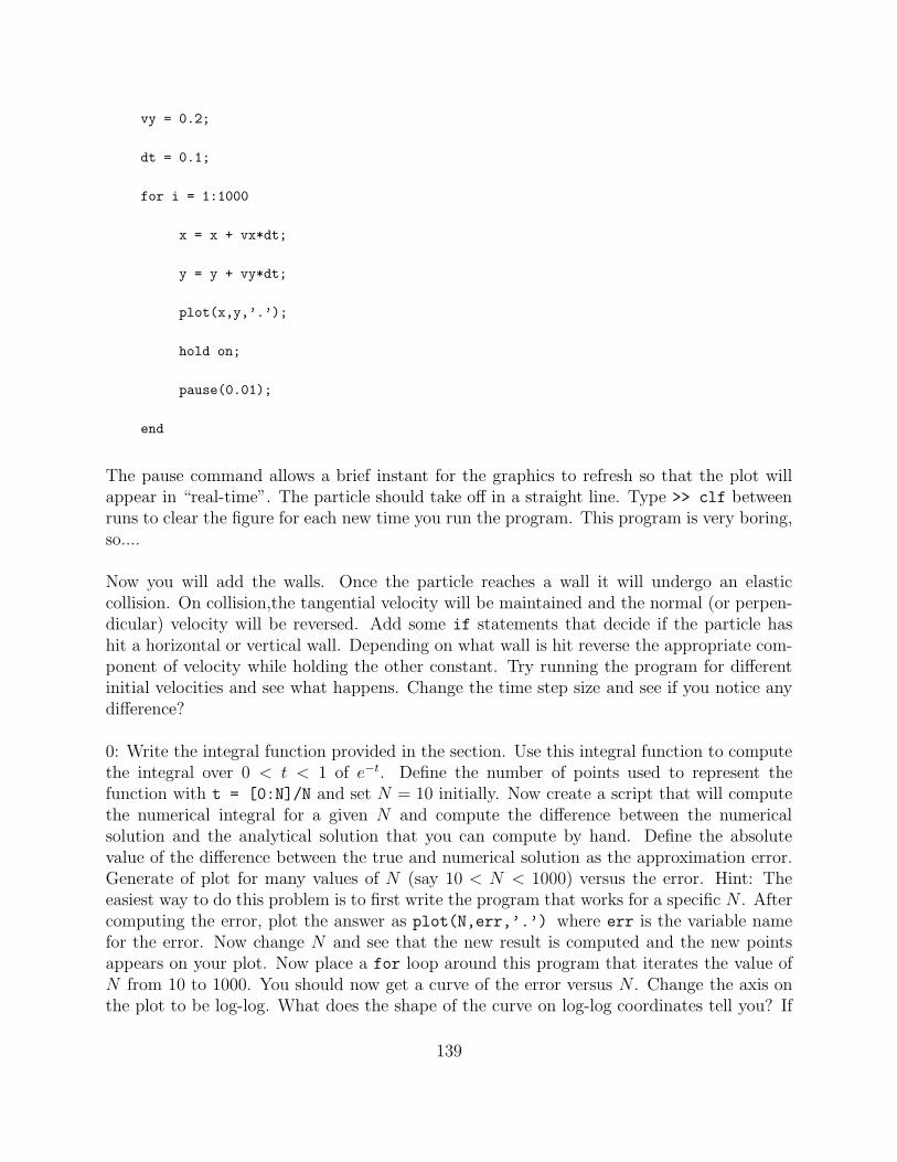
vy = 0.2;

dt = 0.1;

for i = 1:1000

x = x + vx*dt;

y = y + vy*dt;

plot(x,y,’.’);

hold on;

pause(0.01);

end

The pause command allows a brief instant for the graphics to refresh so that the plot willappear in “real-time”. The particle should take off in a straight line. Type >> clf betweenruns to clear the figure for each new time you run the program. This program is very boring,so....

Now you will add the walls. Once the particle reaches a wall it will undergo an elasticcollision. On collision,the tangential velocity will be maintained and the normal (or perpen-dicular) velocity will be reversed. Add some if statements that decide if the particle hashit a horizontal or vertical wall. Depending on what wall is hit reverse the appropriate com-ponent of velocity while holding the other constant. Try running the program for differentinitial velocities and see what happens. Change the time step size and see if you notice anydifference?

0: Write the integral function provided in the section. Use this integral function to computethe integral over 0 < t < 1 of e−t. Define the number of points used to represent thefunction with t = [0:N]/N and set N = 10 initially. Now create a script that will computethe numerical integral for a given N and compute the difference between the numericalsolution and the analytical solution that you can compute by hand. Define the absolutevalue of the difference between the true and numerical solution as the approximation error.Generate of plot for many values of N (say 10 < N < 1000) versus the error. Hint: Theeasiest way to do this problem is to first write the program that works for a specific N . Aftercomputing the error, plot the answer as plot(N,err,’.’) where err is the variable namefor the error. Now change N and see that the new result is computed and the new pointsappears on your plot. Now place a for loop around this program that iterates the value ofN from 10 to 1000. You should now get a curve of the error versus N . Change the axis onthe plot to be log-log. What does the shape of the curve on log-log coordinates tell you? If

139

you double the number of points, what happens to the error.

0: In the early 1800’s an English botanist, Robert Brown, observed that pollen grains con-tained in a drop of water wiggled about in a jagged, random path. Later this behavior wasattributed to molecular fluctuations in the water. Water molecules impinge on the smallparticle causing random forces acting in random directions. If the particle is small enoughthen the particle will move about in response to these random forces.

A simple model of Brownian motion in two dimensions is as follows: Take a particle andplace it at the origin x = y = 0. Use a for loop to take steps in time. At each time stepadd a normally distributed (i.e. bell-curve) random number to the horizontal and verticalcoordinate. Plot the position of the particle at each step. The MATLAB command randn(1)

will generate a single random number. The command plot(x,y,’.’) will plot a single datapoint and the command hold on will hold the graphics “on” so that the next iteration willplot the point on the same graph.

Write a program that plots the path (in x-y space) of one particle over 10,000 iterations.Try running the program a few times and see what patterns you develop. You will noticethat each run will look very unique. Type >> clf between runs to clear the figure for eachnew time you run the program.

0: In order to do this problem, we need an image to process. Any image will do. Youcan check the file types that are supported by the function imread. Most common formatssuch as tiff and jpeg are supported. The function imread will import the image file intothe MATLAB workspace. If the image is color you will get a three dimensional array, two-dimensions for the picture and the third for RGB scale. If the original picture is gray-scalethen you will get a two-dimensional array The format for the numbers is unit8 which is notsuitable for mathematics, so we transform the image data type to a default for numbers,double. The command imagesc is useful for plotting images; the function performs selfscaling. Try the following sequence of commands

>> A = imread(’picture.jpg’);

>> image(A);

>> whos


A 450x600x3 810000 uint8 array


140

>> A = double(A(:,:,1)); %% take only one color level.

>> whos




>> imagesc(A); %% this will look a little funny since we are not decoding the color

Now you can manipulate the two-dimensional array, A. Write a program that applies a“binary” threshold filter to the image data array. The threshold filter sets some value andeverything above the filter is “on” and everything below is “off”. Have your program workas a function. The input value is a two-dimensional data array. The program should findthe average value of the input image and use that value as the threshold. The new imageshould be the same size as the input and consist of one and zero depending on if you areabove or below the threshold. The output of the program should be the new image data file.Plot the output using imagesc. Try plotting the element by element multiplication of theinput and output data arrays.

141

0 0.2 0.4 0.6 0.8 1 1.2 1.4 1.6 1.8−20

0

20

40

time (s)

vel (

cm/s

)Max x−vel 38.69 Max y−vel 12.02

0.4 0.6 0.8 1 1.2 1.4 1.6 1.8 210

20

30

40

time (s)

x−ve

l (cm

/s)

STD 4.4 Mean 24

0.4 0.6 0.8 1 1.2 1.4 1.6 1.8 2−20

−10

0

10

20

time (s)

y−ve

l (cm

/s)

STD 3.3 Mean −0.095

Figure 5: The resulting figure from the program created to analyze the data from the hot-wireanemometer.

142

Documents

Commentary on the DSP First Labsweb.mit.edu/jrising/Public/dsplabs.pdf · Commentary on the DSP First Labs, In which is discussed the concerns of such labs as might be found in the