Embed Size (px)
Citation preview

Combining the FDTD Algorithm with Signal Processing Techniques for Performance Enhancement
Kapil Sharma, K. Panayappan, Ravi K. Arya and R. Mittra
EMC Lab, The Pennsylvania State University [email protected]

Conventional FDTD algorithm § Time domain numerical convergence (e.g., below 30 dB levell is used as the termination criterion
for conventional FDTD algorithm. § The termination criterion used in conventional FDTD results in high computational cost when a given problem is solved for low frequencies, or when high-Q structures and dispersive dielectric medium are involved.
0 100 200 300 400 500 600 700 800 900 1000-0.35
-0.3
-0.25
-0.2
-0.15
-0.1
-0.05
0
Frequency in MHz
Mag
nitu
de in
dB
Variation of S12
DC Gaussian
Frequency 10 MHz 1 MHz 1 Hz
Time Steps 6.9582e+005 6.9582e+006 6.9582e+012

Proposed Solution - Efficient FDTD algorithm
§ The proposed efficient FDTD algorithm utilizes signal processing techniques to check convergence in the frequency domain (as opposed to time domain), and thus differs from the conventional FDTD algorithm.
§ First, we wait until the first overshoot of the time signature has occurred § Then we compute the DFT of these samples at the lowest frequency of interest at the
end of every 100 time steps. § The FDTD algorithm is terminated when the difference between the successive DFT
values becomes negligible.

0 500 1000 1500 2000 2500 3000 3500 4000 4500 50000
0.005
0.01
0.015
0.02
0.025
0.03
0.035
Frequency in MHz
Mag
nitu
de
Variation of S13
DC Gaussian
Proposed Solution – Low Frequency Processing
§ Region 3: High frequency regime - Use DC Gaussian pulse results. § Region 1: Low frequency regime - Use the proposed method. § Region 2: Validation region – Use the Single Frequency results in this region to
validate the smoothed DC Gaussian results.
1 2 3
Frequency Definitions: fL - User Input f1 - 500 – 1000 MHz f2 - 2 f1 /3 f1 fH - User Input
High frequency regime
Validation Region
Low frequency regime
fL f1 f2 fH

Proposed Solution – Low Frequency Processing (Contd.)
§ Smooth the DC Gaussian Results. § Fit the curve from fL to f1 with the DC values, using a quadratic curve. The choice of
f1 can be fine tuned based on the quality of the resulting fit. § Validate the smoothed “DC Gaussian” results in region 2 by comparing them with
those generated by “Single Frequency” simulations at a few points (typically 2 or 3).
Frequency Definitions: fL - User Input f1 - 500 – 1000 MHz f2 - 2 f1 /3 f1 fH - User Input
0 500 1000 1500 2000 2500 3000 3500 4000 4500 50000
0.005
0.01
0.015
0.02
0.025
0.03
0.035
Frequency in MHz
Mag
nitu
de
Variation of S13
DC Gaussian
1 2 3
High frequency regime
Validation Region
Low frequency regime
fL f1 f2 fH

RF Filter
X Z
Y
f @ 0 Hz to 1.5 GHz
εr = 2 1 mm
Y X
Z
0 500 1000 1500-50
-40
-30
-20
-10
0
10
Frequency in MHz
Mag
nitu
de in
dB
Variation of S12
DC GaussianSingle FrequencyUniversal GEMSFEKO
0 500 1000 1500-45
-40
-35
-30
-25
-20
-15
-10
-5
0
Frequency in MHz
Mag
nitu
de in
dB
Variation of S11
DC GaussianSingle FrequencyUniversal GEMSFEKO

Connector f @ 10 MHz to 1.5 GHz
1 3
2
4

Connector (Contd.)
0 500 1000 1500-50
-45
-40
-35
-30
-25
-20
-15
-10
Frequency in MHz
Mag
nitu
de in
dB
Variation of S11
DC GaussianSingle FreqeuncyUniversal GEMS
0 500 1000 1500-0.5
-0.45
-0.4
-0.35
-0.3
-0.25
-0.2
-0.15
-0.1
-0.05
0
Frequency in MHz
Mag
nitu
de in
dB
Variation of S12
DC GaussianSingle FreqeuncyUniversal GEMS
0 500 1000 1500-60
-55
-50
-45
-40
-35
-30
Frequency in MHz
Mag
nitu
de in
dB
Variation of S13
DC GaussianSingle FreqeuncyUniversal GEMS
0 500 1000 1500-60
-55
-50
-45
-40
-35
-30
-25
-20
Frequency in MHz
Mag
nitu
de in
dB
Variation of S14
DC GaussianSingle FreqeuncyUniversal GEMS
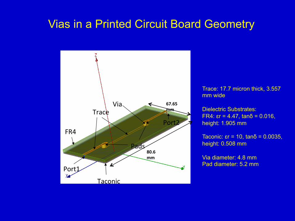
Vias in a Printed Circuit Board Geometry
Trace: 17.7 micron thick, 3.557 mm wide Dielectric Substrates: FR4: ԑr = 4.47, tanδ = 0.016, height: 1.905 mm Taconic: ԑr = 10, tanδ = 0.0035, height: 0.508 mm Via diameter: 4.8 mm Pad diameter: 5.2 mm
Trace Via
Pads
Port1
Port2 FR4
Taconic
80.6 mm
67.65 mm

Comparison of simulated return loss (S11)
0.5 1 1.5 2 2.5 3 3.5 4 4.5 5-45
-40
-35
-30
-25
-20
-15
-10
-5
0
Frequency (GHz)
S11
(dB)
S11 Comparison
S11: Conventional FDTDS11: FDTD combined with signal processingS11: Commercial FEM Solver
Same accuracy is obtained in return loss (S11) using conventional FDTD and efficient FDTD algorithms. Results obtained using FDTD compare well against those obtained using commercial FEM solver.

Comparison of computational resources utilized
Use of signal processing along with conventional FDTD algorithm reduces the computation time as compared to conventional FDTD algorithm. Also, computational resources utilized by both FDTD algorithms are less than those utilized by the commercial FEM solver.

Conclusions
• An efficient FDTD algorithm has been proposed in this work, which utilizes signal processing techniques to reduce the overall computational cost.
• Results for different test examples demonstrated show that the FDTD algorithm used along with signal processing reduces computational cost while maintaining the accuracy of the results. Cost savings vary depending on the nature of the problem and the frequency range of interest. The savings can range from a few percent to a large factor.
References
• [1] Kane S. Yee, “Numerical Solution of Initial Boundary Value Problems Involving Maxwell’s Equations in Isotropic Media,” IEEE Trans. On Antennas and Propagation, vol.14, no.3, pp. 302-307, May 1966.
• [2] Wenhua Yu, Xiaoling Yang, Yongjun Liu and Raj Mittra, Electromagnetic Simulation Techniques Based on the FDTD Method, John Wiley & Sons, Inc., 2009.
• [3] R. Mittra, Computer Techniques for Electromagnetics, New York: Hemisphere Publication Corporation, 1987.
• [4] Kadappan Panayappan, Novel Frequency Domain Techniques and Advances in Finite Difference Time Domain (FDTD) Method for Efficient Solution of Multiscale Electromagnetic Problems, PhD Dissertation, The Pennsylvania State University, 2013.

Thank You
Questions ?