Embed Size (px)
Citation preview

Combined Analysis of Electricity and Heat
Networks
Xuezhi Liu
Institute of Energy
Cardiff University
A thesis submitted for the degree of
Doctor of Philosophy
September, 2013

ii
Acknowledgment
This presented PhD thesis would not have been possible without the
numerous, continuous guidance and help from Prof. Nick Jenkins. I
appreciate his honesty and patience. His strong insights and professional
writing style illuminated me in many ways, which significantly improved
the thesis.
I would like to thank Dr. Jianzhong Wu for bringing me to this promising
ripe research area. I thank him for his enormous helpful guidance and
support in many ways.
I would like to thank Dr. Audrius Bagdanavicius for the numerous,
important, constructive and fruitful discussions in technical details
throughout my entire PhD journey.
I would like to thank Dr. Janaka Ekanayake for his kind support and
suggestions.
I would like to thank Marc Rees for constant discussions in how to
present the work clearly.
I would like to thank people in our group: Lee Thomas for helping to
design the electrical network of the case study, Daniel Oluwole Adeuyi
for improving the writing of some sentences, Bieshoy Awad for
introducing district heating networks, and Brian Drysdale for reading
Chapter 1. I also would like to thank Meysam Qadrdan and Modassar
Chaudry for the discussions in the Energy Infrastructure group weekly
meeting and the many friends made within the Institute of Energy.
I would like to thank Xi Hu at Oxford for improving the writing of Chapter
1, Xiaobo Hu, at China Electric Power Research Institute who visited
Cardiff, for discussing the model of combined analysis, Chao Long at
Glasgow for discussing electrical power flow calculation of the case
study, and Brian Boyle at Cardiff for discussing the writing of Chapter 2.

iii
I would like to acknowledge the EPSRC for their financial support
through the HiDEF project and organising training and meetings. I also
would like to thank the support received from Cardiff University,
especially the Research Students’ Skills Development Programme
(RSSDP) provided by the University Graduate College; and the IT office
and the research office in School of Engineering.
Finally, I would like to express my deepest appreciation to my parents
and sister for their unconditional love and continuous support.

Declaration
This work has not previously been accepted in substance for any degree
and is not concurrently submitted in candidature for any degree.
Signed ……………………..(candidate) Date ……………………….
This thesis is being submitted in partial fulfilment of the requirements for
the degree of PhD.
Signed ……………………..(candidate) Date ……………………….
This thesis is the result of my own independent work/investigation,
except where otherwise stated. Other sources are acknowledged by
explicit references.
Signed ……………………..(candidate) Date ……………………….
I hereby give consent for my thesis, if accepted, to be available for
photocopying and for inter-library loan, and for the title and summary to
be made available to outside organisations.
Signed …………………….. (candidate) Date ……………………….

Abstract
The use of Combined Heat and Power (CHP) units, heat pumps and
electric boilers increases the linkages between electricity and heat
networks. In this thesis, a combined analysis was developed to
investigate the performance of electricity and heat networks as an
integrated whole. This was based on a model of electrical power flow
and hydraulic and thermal circuits together with their coupling
components (CHP units, heat pumps, electric boilers and circulation
pumps). The flows of energy between the electricity and heat networks
through the coupling components were taken into account.
In the combined analysis, two calculation techniques were developed.
These were the decomposed and integrated electrical-hydraulic-thermal
calculation techniques in the forms of the power flow and simple optimal
dispatch. Using the combined analysis, the variables of the electrical and
heat networks were calculated. The results of the decomposed and
integrated calculations were very close. The comparison showed that the
integrated calculation requires fewer iterations than the decomposed
calculation.
A case study of Barry Island electricity and district heating networks was
conducted. The case study examined how both electrical and heat
demands in a self-sufficient system (no interconnection with external
systems) were met using CHP units. A solution was demonstrated to
deliver the electrical and heat energy from the CHP units to the
consumers through electrical and heat networks.
The combined analysis can be used for the design and operation of
integrated heat and electricity systems for energy supply to buildings.
This will increase the flexibility of the electricity and heat supply systems
for facilitating the integration of intermittent renewable energy.

Contents
Combined Analysis of Electricity and Heat Networks ......................... i
Acknowledgment ................................................................................... ii
Declaration… ......................................................................................... iv
Abstract………. ....................................................................................... v
Contents……….. .................................................................................... vi
List of Figures ........................................................................................ x
List of Tables ....................................................................................... xiii
Nomenclature ....................................................................................... xv
Variables ............................................................................................. xv
Subscripts and Superscripts .............................................................. xvii
Chapter 1 - Introduction ........................................................................ 1
1.1 Background .................................................................................... 1
1.2 Electricity and District Heating Networks ........................................ 3
1.2.1 Electricity Networks .................................................................. 3
1.2.2 District Heating Networks ......................................................... 4
1.3 Interdependencies between Electricity and Heat Networks ............ 5
1.4 Modelling Review ............................................................................ 7
1.5 Research Objective ........................................................................ 9
1.6 Thesis Structure ............................................................................ 10
Chapter 2 - Analysis of District Heating Networks ............................ 11
2.1 Hydraulic Model ............................................................................ 12
2.1.1 Continuity of Flow ................................................................... 13
2.1.2 Loop Pressure Equation ......................................................... 14
2.1.3 Head Loss Equation ............................................................... 15

Contents
vii
2.2 Solution of the Hydraulic Model .................................................... 16
2.2.1 Newton-Raphson Method ....................................................... 16
2.2.2 Radial District Heating Network .............................................. 18
2.2.3 Meshed District Heating Network ........................................... 18
2.3 Thermal Model .............................................................................. 23
2.4 Solution of the Thermal Model ...................................................... 24
2.4.1 Supply Temperature Calculation ............................................ 25
2.4.2 Return Temperature Calculation ............................................ 28
2.5 Hydraulic-Thermal Model .............................................................. 31
2.5.1 Introduction ............................................................................. 31
2.5.2 Decomposed Hydraulic-Thermal Calculation ......................... 32
2.5.3 Integrated Hydraulic-Thermal Calculation .............................. 36
2.6 Summary ...................................................................................... 43
Chapter 3 - Combined Analysis of Electricity and Heat Networks .. 45
3.1 Introduction ................................................................................... 45
3.1.1 Combined Electricity and District Heating Networks ............... 45
3.1.2 Known Variables and Unknown Variables .............................. 50
3.1.3 Analogues of Electrical and Thermal Power Flows ................ 51
3.2 Coupling Components Model ....................................................... 52
3.2.1 CHP Units ............................................................................... 52
3.2.2 Heat Pumps ............................................................................ 56
3.2.3 Electric Boilers ........................................................................ 56
3.2.4 Circulation Pumps .................................................................. 57
3.2.5 Combined Coupling Components ........................................... 57
3.3 Electrical Power Flow Analysis ..................................................... 59
3.4 Combined Analysis ....................................................................... 61
3.4.1 Decomposed Electrical-Hydraulic-Thermal Calculation .......... 63

Contents
viii
3.4.2 Integrated Electrical-Hydraulic-Thermal Calculation ............... 68
3.5 Examples ...................................................................................... 72
3.5.1 Decomposed Electrical-Hydraulic-Thermal Calculation .......... 72
3.5.2 Integrated Electrical-Hydraulic-Thermal Calculation ............... 86
3.5.3 Comparison of Two Calculation Techniques .......................... 92
3.6 Summary ...................................................................................... 94
Chapter 4 - Case Study ........................................................................ 96
4.1 Introduction ................................................................................... 96
4.2 Network Description ...................................................................... 97
4.2.1 Electricity Network .................................................................. 99
4.2.2 Heat Network ........................................................................ 101
4.2.3 CHP Units ............................................................................. 102
4.3 Calculations ................................................................................ 103
4.4 Results ........................................................................................ 105
4.5 Convergence Characteristics ...................................................... 109
4.6 Optimal Dispatch of Electricity Generation ................................. 110
4.7 Summary .................................................................................... 115
Chapter 5 - Conclusions .................................................................... 117
5.1 Conclusions ................................................................................ 117
5.1.1 Analysis of District Heating Networks ................................... 117
5.1.2 Combined Analysis of Electricity and Heat Networks ........... 119
5.1.3 Case Study ........................................................................... 120
5.2 Contributions of the Thesis ......................................................... 121
5.3 Future Work ................................................................................ 122
Reference……… ................................................................................. 123
Appendix A - Hydraulic Calculation Methods .................................. 129
A1 A Simple Example .................................................................... 129

Contents
ix
A2 Solutions ................................................................................. 131
A2.1 h-equations using the Hardy-Cross method ..................... 131
A2.2 -equations using the Newton-Raphson method .......... 132
A2.3 -equations using the Hardy-Cross method ................. 133
A3 A Complicated Example .......................................................... 135
A3.1 -equations using the Newton-Raphson method .......... 137
A3.2 -equations using the Hardy-Cross method ................. 137
A4 Summary .................................................................................. 139
Appendix B - Derivation of the Temperature Drop Equation ......... 140
Appendix C - Data for the Example Networks ................................. 142
Appendix D - Pipe Parameters for the Case Study ......................... 144
Appendix E - Network Incidence Matrix for the Case Study .......... 145
Appendix F - Results Compared to SINCAL and IPSA for the Case
Study ............................................................................ 147

List of Figures
Figure 1.1: 2011 UK Greenhouse gas emissions by source sector ......... 1
Figure 1.2: Electrical distribution network ................................................ 3
Figure 1.3: A simplified district heating network with two heat production
units ................................................................................................... 4
Figure 1.4: Global deployment of heating technologies in the IEA
scenario, 2007/2010 to 2050 (GWth) ................................................. 6
Figure 1.5: Research Framework ............................................................. 9
Figure 2.1: A district heating network with a loop ................................... 12
Figure 2.2: A radial district heating network ........................................... 18
Figure 2.3: Result of the mass flow rate within pipe 3 from SINCAL ...... 22
Figure 2.4: Temperatures associated with each node ........................... 23
Figure 2.5: A simple district heating network with a loop ....................... 25
Figure 2.6: Flowchart of the supply temperature calculation .................. 27
Figure 2.7: Flowchart of the return temperature calculation ................... 30
Figure 2.8: Structure of the decomposed hydraulic-thermal calculation
with specified nodal heat power ...................................................... 32
Figure 2.9: Flowchart of the decomposed hydraulic-thermal calculation
with specified nodal power .............................................................. 33
Figure 2.10: A district heating network with a loop ................................. 34
Figure 2.11: Result of the supply temperature at the load 1 from SINCAL
........................................................................................................ 36
Figure 2.12: Derivation of the system of equations for the integrated
hydraulic-thermal calculation ........................................................... 37
Figure 2.13: Structure of the integrated hydraulic-thermal calculation with
specified nodal heat power .............................................................. 38
Figure 3.1: Schematic diagram of the combined electricity and district
heating networks in islanded mode ................................................. 46
List of Figures
xi
Figure 3.2: Energy flow of a CHP and heat pump composite supply
system (picture sources: ARUP DENet and GE’s Jenbacher Gas
Engines) .......................................................................................... 46
Figure 3.3: Schematic diagram of the combined electricity and district
heating networks in grid-connected mode ....................................... 47
Figure 3.4: Schematics of the decomposed electrical-hydraulic-thermal
calculation (a.i) in grid-connected mode and (a.ii) islanded mode and
(b) the integrated electrical-hydraulic-thermal calculation ............... 49
Figure 3.5: Structure of the integrated electrical-hydraulic-thermal
calculation technique ....................................................................... 50
Figure 3.6: Schematic of condensing steam turbines with extraction ..... 54
Figure 3.7: The relation between heat and electrical power generation of
CHP units: (a) gas turbines or internal combustion engines and (b)
extraction steam turbines ................................................................ 55
Figure 3.8: A CHP and heat pump composite supply system ................ 58
Figure 3.9: Flowchart of the decomposed electrical-hydraulic-thermal
calculation ....................................................................................... 65
Figure 3.10: Flowchart of the integrated electrical-hydraulic-thermal
calculation ....................................................................................... 68
Figure 3.11: A simple grid-connected electricity network and a district
heating network ............................................................................... 72
Figure 3.12: A simple islanded electricity network and a district heating
network ............................................................................................ 81
Figure 3.13: Procedure to calculate the electrical and heat power from
both Source 1 and Source 2 that link electricity and heat networks 83
Figure 3.14: Electrical and heat power supplied from two sources ........ 86
Figure 3.15: Procedure to calculate the electrical and heat power from
both Source 1 and Source 2 that link electricity and heat networks 90
Figure 3.16: Convergence characteristics of the decomposed and
integrated electrical-hydraulic-thermal calculations ......................... 93
Figure 4.1: Linkages between electricity and district heating networks . 96
Figure 4.2: Schematic diagram of the electricity and district heating
networks of the Barry Island case study .......................................... 98

List of Figures
xii
Figure 4.3: Schematic diagram of the electric power distribution network
of the Barry Island case study ......................................................... 99
Figure 4.4: Schematic diagram of the heat network of the Barry Island
case study ..................................................................................... 101
Figure 4.5: Heat and electrical power supplied from three sources ..... 106
Figure 4.6: Results of the pipe mass flow rates (kg/s) in a flow route .. 106
Figure 4.7: Results of the supply and return temperatures of the nodes in
a flow route .................................................................................... 107
Figure 4.8: Results of the voltage magnitude and voltage angle at each
busbar ........................................................................................... 108
Figure 4.9: Convergence characteristics of the decomposed and
integrated calculations ................................................................... 109
Figure 4.10: Illustration of optimal dispatch for combined electrical and
heat power ..................................................................................... 111
Figure 4.11: Flowchart of the decomposed electrical-hydraulic-thermal
calculation ..................................................................................... 113
Figure 4.12: Heat and electrical power supplied from three sources ... 115
Figure A.1: A pipe network with a loop ................................................ 129
Figure A.2: A district heating network with multi-loops ........................ 135

List of Tables
Table 2.1: Analogy of rules in electrical network and district heating
network ............................................................................................ 12
Table 2.2: Three systems of equations in hydraulic model .................... 19
Table 2.3: Results of the decomposed and integrated hydraulic-thermal
calculations ...................................................................................... 43
Table 3.1: Known and unknown variables of the electricity and heat
networks and the coupling components .......................................... 51
Table 3.2: Analogues of the known variables in electricity and heat
networks .......................................................................................... 52
Table 3.3: Analogues of busbar and node types in electrical and thermal
power flows ..................................................................................... 52
Table 3.4: Known variables and unknown variables of electricity and heat
networks .......................................................................................... 73
Table 3.5: Known variables for the example networks ........................... 74
Table 3.6: Results of the decomposed electrical-hydraulic-thermal
calculation ....................................................................................... 80
Table 3.7: Known variables and unknown variables of electricity and heat
networks .......................................................................................... 81
Table 3.8: Number of iterations in the hydraulic and thermal and
electrical models .............................................................................. 84
Table 3.9: Results of the decomposed electrical-hydraulic-thermal
calculation ....................................................................................... 85
Table 3.10: Results of the integrated electrical-hydraulic-thermal
calculation ....................................................................................... 89
Table 3.11: Results of the integrated electrical-hydraulic-thermal
calculation ....................................................................................... 91
Table 3.12: Differences of the solutions between decomposed and
integrated calculations ..................................................................... 92
Table 4.1: Heat and electrical power from three sources ..................... 103

List of Tables
xiv
Table 4.2: Number of the state variables for the case study ................ 103
Table 4.3: Heat and electrical power from three sources ..................... 110

Nomenclature
Variables
V Voltage (V)
θ Voltage angle (rad)
P Electrical real power (MWe)
Q Electrical reactive power (MVar)
S Electrical complex power (MVA)
Φ Heat power (MWth)
Mass flow rate within each pipe (kg/s)
Injected mass flow rate at each node (kg/s)
Ts Supply temperature at a node in the supply network (°C)
To Return temperature at the outlet of a node before mixing in
the return network (°C)
Tr Return temperature at a node after mixing in the return
network (°C)
Ta Ambient temperature (°C)
T's Difference between Ts and Ta
T'r Difference between Tr and Ta
Tstart Temperature at the start node of a pipe (°C)
Tend Temperature at the end node of a pipe (°C)
Head loss (m) within a pipe
H Head level (m)
Hc Minimum allowable head differential (m)
Hp Pump head (m)
A Network incidence matrix
B Loop incidence matrix
Cp Specific heat of water (J/(kg·K))
λ Overall heat transfer coefficient per unit length (W/(m·K))
cm Heat to power ratio
Equivalent heat-to-power ratio of a composite CHP and heat
pump system

Nomenclature
xvi
Z Z ratio that describes the trade-off between heat supplied to
site and electrical power
K Resistance coefficient of each pipe
L Pipe length (m)
D Pipe diameter (m)
ρ Water density (kg/m3)
g Gravitational acceleration (kg·m/s2).
f Friction factor
Re Reynolds number
ε Roughness of a pipe (m)
v Flow velocity (m/s)
μ Kinematic viscosity of water (m2/s).
J Jacobian matrix
ΔF Vector of mismatches
x Vector of unknown state variables
C Matrix of coefficients
b Column vector of solutions
PCHP Electrical power output of a CHP unit (MWe)
ΦCHP Useful heat output of a CHP unit (MWth)
Php Electrical power consumed from a heat pump (MWe)
Φhp Heat power supplied from a heat pump (MWth)
Pcon Electrical power generation of an extraction steam turbine
CHP unit in full condensing mode (MWe)
α Percentage of a fraction of electrical power from the CHP unit
modulated to drive the heat pump
Electrical efficiency of an extraction steam turbine CHP unit
in full condensing mode
Fin Fuel input rate (MW)
ηb Efficiency of an electric boiler
COP Coefficient of performance
ηp Efficiency of a circulation pump
Electrical power consumed (MWe) by a circulation pump
Mass flow rate (kg/s) through a criculation pump

Nomenclature
xvii
Consumed electrical power (MWe) by a circulation pump
A set which includes all the pipes in the critical route with the
largest pressure drop in a heat network
Y Admittance matrix
Real Real part of a complex expression
Imag Imaginary part of a complex expression
Fuel cost of Source i (£/h)
Incremental fuel cost (£/MWh)
nnode Number of nodes in heat networks
nload Number of loads in heat networks
nloop Number of loops in heat networks
npipe Number of pipes in heat networks
N Number of busbars in electricity networks
Subscripts and Superscripts
p pump
hp heat pump
b boiler
e electrical network
h heat network
sp specified
Chapter 1 - Introduction
1.1 Background
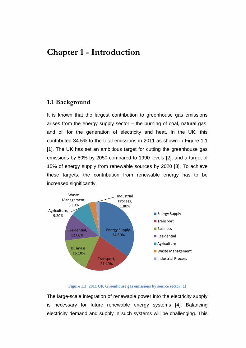
It is known that the largest contribution to greenhouse gas emissions
arises from the energy supply sector – the burning of coal, natural gas,
and oil for the generation of electricity and heat. In the UK, this
contributed 34.5% to the total emissions in 2011 as shown in Figure 1.1
[1]. The UK has set an ambitious target for cutting the greenhouse gas
emissions by 80% by 2050 compared to 1990 levels [2], and a target of
15% of energy supply from renewable sources by 2020 [3]. To achieve
these targets, the contribution from renewable energy has to be
increased significantly.
Figure 1.1: 2011 UK Greenhouse gas emissions by source sector [1]
The large-scale integration of renewable power into the electricity supply
is necessary for future renewable energy systems [4]. Balancing
electricity demand and supply in such systems will be challenging. This
Energy Supply, 34.50%
Transport, 21.40%
Business, 16.10%
Residential, 12.60%
Agriculture, 9.20%
Waste Management,
3.10%
Industrial Process, 1.80%
Energy Supply
Transport
Business
Residential
Agriculture
Waste Management
Industrial Process

Chapter 1 - Introduction
2
is because the output of renewables such as wind is intermittent and it is
not easy to modulate the output of renewables to follow a particular load
profile. Thus, the flexibility of energy supply system that can
accommodate intermittent renewables will become important.
The energy supply system is usually considered as individual sub-
systems with separate energy vectors (e.g. electricity, heat, gas and
hydrogen). In addition to electricity, heat is a major contributor to
greenhouse gas emissions. Almost half (44%) of the final energy
consumed in the UK is used to provide heat [5]. The Renewable Heat
Incentive (RHI) is a policy promoting renewable heat technologies, which
aims to encourage the uptake of renewable sources such as biomass
boilers, heat pumps and solar thermal systems [6].
In the present Smart Grid vision, the role of electricity is most prominent
with limited consideration of other energy networks. However, there is
much benefit to be gained by considering the energy system as an
integrated whole. Energy flows can be controlled, loads supplied from
alternative sources and so security of energy supply increased. The most
energy efficient operating regime can be determined and energy losses,
costs or gaseous emissions minimised. Independent planning and
operation of energy networks is unlikely to yield an overall optimum,
since synergies between the different energy vectors cannot be
exploited. Thus, an integration of energy systems is highly desirable [7].
One possibility to integrate electricity and heat networks is to use district
heating systems. Combined Heat and Power (CHP) units and boilers
connected to district heating systems and heat pumps act as linkages
between electricity and heat networks. These allow a coupling of the
electricity and heat networks, and make use of synergies of the two
networks for energy storage and the utilisation of distributed renewable
energy. The coupling components (CHP units, heat pumps, electric
boilers and circulation pumps) increase flexibility for equalising the
fluctuations from the renewable energy. Flexibility is achieved through
the optimisation of electric power consumption in heat pumps and supply
in CHP units. As the penetration of the coupling components increases,

Chapter 1 - Introduction
3
the interaction of electricity and heat networks becomes tighter and
modelling electricity and heat networks as a whole becomes increasingly
important.
1.2 Electricity and District Heating Networks
1.2.1 Electricity Networks
Transmission networks refer to the bulk transfer of power by high-voltage
links between central generation and load centres. Distribution networks,
on the other hand, describe the distribution of this power to consumers
by means of lower voltage networks (see Figure 1.2) [8]. Generators
usually produce voltages in the range 11-25kV, which is increased by
transformers to the main transmission voltage. At substations the
connections between the various components of the system, such as
lines and transformers, are made and the switching of these components
is carried out [8].
Distribution networks differ from transmission networks in several ways,
apart from their voltage levels. The number of branches -is much higher
in distribution networks and the general structure or topology is different.
A typical system consists of a step-down (e.g.33/11kV) on-load tap-
changing transformer at a bulk supply point feeding a number of circuits
which can vary in length from a few hundred metres to several
kilometres. A series of step-down three-phase transformers
(e.g.11kV/433V) are spaced along the route and from these are supplied
the consumer three-phase, four-wire networks which give 240V single-
phase supplies to houses and similar loads [8].
Grid
Local load
400V
Fixed-Tap
TransformerFeeder
Auto-Tap
Transformer
11kV33kV
Primary substation
Figure 1.2: Electrical distribution network [9]
Chapter 1 - Introduction
4
1.2.2 District Heating Networks
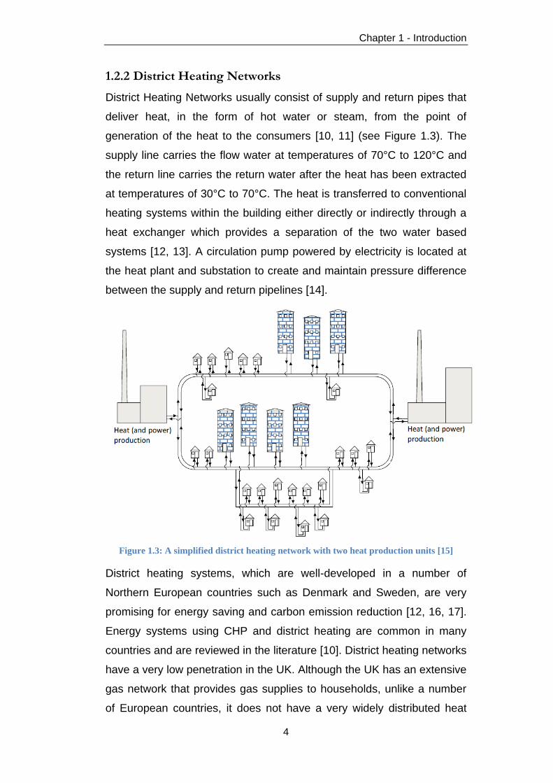
District Heating Networks usually consist of supply and return pipes that
deliver heat, in the form of hot water or steam, from the point of
generation of the heat to the consumers [10, 11] (see Figure 1.3). The
supply line carries the flow water at temperatures of 70°C to 120°C and
the return line carries the return water after the heat has been extracted
at temperatures of 30°C to 70°C. The heat is transferred to conventional
heating systems within the building either directly or indirectly through a
heat exchanger which provides a separation of the two water based
systems [12, 13]. A circulation pump powered by electricity is located at
the heat plant and substation to create and maintain pressure difference
between the supply and return pipelines [14].
Figure 1.3: A simplified district heating network with two heat production units [15]
District heating systems, which are well-developed in a number of
Northern European countries such as Denmark and Sweden, are very
promising for energy saving and carbon emission reduction [12, 16, 17].
Energy systems using CHP and district heating are common in many
countries and are reviewed in the literature [10]. District heating networks
have a very low penetration in the UK. Although the UK has an extensive
gas network that provides gas supplies to households, unlike a number
of European countries, it does not have a very widely distributed heat

Chapter 1 - Introduction
5
networks [18]. Nevertheless, some of the UK’s largest towns and cities
either already have district heating or are in the process of establishing
such schemes, examples include the city-wide heat networks in Sheffield
and Nottingham [10, 19].
Heat networks require significant deployment of new infrastructure and
therefore face a number of barriers to wide deployment. The low
penetration of district heating to date in the UK is partly due to the
relatively high cost of providing heat through district heating in
comparison with conventional gas or electric-based heating systems,
notably the cost of installing the pipes [12, 20-24]. A commercially viable
heat network requires a constant, large and consistent heat load, limiting
its suitability to specific locations [20, 21]. Besides, district heating
networks are complex projects, which have long lead‐in times and are
coupled with lengthy payback periods [21]. Furthermore, there is
currently no separately regulated market for heat in the UK, unlike
electricity or gas [20].
Although district heating networks face challenges, it offers many
benefits: increased energy efficiency; reduced fossil fuel consumption
and the ability to use local renewable energy resources [17, 25]. The
local heat sources are: low-grade heat generated from thermal power
stations, heat pumps, biomass CHP or boilers, solar thermal, industrial
waste heat and geothermal [5, 12, 22, 26-28]. District Heating can also
offer significant electricity demand-side management in relation to
intermittent wind output [29]. A number of Government White Papers
have cited district heating networks as an important enabler for the more
efficient utilisation of gas and the diffusion of renewable heating
technologies [30, 31].
1.3 Interdependencies between Electricity and Heat
Networks
CHP units, heat pumps, electric boilers and circulation pumps are the
coupling components between electricity and heat networks. These
coupling components allow flows of energy between electricity and heat

Chapter 1 - Introduction
6
networks. The CHP units generate electricity and heat simultaneously.
Heat pumps use a small quantity of electricity to leverage heat from the
surroundings to higher temperatures, using a compressor similar to a
refrigerator [22, 32]. Electric boilers convert electricity to heat directly.
Circulation pumps consume electricity to circulate water in the district
heating network.
Heat pumps and CHP/district heating are core heating technologies,
which could play a key role in meeting the UK and global heat demand in
an emissions constrained future [5, 28, 33, 34]. CHP can deliver energy
and carbon savings of up to 30% by reducing energy lost as waste heat
compared to separate electrical and heat power generation from the
same fuel [35]. The global deployment of heat pumps, solar thermal and
CHP in the IEA scenario to 2050 is shown in Figure 1.4 [36]. This data
indicates that the link between electricity and heat networks is
increasing. The larger the penetration of CHP/district heating and heat
pumps, the stronger the links between electricity and heat networks.
Figure 1.4: Global deployment of heating technologies in the IEA scenario, 2007/2010 to
2050 (GWth)
In an energy system with increased CHP/district heating and heat
pumps, the conversion to heat facilitates system operation and the use of
storages. For example, excess electricity can be converted to heat,
stored as heat in a tank or in the system when there is a surplus of
electricity from intermittent renewables [5, 26]. Using CHP with heat
accumulation to integrate intermittent renewable electricity supplies such
Chapter 1 - Introduction
7
as wind power into electricity systems has been demonstrated in various
countries [37]. In Germany, the demonstration project used biogas CHP
and hydropower to balance fluctuations in wind and solar power [38].
Pilot projects such as: feeding heat or hydrogen from weather-dependent
renewables into district heating or gas networks were launched [39, 40].
Thus, it becomes increasingly important to consider electricity and
heating systems as a whole to consider the synergy effects.
1.4 Modelling Review
Several conceptual approaches for modelling the integration of energy
systems have been published. Examples include energy hubs [7, 41],
multi-energy systems and distributed multi-generation [42-45],
community energy [43], smart energy systems [4, 46], and integrated
energy systems [10].
A generic framework for steady-state and optimisation of energy systems
is investigated by Geidl & Andersson [41]. The coupling between multiple
energy carriers are modelled by the use of energy hubs [47]. In the
modelling of energy hubs [41], electricity, natural gas, and district heat
input powers are converted to electricity and heat output powers through
an efficiency coupling matrix. Smart multi-energy systems were
described by Mancarella et al [42, 48, 49]. In multi-energy systems,
coupling of electricity, heat/cooling and gas networks through distribution
infrastructure takes place through various distributed technologies such
as CHP, micro-CHP, heat pump, solar thermal, photovoltaic, storage and
heat networks. In a community energy scheme [47], a transformer
substation in the electrical power system links the gas network and a
local heat network on the community scale, with sources installed at this
substation. Low temperature heat networks compatible with waste heat
from CHP, electric or engine driven heat pumps, or solar thermal was
used. Integrated energy systems focusing on the role of CHP and district
heating were described by the CHPA [10].
Methods have been developed to investigate combined electricity and
natural gas networks [7, 50-54], in which gas turbine generators provide

Chapter 1 - Introduction
8
the linkage between gas and electricity networks. A general approach
was described to execute a single gas and power flow analysis in a
unified framework based on the Newton-Raphson formulation [53]. There
have been a few studies that have investigated combined electricity and
heat networks, e.g. the energy hub model [7], the energy interconnector
model [55] and an integrated optimal power flow for electricity and heat
networks [56]. The simultaneous transmission of heat, electricity, and
chemical energy in one single device was modelled [55]. The integration
of technical design, green house gas emissions analysis and financial
analysis models for integrated community energy systems was modelled
by Rees [57, 58]. In these models the electrical, thermal and gas power
flows were calculated independently and linked through generating units.
The role of the coupling components (CHP units, heat pumps and
electric boilers) was investigated, i.e., a strategy [59], the economic value
[60], a technical approach [61, 62], and the impact of future heat demand
[63]. It is concluded that the increased diversity of heat delivery – with
gas, heat networks and electric heating all playing major roles, may
facilitate the difficult move towards a decarbonised future [64-66].
For individual heat network calculation, PSS SINCAL Heating [67] is a
commercial software for planning large networks. Using the Hardy-Cross
method, the simulation program can determine the operating points in
any number of meshed networks.
The Hardy-Cross method dealt with one loop at a time. The Newton-
Raphson method considered all loops simultaneously [11]. The Newton-
Raphson method was used to solve the electrical power flow. For the
sake of combining with the thermal model and further combining with the
electrical power flow, the Newton-Raphson method was used to solve
the hydraulic equations. Consistently, the Newton-Raphson method was
chosen to solve a unified formulation of the hydraulic-thermal equations
and the electrical power flow equations in this thesis.
Chapter 1 - Introduction
9
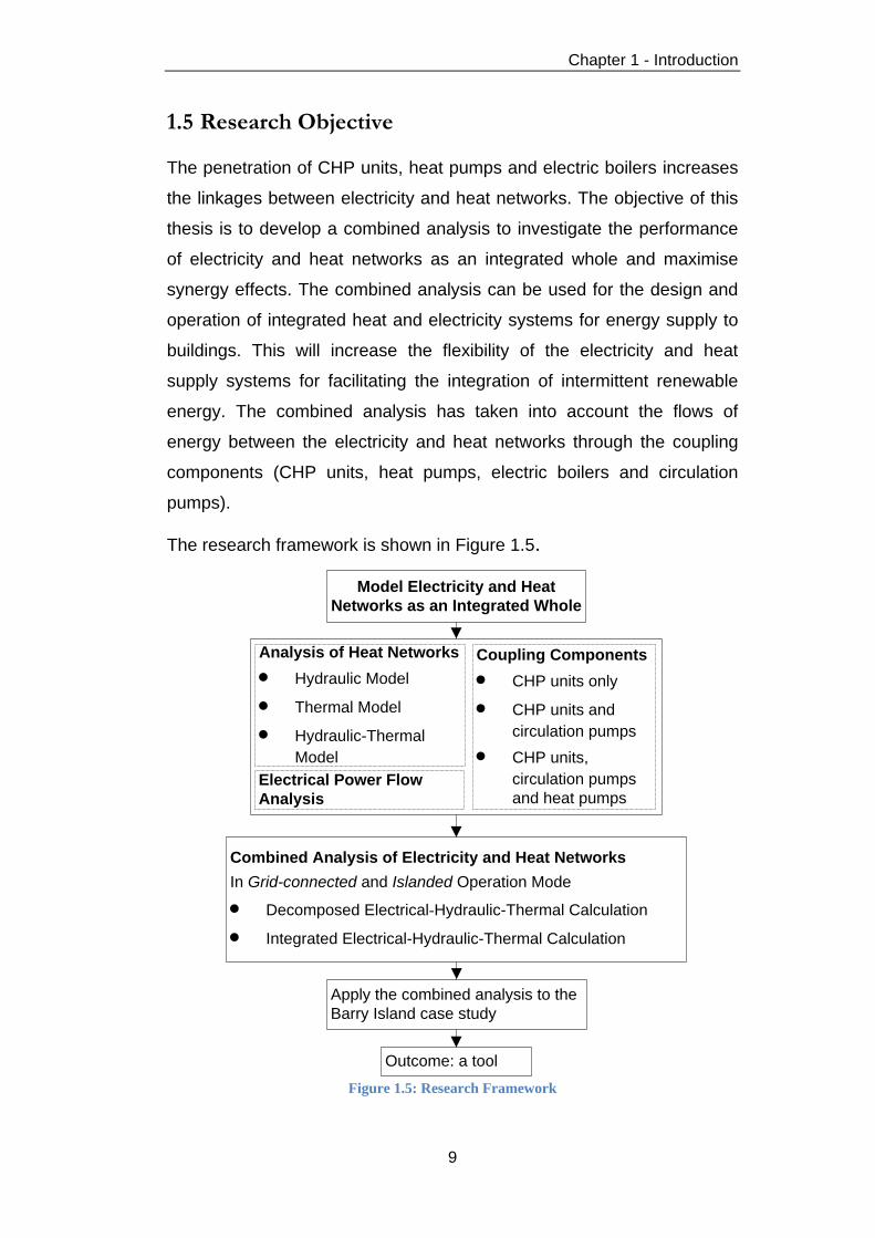
1.5 Research Objective
The penetration of CHP units, heat pumps and electric boilers increases
the linkages between electricity and heat networks. The objective of this
thesis is to develop a combined analysis to investigate the performance
of electricity and heat networks as an integrated whole and maximise
synergy effects. The combined analysis can be used for the design and
operation of integrated heat and electricity systems for energy supply to
buildings. This will increase the flexibility of the electricity and heat
supply systems for facilitating the integration of intermittent renewable
energy. The combined analysis has taken into account the flows of
energy between the electricity and heat networks through the coupling
components (CHP units, heat pumps, electric boilers and circulation
pumps).
The research framework is shown in Figure 1.5.
Model Electricity and Heat
Networks as an Integrated Whole
Apply the combined analysis to the
Barry Island case study
Outcome: a tool
Combined Analysis of Electricity and Heat Networks
In Grid-connected and Islanded Operation Mode
· Decomposed Electrical-Hydraulic-Thermal Calculation
· Integrated Electrical-Hydraulic-Thermal Calculation
Analysis of Heat Networks
· Hydraulic Model
· Thermal Model
· Hydraulic-Thermal
Model
Coupling Components
· CHP units only
· CHP units and
circulation pumps
· CHP units,
circulation pumps
and heat pumpsElectrical Power Flow
Analysis
Figure 1.5: Research Framework

Chapter 1 - Introduction
10
1.6 Thesis Structure
The description of each chapter is as follows:
Chapter 1 presents the introduction.
Chapter 2 describes an analysis of district heating networks. A hydraulic-
thermal model (decomposed and integrated calculations) was developed
to investigate the performance of a district heating network.
Chapter 3 describes a combined analysis of electricity and heat
networks. Two calculation techniques (decomposed and integrated
electrical-hydraulic-thermal calculations) were developed. This is based
on a model of electrical power flow and hydraulic and thermal circuits
together with their coupling components.
In Chapter 4, a case study of Barry Island examined how both electrical
and heat demands in a self-sufficient system (no interconnection with
external systems) were met using CHP units.
Chapter 5 presents the conclusions drawn, the main findings and
recommendations for future work.

Chapter 2 - Analysis of District Heating
Networks
District Heating Networks usually consist of supply and return pipes that
deliver heat, in the form of hot water or steam, from the point of
generation of the heat to the end consumers [10, 11]. In a simulation of a
district heating network, the variables are: pressure and mass flow rates
in the hydraulic model; supply and return temperatures and heat power
in the thermal model. Hydraulic and thermal analysis is carried out to
determine the mass flow rates within each pipe and the supply and
return temperatures at each node. Usually, hydraulic analysis is carried
out before the thermal analysis [11, 67-69]. It is common to perform
hydraulic calculations using the Hardy-Cross or Newton-Raphson
method [11, 67-70]. The Hardy-Cross method considers each loop
independently and the Newton-Raphson method considers all loops
simultaneously [11]. The decomposed hydraulic and thermal analysis of
a pipe network using the Newton-Raphson method is described in the
literature [68].
According to the literature [11, 67, 71, 72], the source supply
temperatures and the load return temperatures are specified; the injected
mass flow rates or the heat power supplied or consumed at all the nodes
except one are specified. Based on these assumptions, an integrated
hydraulic-thermal model of district heating networks, the so-called
thermal power flow by the Newton-Raphson method was presented in
Chapter 2 - Analysis of District Heating Networks
12
this Chapter. In the hydraulic model, the network description is based on
a graph-theoretical method. In the thermal model, a matrix approach was
used.
2.1 Hydraulic Model
The modelling of a district heating network is similar to that of an
electrical network. For electrical network and district heating network, the
analogy of three basic rules is shown in Table 2.1. The first two laws
describe the linear algebraic constraints on branch current and voltage
(or flow and pipe pressure drop in a district heating network), that are
independent of the branch characteristics [11]. The description of the first
two laws based on the graph theoretical method is described in the
literature [73, 74].
Table 2.1: Analogy of rules in electrical network and district heating network
Electrical
network
Kirchhoff’s current
law
Kirchhoff’s voltage
law
Ohm’s law
District heating
network
Continuity of flow Loop pressure
equation
Head loss
equation
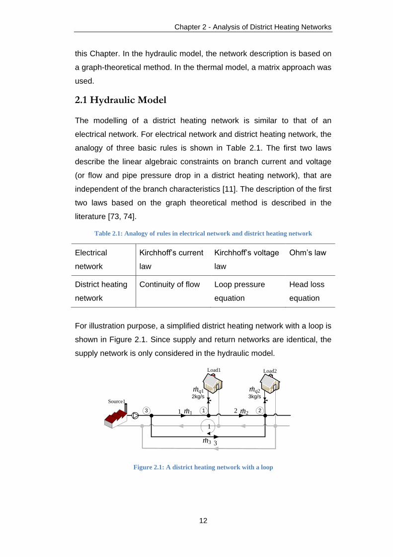
For illustration purpose, a simplified district heating network with a loop is
shown in Figure 2.1. Since supply and return networks are identical, the
supply network is only considered in the hydraulic model.
Load2
3
2kg/s 3kg/s
1 2
Source1
Load1
Load2
m1.
m2.
m3.
mq1 mq2
1
. .
13 2
Figure 2.1: A district heating network with a loop

Chapter 2 - Analysis of District Heating Networks
13
2.1.1 Continuity of Flow
The continuity of flow is expressed as: the mass flow that enters into a
node is equal to the mass flow that leaves the node plus the flow
consumption at the node, i.e.
(2.1)
where is the mass flow (kg/s) within each pipe; is the mass flow
(kg/s) through each node injected from a source or discharged to a load.
To describe the continuity of flow in a matrix form, the network incidence
matrix A with nnode = 3 rows and npipe = 3 columns is defined, where nnode
is the number of nodes and npipe is the number of pipes. Each element of
the matrix A describes [74]
+1, if the flow in a pipe comes into a node;
-1, if the flow in a pipe leaves a node;
0, if no connection from a pipe to a node.
is the vector of the mass flow (kg/s) through each node injected from
a source or discharged to a load. The element is positive if the flow
leaves the node and negative if it comes into the node.
For the network as shown in Figure 2.1, the network incidence matrix
and the nodal mass flow rates are
A =
(2.2)
For node 1, the continuity of flow is expressed as
or
(2.3)
1 2 3
1 1 -1 0
2 0 1 1
3 -1 0 -1
Node N
o.
Pipe No.

Chapter 2 - Analysis of District Heating Networks
14
Thus for the entire hydraulic network, the continuity of flow is expressed
as
(2.4)
The continuity of flow is applied at all nodes in a network, but one is
redundant because of it being linearly dependent on others and is
chosen arbitrarily for exclusion. Thus, in the following context, the
incidence matrix A of the network in Figure 2.1 is also written as
.
2.1.2 Loop Pressure Equation
Head loss is the pressure change in meters due to the pipe friction. The
loop pressure equation states that the sum of head losses around a
closed loop must equal to zero.
(2.5)
where is the head losses within a pipe, which is the difference of the
pressure head at the start and end nodes within a pipe.
The loop incidence matrix B with nloop = 1 rows and npipe = 3 columns is
defined, where nloop is the number of loops and npipe is the number of
pipes. Each element of the matrix B describes [74]
+1, if the flow in a pipe is the same direction as the definition;
-1, if the flow in a pipe is the opposite direction as the definition;
0, if a pipe is not part of the loop.
For the network as shown in Figure 2.1, the loop incidence matrix is
B =
(2.6)
1 2 3
1 1 1 -1
Pipe No.
Loop N
o.
Chapter 2 - Analysis of District Heating Networks
15
For loop 1, the equation (2.5) is expressed as
or
(2.7)
Thus correspondingly for the entire hydraulic network
(2.8)
where B is the loop incidence matrix that relates the loops to the pipes;
and hf is the vector of the head losses (m).
2.1.3 Head Loss Equation
The relation between the flow and the head losses along each pipe is
(2.9)
where K is the vector of the resistance coefficients of each pipe
calculated using equation (2.11). K generally depends largely on the
diameter of a pipe.
Hence, equation (2.8) is expressed as
(2.10)
where npipe is the number of pipes; i is the index of loops and j is the
index of pipes.
The resistance coefficient K of a pipe is calculated from the friction factor
f
(2.11)
where L is the pipe length (m); D is the pipe diameter (m); ρ is water
density (kg/m3); and g is gravitational acceleration (kg·m/s2).
The friction factor f generally depends on Reynolds number Re.
For laminar flow (Re<2320)

Chapter 2 - Analysis of District Heating Networks
16
(2.12)
For the more frequent turbulent flow (Re>4000), the friction factor f is
calculated by
(2.13)
where ε is the roughness of a pipe (m). The implicit equation (2.13) is
solved by the method adopted in the reference [75].
For 2300 < Re < 4000, linear interpolation is used.
Reynolds number Re is calculated from the flow velocity
(2.14)
where v is the flow velocity (m/s); μ is kinematic viscosity of water (m2/s).
The flow velocity is calculated from the mass flow rate
(2.15)
2.2 Solution of the Hydraulic Model
2.2.1 Newton-Raphson Method
The Newton-Raphson method [76, 77] is based on Taylor Series
expansion of f(x) about an operating point x0
(2.16)
Neglecting the higher order terms in equation (2.16) since the value of
is small enough and solving the linear approximation of
for gives
(2.17)

Chapter 2 - Analysis of District Heating Networks
17
The Newton-Raphson method replaces the old value x(i) by the new
value x(i+1) for the iterative solution as shown below
(2.18)
where i is the iteration time; and J is Jacobian matrix
(2.19)
Equation (2.18) is repeated until the mismatch is less than a
specified tolerance, or the algorithm diverges.
For a set of nonlinear equations (2.20)
(2.20)
where n is the number of equations.
The Newton-Raphson method is generalised to multiple dimensions, and
the iterative form is
(2.21)
Hence, the Jacobian matrix J is given by
(2.22)

Chapter 2 - Analysis of District Heating Networks
18
2.2.2 Radial District Heating Network
For a radial network as shown in Figure 2.2, given the nodal flows , a
set of linear continuity equations (2.4) for the hydraulic model is solved to
calculate the pipe mass flow rates . The continuity of flow is applied to
all nodes, but one is redundant because of it being linearly dependent on
others and is chosen arbitrarily for exclusion. The number of the
independent flow continuity equations is exactly the same as the number
of unknown pipe flows, and the flows are computed without considering
the pressure at all. Thus, applying equation (2.4) to node 1 and node 2 in
Figure 2.2 to obtain
(2.23)
The linear continuity equations (2.23) for a radial network can be easily
solved using the command ‘/’,’\’, or ‘linsolve’ in MATLAB. After is
obtained, the head loss along each pipe is calculated using equation
(2.9) and then the head at each node is calculated accordingly.
Load2
2kg/s 3kg/s
1 2
Source1
Load1
Load2
m1.
m2.
mq1 mq2. .
1 23
Figure 2.2: A radial district heating network
2.2.3 Meshed District Heating Network
For a meshed network as shown in Figure 2.1, the number of unknown
pipe flows is larger than the number of the independent flow continuity
equations. Therefore, in addition to the linear continuity equation (2.4),
the nonlinear loop pressure equation (2.10) for each loop is considered.
Given the nodal flows , the combined equations (2.4) and (2.10) can
be written in the forms of unknown pipe mass flow rates , unknown
pressure head h, or unknown corrective mass flow rates . The three
systems of equations for the solution of the hydraulic model of meshed

Chapter 2 - Analysis of District Heating Networks
19
district heating networks shown in Table 2.2 are discussed in the
literature [11, 69].
Table 2.2: Three systems of equations in hydraulic model
Type -equations h-equations -equations
Unknown
variables Mass flow rates
Pressure head
levels
Corrective mass flow
rates
Method Newton-Raphson Newton-Raphson Newton-Raphson or
Hardy-Cross
The three systems of equations solved by the Newton-Raphson or
Hardy-Cross method are explained by a simple example and a more
complicated example in the Appendix A. It is reported that the
formulations of -equations and -equations can be effectively used to
overcome at least some of the convergence problems associated with
the nodal formulation of h-equations [78]. The -equations with unknown
mass flow rates in each pipe solved by the Newton-Raphson method is
discussed in this section. Using equation (2.21), the iterative form of the
Newton-Raphson method for this hydraulic calculation is
(2.24)
where ΔF is the vector of mismatches; J is Jacobian matrix; i is the
iteration time; and npipe is the number of pipes.
Following equation (2.20), the vector of mismatches ΔF consisting of the
flow continuity equation (2.4) and the loop pressure equation (2.10) is
given by
(2.25)

Chapter 2 - Analysis of District Heating Networks
20
where the upper part of is and the lower part of is
. npipe is the number of pipes, nnode is the number of nodes and
nloop is the number of loops.
Hence, following equation (2.22), J is given by
(2.26)
where the upper part of is and the lower part of is
.
For the network shown in Figure 2.1, the parameters of each pipe are:
L= 400m, D = 0.15m, ε = 1.25×10⁻³m, μ = 0.294×10⁻⁶m2/s.
The continuity of flow at node 1 and node 2 in Figure 2.1 is expressed
using equation (2.4)
(2.27)
The sum of pressure head around the loop in Figure 2.1 is expressed
using equation (2.10)
(2.28)
Equation (2.27) and (2.28) are then combined to calculate the pipe mass
flow rates using the Newton-Raphson method.
According to equations (2.25)(2.26), ΔF and J are
(2.29)

Chapter 2 - Analysis of District Heating Networks
21
(2.30)
Assuming initial condition as,
.
The pipe resistance coefficient K is updated at each iteration. For the first
iteration,
.
Following equation (2.24),
.
The procedure is repeated until the maximum element in becomes
less than the tolerance ε = 10-3. After 3 iterations, the converged results
are:
.
To validate the results, the same network as Figure 2.1 was built in
commercial software SINCAL [67]. The results are the same with
SINCAL at 10-3 precision. A screenshot of the result in
SINCAL is shown in Figure 2.3.

Chapter 2 - Analysis of District Heating Networks
22
Figure 2.3: Result of the mass flow rate within pipe 3 from SINCAL

Chapter 2 - Analysis of District Heating Networks
23
2.3 Thermal Model
The thermal model is used to determine the temperatures at each node.
There are three different temperatures associated with each node
(Figure 2.4): the supply temperature (Ts); the outlet temperature (To) and
the return temperature (Tr) [79]. The outlet temperature is defined as the
temperature of the flow at the outlet of each node before mixing in the
return network. Usually, the supply temperatures at each source and the
return temperatures at each load before mixing are specified in the
thermal model [11, 67, 71, 72]. The load return temperature depends on
the supply temperature, the outdoor temperature and the heat load [80-
83]. For simplicity, the return temperature is assumed to be known at
each load.
Source1
Load1
To1
Tr1
Ts1
Tr2
Ts2
12
Figure 2.4: Temperatures associated with each node
The heat power is calculated using equation (2.31) [11, 83]
(2.31)
where Φ is the vector of heat power (Wth) consumed or supplied at each
node; Cp is the specific heat of water (J/(kg·K)); and is the vector of
the mass flow rate (kg/s) through each node injected from a supply or
discharged to a load.
The temperature at the outlet of a pipe is calculated using the
temperature drop equation (2.32) and the derivation of this equation is in
the Appendix B [11, 83, 84].

Chapter 2 - Analysis of District Heating Networks
24
(2.32)
where Tstart and Tend are the temperatures at the start node and the end
node of a pipe (°C); Ta is the ambient temperature (°C); λ is the overall
heat transfer coefficient of each pipe per unit length (W/(m·K)); L is the
length of each pipe (m); and is the mass flow rate (kg/s) within each
pipe.
Equation (2.32) shows that if the mass flow rate within a pipe is larger,
the temperature at the end node of the pipe is larger and the temperature
drop along the pipe is smaller.
For brevity, denoting ,
,
,
thus Equation (2.32) is written as
(2.33)
The temperature of water leaving a node with more than one incoming
pipe is calculated as the mixture temperature of the incoming flows using
(2.34). The temperature at the start of each pipe leaving the node is
equal to the mixture temperature at the node [11, 73, 83].
(2.34)
where is the mixture temperature of a node (°C); is the mass
flow rate within a pipe leaving the node (kg/s); is the temperature of
flow at the end of an incoming pipe (°C); and is the mass flow rate
within a pipe coming into the node (kg/s).
2.4 Solution of the Thermal Model
For a district heating network, the thermal model determines the supply
temperatures at each load and the return temperatures at each load and
source. The assumptions are specified supply temperatures at each
source and return temperatures at each load before mixing and mass
flow rates within each pipe [11, 67, 71, 72]. The problem becomes

Chapter 2 - Analysis of District Heating Networks
25
complex when the thermal model equations in Section 2.3 are applied to
a district heating network with arbitrary topology. Therefore, a matrix
formulation of a thermal model was used and the procedures were
illustrated using flowcharts. Furthermore, a general program for the
thermal model in a district heating network was developed in MATLAB.
A simple meshed district heating network shown in Figure 2.5 is used to
illustrate the thermal model calculation. The objective is to determine the
load supply temperatures Ts1, Ts2 and the source return temperature Tr3.
The specified variables are [67]: = 3kg/s, = 1kg/s, = 2kg/s. Ts3
= 100°C, To1 = To2 = 50°C. The ambient temperature Ta = 10°C. The
parameters of each pipe are [67]: L = 400m, λ = 0.2W/(m·K). Cp =
4182J/(kg·K)). Denoting ,
.
Load2
3
1 2
Source1
Load1
Load2
m1.
m2.
m3.
To1 To2
Ts3
Tr3
1 23
Figure 2.5: A simple district heating network with a loop
2.4.1 Supply Temperature Calculation
The objective is to determine the load supply temperatures based on the
specified source supply temperatures. For the supply network shown in
Figure 2.5, the incidence matrix is
A =
Each element of the matrix A describes
1 2 3
1 1 -1 0
2 0 1 1
3 -1 0 -1
Node N
o.
Pipe No.

Chapter 2 - Analysis of District Heating Networks
26
+1, if the flow in a pipe comes into a node;
-1, if the flow in a pipe leaves a node;
0, if no connection from a pipe to a node.
The steps of the thermal calculation are performed as follows
1) Determine the mixing nodes based on the matrix A. The row 2 in
the matrix A has more than one element ‘1’, which means the
incoming flows mix at node 2.
2) For node 1, the supply temperature T's1 is calculated using the
temperature drop equation (2.33)
(2.31)
3) For node 2, the supply temperature T's2 is calculated using the
temperature drop equation (2.33) and the temperature mixing
equation (2.34)
(2.32)
4) The temperature equations (2.31) and (2.32) are combined to
form a linear system of equations
(2.33)
where is the matrix of coefficients, is the column vector of
variables (the load supply temperatures) and is the column
vector of solutions. The general procedure to form the matrix
and the vector is illustrated using a flowchart in Figure 2.6.
(2.34)
By substituting the specified parameters into equation (2.34)
(2.35)
Chapter 2 - Analysis of District Heating Networks
27
The linear system of equations (2.35) can be solved using the
command ‘linsolve’ in MATLAB. The results are:
. The supply temperature from node 1 to
node 1 and then to node 2 reduces because of the heat losses.
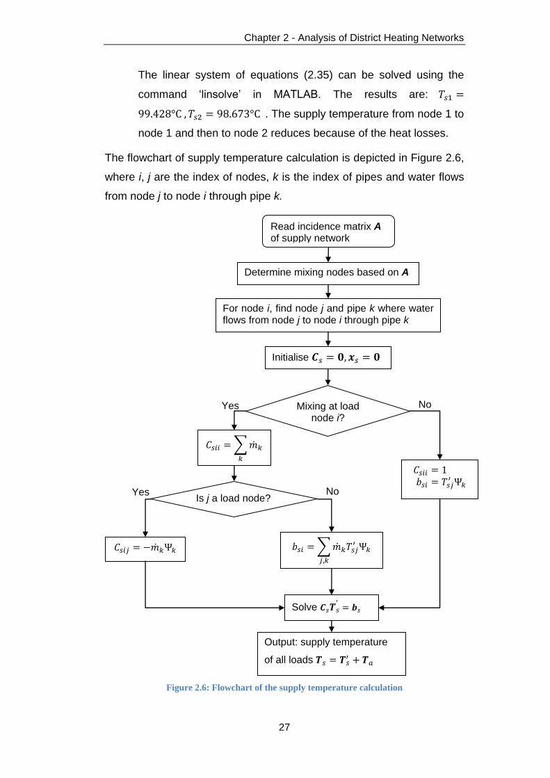
The flowchart of supply temperature calculation is depicted in Figure 2.6,
where i, j are the index of nodes, k is the index of pipes and water flows
from node j to node i through pipe k.
Figure 2.6: Flowchart of the supply temperature calculation
Read incidence matrix A of supply network
Determine mixing nodes based on A
Is j a load node?
Mixing at load node i?
Solve
Output: supply temperature
of all loads
Yes No
Yes No
For node i, find node j and pipe k where water flows from node j to node i through pipe k
Initialise

Chapter 2 - Analysis of District Heating Networks
28
2.4.2 Return Temperature Calculation
The objective is to determine the load and source return temperatures
based on the specified load outlet temperatures. For the return network
shown in Figure 2.5, the incidence matrix is the inverse of the incidence
matrix of the supply network.
(-A) =
The steps of the thermal calculation are similar to that of the supply
network and are performed as follows
1) Determine the mixing nodes based on the matrix (-A). The row 1
in the matrix (-A) has one element ‘1’ plus one incoming flow from
load 1 to the node 1 and row 3 has more than one element ‘1’,
which means the incoming flows mix at the node 1 and 3.
2) For node 1, the return temperature T'r1 is calculated using the
temperature drop equation (2.33) and the temperature mixing
equation (2.34)
(2.36)
3) For node 2, the return temperature T'r2 is equal to the outlet
temperature and calculated as
(2.37)
4) Similarly, the temperature equations (2.36) and (2.37) are
combined to form a linear system of equations
(2.38)
1 2 3
1 -1 1 0
2 0 -1 -1
3 1 0 1
Node N
o.
Pipe No.

Chapter 2 - Analysis of District Heating Networks
29
where is the matrix of coefficients, is the column vector of
variables (the load return temperatures) and is the column
vector of solutions. The general procedure to form matrix and
vector is illustrated using a flowchart in Figure 2.7.
(2.39)
By substituting the specified parameters into equation (2.39)
(2.40)
The linear system of equations (2.40) is solved using the
command ‘linsolve’ in MATLAB. The results are:
5) For source node 3, the return temperature T'r3 is calculated using
the temperature drop equation (2.33) and the temperature mixing
equation (2.34)
(2.41)
The result is: .
The return temperature from node 2 to node 1 reduces because of the
heat losses.
The results of the thermal model are validated together with the hydraulic
model in the next section 2.5.
The flowchart of the return temperature calculation is shown in Figure
2.7.

Chapter 2 - Analysis of District Heating Networks
30
Figure 2.7: Flowchart of the return temperature calculation
Read incidence matrix (-A) of return network
Mixing at load node i?
Solve
Output: return temperature
of all sources
Yes No
Mixing at source node i?
Yes No
Output: return temperature of all loads
For node i, find node j and pipe k where water flows from node j to node i through pipe k
Determine mixing nodes based on (-A)
Initialise

Chapter 2 - Analysis of District Heating Networks
31
2.5 Hydraulic-Thermal Model
2.5.1 Introduction
For a district heating network, the objective of the hydraulic-thermal
model is to determine the mass flow rates within each pipe and the
load supply temperatures and the source return temperatures. It is
assumed that the source supply temperatures and the load return
temperatures are specified; the mass flow rates or the heat power Φ
are specified at all the nodes except the slack node [11, 67, 71, 72]. The
slack node is defined to be rescheduled to supply the heat power
difference between the total system loads plus losses and the sum of
specified heat power at the source nodes.
If the nodal injected mass flow rates is specified, the hydraulic-
thermal model calculations are performed independently [68, 73]. Firstly,
the pipe mass flow rates is calculated by the hydraulic model. Then,
the results of the hydraulic model are substituted into the thermal
model. Finally, the load supply temperatures and the source return
temperatures are calculated by the thermal model.
Alternatively, if the heat power Φ consumed or supplied at each node is
specified, two methods are adopted to perform the calculation of the
hydraulic-thermal model. Conventionally, the calculation is through an
iterative procedure – referred to as the decomposed hydraulic-thermal
calculation – between the individual hydraulic and thermal models [67].
In this thesis, an integrated hydraulic-thermal calculation was proposed,
in which the hydraulic and thermal models were combined in a single
system of equations.
Until now, the Newton-Raphson method has been used in the hydraulic
calculation. The integrated calculation combines the individual hydraulic
and thermal analyses using the Newton-Raphson approach. It takes into
account the coupling between the individual hydraulic and thermal
analyses. For instance, the thermal calculation cannot be performed
without knowing the pipe mass flows. The hydraulic calculation cannot

Chapter 2 - Analysis of District Heating Networks
32
be performed without knowing temperatures under the assumption that
the nodal heat power are specified.
The proposed methods can handle the initial conditions with arbitrary
flow directions. During each iteration of the hydraulic-thermal model, the
network incidence matrix A and the loop incidence matrix B are updated
according to the signs of the pipe mass flow rates. Based on matrix A,
the formulation of the temperature mixing equations in the thermal model
is updated at each iteration.
2.5.2 Decomposed Hydraulic-Thermal Calculation
The structure of the decomposed hydraulic-thermal calculation with
specified nodal heat power is shown in Figure 2.8. The iterative
procedure between the individual hydraulic and thermal models is as
follows
· The calculated nodal mass flow rates are substituted into the
hydraulic model to update the pipe mass flow rates . For the first
iteration, is initialised.
· The load supply temperatures and the source return
temperatures are updated using the thermal model.
· The calculated temperatures are fed back into the heat power
equation (2.31) to update the nodal injected mass flow rates .
Figure 2.8: Structure of the decomposed hydraulic-thermal calculation with specified
nodal heat power
Decomposed Hydraulic-Thermal model
Network
data
Hydraulic
model
Thermal
model Output
Heat power
equation
m ·
Ts,load
Tr,source
Specified Φ,
Ts,source
To,load
Network
topology
Length,
diameter,
roughness
of each pipe
Ambient Ta
Ts,source
To,load
Nodal heat
power Φ
Ts,load
Tr,load
Tr,source
Heat losses
m ·
mq ·

Chapter 2 - Analysis of District Heating Networks
33
The flowchart of the decomposed hydraulic-thermal calculation with
specified nodal heat power is shown in Figure 2.9. Denoting
,
, where i is the iteration time. The
initialised load supply temperatures and the initialised source
return temperatures are substituted into the heat power equation
(2.31) to calculate the nodal flows .
Max(ΔTs,load, ΔTr) <ε?
Calculate Ts,load, Tr
Input: Φ
To,load
Ts,source
Initialise Ts,load, Tr (Tr,load, Tr,source)
Form hydraulic
equations
Linear equations
Radial
network
Looped
network
Calculate m
Nonlinear equations
Form thermal
equations
Apply temperature drop
and mixing equations
Determine mixing nodes
Apply temperature
drop equations
Non-mix Mix
Hydraulic
model
Yes
.
No
Calculate ΔTs,load, ΔTr
Thermal
model
Calculate nodal flows mq
by Heat power equations
.
Outputs:
m, Ts,load, Tr,
slack node Φ
.
Figure 2.9: Flowchart of the decomposed hydraulic-thermal calculation with specified
nodal power

Chapter 2 - Analysis of District Heating Networks
34
A simple district heating network with a loop shown in Figure 2.10 is
used to illustrate the decomposed hydraulic-thermal calculation. The
objective is to determine the pipe mass flow rates and the
load supply temperatures Ts1,load, Ts2,load and the source return
temperature Tr1,source. The specified variables are [67]: Φ1,load = Φ2,load =
0.3MW. Ts1,source = 100°C, To1,load = To2,load = 50°C. The ambient
temperature Ta = 10°C. The parameters of each pipe are [67]: L1 = L2 =
400m, L3 = 600m, D = 0.15m, ε = 1.25×10⁻³m, λ = 0.2W/mK. Cp =
4182J/(kg·K)) = 4.182 × 10⁻³MJ/(kg·K)).
Load2
3
1 2
Source1
Load1
Load2
To1,load To2,load
Ts1,source
Φ1,load Φ2,load
Tr1,source
1 23
Figure 2.10: A district heating network with a loop
The continuity of flow is applied to all nodes in a network, but one is
redundant because of it being linearly dependent on others and is
chosen arbitrarily for exclusion. Thus, the last row of the network
incidence matrix A that relates to the slack node is redundant and is
chosen for exclusion.
For the supply network shown in Figure 2.10,
A =
B =
(2.35)
Each element of the matrix A describes
+1, if the flow in a pipe comes into a node;
-1, if the flow in a pipe leaves a node;
0, if no connection from a pipe to a node.
1 2 3
1 1 1 -1
Pipe No. 1 2 3
1 1 -1 0
2 0 1 1
Node N
o.
Pipe No.
Loop N
o.

Chapter 2 - Analysis of District Heating Networks
35
Each element of the matrix B describes
+1, if the flow in a pipe has the same direction as the definition;
-1, if the flow in a pipe has the opposite direction as the definition;
0, if pipe is not part of the loop.
Following equations (2.25) and (2.26), the vector of mismatches ΔF and
the Jacobian matrix J are
(2.36)
(2.37)
The steps used to solve the decomposed calculation of the district
heating network in Figure 2.10 are as follows
Step 1) Assume initial condition as,
,
.
Step 2) Calculate the nodal flows using the heat power
equation (2.31),
. For the first iteration,
kg/s.
Step 3) Update using the hydraulic model.
For the first iteration,
,
,
,
.

Chapter 2 - Analysis of District Heating Networks
36
Step 4) Update using the thermal model. For the
first iteration,
,
.
Step 5) This procedure is repeated from step 2) until the maximal
and become less than ε.
After 4 iterations with the tolerance ε = 10-3, the converged results are
. Ts1,load = 98.958, Ts2,load = 97.140.
Tr1,load = 49.558, Tr2,load = 50, Tr1,source = 49.125.
To validate the results, the network in Figure 2.10 is analysed using
commercial software SINCAL [67]. The results are the same with
SINCAL at 10-3 precision. A screenshot of the result Ts1,load = 98.958 in
SINCAL is shown in Figure 2.11.
Figure 2.11: Result of the supply temperature at the load 1 from SINCAL
2.5.3 Integrated Hydraulic-Thermal Calculation
The integrated hydraulic-thermal calculation combines the individual
hydraulic and thermal analyses in a single system of equations under the
assumption of specified nodal heat power. The single system of
equations was solved by the Newton-Raphson method with an integrated
Jacobian matrix.

Chapter 2 - Analysis of District Heating Networks
37
The system of equations for the integrated hydraulic-thermal calculation
is derived from the individual hydraulic and thermal models, which is
illustrated in Figure 2.12. The individual hydraulic and thermal models
are linked through the pipe mass flow rates . To form the integrated
hydraulic-thermal model, a heat power equation describing the relation
between the nodal heat power and the pipe mass flow rates is
expressed as equation (2.42). It is obtained by substituting the nodal
flows in the continuity equation (2.4) into the heat power equation
(2.31) to eliminate the intermediate variables .
(2.42)
where Φ is the vector of heat power (MWth) consumed or supplied at
each node; is the specific heat of water, = 4.182 × 10⁻³ MJ/(kg·K));
A is the network incidence matrix, and the last row of A that relates to
the slack node is redundant and is chosen for exclusion; is the mass
flow rates (kg/s) within each pipe; Ts is the supply temperatures (°C); To
is the outlet temperatures (°C).
Figure 2.12: Derivation of the system of equations for the integrated hydraulic-thermal
calculation
Substitute q
Hydraulic model
Thermal model
Continuity equations f1( ) = q
Loop pressure equations f2( ) = 0
Heat power equations f3( q, Ts) = Φ
Supply temperature equations f4( , Ts)= 0
Integrated Hydraulic-Thermal model
Heat power equations f3( , Ts) - Φ = 0
Loop pressure equations f2( ) = 0
Supply temperature equations f4( , Ts) = 0
Return temperature equations f5( , Tr) = 0
Return temperature equations f5( , Tr) = 0
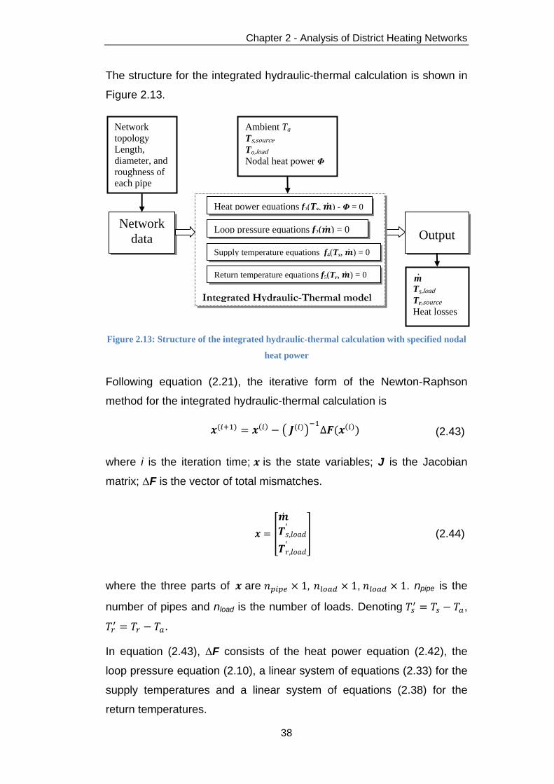
Chapter 2 - Analysis of District Heating Networks
38
The structure for the integrated hydraulic-thermal calculation is shown in
Figure 2.13.
Figure 2.13: Structure of the integrated hydraulic-thermal calculation with specified nodal
heat power
Following equation (2.21), the iterative form of the Newton-Raphson
method for the integrated hydraulic-thermal calculation is
(2.43)
where i is the iteration time; is the state variables; J is the Jacobian
matrix; ΔF is the vector of total mismatches.
(2.44)
where the three parts of are , , . npipe is the
number of pipes and nload is the number of loads. Denoting ,
.
In equation (2.43), ΔF consists of the heat power equation (2.42), the
loop pressure equation (2.10), a linear system of equations (2.33) for the
supply temperatures and a linear system of equations (2.38) for the
return temperatures.
Network
data Output
Network
topology
Length,
diameter, and
roughness of
each pipe
Ambient Ta
Ts,source
To,load
Nodal heat power Φ
Ts,load
Tr,source
Heat losses
m ·
Integrated Hydraulic-Thermal model
Heat power equations f3(Ts, ) - Φ = 0
Loop pressure equations f2( ) = 0
Supply temperature equations f4(Ts, ) = 0
Return temperature equations f5(Tr, ) = 0

Chapter 2 - Analysis of District Heating Networks
39
(2.45)
where is the specified nodal heat power. The four parts of ΔF are
, , and . nnode is the number of
nodes, and nload is the number of loads, and nloop is the number of loops.
Hence, following equations (2.44) and (2.45), the integrated Jacobian
matrix J comprises (3 × 3 block) matrices. It is divided by the mass flow
rates, the supply temperatures and the return temperatures.
(2.46)
where the block matrices in grey background are nonzero and others are
zero. The nonzero elements of the off-diagonal submatrices and in
the Jacobian matrix are the derivatives of the mixture temperatures
mismatches to the mass flow rates . Thus, they are usually very small
relative to the elements of the diagonal submatrices , and . This
is because the small variation of mass flow rates has very small variation
to the difference of the mixture temperature. For simplicity, the
submatrices and in the Jacobian matrix are put to zero [85].
Following equations (2.45) and (2.46), is similar to the Jacobian
matrix in the hydraulic model as shown in equation (2.26).
(2.47)

Chapter 2 - Analysis of District Heating Networks
40
where the upper part of is ; the lower part of is
.
Following equations (2.45) and (2.46), is expressed as
(2.48)
where is . Diag [E] represents a matrix with the elements
E on the diagonal.
Following equations (2.45) and (2.46), and are equal to the
coefficients matrix for supply and return networks in the thermal model.
(2.49)
where is and is .
To illustrate the integrated hydraulic-thermal calculation, the model
equations are applied to the district heating network in Figure 2.10. Thus,
npipe = 3, nnode = 3, nload = 2 and nloop = 1.
Following equation (2.44), the state variables x for the network shown in
Figure 2.10 is given by
(2.50)
Following equation (2.45), the vector of total mismatches ΔF for the
network in Figure 2.10 consists of the heat power equation (2.45), the
loop pressure equation (2.28), a linear system of equations for the supply
temperatures (2.34) and a linear system of equations for the return
temperatures (2.39). ΔF for the network shown in Figure 2.10 is given by

Chapter 2 - Analysis of District Heating Networks
41
(2.51)
where the last row of A that relates to the slack node is redundant and is
chosen for exclusion.
.
Hence, following equation (2.46), the Jacobian matrix is expressed as
(2.52)
Following equation (2.47), is expressed as
(2.53)
Following equation (2.48), is expressed as
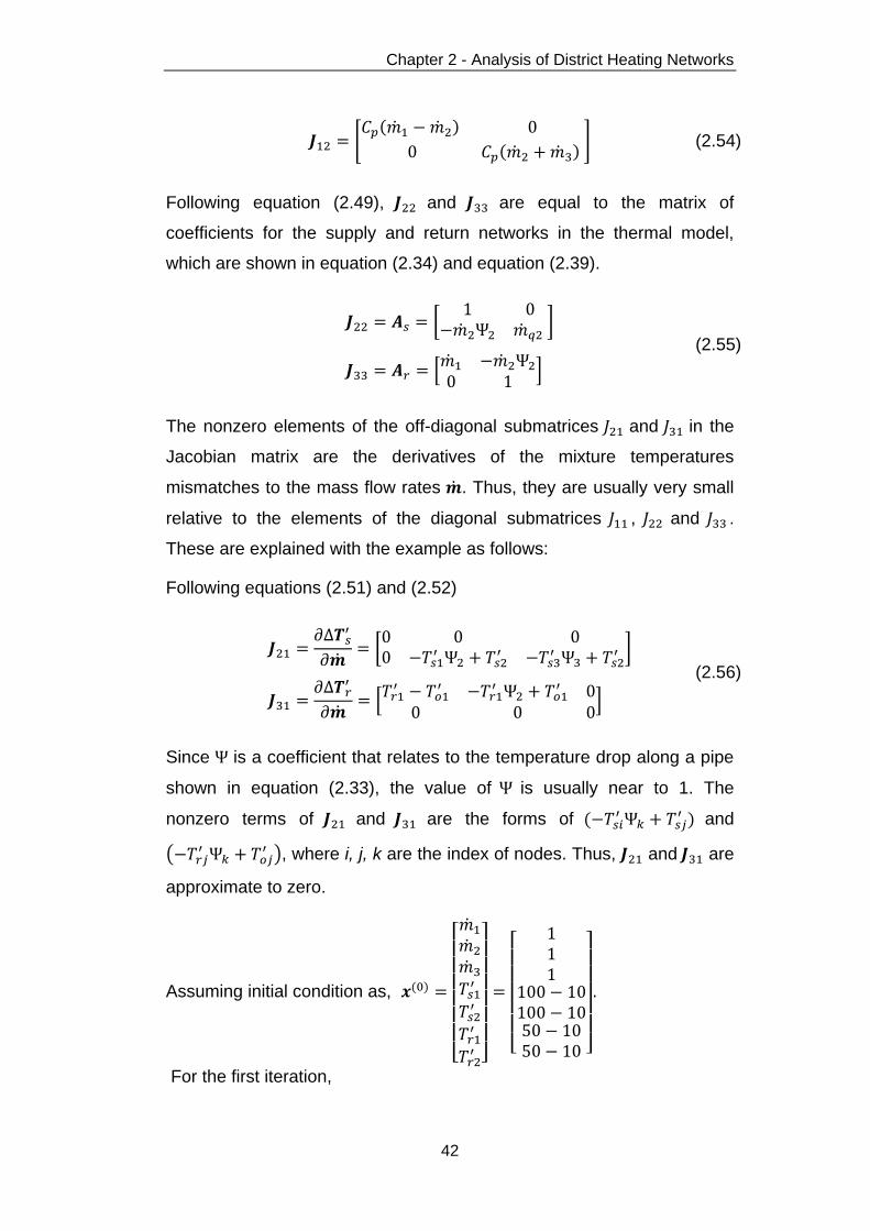
Chapter 2 - Analysis of District Heating Networks
42
(2.54)
Following equation (2.49), and are equal to the matrix of
coefficients for the supply and return networks in the thermal model,
which are shown in equation (2.34) and equation (2.39).
(2.55)
The nonzero elements of the off-diagonal submatrices and in the
Jacobian matrix are the derivatives of the mixture temperatures
mismatches to the mass flow rates . Thus, they are usually very small
relative to the elements of the diagonal submatrices , and .
These are explained with the example as follows:
Following equations (2.51) and (2.52)
(2.56)
Since is a coefficient that relates to the temperature drop along a pipe
shown in equation (2.33), the value of is usually near to 1. The
nonzero terms of and are the forms of
and
, where i, j, k are the index of nodes. Thus, and are
approximate to zero.
Assuming initial condition as,
.
For the first iteration,

Chapter 2 - Analysis of District Heating Networks
43
,
Following equation (2.43),
.
The procedure is repeated until the maximum element in the mismatches
becomes less than the tolerance ε = 10-3. After 5 iterations, the
converged results are shown in Table 2.3. The results of the
decomposed and integrated calculations are very close. The small
differences are due to the simplification of the integrated Jacobian matrix
in the integrated hydraulic-thermal calculation and the different stopping
criteria of two calculations.
Table 2.3: Results of the decomposed and integrated hydraulic-thermal calculations
Decomposed
hydraulic and thermal
calculation
.
Ts1,load = 98.9576, Ts2,load = 97.1401.
Tr1,load = 49.5583, Tr2,load = 50, Tr1,source = 49.1251.
Integrated
hydraulic-thermal
calculation
.
Ts1,load = 98.9575, Ts2,load = 97.1400.
Tr1,load = 49.5583, Tr2,load = 50, Tr1,source = 49.1251.
2.6 Summary
Hydraulic-thermal model was developed to investigate the performance
of a district heating network. The objective of the hydraulic-thermal
model was to determine the mass flow rates within each pipe and the

Chapter 2 - Analysis of District Heating Networks
44
load supply temperatures and the source return temperatures. It was
assumed that the supply temperatures of the source and the return
temperatures of the load are specified; the injected mass flow rates or
the heat power supplied or consumed at all the nodes except one are
specified.
The individual hydraulic and thermal models in district heating networks
were modelled. In the hydraulic model, the network description was
based on a graph-theoretical method and the Newton-Raphson method
was used to solve the hydraulic equations for looped networks. In the
thermal model, the mixture temperatures at nodes were considered and
a matrix formulation of the thermal model was implemented.
Conventionally, the decomposed hydraulic-thermal calculation was
through an iterative procedure between the individual hydraulic and
thermal models. In this thesis, an integrated hydraulic-thermal calculation
was developed, in which the hydraulic and thermal models were
combined in a single system of equations solved by the Newton-
Raphson method. The results of two calculations were very close and
the results were validated using SINCAL with the same values at 10-3
precision.

Chapter 3 - Combined Analysis of Electricity
and Heat Networks
3.1 Introduction
3.1.1 Combined Electricity and District Heating Networks
A schematic for combined electricity and district heating networks is
shown in Figure 3.1. The electricity and heat networks are linked through
the coupling components (e.g., CHP units, heat pumps, electric boilers
and circulation pumps), which are represented as the Sources in Figure
3.1. These coupling components allow flows of energy between the two
networks. The CHP units generate electricity and heat simultaneously;
heat pumps and electric boilers convert electricity to heat; circulation
pumps consume electricity to circulate water in the district heating
network. The coupling components are generalised as an electrical and
heat interface with adjustable heat-to-power ratio. These coupling
components increase the flexibility of the electricity and heat supply
systems for facilitating the integration of intermittent renewable energy.
An illustration of the energy flow of a CHP and heat pump composite
supply system is shown in Figure 3.2.
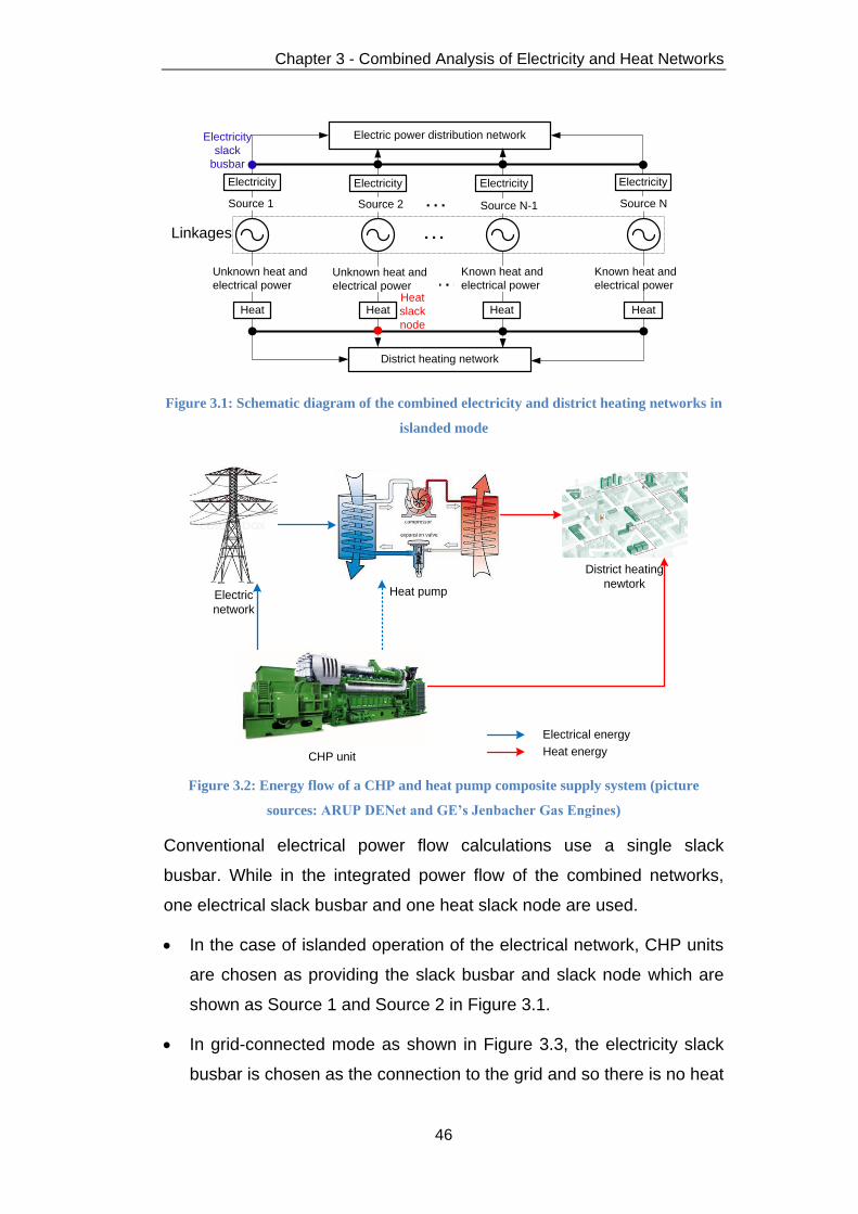
Chapter 3 - Combined Analysis of Electricity and Heat Networks
46
Electricity
Heat
Electricity
Unknown heat and
electrical power
…
District heating network
Electric power distribution networkElectricity
slack
busbar
HeatHeat
slack
node
Electricity Electricity
Heat Heat
Linkages
Source 2 Source N-1Source 1 …
…
Source N
Unknown heat and
electrical power
Known heat and
electrical power
Known heat and
electrical power
Figure 3.1: Schematic diagram of the combined electricity and district heating networks in
islanded mode
Heat pumpElectric
network
CHP unit
Electrical energy
Heat energy
District heating
newtork
Figure 3.2: Energy flow of a CHP and heat pump composite supply system (picture
sources: ARUP DENet and GE’s Jenbacher Gas Engines)
Conventional electrical power flow calculations use a single slack
busbar. While in the integrated power flow of the combined networks,
one electrical slack busbar and one heat slack node are used.
· In the case of islanded operation of the electrical network, CHP units
are chosen as providing the slack busbar and slack node which are
shown as Source 1 and Source 2 in Figure 3.1.
· In grid-connected mode as shown in Figure 3.3, the electricity slack
busbar is chosen as the connection to the grid and so there is no heat

Chapter 3 - Combined Analysis of Electricity and Heat Networks
47
generated at the electricity slack busbar. Therefore, the grid-
connected mode can be considered as a simplified special case of
islanded operation.
Other than the CHP unit providing the electricity slack busbar, CHP units
with adjustable real power output and voltage magnitude are classified
as PV busbars; the other CHP units such as micro-CHP are classified as
PQ busbars.
Heat
Electricity
Unknown electrical power
Know heat power
…
District heating network
Electric power distribution networkElectricity
slack
busbar
HeatHeat
slack
node
Electricity Electricity
Heat Heat
Source 2 Source N-1…
…
Source N
Unknown heat and
electrical power
Known heat and
electrical power
Known heat and
electrical power
Grid-connection
point
Electricity
Figure 3.3: Schematic diagram of the combined electricity and district heating networks in
grid-connected mode
The CHP units and other coupling components allow flows of energy
between the two networks. In islanded mode, the heat power generated
by Source 2 (at the electricity slack busbar) is determined by the
electrical power generated from this unit. Similarly, the electrical power
generated from Source 1 (at the heat slack node) is a function of the
heat network. Neither the heat network nor the electricity network can be
calculated without taking into account the other network. It is assumed
that the heat and electrical power generated by the CHP units is fully
utilised without heat dumping.
Two calculation techniques were developed to calculate the operating
points of the electricity and heat networks as follows. The schematics of
the two calculation techniques are shown in Figure 3.4, where x(i) is the
vector of unknown state variables at the ith iteration.

Chapter 3 - Combined Analysis of Electricity and Heat Networks
48
· In the decomposed electrical-hydraulic-thermal calculation, the
independent hydraulic equations and thermal equations and electrical
power flow equations were calculated sequentially and linked through
the coupling components. This is based on the decomposed
hydraulic-thermal calculation of district heating networks in Chapter 2.
This sequential procedure is iterated at each time step until the
solution converges to an acceptable tolerance (Figure 3.4a.i). Grid-
connected operation is a special case of the sequential method
(Figure 3.4a.ii). Here only one calculation is taken between the
independent hydraulic calculation and thermal calculation and
electrical power flow calculation.
· In the integrated electrical-hydraulic-thermal calculation, the electrical
power flow equations, the hydraulic equations, and the thermal
equations were combined and solved simultaneously as an integrated
whole (Figure 3.4b). This is based on the integrated hydraulic-thermal
calculation of district heating networks in Chapter 2.

Chapter 3 - Combined Analysis of Electricity and Heat Networks
49
Figure 3.4: Schematics of the decomposed electrical-hydraulic-thermal calculation (a.i) in
grid-connected mode and (a.ii) islanded mode and (b) the integrated electrical-hydraulic-
thermal calculation
The structure of the integrated electrical-hydraulic-thermal calculation is
shown in Figure 3.5. The hydraulic and thermal model equations are
linked through the mass flow rates. The electrical power flow equations
and hydraulic-thermal model equations are linked through the coupling
components. The equations of the integrated electrical-hydraulic-thermal
model are derived from the equations of the electrical power flow, the
hydraulic model, the thermal model and the coupling components model.
Thermal Equations
Electric Power Flow Equations
Hydraulic Equations
x(i+1) x
(i)
Hydraulic Equations
Thermal Equations
Electric Power Flow Equations
x(i)
x(i+1)
(a.ii)
Thermal Equations
Electric Power Flow Equations
Hydraulic Equations
(b)
(a.i)
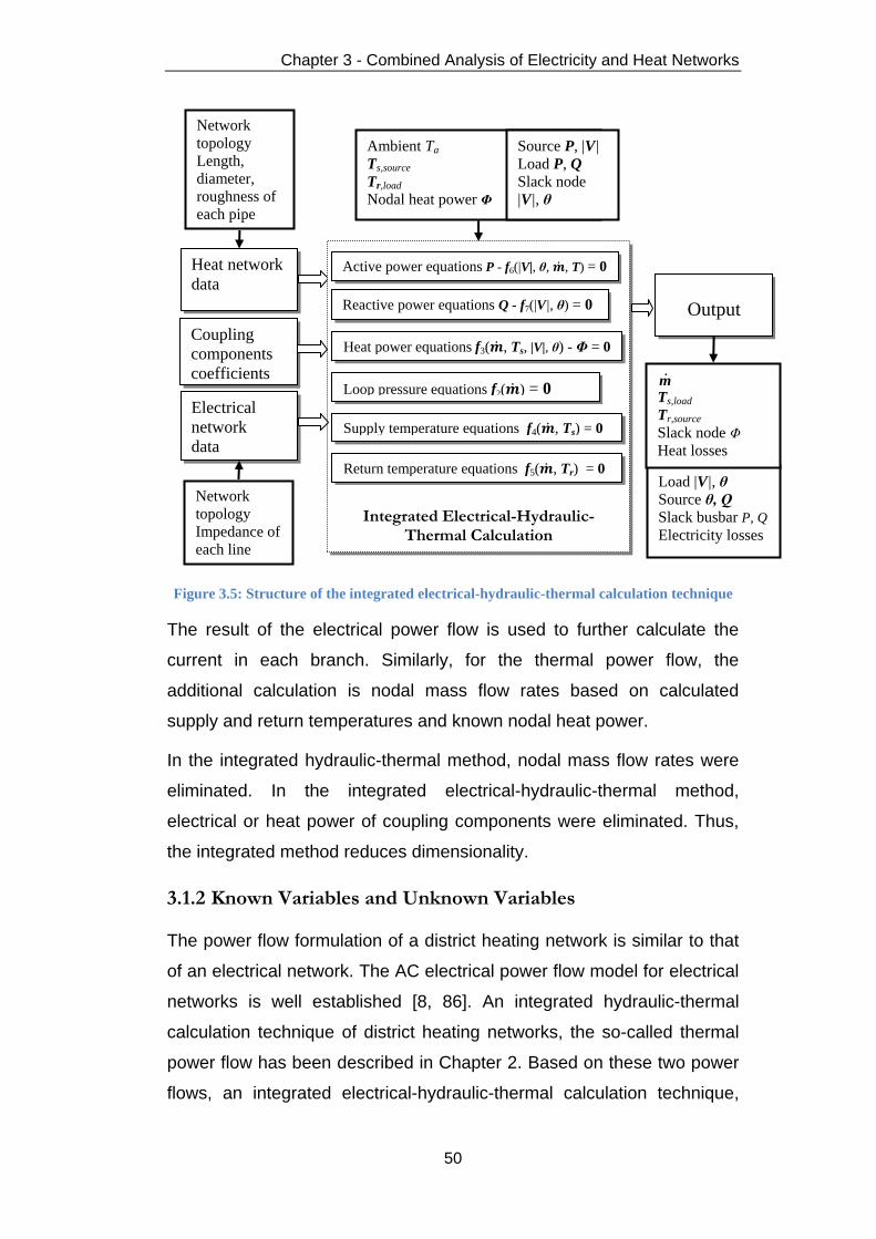
Chapter 3 - Combined Analysis of Electricity and Heat Networks
50
Figure 3.5: Structure of the integrated electrical-hydraulic-thermal calculation technique
The result of the electrical power flow is used to further calculate the
current in each branch. Similarly, for the thermal power flow, the
additional calculation is nodal mass flow rates based on calculated
supply and return temperatures and known nodal heat power.
In the integrated hydraulic-thermal method, nodal mass flow rates were
eliminated. In the integrated electrical-hydraulic-thermal method,
electrical or heat power of coupling components were eliminated. Thus,
the integrated method reduces dimensionality.
3.1.2 Known Variables and Unknown Variables
The power flow formulation of a district heating network is similar to that
of an electrical network. The AC electrical power flow model for electrical
networks is well established [8, 86]. An integrated hydraulic-thermal
calculation technique of district heating networks, the so-called thermal
power flow has been described in Chapter 2. Based on these two power
flows, an integrated electrical-hydraulic-thermal calculation technique,
Load |V|, θ
Source θ, Q
Slack busbar P, Q
Electricity losses
Heat network
data
Output
Network
topology
Length,
diameter,
roughness of
each pipe
Ts,load
Tr,source
Slack node Φ
Heat losses
Ambient Ta
Ts,source
Tr,load
Nodal heat power Φ
m ·
Integrated Electrical-Hydraulic-Thermal Calculation
Active power equations P - f6(|V|, θ, , T) = 0
Reactive power equations Q - f7(|V|, θ) = 0
Electrical
network
data
Network
topology
Impedance of
each line
Source P, |V|
Load P, Q
Slack node
|V|, θ
Coupling
components
coefficients
Heat power equations f3( , Ts, |V|, θ) - Φ = 0
Loop pressure equations f2( ) = 0
Supply temperature equations f4( , Ts) = 0
Return temperature equations f5( , Tr) = 0
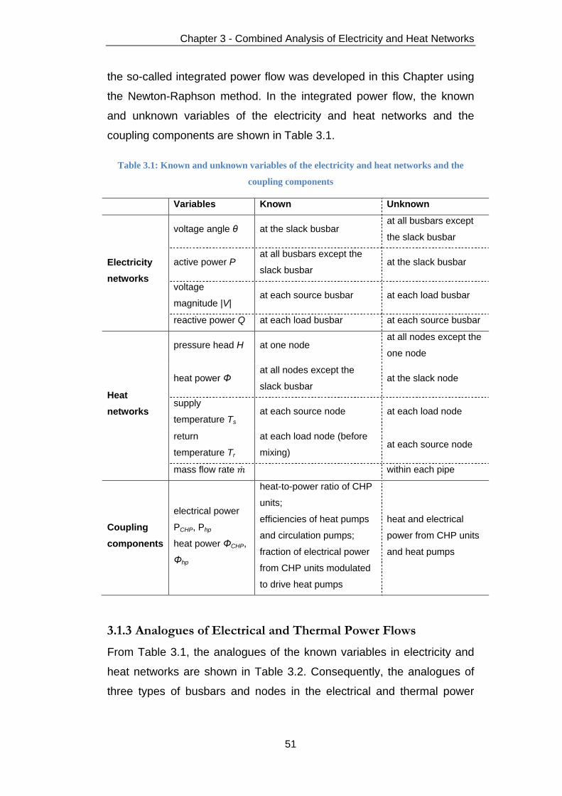
Chapter 3 - Combined Analysis of Electricity and Heat Networks
51
the so-called integrated power flow was developed in this Chapter using
the Newton-Raphson method. In the integrated power flow, the known
and unknown variables of the electricity and heat networks and the
coupling components are shown in Table 3.1.
Table 3.1: Known and unknown variables of the electricity and heat networks and the
coupling components
Variables Known Unknown
Electricity
networks
voltage angle θ at the slack busbar at all busbars except
the slack busbar
active power P at all busbars except the
slack busbar at the slack busbar
voltage
magnitude |V| at each source busbar at each load busbar
reactive power Q at each load busbar at each source busbar
Heat
networks
pressure head H at one node at all nodes except the
one node
heat power Φ at all nodes except the
slack busbar at the slack node
supply
temperature Ts at each source node at each load node
return
temperature Tr
at each load node (before
mixing) at each source node
mass flow rate within each pipe
Coupling
components
electrical power
PCHP, Php
heat power ΦCHP,
Φhp
heat-to-power ratio of CHP
units;
efficiencies of heat pumps
and circulation pumps;
fraction of electrical power
from CHP units modulated
to drive heat pumps
heat and electrical
power from CHP units
and heat pumps
3.1.3 Analogues of Electrical and Thermal Power Flows
From Table 3.1, the analogues of the known variables in electricity and
heat networks are shown in Table 3.2. Consequently, the analogues of
three types of busbars and nodes in the electrical and thermal power

Chapter 3 - Combined Analysis of Electricity and Heat Networks
52
flows are shown in Table 3.3. Each type of busbar and node is classified
according to two known quantities.
Table 3.2: Analogues of the known variables in electricity and heat networks
Busbar (Node) Electricity Networks District Heating Networks
slack busbar (node) voltage angle θ pressure head H
all busbars except
the slack busbar (node) active power P heat power Φ
source busbar (node) voltage magnitude |V| supply temperature Ts
load busbar (node) reactive power Q return temperature Tr
Table 3.3: Analogues of busbar and node types in electrical and thermal power flows
Electrical power flow P Q busbar P V busbar V θ busbar
Thermal power flow Φ Tr node Φ Ts node Ts H node
3.2 Coupling Components Model
The electricity and heat networks are linked through the coupling
components (CHP units, heat pumps, electric boilers and circulation
pumps). From the modelling point of view, heat pumps or electric boilers
are equivalent to CHP units with negative electrical power output;
electrical power generators are equivalent to CHP units with zero heat
output. These components are generalised as an electrical and heat
interface with adjustable heat-to-power ratio. The heat and electrical
power outputs of the interface are described by their equivalent heat-to-
power ratios as was introduced by Mancarella [62].
3.2.1 CHP Units
Three types of CHP units are discussed: gas turbines, internal
combustion reciprocating engines and steam turbine CHP units.

Chapter 3 - Combined Analysis of Electricity and Heat Networks
53
For CHP units using gas turbines or internal combustion reciprocating
engines, then the relation between heat and electrical power generation
is simplified as equation (3.1) and the schematic is shown in Figure 3.7
(a). It can be seen that the heat-to-power ratio is constant [19, 87].
(3.1)
where PCHP (MWe) is the electrical power output and ΦCHP (MWth) is the
useful heat output of CHP units. The outputs are varied by the fuel input
rate. cm is the heat-to-power ratio [88].
Steam turbine CHP units may be divided into: condensing units and
back-pressure units [89, 90]. In the condensing units, no heat is used for
industrial processes or district heating purposes. In the back-pressure
units, the remaining heat after the turbine can be used for heating
purposes with the temperature and pressure of the exhaust steam being
higher than that of condensing units [91]. In an extraction steam turbine
as shown in Figure 3.6, some steam is extracted at an intermediate
pressure for the supply of useful heat [26]. Extraction units may vary
from full condensing to full extraction mode by changing the extraction
ratio and thus possess the ability to adjust the ratio between useful heat
extracted and electrical power generation [19, 26, 91, 92]. A fraction of
extraction of 1 denotes full extraction mode and 0 denotes full
condensing mode.
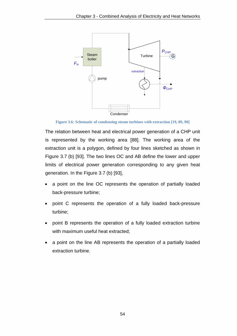
Chapter 3 - Combined Analysis of Electricity and Heat Networks
54
GSteam
boiler
Condenser
pump
ΦCHP
PCHP
Fin
extraction
Turbine
Figure 3.6: Schematic of condensing steam turbines with extraction [19, 89, 90]
The relation between heat and electrical power generation of a CHP unit
is represented by the working area [88]. The working area of the
extraction unit is a polygon, defined by four lines sketched as shown in
Figure 3.7 (b) [93]. The two lines OC and AB define the lower and upper
limits of electrical power generation corresponding to any given heat
generation. In the Figure 3.7 (b) [93],
· a point on the line OC represents the operation of partially loaded
back-pressure turbine;
· point C represents the operation of a fully loaded back-pressure
turbine;
· point B represents the operation of a fully loaded extraction turbine
with maximum useful heat extracted;
· a point on the line AB represents the operation of a partially loaded
extraction turbine.

Chapter 3 - Combined Analysis of Electricity and Heat Networks
55
Ele
ctr
ica
l p
ow
er
(PC
HP)
Useful heat power(ΦCHP)
Ele
ctr
ica
l p
ow
er
(PC
HP)
Useful heat power(ΦCHP)
C
B
A
O
-1/Z
ΔP
ΔΦ
Pcon
(a) (b)
Figure 3.7: The relation between heat and electrical power generation of CHP units: (a)
gas turbines or internal combustion engines and (b) extraction steam turbines [93]
For the steady state analysis in this thesis, the relation between heat and
electrical power generation of the extraction unit is chosen as the line AB
shown in Figure 3.7 (b). For a given fuel consumption, the electrical
power efficiency will decline as steam extraction increases [94]. The
relation is described using equation (3.2)
(3.2)
where Z is the ratio that describes the trade-off between heat supplied to
site and electrical power (Z = 3.9 ~ 8.1) [94]. is the increased heat
recovery and is the reduced electrical power output. PCHP (MWe) is
the electrical power output and ΦCHP (MWth) is the useful heat output of
extraction units. They are shown in the Figure 3.6. Pcon (MWe) is the
electrical power generation of the extraction unit in full condensing mode,
shown in Figure 3.7 (b).
(3.3)
where is the electrical efficiency of the extraction unit in full
condensing mode; Fin (MW) is the fuel input rate which is held constant
in this thesis.

Chapter 3 - Combined Analysis of Electricity and Heat Networks
56
Following equation (3.2), (-1/Z) represents the slope of the line AB and
Pcon represents the intercept value in Figure 3.7 (b).
Extraction steam turbines allow a wide range of heat-to-power ratios
which are varied by the extraction ratio. In islanded mode, a gas turbine
and an extraction turbine CHP units are chosen as providing the slack
busbar and slack node. Since two CHP units with contrary properties that
slope upwards and downwards are more likely to be able to meet both
electricity and heat demands. It is assumed that the heat and electrical
power generated by the CHP units is fully utilised without heat dumping.
3.2.2 Heat Pumps
Heat pumps use a small quantity of electricity to leverage heat from the
surroundings to higher temperatures, using a compressor just like a
refrigerator [22, 32]. Heat pumps are more energy efficient than gas
boilers, typically producing three units of heat for every unit of electricity
[22]. On the other hand, heat pumps have higher investment costs and
also use more expensive fuel [60]. There are two types of heat pumps:
air source and ground source heat pumps. The efficiency of a heat pump
is modelled as
(3.4)
where the coefficient of performance (COP) is the ratio of heat power
supplied (MWth) to electrical power consumed (MWe). The COP
of a heat pump varies according to the magnitude of the temperature
difference between the heat source and the heat load [33].
3.2.3 Electric Boilers
Electric boilers consume electricity to generate heat. The efficiency of an
electric boiler is calculated as
(3.5)

Chapter 3 - Combined Analysis of Electricity and Heat Networks
57
where ηb represents the efficiency of an electric boiler; Pb (MWe) and Φb
(MWth) are the electrical power consumed and the heat power supplied.
3.2.4 Circulation Pumps
A circulation pump is located at the heat plant to create and maintain
pressure difference between supply and return lines. The pressure
difference of a pump at a supply must be high enough to ensure that the
node farthest away from the pump still has a sufficient minimum pressure
difference to allow the water to pass from the supply line through the
heat exchanger into the return line [13, 19, 95]. The consumed electrical
power by a circulation pump is calculated as
(3.6)
where is the electrical power consumed (MWe) by a circulation pump;
is the mass flow rate (kg/s) through the pump; ηp is the efficiency of
the pump; Hp is the pump head (m) of the network. The pump head is
selected to overcome the flow resistance in the supply and return pipes
and also the head differential in the customer installation that is
hydraulically the furthest from the delivery point [14]. The pump head is
calculated as [11, 14]
(3.7)
where Hc is the minimum allowable head differential (m); is the head
losses (m) within a pipe; is a set which includes all the pipes in the
critical route with the largest pressure drop in the network.
3.2.5 Combined Coupling Components
A CHP and heat pump composite supply system is modelled. Heat
pumps are connected to the CHP units in cascade and fed by
cogenerated electrical power, shown in Figure 3.8. It is assumed that the
heat pumps can be operated at partial load. The modelling of the

Chapter 3 - Combined Analysis of Electricity and Heat Networks
58
composite supply system is similar to that of CHP units. The heat and
electrical power outputs of the composite supply system are described
by an equivalent heat-to-power ratio as was introduced by Mancarella
[62].
Figure 3.8: A CHP and heat pump composite supply system
For a CHP and heat pump composite supply system shown in Figure
3.8, the heat and electrical power outputs of the composite supply
system are
(3.8)
where (MWe) is the electrical power output of the composite
supply system and (MWth) is the useful heat output; α is the
percentage of a fraction of electrical power from the CHP units
modulated to drive the heat pumps.
Hence, the equivalent heat-to-power ratio is calculated as
(3.9)
Equations (3.8) and (3.9) illustrate that feeding the heat pumps with
cogenerated electrical power brings about a net increase in heat
production at the cost of net electrical power production [62].
For different types of CHP units, the relation between the heat and
electrical power generation of the composite supply system is described
as follows
CHP units
Heat pumps α
1-α

Chapter 3 - Combined Analysis of Electricity and Heat Networks
59
· For CHP units using gas turbines or internal combustion reciprocating
engines, substituting from equation (3.1) into equation (3.9),
yields
(3.10)
· For CHP units using extraction steam turbines, substituting from
equation (3.2) into equation (3.8), yields
(3.11)
Thus, rearranging the variable to be on one side of equation
(3.11), yields
(3.12)
Thus, substituting equation (3.12) into equation (3.8), yields
(3.13)
Furthermore, if the circulation pump at a CHP unit is taken into account,
in equation (3.8) is written as
(3.14)
where is the consumed electrical power (MWe) by a circulation pump
and is calculated using equation (3.6).
3.3 Electrical Power Flow Analysis
Since the thermal power flow has been described in Chapter 2, this
section focuses on the electrical power flow. The AC electrical power
flow model for electrical networks is well established [8, 86]. Given a
power system described by an admittance matrix, and given a subset of

Chapter 3 - Combined Analysis of Electricity and Heat Networks
60
voltage magnitudes, voltage angles and real and reactive power
injections, the electrical power flow determines the other voltage
magnitudes and angles and real and reactive power injections.
The voltage V at busbar i is given in polar coordinates by
(3.15)
where j is the imaginary unit.
The current injected into the network at busbar i is given by
(3.16)
where N is the number of busbars in the electricity network; Y is the
admittance matrix that relates current injections at a busbar to the busbar
voltages. Current injections may be either positive (into the busbar) or
negative (out of the busbar).
Thus, the calculated complex power injected at busbar i is
(3.17)
Equation (3.17) constitutes the polar form of the electrical power flow
equations.
The specified complex power being injected into the network at busbar i
is the complex power difference between the source and the load.
(3.18)
Following equations (3.17) and (3.18), the electrical complex power
mismatches ∆Si injected at busbar i are denoted as the specified value
minus the calculated value Si.
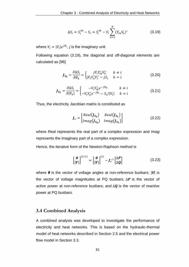
Chapter 3 - Combined Analysis of Electricity and Heat Networks
61
(3.19)
where , j is the imaginary unit.
Following equation (3.19), the diagonal and off-diagonal elements are
calculated as [96]
(3.20)
(3.21)
Thus, the electricity Jacobian matrix is constituted as
(3.22)
where Real represents the real part of a complex expression and Imag
represents the imaginary part of a complex expression.
Hence, the iterative form of the Newton-Raphson method is
(3.23)
where θ is the vector of voltage angles at non-reference busbars; |V| is
the vector of voltage magnitudes at PQ busbars; is the vector of
active power at non-reference busbars; and is the vector of reactive
power at PQ busbars.
3.4 Combined Analysis
A combined analysis was developed to investigate the performance of
electricity and heat networks. This is based on the hydraulic-thermal
model of heat networks described in Section 2.5 and the electrical power
flow model in Section 3.3.
Chapter 3 - Combined Analysis of Electricity and Heat Networks
62
For the heat network, the analysis determines the mass flow rates within
each pipe and the supply temperatures at each load and the return
temperatures at each node. For the electricity network, the analysis
determines the voltage magnitude at each load and the voltage angle at
each busbar.
Two approaches for the combined analysis of electricity and heat
networks are described:
· Decomposed electrical-hydraulic-thermal calculation technique
· Integrated electrical-hydraulic-thermal calculation technique
Three combinations of coupling mechanisms are made in each
calculation:
a) CHP only: In this case, the electricity and heat networks are linked by
the CHP units only.
b) CHP and circulation pump: Here, in addition to the CHP units, the
circulation pump at each CHP unit has been taken into account.
c) CHP, circulation pump and heat pump: Here, in addition to the
CHP units and their circulation pumps, a heat pump is connected to a
CHP unit in cascade and fed by cogenerated electricity, shown in
Figure 3.8.
For the power flow analysis, the electrical power at each busbar is
specified except that of the slack busbar; the heat power is specified at
each node except that of the slack node. Thus, the linkages between
electrical and heat networks are through the generation components
(CHP units and heat pumps) at the slack busbar or node and the non-
generation components (circulation pumps).
In grid-connected mode, the electricity and heat networks are linked by a
CHP unit only (or a CHP unit with a heat pump) at the heat slack node
and the circulation pumps at each CHP unit. Since any surplus or deficit
in electrical power is supplied from the main grid and not from the CHP
units, there is no linkage back from the electrical system to the heat
system.

Chapter 3 - Combined Analysis of Electricity and Heat Networks
63
In islanded mode, the electricity and heat networks are linked by CHP
units only (or CHP units with heat pumps) at the electrical slack busbar
and the heat slack node and the circulation pumps at each CHP unit.
There are thus bidirectional linkages between the electricity and heat
networks. The adjustments of heat and electrical power generated from
the sources at the slack nodes and busbars are computed during the
solution process in a closed loop computation.
Therefore, there are more interactions between electricity and heat
networks in islanded mode than grid-connected mode.
The assumptions for the example network shown in Figure 3.1 are as
follows
1) Source 1 provides the heat slack node and Source 2 provides the
electricity slack busbar;
a. In grid-connected mode, Source 1 corresponds to a gas
turbine CHP unit and Source 2 corresponds to the connection
to the grid;
b. In islanded mode, Source 1 corresponds to a steam turbine
CHP unit and Source 2 corresponds to a gas turbine CHP unit;
2) The heat-to-power ratio of the gas turbine CHP unit is constant and
the gas turbine CHP unit can be operated at partial load conditions to
respond to electricity and heat load variation;
3) The fuel input rate of the steam turbine CHP unit is constant and the
heat-to-power ratio of the steam turbine CHP unit can be modulated;
4) The heat power generated by CHP units is fully utilised, without the
waste of useful cogenerated heat.
3.4.1 Decomposed Electrical-Hydraulic-Thermal Calculation
The decomposed electrical-hydraulic-thermal calculation is based on the
decomposed hydraulic-thermal calculation in Section 2.5 and the
electrical power flow calculation in Section 3.3. In grid-connected mode,
the hydraulic-thermal model is solved first. Then these results are

Chapter 3 - Combined Analysis of Electricity and Heat Networks
64
transferred to the electricity network through the coupling components
(CHP units, heat pumps, electric boilers and circulation pumps). Finally
the electrical power flow model is solved.
In grid-connected mode, any surplus or deficit in electrical power is
supplied from the main grid and there is no heat generated at the
electricity slack busbar. Therefore only one calculation is performed by
the independent hydraulic model and thermal model and electrical power
flow model.
In islanded mode, the independent hydraulic and thermal model and
electrical power flow model are solved sequentially. This sequential
procedure is iterated until the solution converges to an acceptable
tolerance. The flowchart of the decomposed electrical-hydraulic-thermal
calculation is shown in Figure 3.9.

Chapter 3 - Combined Analysis of Electricity and Heat Networks
65
Linkages
Linkages
Electrical
power flow
model
Decomposed
hydraulic and
thermal model
9)
4)
6) Max(|∆Fh|, |∆Ts|, |∆Tr|) <ε?
1) Input data
2) Initialise variables
No
5)
.
c) Update pipe mass flow rates m
Calculate Ts,load, Tr
(Tr,load, Tr,source)
.
d) Max(|∆Fe|)<ε?
a) Calculate the electrical
power mismatches ∆Fe
Yes
No
Output results
3) Calculate nodal mass
flow rates mq based on heat
power and temperatures
.
Yes
12) Max(|ΔΦ2,source|)<ε?
c) Update |V|, θ
b) Calculate the electrical
Jacobian matrix Je
Yes
No
Islanded
mode
11) Calculate Φ2,source
8) Calculate P1,source
10) Calculate P2,source
b) Calculate the hydraulic
Jacobian matrix Jh
a) Calculate the hydraulic
mismatches ∆Fh
Hydraulic
calculation
7) Calculate Φ1,source
Thermal
calculation
Figure 3.9: Flowchart of the decomposed electrical-hydraulic-thermal calculation
(Both grid-connected mode and islanded mode are considered, and the islanded mode is
highlighted in blue)

Chapter 3 - Combined Analysis of Electricity and Heat Networks
66
In the flowchart shown in Figure 3.9, the input data and the initialised
variables are shown in Table 3.1. The input heat data are
· load return temperatures before mixing which is referred to as the
outlet temperature ( );
· source supply temperatures ( );
· load and source heat power except the slack node.
The initialised heat variables are
· load supply temperatures ;
· source return temperatures .
Based on these variables, the nodal mass flow rates are calculated
using the heat power equation (2.27) .
The heat power from Source 1 at the heat slack node is denoted as
. The electrical power from Source 1 is denoted as . The
heat power from Source 2 at the electricity slack busbar is denoted as
. The electrical power from Source 2 is denoted as .
· Φ1,source is calculated from the results of the decomposed hydraulic
and thermal calculation using the heat power equation (2.42)
(3.24)
where A1,source is a row of the network incidence matrix A that relates
Source 1 at the heat slack node; and are the
supply temperature and return temperature at Source 1.
· P1,source is determined by Φ1,source using equation (3.1) for a gas
turbine and equation (3.2) for a steam turbine.
(3.25)

Chapter 3 - Combined Analysis of Electricity and Heat Networks
67
where is the heat-to-power ratio of the gas turbine CHP1; Z is the
ratio that describes the trade-off between heat supplied to the site
and the electrical power of the extraction steam turbine CHP1; is
the electrical efficiency of the unit in full condensing mode; Fin (MW)
is the fuel input rate of the steam turbine unit, which is held constant
in this thesis.
The total electrical power supplied from Source 1 is decreased by the
pump electrical power consumption and thus equation (3.25) is
(3.26)
where is the electrical power consumed (MWe) by the pump and is
calculated using equation (3.6).
· P2,source is calculated from the results of the electrical power flow
calculation using equation (3.17)
(3.27)
where Re represents the real part of a complex expression.
The electrical power generated from Source 2 at the electrical slack
busbar is increased by considering the pump electrical power
consumption and thus equation (3.29) is
(3.28)
· In islanded mode, Φ2,source is determined by P2,source using equation
(3.1) for a gas turbine
(3.29)
where is the heat-to-power ratio of the CHP unit at Source 2.

Chapter 3 - Combined Analysis of Electricity and Heat Networks
68
3.4.2 Integrated Electrical-Hydraulic-Thermal Calculation
In the integrated electrical-hydraulic-thermal calculation, the electrical
power flow equations, the hydraulic equations and the thermal equations
were combined to form a single system of equations and solved
simultaneously as an integrated whole using the Newton-Raphson
method. The structure of the calculation technique is shown in Figure 3.5
and the flowchart is shown in Figure 3.10. During each iteration of the
integrated electrical-hydraulic-thermal calculation, the network incidence
matrix A and the loop incidence matrix B are updated according to the
signs of calculated pipe mass flow rates.
Max(|∆F|)<ε?
Calculate the mismatches ∆F
No
Output results
Calculate |V|, θ, m, A, B, Ts,load, Tr,load,
Tr,source, Φ1,source, P1,source, P2,source, Φ2,source
Calculate the integrated
Jacobian matrix
.
Yes
Input data
Initialise variables
Figure 3.10: Flowchart of the integrated electrical-hydraulic-thermal calculation
(Both grid-connected mode and islanded mode are considered, and the islanded mode is
highlighted in blue)
In grid-connected mode, any surplus or deficit in electrical power is
supplied from the main grid and there is no heat generated at the
electricity slack busbar. Thus, the derivative of the heat power
mismatches with respect to the electrical variables is zero, which means

Chapter 3 - Combined Analysis of Electricity and Heat Networks
69
the lower off-diagonal submatrix of the integrated Jacobian matrix is
zero.
While in islanded mode, the heat generated at the electricity slack
busbar (Φ2,source) is a function of the electricity network, which means the
lower off-diagonal submatrix of the integrated Jacobian matrix is
nonzero.
The iterative form of the Newton-Raphson method is
(3.30)
where i is the iteration number; is the vector of state variables as
shown in equation (3.31); ΔF is the vector of total mismatches as shown
in equation (3.32); and J is the Jacobian matrix as shown in equation
(3.33).
(3.31)
Following the structure of the integrated electrical-hydraulic-thermal
calculation as shown in Figure 3.5, ΔF is expressed as
(3.32)
where Real represents the real part of a complex expression and Imag
represents the imaginary part of a complex expression. The superscript
sp represents specified.
Conventionally, for electrical power flow analysis, the vector in the
active power mismatches is specified. While for the integrated electrical-
hydraulic-thermal calculation, in the mismatches in equation (3.32),

Chapter 3 - Combined Analysis of Electricity and Heat Networks
70
the element of the vector is determined from the heat power
generated at the heat slack node and it is expressed as a function of the
heat network. was described in Section 3.4.1. Thus, the
derivative of the electrical power mismatches ( ) with respect to the
heat variables ( ) is nonzero (
).
Conventionally, for hydraulic and thermal analysis, the vector in the
heat power mismatches is specified. While for the integrated calculation
in islanded mode, the element of the vector is expressed as
a function of the electricity network. was described in Section
3.4.1. Thus, the derivative of the heat power mismatches ( ) with
respect to the electrical variables ( ) is nonzero.
The integrated Jacobian matrix is derived from the mismatches . It
consists of four submatrices: electricity submatrix , electricity to heat
submatrix , heat to electricity submatrix and heat submatrix .
(3.33)
where the shaded block matrices are nonzero and the others are zero.
The off-diagonal submatrix highlighted in blue is zero in grid-connected
mode and nonzero in islanded mode.
For , the vector of the nonzero elements
is calculated using
equations (3.24) and (3.25)
(3.34)

Chapter 3 - Combined Analysis of Electricity and Heat Networks
71
where A1,source is a row of the network incidence matrix A that relates to
Source 1 at the heat slack node. In the return network, the term
is expressed as a function of the pipe mass flow rates and the load
return temperatures . For simplicity, the derivatives of the term
with respect to and are very small and are neglected.
In the case of circulation pumps, the derivative of the term (the
electrical power consumed by the pumps) with respect to in equations
(3.25) and (3.26) is very small and is neglected.
For , in grid-connected mode, the heat power is not a function of the
electricity network thus . In islanded mode, is nonzero and
the vector of the nonzero elements is calculated using equations (3.27)
and (3.29)
(3.35)
where the subscript represents Source 2 at the electricity slack busbar.
CHP, circulation pump and heat pump
In addition to the CHP units and their circulation pumps, a heat pump is
connected to a CHP unit in cascade and fed by cogenerated electricity.
Thus, Source 1 corresponds to a CHP unit with a heat pump in the
example network shown in Figure 3.1. The assumptions are that the heat
pump can be operated at partial load conditions to respond to heat load
variation and the COP of the heat pump is constant.
Equation (3.25) yields
(3.36)
where the equivalent heat-to-power ratio of Source 1 is calculated
using equation (3.10). For a steam turbine is calculated using
equation (3.13).
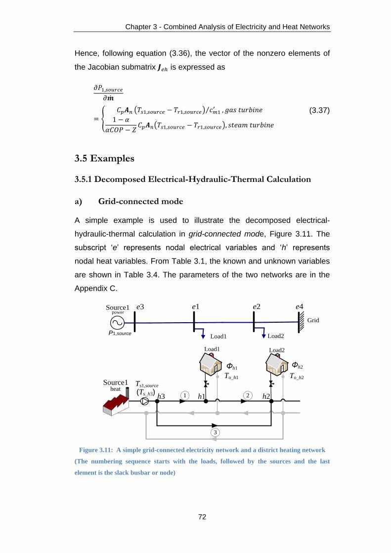
Chapter 3 - Combined Analysis of Electricity and Heat Networks
72
Hence, following equation (3.36), the vector of the nonzero elements of
the Jacobian submatrix is expressed as
(3.37)
3.5 Examples
3.5.1 Decomposed Electrical-Hydraulic-Thermal Calculation
a) Grid-connected mode
A simple example is used to illustrate the decomposed electrical-
hydraulic-thermal calculation in grid-connected mode, Figure 3.11. The
subscript ‘e’ represents nodal electrical variables and ‘h’ represents
nodal heat variables. From Table 3.1, the known and unknown variables
are shown in Table 3.4. The parameters of the two networks are in the
Appendix C.
Source1power
Grid
e1 e2e3 e4
Load1 Load2P1,source
Load2
h3 h1 h2
Source1
Load1
Load2
To_h1 To_h2
Ts1,source
Φh1 Φh2
heat1 2
3
(Ts_h3)
Figure 3.11: A simple grid-connected electricity network and a district heating network
(The numbering sequence starts with the loads, followed by the sources and the last
element is the slack busbar or node)
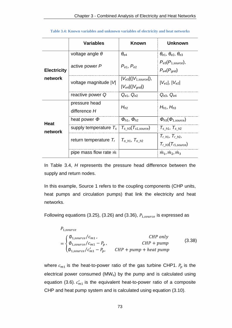
Chapter 3 - Combined Analysis of Electricity and Heat Networks
73
Table 3.4: Known variables and unknown variables of electricity and heat networks
Variables Known Unknown
Electricity
network
voltage angle θ θe4 θe1, θe2, θe3
active power P Pe1, Pe2 Pe3(P1,source),
Pe4(Pgrid)
voltage magnitude |V| |Ve3|(|V1,source|),
|Ve4|(|Vgrid|) |Ve1|, |Ve2|
reactive power Q Qe1, Qe2 Qe3, Qe4
Heat
network
pressure head
difference H Hh2 Hh1, Hh3
heat power Φ Φh1, Φh2 Φh3(Φ1,source)
supply temperature Ts Ts_h3(Ts1,source) Ts_h1, Ts_h2
return temperature Tr To_h1, To_h2 Tr_h1, Tr_h2,
Tr_h3(Tr1,source)
pipe mass flow rate
In Table 3.4, H represents the pressure head difference between the
supply and return nodes.
In this example, Source 1 refers to the coupling components (CHP units,
heat pumps and circulation pumps) that link the electricity and heat
networks.
Following equations (3.25), (3.26) and (3.36), is expressed as
(3.38)
where is the heat-to-power ratio of the gas turbine CHP1. is the
electrical power consumed (MWe) by the pump and is calculated using
equation (3.6). is the equivalent heat-to-power ratio of a composite
CHP and heat pump system and is calculated using equation (3.10).

Chapter 3 - Combined Analysis of Electricity and Heat Networks
74
For the heat supply network as shown in Figure 3.11, the network
incidence matrix A and the loop incidence matrix B are:
A =
B =
Following Figure 3.9, for the example networks in grid-connected mode,
steps 1) – 10) used to solve the example networks linked by a CHP unit
only are as follows
1) The calculation starts with the known heat and electrical variables as
shown in Table 3.5. The known heat variables are labelled in Figure
3.11.
Table 3.5: Known variables for the example networks
Known heat variables
· Heat power of each heat load:Φh1 = Φh2 = 0.3MWth
· Supply temperature of Source 1: Ts1,source = 100°C
· Outlet temperature (return temperature before mixing) of
each heat load: To_h1 = To_h2 = 50°C
Known electrical variables
· Active power of each electrical load: Pe1 = Pe2 = 0.15MWe
· Power factor of each electrical load: p.f. = 0.95, thus Qe1 =
Qe2 = 0.0493MVar
· Voltage magnitude of Source 1 and Grid: |V1,source| = |Ve3| =
1.05p.u., |Vgrid| = |Ve4| = 1.02p.u.
· Voltage angle of Grid: θgrid = θe4 = 0°
2) Assume the initial conditions for the heat and electricity networks are
as follows:
1 2 3
1 1 1 -1
Loop N
o.
Pipe No. 1 2 3
1 1 -1 0
2 0 1 1
Node N
o.
Pipe No.

Chapter 3 - Combined Analysis of Electricity and Heat Networks
75
Heat:
,
.
Electricity:
.
3) Calculate the nodal mass flow rates using the heat power
equation (2.27). For the first iteration
4) Hydraulic calculation
Update the pipe mass flow rates based on using the
hydraulic model.
a) Calculate the hydraulic mismatches using the flow
continuity equation (2.3) and the loop pressure equation (2.8)
For the first iteration
b) Hence, the hydraulic Jacobian matrix is

Chapter 3 - Combined Analysis of Electricity and Heat Networks
76
For the first iteration
c) Update the pipe mass flow rates
5) Thermal calculation
Calculate the nodal temperatures using the temperature drop
equation (2.29) and the temperature mixing equation (2.30).
a) Calculate
based on and the known
.
where ,
.
b) Calculate
based on and the known .
c) Calculate
based on and
.

Chapter 3 - Combined Analysis of Electricity and Heat Networks
77
6) The procedure of this decomposed hydraulic-thermal calculation is
repeated from step 3) until the maximal , and
become less than ε = 10-3.
After 4 iterations, the converged results of the variables (pipe mass
flow rates and temperatures) of the heat network are:
.
7) Calculate the heat power generated from Source 1.
· Firstly, calculating based on from Step 6)
· Then, substituting and from Step 6) into the
heat power equation (2.27) to obtain
Thus, the heat power losses in the heat network are:
.
8) Calculate the electrical power generated from Source 1 using
equation (3.38), .
9) Electrical power flow calculation
a) Calculate the electrical mismatches
. For the first
iteration,

Chapter 3 - Combined Analysis of Electricity and Heat Networks
78
b) Hence, the electrical Jacobian matrix
is:
9.8056 -4.7832 -5.0224 5.3231 -2.7298
-4.7832 9.6621 0.0000 -2.7298 5.4050
-5.0224 0.0000 5.0224 -2.8663 0.0000
-5.5961 2.7298 2.8663 9.3273 -4.7832
2.7298 -5.5142 0.0000 -4.7832 9.4708
c) Update the state variables (voltage magnitudes and angles)
d) After 3 iterations, the converged results of the state variables
(voltage magnitudes and angles) of the electricity network are:
where the unit of voltage angle is ‘deg’ and the unit of voltage
magnitude is p.u.
The results of the electrical power flow calculation is validated
using IPSA and MATLAB toolbox MATPOWER [96, 97].
10) Calculate the electrical power generated from Grid,
.
Chapter 3 - Combined Analysis of Electricity and Heat Networks
79
Thus, the electrical power losses in the electricity network are:
.
Steps 11) and 12) in Figure 3.9 are only applicable to the example in
islanded mode, which will be discussed in the next section.
In the case of different coupling components, step 8) varies as follows
· CHP and circulation pump
Following equation (3.38)
where the electrical power consumed by the pump is calculated
using equation (3.6)
where the pump head is calculated using equation (3.7)
where Hc is the minimum allowable head differential (m) which refers
to Hh2 in the network shown in Figure 3.11.
· CHP, circulation pump and heat pump
Following equation (3.38)
where the equivalent heat-to-power ratio of a composite CHP and
heat pump system is calculated using equation (3.10).
where α is the percentage of a fraction of electrical power from the
CHP unit modulated to drive the heat pump.
In all three cases, the results of the variables (pipe mass flow rates and
temperatures) of the heat network are the same. The results of the
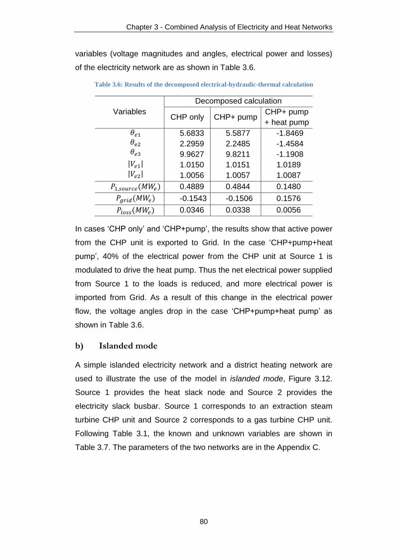
Chapter 3 - Combined Analysis of Electricity and Heat Networks
80
variables (voltage magnitudes and angles, electrical power and losses)
of the electricity network are as shown in Table 3.6.
Table 3.6: Results of the decomposed electrical-hydraulic-thermal calculation
Variables
Decomposed calculation
CHP only CHP+ pump CHP+ pump
+ heat pump
5.6833
2.2959
9.9627
1.0150
1.0056
5.5877
2.2485
9.8211
1.0151
1.0057
-1.8469
-1.4584
-1.1908
1.0189
1.0087
0.4889 0.4844 0.1480
-0.1543 -0.1506 0.1576
0.0346 0.0338 0.0056
In cases ‘CHP only’ and ‘CHP+pump’, the results show that active power
from the CHP unit is exported to Grid. In the case ‘CHP+pump+heat
pump’, 40% of the electrical power from the CHP unit at Source 1 is
modulated to drive the heat pump. Thus the net electrical power supplied
from Source 1 to the loads is reduced, and more electrical power is
imported from Grid. As a result of this change in the electrical power
flow, the voltage angles drop in the case ‘CHP+pump+heat pump’ as
shown in Table 3.6.
b) Islanded mode
A simple islanded electricity network and a district heating network are
used to illustrate the use of the model in islanded mode, Figure 3.12.
Source 1 provides the heat slack node and Source 2 provides the
electricity slack busbar. Source 1 corresponds to an extraction steam
turbine CHP unit and Source 2 corresponds to a gas turbine CHP unit.
Following Table 3.1, the known and unknown variables are shown in
Table 3.7. The parameters of the two networks are in the Appendix C.

Chapter 3 - Combined Analysis of Electricity and Heat Networks
81
Source1power
Source2powere1 e2e3 e4
Load1 Load2
5
Load2
h4
h1 h2
Source1
Load1
Load2
To_h1 To_h2
Ts1,source
To_h3
Ts2,source
h3
h5
1
4
2 3
Source2heat heat
Load3
Figure 3.12: A simple islanded electricity network and a district heating network
(The numbering sequence starts with the loads, followed by the sources and the last
element is the slack busbar or node)
Table 3.7: Known variables and unknown variables of electricity and heat networks
Variables Known Unknown
Electricity
network
voltage angle θ θe4 θe1, θe2, θe3
active power P Pe1, Pe2 Pe3(P1,source),
Pe4(P2,source)
voltage
magnitude |V|
|Ve3|(|V1,source|),
|Ve4|(|V2,source|) |Ve1|, |Ve2|
reactive power Q Qe1, Qe2 Qe3, Qe4
Heat
network
pressure head H Hh2 Hh1, Hh3, Hh4, Hh5
heat power Φ Φh1, Φh2, Φh3 Φh4(Φ1,source),
Φh5(Φ2,source)
supply
temperature Ts
Ts_h4(Ts1,source),
Ts_h5(Ts2,source) Ts_h1, Ts_h2, Ts_h3
return
temperature Tr To_h1, To_h2, To_h3
Tr_h1, Tr_h2, Tr_h3,
Tr_h4(Tr1,source),
Tr_h5(Tr2,source)
mass flow rate

Chapter 3 - Combined Analysis of Electricity and Heat Networks
82
In this example, Source 1 and Source 2 refer to the coupling components
(CHP units, heat pumps and circulation pumps) that link the electricity
and heat networks.
Following from equations (3.25), (3.26) and (3.36), for the extraction
steam turbine CHP unit at Source 1, is expressed as
(3.39)
In the case ‘CHP+pump+heat pump’, a heat pump is connected to the
CHP unit at Source 1 in cascade and fed by cogenerated electricity.
Following from equations (3.25) and (3.26), for the gas turbine CHP unit
at Source 2, is expressed as
(3.40)
For the heat supply network shown in Figure 3.12, the network incidence
matrix A and the loop incidence matrix B are
A =
B =
The procedure used to illustrate the use of the model is through
determining the heat and electrical power generated from Source 1 and
Source 2 at each iteration, Figure 3.13. This Figure illustrates the steps
7, 8, 10, 11 in the flowchart as shown in Figure 3.9. In Figure 3.13, the
1 2 3 4 5
1 1 -1 -1 1 -1
Loop N
o.
Pipe No.
1 2 3 4 5
1 1 1 0 0 0
2 0 -1 1 0 0
3 0 0 0 1 1
4 0 0 -1 -1 0
5 -1 0 0 0 -1
Pipe No.
Node N
o.

Chapter 3 - Combined Analysis of Electricity and Heat Networks
83
left line that slopes downward describes the performance curve of an
extraction steam turbine CHP unit at Source 1 and the slope is equal to
the negative of the Z ratio of Source 1 (-Z). The right line that slopes
upward describes the performance curve of a gas turbine CHP unit at
Source 2 and the slope is equal to the heat-to-power ratio of Source 2
( ).
0.2 0.21 0.22 0.23 0.24 0.25
0.2
0.25
0.3
0.35
Heat
pow
er
(MW
th)
Electrical power (MWe)
Source 2
0.08 0.085 0.09
0.65
0.7
Heat
pow
er
(MW
th)
Electrical power (MWe)
3
3
4
2
3
1
Source 1b
d
f
c
e
P1,source
Φ1,source
starta
gend
(2)(3)P1,source
(1)P2,source
Φ1,source
Φ1,source
(2)
(3)
(1)
P2,source
(2)
(3)P2,source
Φ2,source
Φ2,source
Φ2,source
(2)
(3)
(1)
P1,source(1)
Figure 3.13: Procedure to calculate the electrical and heat power from both Source 1 and
Source 2 that link electricity and heat networks
Following Figure 3.9, the steps used to solve the model for the example
networks linked by a CHP unit only are as follows
1) Start with the known variables as shown in Table 3.7.
2) Assume the initial conditions for the heat and electricity networks are
as follows:
Heat:
,
.
.
Electricity:
.

Chapter 3 - Combined Analysis of Electricity and Heat Networks
84
Iteration i = 1.
3-6) Solve the hydraulic and thermal model, represented in Figure 3.13
as the red dashed arrow a→b when i = 1.
7) Calculate
, represented in Figure 3.13 as a horizontal dotted
line.
8) Calculate
, represented in Figure 3.13 as a vertical dotted line,
according to the performance curve of Source 1 using equation
(3.39).
9) Solve the electrical power flow model, represented in Figure 3.13 as
the blue solid arrow b→c when i = 1.
10) Calculate
, represented in Figure 3.13 as a vertical solid line.
11) Calculate
, represented in Figure 3.13 as a horizontal solid
line, according to the performance curve of Source 2 using equation
(3.40).
12) This procedure is repeated from step 3 until
becomes less than the tolerance ε. i = i + 1.
The number of iterations for the hydraulic and thermal model and the
electrical power flow model is shown in Table 3.8. After 16 total iterations
(3 + 3 + 4 + 2 + 3 + 1 = 16), the results converged.
Table 3.8: Number of iterations in the hydraulic and thermal and electrical models
Model
Hydraulic
and
thermal
Electrical
Hydraulic
and
thermal
Electrical
Hydraulic
and
thermal
Electrical
a → b b → c c → d d → e e → f f → g
No. of
iterations 3 3 4 2 3 1
In the case of different coupling components, the results of the variables
of the electricity and heat networks are shown in Table 3.9.

Chapter 3 - Combined Analysis of Electricity and Heat Networks
85
Table 3.9: Results of the decomposed electrical-hydraulic-thermal calculation
Variables
Decomposed calculation
CHP only CHP+pump CHP+pump +heat pump
1.0186 1.0186 1.0183
1.0083 1.0082 1.0079
-3.3541 -3.4494 -4.0351
-2.2118 -2.2595 -2.5522
-3.4214 -3.5624 -4.4287
1.7705 1.7605 1.7083
-0.3075 -0.2973 -0.2443
1.2004 1.2104 1.2623
0.1622 0.1840 0.2957
1.3392 1.3176 1.2065
99.0328 99.0273 98.9978
97.5749 97.5812 97.6164
97.7798 97.7728 97.7532
49.5810 49.5790 49.5692
50.0000 50.0000 50.0000
50.0000 50.0000 50.0000
48.9132 48.9343 49.0370
49.2749 49.2678 49.2288
0.6597 0.6531 0.6189
0.0840 0.0847 0.0601
0.2920 0.2976 0.3319
0.2246 0.2310 0.2577
0.0087 0.0111 0.0134
0.0517 0.0506 0.0508
Based on Table 3.9, the bar chart in Figure 3.14 is used to show the heat
and electrical power supplied from two sources. The electrical (heat)
network losses are expressed as the differences between the sum of the
electrical (heat) power of two sources and total electrical (heat) loads.

Chapter 3 - Combined Analysis of Electricity and Heat Networks
86
Figure 3.14: Electrical and heat power supplied from two sources
3.5.2 Integrated Electrical-Hydraulic-Thermal Calculation
a) Grid-connected mode
To illustrate the integrated electrical-hydraulic-thermal calculation in grid-
connected mode, the model equations are applied to the electricity and
heat networks shown in Figure 3.11.
Following equation (3.31), the state variables are
(3.41)
Following equation (3.32), the vector of total mismatches ∆F for the
electricity and heat networks shown in Figure 3.11 are
Source 1 0.0840
Source 1 0.6597
Source 2 0.2246
Source 2 0.2920
Load 0.3
Load 0.9
0
0.1
0.2
0.3
0.4
0.5
0.6
0.7
0.8
0.9
1
0
0.1
0.2
0.3
0.4
0.5
0.6
0.7
0.8
0.9
1
Electricity Heat
Source 2
Source 1
Load
Ele
ctric
al p
ow
er (M
We )
Heat p
ow
er (M
Wth )

Chapter 3 - Combined Analysis of Electricity and Heat Networks
87
(3.42)
where Real represents the real part of a complex expression and Imag
represents the imaginary part of a complex expression. Following
equations (3.24), (3.25), (3.26) and (3.36),
in the 3rd row of ∆F is a
function of the heat network and is expressed as
(3.43)
The steps used to solve the integrated electrical-hydraulic-thermal
calculation for the example networks shown in Figure 3.11 linked by a
CHP unit only are as follows
a) Assume the initial condition as,
b) Calculate the mismatches . For the first iteration,
…

Chapter 3 - Combined Analysis of Electricity and Heat Networks
88
,
c) Hence, the Jacobian matrix is:
d) Update the state variables. For the first iteration,
.
e) The procedure is repeated until the maximum absolute value of
elements in the mismatches becomes less than the tolerance ε =
10-3.
After 5 iterations, the converged results of the variables of the
networks are:
,
Tr1,source = 49.1252.
.
9.806 -4.783 -5.022 5.323 -2.730
-4.783 9.662
-2.730 5.405
-5.022
5.022 -2.866
-0.277
-0.277
-5.596 2.730 2.866 9.327 -4.783
2.730 -5.514
-4.783 9.471
0.209 -0.209
0.209 0.209
0.008
0.036 0.036 -0.054
1.000
-0.981 2.000
1.000 -0.981
1.000

Chapter 3 - Combined Analysis of Electricity and Heat Networks
89
In the case of different coupling components, the results of the variables
(pipe mass flow rates and temperatures) of the heat network are the
same. The results of the variables (voltage magnitudes and angles,
electrical power and losses) of the electricity network are as shown in
Table 3.10.
Table 3.10: Results of the integrated electrical-hydraulic-thermal calculation
Variables
Integrated calculation
CHP only CHP + pump CHP + pump + heat pump
5.6831 2.2958 9.9625 1.0150 1.0056
5.5875 2.2484 9.8210 1.0151 1.0057
-1.8469 -1.4584 -1.1909 1.0189 1.0087
0.4889 0.4843 0.1480
-0.1543 -0.1506 0.1576
0.0346 0.0338 0.0056
b) Islanded mode
To illustrate the use of the model in islanded mode, the model equations
are applied to the electricity and heat networks shown in Figure 3.12.
The procedure used to illustrate the example networks linked by a CHP
unit only is shown in Figure 3.15. During each iteration, the electrical and
heat power generated from two sources are obtained simultaneously,
which are represented as the points on the performance curves (the left
line that slopes downward and the right line that slopes upward) of two
CHP units. Due to the scale of the graph, starting from the 6th points on
two lines, the two points on two lines are then simultaneously moved to
the next two points with the same index at each iteration. The iteration
procedure is repeated until the maximum absolute value of elements in
the mismatches becomes less than the tolerance ε = 10-3. After 12
iterations, the results converged.

Chapter 3 - Combined Analysis of Electricity and Heat Networks
90
0.08 0.081 0.082 0.083 0.084 0.0850.65
0.66
0.67
0.68
0.69
0.7
He
at p
ow
er
(MW
th)
Electric power (MWe)
1
2
3
4
5
5
67
8 9101112
Source 1
0.224 0.225 0.226 0.2270.29
0.295
0.3
He
at p
ow
er
(MW
th)
Electric power (MWe)
Source 2
6
7
910,11,12
6
7
8910
11,128
Figure 3.15: Procedure to calculate the electrical and heat power from both Source 1 and
Source 2 that link electricity and heat networks
Following from equations (3.25), (3.26) and (3.36), for the extraction
steam turbine CHP unit at Source 1, is expressed as
(3.44)
where
.
In the case ‘CHP+pump+heat pump’, a heat pump is connected to the
CHP unit at Source 1 in cascade and fed by cogenerated electricity.
Following from equations (3.25) and (3.26), for the gas turbine CHP unit
at Source 2, is expressed as
(3.45)
where .
In the case of different coupling components, the results of the variables
of the electricity and heat networks are shown in Table 3.11.

Chapter 3 - Combined Analysis of Electricity and Heat Networks
91
Table 3.11: Results of the integrated electrical-hydraulic-thermal calculation
Variables
Integrated calculation
CHP only CHP + pump CHP + pump + heat pump
1.0186 1.0186 1.0183
1.0083 1.0082 1.0079
-3.3523 -3.4439 -4.0303
-2.2109 -2.2567 -2.5498
-3.4187 -3.5542 -4.4216
1.7693 1.7571 1.7043
-0.3063 -0.2939 -0.2401
1.2016 1.2137 1.2663
0.1648 0.1912 0.3042
1.3367 1.3105 1.1981
99.0321 99.0257 98.9953
97.5757 97.5831 97.6195
97.7787 97.7710 97.7522
49.5807 49.5785 49.5684
50.0000 50.0000 50.0000
50.0000 50.0000 50.0000
48.9160 48.9406 49.0449
49.2740 49.2655 49.2253
0.6589 0.6509 0.6163
0.0841 0.0849 0.0603
0.2919 0.3000 0.3347
0.2245 0.2308 0.2575
0.0087 0.0110 0.0134
0.0508 0.0509 0.0510
The differences of the results of the cases ‘CHP only’ and ‘CHP+pump’
are not significant, which means the impact of the circulation pump to the
interaction of two networks is small. In the case ‘CHP+pump+heat
pump’, 40% of the electrical power from the CHP unit at Source 1 is
modulated to drive the heat pump. Thus the net electrical power supplied
from Source 1 to the loads is reduced, and more electrical power is
supplied from Source 2. As a result of this change in the electrical power
flow, the voltage angles drop in the case ‘CHP+pump+heat pump’ as
shown in Table 3.11.
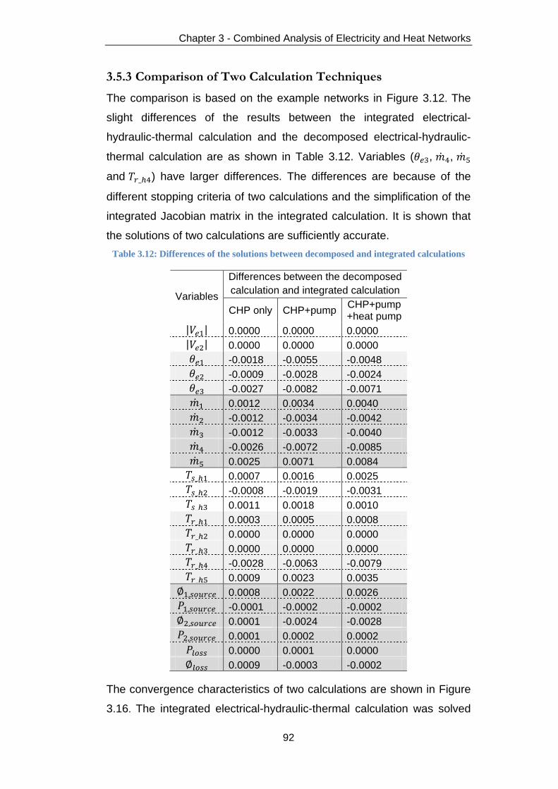
Chapter 3 - Combined Analysis of Electricity and Heat Networks
92
3.5.3 Comparison of Two Calculation Techniques
The comparison is based on the example networks in Figure 3.12. The
slight differences of the results between the integrated electrical-
hydraulic-thermal calculation and the decomposed electrical-hydraulic-
thermal calculation are as shown in Table 3.12. Variables ( , ,
and ) have larger differences. The differences are because of the
different stopping criteria of two calculations and the simplification of the
integrated Jacobian matrix in the integrated calculation. It is shown that
the solutions of two calculations are sufficiently accurate.
Table 3.12: Differences of the solutions between decomposed and integrated calculations
Variables
Differences between the decomposed
calculation and integrated calculation
CHP only CHP+pump CHP+pump +heat pump
0.0000 0.0000 0.0000
0.0000 0.0000 0.0000
-0.0018 -0.0055 -0.0048
-0.0009 -0.0028 -0.0024
-0.0027 -0.0082 -0.0071
0.0012 0.0034 0.0040
-0.0012 -0.0034 -0.0042
-0.0012 -0.0033 -0.0040
-0.0026 -0.0072 -0.0085
0.0025 0.0071 0.0084
0.0007 0.0016 0.0025
-0.0008 -0.0019 -0.0031
0.0011 0.0018 0.0010
0.0003 0.0005 0.0008
0.0000 0.0000 0.0000
0.0000 0.0000 0.0000
-0.0028 -0.0063 -0.0079
0.0009 0.0023 0.0035
0.0008 0.0022 0.0026
-0.0001 -0.0002 -0.0002
0.0001 -0.0024 -0.0028
0.0001 0.0002 0.0002
0.0000 0.0001 0.0000
0.0009 -0.0003 -0.0002
The convergence characteristics of two calculations are shown in Figure
3.16. The integrated electrical-hydraulic-thermal calculation was solved

Chapter 3 - Combined Analysis of Electricity and Heat Networks
93
in 12 iterations and the decomposed electrical-hydraulic-thermal
calculation was solved in 16 iterations. The integrated calculation
achieves fewer iterations than the decomposed calculation, because the
set of equations is solved as a whole using the Newton-Raphson
method, providing quadratic convergence with respect to time. However,
the integrated calculation requires more computations per iteration than
the decomposed calculation. In the decomposed calculation, the
electrical power flow equations and the hydraulic and thermal model
equations are solved individually, hence this method requires more
iterations.
Figure 3.16: Convergence characteristics of the decomposed and integrated electrical-
hydraulic-thermal calculations
1 2 3 4 5 6 7 8 9 10 11 12 13 14 15 160
0.05
0.1
0.15
0.2
0.25
0.3
0.35
0.4
0.45
Iteration
Mis
matc
hes
Decomposed model (Heat part)
Decomposed model (Electricity part)
Integrated model

Chapter 3 - Combined Analysis of Electricity and Heat Networks
94
3.6 Summary
The use of CHP units and heat pumps increases the linkages between
electricity and heat networks. A combined analysis was developed to
investigate the performance of electricity and heat networks as an
integrated whole. This was based on a model of electrical power flow
and hydraulic and thermal circuits together with their coupling
components elements (CHP units, heat pumps, electric boilers and
circulation pumps). The combined analysis took into account the flows of
energy between the electricity and heat networks through the coupling
components.
Two calculation techniques (decomposed and integrated electrical-
hydraulic-thermal calculations) were developed. Three combinations of
coupling mechanisms (CHP only; CHP and circulation pump; CHP,
circulation pump and heat pump) were considered in each calculation.
The calculations were demonstrated in grid-connected and islanded
operation modes.
In grid-connected mode, any surplus or deficit in electrical power is
supplied from the main grid and not from the CHP units, thus there is no
linkage back from the electrical system to the heat system. While in
islanded mode there are bidirectional linkages between the electricity
and heat networks.
For the decomposed electrical-hydraulic-thermal calculation in grid-
connected mode, the hydraulic and thermal model was solved first. Then
these results were transferred to the electricity network through the
coupling components. Finally the electrical power flow model was solved.
In islanded mode, this sequential procedure was iterated until the
solution converged to an acceptable tolerance.
For the integrated electrical-hydraulic-thermal calculation, the electrical
power flow equations, the hydraulic equations and the thermal equations
were combined to form a single system of equations and solved
simultaneously as an integrated whole using the Newton-Raphson
method.

Chapter 3 - Combined Analysis of Electricity and Heat Networks
95
Using the combined analysis, the variables of the electrical and heat
networks were calculated. These included: heat and electrical power
from the CHP units, mass flow rates, supply and return temperatures,
voltage magnitudes and voltage angles, heat and electrical power
losses.
The results of the decomposed and integrated calculations were very
close to 10-3 precision. The real values were used in the calculation of
heat networks and the per unit was used in the calculation of electrical
networks. The convergence characteristics of two calculations were
compared. The comparison showed that the integrated calculation
requires fewer iterations than the decomposed calculation. In a simple
example network, the decomposed calculation was solved in 16
iterations and the integrated calculation was solved in 12 iterations.
The combined analysis can be used for the design and operation of
integrated heat and electricity systems for energy supply to buildings.
This will increase the flexibility of the electricity and heat supply systems
for facilitating the integration of intermittent renewable energy.

Chapter 4 - Case Study
4.1 Introduction
The linkage between the electricity and heat networks is formed by
coupling components with unknown electrical and heat power. The
coupling components can be CHP units, heat pumps and electric boilers.
The schematic diagram for the linkages is shown in Figure 4.1. The
electrical and heat power generated from all sources, except the slack
busbar or node, are known, there is one linkage in grid-connected mode
and two linkages in islanded mode through the slack busbar or node.
Electricity
Heat
Electricity
Unknown heat and
electrical power
…
District heating network
Electric power distribution networkElectricity
slack
busbar
HeatHeat
slack
node
Electricity Electricity
Heat Heat
Linkages
Source 2 Source N-1Source 1 …
…
Source N
Unknown heat and
electrical power
Known heat and
electrical power
Known heat and
electrical power
Figure 4.1: Linkages between electricity and district heating networks
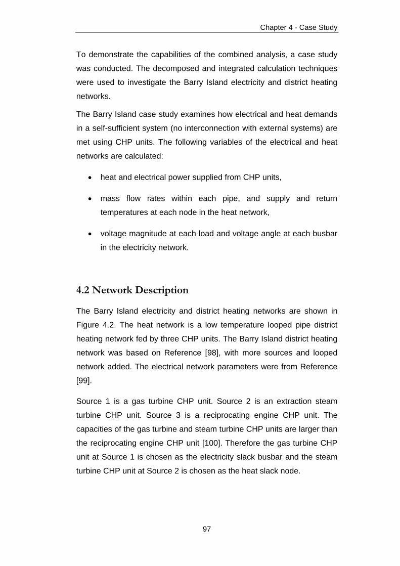
Chapter 4 - Case Study
97
To demonstrate the capabilities of the combined analysis, a case study
was conducted. The decomposed and integrated calculation techniques
were used to investigate the Barry Island electricity and district heating
networks.
The Barry Island case study examines how electrical and heat demands
in a self-sufficient system (no interconnection with external systems) are
met using CHP units. The following variables of the electrical and heat
networks are calculated:
· heat and electrical power supplied from CHP units,
· mass flow rates within each pipe, and supply and return
temperatures at each node in the heat network,
· voltage magnitude at each load and voltage angle at each busbar
in the electricity network.
4.2 Network Description
The Barry Island electricity and district heating networks are shown in
Figure 4.2. The heat network is a low temperature looped pipe district
heating network fed by three CHP units. The Barry Island district heating
network was based on Reference [98], with more sources and looped
network added. The electrical network parameters were from Reference
[99].
Source 1 is a gas turbine CHP unit. Source 2 is an extraction steam
turbine CHP unit. Source 3 is a reciprocating engine CHP unit. The
capacities of the gas turbine and steam turbine CHP units are larger than
the reciprocating engine CHP unit [100]. Therefore the gas turbine CHP
unit at Source 1 is chosen as the electricity slack busbar and the steam
turbine CHP unit at Source 2 is chosen as the heat slack node.

Chapter 4 - Case Study
98
201.3
m
1
257.6 m
97
.5 m
59.5 m
51 m271.3 m
235.4
m
177.
3 m
102.
8 m
247.7 m
160.
8 m
129.1 m18
6.1
m
136.2 m
41.8
m
116.8 m 136.4 m
136.4 m
44
.9 m
41.7
m5
2.1
m6
1.8
m
136.4 m 134.1 m
134.2 m161.1 m
123.3 m136 m
105.1 m95.2 m
2
3
4
5
6
7
8
9
10
11
12
13
14
15 1716
18
1920 21
23 24
2726
3029
22
25
28
70.6
261.8 m
1
2
3
31
Source
(heat) Pump Heat load Pipeline
4
510
6
7
8
31
2928
2625
2322
2019
1317
15 16
12
9
11
30
27
24
21
18
14
320m230m
260m
260m
170m
160m
Source
(electricity)
Source 1power heat
Source 2
power
heat
Electrical load Electrical line
vi
iv
v
iii
ii
i
vii
ix
Source 3power heat
viii
200m
32
32
Figure 4.2: Schematic diagram of the electricity and district heating networks of the Barry Island case study

Chapter 4 - Case Study
99
4.2.1 Electricity Network
The schematic diagram of the electric power distribution network is
shown in Figure 4.3. The electrical power is supplied to 5 lumped
electrical loads through a 11/0.433kV transformer at each feeder. Source
1 is connected to the 11kV distribution network through a 33/11.5kV
transformer. Busbar ix is the slack busbar.
8
9
10
30
29
26
27
23
24
16
17
14
18
20
21
6
11
12
3
4
100m
50m
270m
160m
290m
120m
140m
40m
180m
220m
220m
105m
95m
200m
180m
270m
240m
180m
100m
250m
vii
320m230m260m
11/0.433kV
260m170m
viviviiiii
160m
11/0.433kV11/0.433kV11/0.433kV11/0.433kV
i
Source 2power
Source 1power
Load numbered in the heat network
Lumped electrical load
0.2MWe
0.5MWe 0.5MWe
0.2MWe
0.2MWe
ix
33/11.5kV
Source 3power
viii
200m
Figure 4.3: Schematic diagram of the electric power distribution network of the Barry
Island case study
For the electricity network, the following assumptions were made:
· The base apparent power is 1MVA and base voltage is 11kV.
· The impedance of 185mm2 Cable is 0.164 + j0.080Ω/km [99].
· 33/11.5kV 15MVA transformer has an impedance of 18% and X/R
ratio of 15 [99].
· Active power of 5 lumped electrical loads at each load busbar:
Pi = 0.2MWe,
Piii = 0.5MWe,

Chapter 4 - Case Study
100
Piv = 0.5MWe,
Pv = 0.2MWe,
Pvi = 0.2MWe.
· Power factor of each electrical load: p.f. = 1.
· Voltage magnitude of each Source:
|V1,source| = 1.02p.u.,
|V2,source| = 1.05p.u.,
|V3,source| = 1.05p.u.
· Voltage angle of Source 1: θ1,source = 0°.
The input data of the units of the electrical system were converted into
per unit:
· For the impedance of each cable:
Taking the cable i-ii as an example, the length is 260m, thus the
impedance of the cable is
.
The base impedance is
, thus the impedance of
the cable is
· For the impedance of the 33/11.5kV transformer:
The transformer is 15MVA and the system base apparent power is
1MVA, thus the reactance of the transformer is Xtrans = 18%/15 =
0.012p.u.
The X/R ratio is 15, thus the resistance of the transformer is Rtrans =
0.012/15 = 0.0008p.u.
· For active power at each load busbar:

Chapter 4 - Case Study
101
The base apparent power is 1MVA, thus
Pi = 0.2p.u.,
Piii = 0.5p.u.,
Piv = 0.5p.u.,
Pv = 0.2p.u.,
Pvi = 0.2p.u.
4.2.2 Heat Network
The schematic diagram of the heat network is shown in Figure 4.4. The
pipe parameters are presented in the Appendix D.
1
257.6m
97
.5m
59.5m
51m
271.3m
235.4
m
177.
3m
102.
8m
247.7m
160.
8m
129.1m
186.
1m
136.2m
41
.8m
116.8m 136.4m
136.4m
44
.9m
41
.7m
52
.1m
61
.8m
136.4m 134.1m
134.2m161.1m
123.3m136m
105.1m95.2m
2
3
4
5
6
7
8
9
10
11
12
13
14
15 1716
18
1920 21
23 24
2726
3029
22
25
28
70
.6
261.8m
1
2
3
31
Source
(heat)
Pump
Heat load
Pipeline
4
510
6
7
8
31
2928
2625
2322
2019
1317
15 16
12
9
11
30
27
24
21
18
14
Source1heat
Source2heat
0.107MWth
0.145MWth
0.107MWth0.0805MWth
0.145MWth
0.107MWth
0.107MWth
0.0805MWth
0.0805MWth
0.0805MWth 0.0805MWth
0.107MWth
0.107MWth
0.107MWth0.107MWth
0.107MWth
0.107MWth 0.107MWth
0.107MWth
0.0805MWth
0.107MWth
201.3
m
Source 3heat
32
32
Figure 4.4: Schematic diagram of the heat network of the Barry Island case study
It was assumed that the heat power of the loads is known. The data of
the heat power of the loads (MWth) are shown in Figure 4.4. The total
heat power of the loads is 2.164MWth. Node 1, node 11 and node 31
correspond to three sources. Node 1 is the heat slack node.
It was assumed that:
· Supply temperature at each source: Ts,source = 70°C.

Chapter 4 - Case Study
102
· Outlet temperature (return temperature before mixing) at each
heat load: To,load = 30°C.
4.2.3 CHP Units
For the gas turbine CHP unit at Source 1, the relation between the heat
and electrical power generation was calculated using the equation:
(4.1)
where is the heat-to-power ratio, [89, 90]. ΦCHP1 (MWth) is
the useful heat output. PCHP1 (MWe) is the electrical power output. Both
variables are unknown in this case study.
For the extraction steam turbine CHP unit at Source 2, the Z ratio was
used to calculate the heat output [94]:
(4.2)
where is the Z ratio, [94]. is the increased heat recovery
and is reduced electrical power output. ΦCHP2 (MWth) is the useful
heat output. PCHP2 (MWe) is the electrical power output. Both variables
are unknown in this case study. is the electrical power generation
of the extraction unit in full condensing mode. In this mode, the heat
generation is zero, thus . In this case study, .
For the reciprocating engine CHP unit at Source 3, the relation between
the heat and electrical power generation was calculated using the
equation:
(4.3)
where is the heat-to-power ratio, [90]. ΦCHP3 (MWth) is
the useful heat output. PCHP3 (MWe) is the electrical power output.

Chapter 4 - Case Study
103
4.3 Calculations
In the case study, the heat and electrical power generated from Source 1
and Source 2 are unknown. The heat and electrical power generated
from non-slack Source 3 are known (Table 4.1). It is assumed that the
electrical power generated from Source 3 is . Its
calculated heat power is .
Table 4.1: Heat and electrical power from three sources
Source 1
(electricity slack
busbar)
Source 2
(heat slack
node)
Source 3
(non-
slack)
Heat power Unknown Unknown Known
Electrical power Unknown Unknown Known
Heat-to-power ratio or
Z ratio Known Known Known
The number of the state variables for the case study is shown in Table
4.2.
· The number of voltage angles ( ) is equal to the number of
busbars minus one.
· The number of voltage magnitude ( ) is equal to the number of
load busbars.
· The number of mass flow rates ( ) is equal to the number of
pipes.
· The number of temperatures ( or ) is equal to the
number of load nodes.
Table 4.2: Number of the state variables for the case study
State variables Total
Number 8 6 32 29 29 104

Chapter 4 - Case Study
104
The following initial conditions for the heat and electricity networks were
assumed:
Heat:
· Supply temperature at each heat load:
· Mass flow rate within each pipe:
· Heat power generated from Source 1:
Electricity:
· Voltage magnitude at each electrical load busbar:
· Voltage angle at each busbar except the slack busbar:
For the heat supply network as shown in Figure 4.4, the network
incidence matrix A was created and is shown in the Appendix E.
The integrated and decomposed electrical-hydraulic-thermal calculations
were used in this case study. The calculation techniques were the same
as described in Chapter 3.
The steps used to solve the integrated calculation are as follows:
1) Initialise variables. Iteration i = 1.
2) Calculate the mismatches .
3) Calculate the Jacobian matrix .
4) Update the state variables using the equation
.
5) The procedure is repeated until the maximum absolute value of
elements in the mismatches becomes less than the tolerance ε =
10-3. i = i + 1.
After 16 iterations, the results converged.

Chapter 4 - Case Study
105
The steps used to solve the decomposed calculation are as follows:
1) Initialise variables. Iteration i = 1.
2) Solve the hydraulic and thermal model to obtain pipe mass flow rates,
supply and return temperatures.
3) Calculate
.
4) Calculate
.
5) Solve the electrical power flow model to obtain voltage magnitudes
and voltage angles.
6) Calculate
.
7) Calculate
.
8) This procedure is repeated until
becomes less than the tolerance ε = 10-3. i = i + 1.
After 33 total iterations, the results converged. The total iterations
consist of the iterations of the electrical power flow model and the
hydraulic and thermal model.
The results of the decomposed and integrated calculations were very
close at 10-3 precision.
4.4 Results
The results of the calculation of the heat and electrical power from
Source 1 and Source 2 are shown in Figure 4.5. The electrical and heat
power network losses are the differences between the sum of the power
supplied from three sources and the electrical and heat loads. The
electrical power network loss is 0.0118MWe (0.74%). The heat network
loss is 0.0809MWth (3.74%).

Chapter 4 - Case Study
106
Figure 4.5: Heat and electrical power supplied from three sources
The results of the calculation of the pipe mass flow rates are shown in
Figure 4.6. In the figure the main flow route 1 – 2 – 5 – 11 – 13 – 14 – 19
– 22 – 25 – 28 – 31 – 7 – 5 is indicated using bold lines. It is seen that in
some pipes ( 6 , 24 and 27) the flows are of opposite direction compared
with the initial guess, as shown in Figure 4.4, and the mass flow rates
are different. The mass flow rate within pipe 12 is increased due to the
flow injection from Source 3. The mass flow rate at node 31 is the largest
since the heat power generated in Source 1 is the largest.
1
4.7977kg/s
3.2708kg/s
0.8
805kg
/s
3.48
48kg
/s
4.1924kg/s
41.8
m2.1
91
3k
g/s
1.1
85
2k
g/s
0.1
52
7k
g/s
1.4
57
5k
g/s
2
3
4
5
6
7
8
9
10
11
12
13
14
15 1716
18
1920 21
23 24
2726
3029
22
25
28
2.7
54
1k
g/s 3.5008kg/s
31
10
6
12
30
27
24
21
18
14
Source1heat
Source2heat
Source 3heat
1
4.7977kg/s
3.2708kg/s
0.8
805kg
/s
3.48
48kg
/s
4.19
24kg
/s
4.1924kg/s
41.8
m2.1
91
3k
g/s
1.1
85
2k
g/s
0.1
52
7k
g/s
1.4
57
5k
g/s
2
3
4
5
6
7
8
9
10
11
12
13
14
15 1716
18
1920 21
23 24
2726
3029
22
25
28
2.7
54
1k
g/s 3.5008kg/s
1
2
3
31
4
5
10
6
7
8
31
2928
2625
2322
2019
1317
15 16
12
9
11
30
27
24
21
18
14
Source1heat
Source2heat
Heat source
Pump
Heat load
Pipeline
Source 3heat
32
Figure 4.6: Results of the pipe mass flow rates (kg/s) in a flow route
0.8118 1.0553
0.5
0.8099 0.3
0.3797
1.6
2.164
0
0.5
1
1.5
2
2.5
0
0.5
1
1.5
2
2.5
Electricity Heat
Source 3
Source 2
Source 1
Load E
lectr
ical pow
er
(MW
e)
Heat
pow
er
(MW
th)

Chapter 4 - Case Study
107
The results of the calculation of the supply and return temperatures at
each node in the main flow route: 1 – 2 – 5 – 11 – 13 – 14 – 19 – 22 – 25
– 28 – 31 – 7 – 5 are shown in Figure 4.7. Node 22 is the end of two flow
streams from Source 1 and Source 2 in the supply network and the start
of the two flow streams in the return network. The lowest supply
temperature and the highest return temperature are at node 22, where
two opposite flow streams meet.
In the main route of the supply network (Figure 4.6), the flows mix at
nodes 5 and 22 only. The supply temperature from node 1 to node 22
reduces gradually because of the heat losses.
In the same route of the return network, the flow mixing occurs at each
node except node 13. Due to the mixing and due to the assumption that
the return temperature from the consumer is fixed, the return
temperature from node 22 to node 1 decreases unevenly.
Figure 4.7: Results of the supply and return temperatures of the nodes in a flow route
The results of the calculation of the voltage magnitude and voltage angle
at each busbar are as shown in Figure 4.8. The voltage angles at source
busbars are lower than those of some load busbars.
1 2 5 11 13 14 19 22 25 28 31 7 568.5
69
69.5
70
Supply
tem
pera
ture
(oC
)
Node number
Supply temperature
1 2 5 11 13 14 19 22 25 28 31 7 529.5
29.6
29.7
29.8
29.9
Node number
Retu
rn t
em
pera
ture
(oC
)
Return temperature
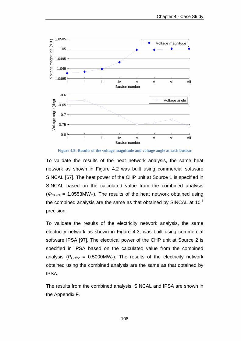
Chapter 4 - Case Study
108
Figure 4.8: Results of the voltage magnitude and voltage angle at each busbar
To validate the results of the heat network analysis, the same heat
network as shown in Figure 4.2 was built using commercial software
SINCAL [67]. The heat power of the CHP unit at Source 1 is specified in
SINCAL based on the calculated value from the combined analysis
(ΦCHP1 = 1.0553MWth). The results of the heat network obtained using
the combined analysis are the same as that obtained by SINCAL at 10-3
precision.
To validate the results of the electricity network analysis, the same
electricity network as shown in Figure 4.3, was built using commercial
software IPSA [97]. The electrical power of the CHP unit at Source 2 is
specified in IPSA based on the calculated value from the combined
analysis (PCHP2 = 0.5000MWe). The results of the electricity network
obtained using the combined analysis are the same as that obtained by
IPSA.
The results from the combined analysis, SINCAL and IPSA are shown in
the Appendix F.
i ii iii iv v vi vii viii1.0485
1.049
1.0495
1.05
1.0505
Voltage m
agnitude (
p.u
.)
Busbar number
Voltage magnitude
i ii iii iv v vi vii viii-0.8
-0.75
-0.7
-0.65
-0.6
Busbar number
Voltage a
ngle
(deg)
Voltage angle
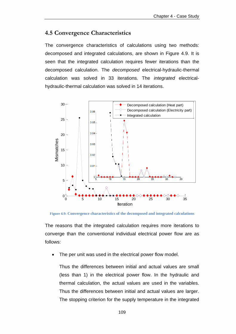
Chapter 4 - Case Study
109
4.5 Convergence Characteristics
The convergence characteristics of calculations using two methods:
decomposed and integrated calculations, are shown in Figure 4.9. It is
seen that the integrated calculation requires fewer iterations than the
decomposed calculation. The decomposed electrical-hydraulic-thermal
calculation was solved in 33 iterations. The integrated electrical-
hydraulic-thermal calculation was solved in 14 iterations.
Figure 4.9: Convergence characteristics of the decomposed and integrated calculations
The reasons that the integrated calculation requires more iterations to
converge than the conventional individual electrical power flow are as
follows:
· The per unit was used in the electrical power flow model.
Thus the differences between initial and actual values are small
(less than 1) in the electrical power flow. In the hydraulic and
thermal calculation, the actual values are used in the variables.
Thus the differences between initial and actual values are larger.
The stopping criterion for the supply temperature in the integrated
0 5 10 15 20 25 30 350
5
10
15
20
25
30
Iteration
Mis
ma
tch
es
Decomposed calculation (Heat part)
Decomposed calculation (Electricity part)
Integrated calculation

Chapter 4 - Case Study
110
calculation is actually if the total stopping criteria is
10-3 and the base supply temperature is 70°C. In this case, the
iterations of the integrated calculation are reduced to 11 iterations.
· Loops were considered in the hydraulic and thermal model.
In 11 iterations there are 5 iterations where the largest
mismatches are from the loop pressure equation. In the loop
pressure equation, the friction factor is calculated using the
implicit equation (2.11) and it is a function of mass flow rates.
4.6 Optimal Dispatch of Electricity Generation
As an addition to the power flow, the use of optimal dispatch was added
to the combined analysis and was solved by the Newton-Raphson
method. The optimal dispatch of combined heat and power without
considering network losses was investigated by Guo et al [101]. For
simplicity, the optimal dispatch of electricity generation only was
considered in this section.
The Barry Island case study with optimal dispatch was investigated in
this section. The heat and electrical power generated from Source 1 and
Source 2 and non-slack Source 3 were unknown and their heat-to-power
ratios were known (Table 4.3). Comparing to Section 4.3, it can be seen
that one more variable was added. Thus, one more equation was added
to solve the problem. This additional equation was formed using the
equal-incremental-fuel-cost criterion [8, 86, 102].
Table 4.3: Heat and electrical power from three sources
Source 1
(electricity slack
busbar)
Source 2
(heat slack
node)
Source 3
(non-
slack)
Heat power Unknown Unknown Unknown
Electrical power Unknown Unknown Unknown
Heat-to-power ratio or
Z ratio Known Known Known

Chapter 4 - Case Study
111
The equal-incremental-fuel-cost criterion states that for optimum
economy the incremental fuel cost should be identical for all contributing
turbine-generator sets [8, 86]. In this case study, the equal-incremental-
fuel-cost criterion is applied to the electrical power of Source 2 and
Source 3 ( and ). The electrical power of Source 1
( ) is calculated from the heat power of Source 1 ( ). These
are illustrated as shown in Figure 4.10.
Φ2,source
P2,source
Z2
P1,source
Φ1,source
P3,source
Φ3,source
cm3cm1
+ +
+ +
=
=
Pload + Ploss
Φload + Φloss
Electrical power
balance equation:
Heat power
balance equation:
Figure 4.10: Illustration of optimal dispatch for combined electrical and heat power
It is assumed the fuel cost functions of Source 2 and Source 3 are:
(4.4)
Where is the fuel cost of Source i (£/h). , and are
constants. .
Source 2 and Source 3 are expressed in the equations using the equal-
incremental-fuel-cost criterion:
(4.5)
where is the incremental fuel cost.
The derivatives of equation (4.4) are:
(4.6)
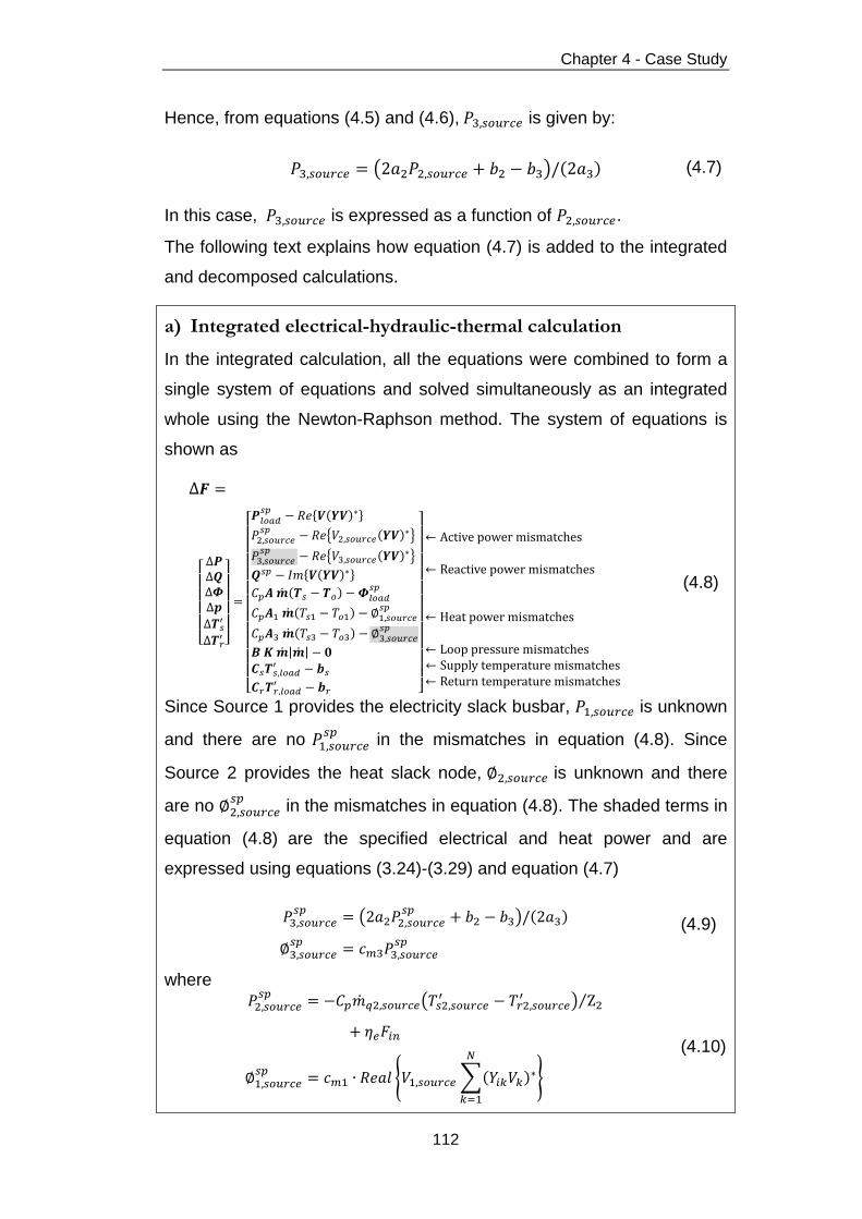
Chapter 4 - Case Study
112
Hence, from equations (4.5) and (4.6), is given by:
(4.7)
In this case, is expressed as a function of .
The following text explains how equation (4.7) is added to the integrated
and decomposed calculations.
a) Integrated electrical-hydraulic-thermal calculation
In the integrated calculation, all the equations were combined to form a
single system of equations and solved simultaneously as an integrated
whole using the Newton-Raphson method. The system of equations is
shown as
(4.8)
Since Source 1 provides the electricity slack busbar, is unknown
and there are no
in the mismatches in equation (4.8). Since
Source 2 provides the heat slack node, is unknown and there
are no
in the mismatches in equation (4.8). The shaded terms in
equation (4.8) are the specified electrical and heat power and are
expressed using equations (3.24)-(3.29) and equation (4.7)
(4.9)
where
(4.10)

Chapter 4 - Case Study
113
This means the electrical power of Source 2 and Source 3 are expressed
as functions of the variables of the heat network. The heat power of
Source 1 is expressed as a function of the variables of the electricity
network. Therefore, comparing to Chapter 3, the elements
in the
electricity to heat Jacobian submatrix are nonzero.
b) Decomposed electrical-hydraulic-thermal calculation
The flowchart of the decomposed electrical-hydraulic-thermal calculation
is illustrated through the linkages shown in Figure 4.11. The linkages are
formed by three sources with unknown heat and electrical power.
Φ1,source, Φ3,source
Φ2,source
(heat slack)
Hydraulic and thermal
calculation
P2,source
Z2
P1,source
(electricity slack)
Electrical power flow
calculation
Φ1,source
P3,source
Equation (4.7)
Φ3,source
cm3
cm1
Output results
Max(|ΔΦ1,source,Φ3,source|)<ε?
Yes
Input data
Figure 4.11: Flowchart of the decomposed electrical-hydraulic-thermal calculation

Chapter 4 - Case Study
114
If the result of the electrical power generation of a source exceeds its
generation upper or lower limit, then the lower or upper limit is the
electrical power output from the source. For other sources, the same
calculation process described in this section is performed again.
The cases with N (N ≥ 3) sources can be similarly implemented as that of
. The equal-incremental-fuel-cost criterion is then applied to the
electrical power of N-1 sources.
It is assumed that in equation (4.4)
[8]. By substituting
these values in equations (4.4) – (4.7):
(4.11)
(4.12)
(4.13)
The initial values were the same as those of the Barry Island case study
in Section 4.3. In addition, initially assume
.
Using the integrated electrical-hydraulic-thermal calculation technique,
the model equations were solved in 15 iterations with the tolerance ε =
10-3. Using the decomposed electrical-hydraulic-thermal calculation, the
model equations were solved in 43 iterations with the tolerance ε = 10-3.
The results of the integrated and decomposed calculations were very
close at 10-3 precision.

Chapter 4 - Case Study
115
The results of the calculation of the heat and electrical power from
Source 1, Source 2 and Source 3 are shown in Figure 4.12. The
incremental fuel cost is 12.60£/MWh. The total cost of Source 1,
Source 2 and Source 3 for supplying electricity over an hour is:
. Substituting the
power flow results shown in Figure 4.5 into equation (4.11) of the cost
function, the total cost is calculated as 170.60£/h. Comparing the two
results, the results of optimal dispatch save 0.38£/h.
Figure 4.12: Heat and electrical power supplied from three sources
4.7 Summary
This chapter provided an engineering solution to the Barry Island case
study. The case study examined how both electrical and heat demands
in a self-sufficient system (no interconnection with external systems)
were met using CHP units.
The combined analysis took into account the flows of energy between
the electricity and heat networks through the CHP units. The combined
analysis in the forms of the power flow and optimal dispatch was solved
by the Newton-Raphson method. The variables of the electrical and heat
networks were calculated. These included: heat and electrical power of
0.3632 0.4721
0.4983
0.8239
0.7496
0.9488 1.6
2.164
0
0.5
1
1.5
2
2.5
0
0.5
1
1.5
2
2.5
Electricity Heat
Source 3
Source 2
Source 1
Load

Chapter 4 - Case Study
116
the CHP units, mass flow rates, supply and return temperatures, voltage
magnitudes and voltage angles, heat and electrical power losses.
The combined analysis consisted of the decomposed and integrated
calculation techniques. The comparison showed that the integrated
calculation requires fewer iterations than the decomposed calculation.

Chapter 5 - Conclusions
5.1 Conclusions
The use of CHP units, heat pumps and electric boilers increases the
linkages between electricity and heat networks. A combined analysis
was developed to investigate the performance of electricity and heat
networks as an integrated whole. This was based on a model of
electrical power flow and hydraulic and thermal circuits together with
their coupling components (CHP units, heat pumps, electric boilers and
circulation pumps). The flows of energy between the electricity and heat
networks through the coupling components were taken into account.
The combined analysis was used for the delivery of the electrical and
heat energy from CHP units and heat pumps and other coupling
components to the consumers through electrical and heat networks. It
consisted of the decomposed and integrated electrical-hydraulic-thermal
calculation techniques in the forms of the power flow and simple optimal
dispatch. The integrated calculation required fewer iterations and the
number of the iterations of the decomposed calculation increases with
the size of the networks.
5.1.1 Analysis of District Heating Networks
Hydraulic-thermal model was developed to investigate the performance
of a district heating network. The objective of the hydraulic-thermal
model was to determine the mass flow rates within each pipe and the
Chapter 5 - Conclusions
118
load supply temperatures and the source return temperatures. It was
assumed that the source supply temperatures and the load return
temperatures were specified; the injected mass flow rates or the heat
power supplied or consumed at all the nodes except one were specified.
The individual hydraulic and thermal models in district heating networks
were modelled. In the hydraulic model, the network description was
based on a graph-theoretical method. Two calculation methods were
investigated for the hydraulic calculation of looped networks. The
Newton-Raphson method considered all loops simultaneously. The
Hardy-Cross method dealt with one loop at a time. The adjustments of
the Hardy-Cross method used the main diagonal of the Jacobian matrix
of the Newton-Raphson method. For the sake of combining with the
thermal model and further combining with the electrical power flow, the
Newton-Raphson method was used to solve the hydraulic equations. In
the thermal model, the mixture temperatures at nodes were considered,
and a matrix formulation of the thermal model was implemented.
Conventionally, the decomposed hydraulic-thermal calculation was
through an iterative procedure between the individual hydraulic and
thermal models. In this thesis, an integrated hydraulic-thermal calculation
was developed, in which the hydraulic and thermal models were
combined in a single system of equations solved by the Newton-
Raphson method. It took into account the coupling between the
individual hydraulic and thermal analyses. For instance, the thermal
calculation cannot be performed without knowing the pipe mass flows,
and the hydraulic calculation cannot be performed without knowing
temperatures under the assumption that the nodal heat power is
specified.
The results of the decomposed and integrated hydraulic-thermal
calculations were very close to 10-3 precision. The results were validated
using SINCAL with the same value at 10-3 precision.

Chapter 5 - Conclusions
119
5.1.2 Combined Analysis of Electricity and Heat Networks
Two calculation techniques (decomposed and integrated electrical-
hydraulic-thermal calculations) were developed. Three combinations of
coupling mechanisms (CHP only; CHP and circulation pump; CHP,
circulation pump and heat pump) were considered in each calculation
technique. The calculation techniques were demonstrated in the grid-
connected and the islanded operation modes.
In the grid-connected mode, any surplus or deficit in electrical power is
supplied from the main grid and not from the CHP units, thus there is no
linkage back from the electrical system to the heat system. While in the
islanded mode there are bidirectional linkages between the electricity
and heat networks.
For the decomposed electrical-hydraulic-thermal calculation in the grid-
connected mode, the hydraulic-thermal model was solved first. Then
these results were transferred to the electricity network through the
coupling components. Finally the electrical power flow model was solved.
In the islanded mode, this sequential procedure was iterated until the
solution converged within an acceptable tolerance.
For the integrated electrical-hydraulic-thermal calculation, the electrical
power flow equations, the hydraulic equations and the thermal equations
were combined to form a single system of equations and solved
simultaneously as an integrated whole using the Newton-Raphson
method.
The combined analysis has the ability to calculate the variables of the
electrical and heat networks, which can be used for the design and
operation of integrated heat and electricity systems. These variables
included: heat and electrical power from the CHP units, mass flow rates,
supply and return temperatures, voltage magnitudes and voltage angles,
heat and electrical power losses. This was based on the assumptions
that the source supply temperatures and the load return temperatures
were specified; the injected nodal heat and electrical power supplied or
Chapter 5 - Conclusions
120
consumed at non-slack nodes or busbars were specified; and the voltage
magnitudes at source busbars were specified.
The results of the decomposed and integrated electrical-hydraulic-
thermal calculations were very close to 10-3 precision. The real values
were used in the calculation of heat networks and the per unit was used
in the calculation of electrical networks. The convergence characteristics
of two calculations were compared. The comparison showed that the
integrated calculation requires fewer iterations than the decomposed
calculation. In a simple example network, the decomposed calculation
was solved in 16 iterations and the integrated calculation was solved in
12 iterations.
5.1.3 Case Study
A case study of Barry Island was conducted. The heat network was a low
temperature looped pipe district heating network with 32 nodes and fed
by three CHP units. The electrical power from three CHP units was
supplied to 5 lumped electrical loads. The case study examined how
both electrical and heat demands in a self-sufficient system (no
interconnection with external systems) were met using CHP units. To
benefit from the efficient heat and electricity generation of CHP units, a
solution was demonstrated to deliver the electrical and heat energy from
the CHP units to the consumers through electrical and heat networks.
In this case study, the combined analysis consisted of the forms of the
power flow and simple optimal dispatch. In the power flow, the
decomposed calculation was solved in 33 iterations and the integrated
calculation was solved in 14 iterations. In optimal dispatch, the
decomposed calculation was solved in 43 iterations and the integrated
calculation was solved in 15 iterations. Comparing to the simple example
network, it can be seen that the integrated calculation requires fewer
iterations and the number of the iterations of the decomposed calculation
increases with the size of the networks.
The results of the decomposed and integrated electrical-hydraulic-
thermal calculations were very close to 10-3 precision. The results of heat

Chapter 5 - Conclusions
121
variables were validated using SINCAL and the results of electrical
variables were validated using IPSA. The comparison showed these
results were very close to 10-3 precision.
The combined analysis can be used for the design and operation of
integrated heat and electricity systems for energy supply to buildings.
This will increase the flexibility of the electricity and heat supply systems
for facilitating the integration of intermittent renewable energy.
5.2 Contributions of the Thesis
Contributions of the thesis are as follows:
· For the analysis of district heating networks, a power flow formulation
analogous to the electrical power flow was described. Decomposed
and integrated hydraulic-thermal calculation techniques were
developed. In the integrated method, the Newton-Raphson method
was employed to solve the hydraulic-thermal model.
· The coupling components model: three types of CHP units and a
CHP and heat pump composite supply system were modelled. This
provides linkages between electricity and heat networks.
· Two combined analysis methods were developed to investigate the
performance of electricity and heat networks as an integrated whole.
These two methods were the decomposed and integrated electrical-
hydraulic-thermal calculation techniques in the forms of the power
flow and simple optimal dispatch.
· The formulation of the integrated method reduces dimensionality. The
comparison showed that the integrated method requires fewer
iterations than the decomposed method.
· The models focused on network analysis. Variables (voltage, mass
flow rates, temperature, electricity losses and heat losses) were
calculated precisely for a network with arbitrary topology.

Chapter 5 - Conclusions
122
· An engineering solution was provided to the Barry Island case study.
5.3 Future Work
Recommendations for further work are as follows:
1) Applications of the combined analysis
· The impacts of the different penetration of CHP units and heat pumps
on the electricity and heat networks may be investigated. For
example, the generation capacity of the CHP units may range
0~100% of the total electricity supply.
· The impact of heat networks on electricity distribution networks and
vice versa may be investigated. For example, the variations of heat
demand to the operation of electrical networks.
· A consideration of local decentralised generation may be of interest,
such as local heat pumps or electric boilers installed at consumers
and interconnected to heat networks.
· An extension of optimal dispatch may be required. The fuel cost may
be modelled as a function of both electrical and heat power.
2) Further development of the combined analysis
· The inclusion of thermal storage in a multi-time simulation may be
conducted.
· The integration of more energy vectors may be considered, e.g., gas,
cooling.
· An extension of the model to optimal power flow may be developed.
The most energy efficient operating regime will be determined and
energy losses, costs or gaseous emissions minimised.

Reference
[1] Department of Energy & Climate Change, "2011 UK greenhouse gas emissions: Final figures," 2013.
[2] Office of Public Sector Information, "Climate Change Act 2008," 2008. [3] A. Simpson, "Briefing: Renewable Heat Incentive," Friends of the Earth,
2010. [4] H. Lund, A. N. Andersen, P. A. Østergaard, B. V. Mathiesen, and D.
Connolly, "From electricity smart grids to smart energy systems – A market operation based approach and understanding," Energy, vol. 42, pp. 96-102, 2012.
[5] Department of Energy and Climate Change, The future of heating: Meeting the challenge, March 2013.
[6] R. Platt, W. Cook, and A. Pendleton, "Green Streets, Strong Communities," Institute for Public Policy Research, 2011.
[7] M. Geidl and G. Andersson, "Optimal Power Flow of Multiple Energy Carriers," Power Systems, IEEE Transactions on, vol. 22, pp. 145-155, 2007.
[8] B. M. Weedy, B. J. Cory, N. Jenkins, J. B. Ekanayake, and G. Strbac, Electric power systems 5th ed.: Wiley, 2012.
[9] G. Harrison and R. Wallace, "Network integration of CHP: how to maximize access," Cogeneration and On-Site Power Production, vol. 5, pp. 69-76, 2004.
[10] CHPA, "Integrated Energy: The role of CHP and district heating in our energy future," The Combined Heat and Power Association (CHPA), 2010.
[11] H. Zhao, "Analysis, modelling and operational optimization of district heating systems," PhD Thesis, Technical University of Denmark, 1995.
[12] G. Davies and P. Woods, "The Potential and Costs of District Heating Networks," 2009.
[13] J. Kunz, P. Haldi, and G. Sarlos, "Dynamic behavior of district heating systems," Begell House Publishers, 1994.
[14] B. Skagestad and P. Mildenstein, "District Heating and Cooling Connection Handbook," International Energy Agency, IEA.
[15] P. Johansson, "Buildings and District Heating - Contributions to Development and Assessments of Efficient Technology," PhD thesis, Dept. of Energy Sciences, Faculty of Engineering, Lund University, 2011.
[16] Heat and the City. Available: http://www.heatandthecity.org.uk/ [Accessed: 07.03.2013]
[17] CHPA, "The role of CHP and district heating in our energy future," ed: The Combined Heat and Power Association (CHPA), 2010.
[18] G. Strbac, N. Jenkins, and T. Green, "Future network technologies," Report to DTI, 2006.
[19] CIBSE, "Guide to Community Heating and CHP (Good practice guide (GPG) 234) " the Chartered Institution of building services engineer (CIBSE).
[20] BERR, "Heat Call for Evidence," Deparment for Business Enterprise & Regulatory Reform, Jan 2008.
[21] Department of Energy & Climate Change, Strategic Framework for Low Carbon Heat in the UK: Summary of Responses, 2012.

Reference
124
[22] HM Government, "The Carbon Plan: Delivering our low carbon future," 2011.
[23] R. Wiltshire, "The UK potential for community heating with combined heat and power," Building Research Establishment. Watford, UK, BRE, 2003.
[24] F.Starr, "Future Challenges for CHP in the UK and Continental Europe," Claverton2010.
[25] S. Kelly and M. G. Pollitt, "Making Combined Heat and Power District Heating (CHP-DH) networks in the United Kingdom economically viable: a comparative approach," University of Cambridge, Faculty of Economics, 2009.
[26] N. Jenkins, G. Strbac, and J. Ekanayake, Distributed Generation: The Institution of Engineering and Technology, 2010.
[27] P. Woods. (2012). The Case for District Heating – a flexible energy system. Available: http://cardiff.ac.uk/ugc/flexible-energy-delivery-system-seminar-series-for-postgraduates-and-researchers [Accessed: 05.10.2012]
[28] LCICG, Technology Innovation Needs Assessment (TINA) Heat Summary Report: Low Carbon Innovation Coordination Group, September 2012.
[29] P. Woods, "Comparing CHP/DH with other technologies," CIBSE Seminar, 2011.
[30] Department of Energy & Climate Change, "Heat and Energy Saving Strategy Consultation " 2009.
[31] DECC and DCLG, " Warm Homes, Greener Homes: A Strategy for Household Energy Management Supporting Paper VIII, An Enabling Framework for District Heating and Cooling," Department of Energy & Climate Change, 2010.
[32] Postnote, "Renewable Heating," The Parliamentary Office of Science and Technology, 2010.
[33] Committee on Climate Change, "The Fourth Carbon Budget - Reducing emissions through the 2020s," 2010.
[34] A. Molyneaux, G. Leyland, and D. Favrat, "Environomic multi-objective optimisation of a district heating network considering centralized and decentralized heat pumps," Energy, vol. 35, pp. 751-758, 2010.
[35] CHP Focus. Available: http://chp.decc.gov.uk/cms/ [36] IEA, "Technology Roadmap Energy-efficient Buildings: Heating and
Cooling Equipment," International Energy Agency, 2011. [37] DESIRE. Dissemination Strategy on Electricity Balancing for Large
Scale Integration of Renewable Energy Available: http://desire.iwes.fraunhofer.de/home.htm [Accessed: 21.06.2011]
[38] W. C. Turkenburg, D. J. Arent, R. Bertani, A. Faaij, M. Hand, W. Krewitt, E. D. Larson, J. Lund, M. Mehos, T. Merrigan, C. Mitchell, J. R. Moreira, W. Sinke, V. Sonntag-O’Brien, B. Thresher, W. van Sark, E. Usher, and E. Usher, "Chapter 11 - Renewable Energy," in Global Energy Assessment - Toward a Sustainable Future, ed Cambridge University Press, Cambridge, UK and New York, NY, USA and the International Institute for Applied Systems Analysis, Laxenburg, Austria, 2012, pp. 761-900.
[39] E.ON starts construction of power-to-gas pilot plant in Germany. Available: http://www.eon.com/en/media/news/press-releases/2012/8/21/eon-startsconstruction-of-power-to-gas-pilot-plant-in-germany.html?fromSearchResult=true [Accessed: 07.11.2012]
Reference
125
[40] E.ON launches project unique in Europe to store heat from renewable energy sources. Available: http://www.eon.com/en/media/news/press-releases/2011/7/1/e-dot-on-launches-project-unique-in-europe-to-store-heat-from-renewable-energy-sources.html?fromSearchResult=true [Accessed: 07.11.2012]
[41] M. Geidl, "Integrated modeling and optimization of multi-carrier energy systems," PhD Thesis, the Swiss Federal Institute of Technology (ETH), 2007.
[42] P. Mancarella, "Smart Multi-Energy Grids: Concepts, Benefits and Challenges " IEEE PES General Meeting 2012, 2012.
[43] G. Chicco and P. Mancarella, "Distributed multi-generation: A comprehensive view," Renewable and Sustainable Energy Reviews, vol. 13, pp. 535-551, 2009.
[44] P. Mancarella, "MES (multi-energy systems): An overview of concepts and evaluation models," Energy, vol. 65, pp. 1-17, 2014.
[45] P. Mancarella and G. Chicco, "Distributed Multi-Generation: energy models and analyses": Nova Publisher, New York, 2009.
[46] R. Knight. (2012). Smart Systems in the UK context – an ETI view. Available: http://eti.co.uk/downloads/related_documents/Smart_Cities_Richard_Knight_17th_April_2012.pdf [Accessed: 20.09.2012]
[47] F. Kienzle, P. Favre-Perrod, M. Arnold, and G. Andersson, "Multi-energy delivery infrastructures for the future," in Infrastructure Systems and Services: Building Networks for a Brighter Future (INFRA), 2008 First International Conference on, 2008, pp. 1-5.
[48] P. Mancarella, "Multi-energy Systems: The Smart Grid beyond Electricity," LBL, Berkeley, 2012.
[49] P. Mancarella, "Distributed Multi-Generation Options to Increase Environmental Efficiency in Smart Cities " IEEE PES General Meeting 2012, 2012.
[50] A. Seungwon, L. Qing, and T. W. Gedra, "Natural gas and electricity optimal power flow," Transmission and Distribution Conference and Exposition, IEEE PES, vol. 1, pp. 138-143, 2003.
[51] M. Chaudry, N. Jenkins, and G. Strbac, "Multi-time period combined gas and electricity network optimisation," Electric Power Systems Research, vol. 78, pp. 1265-1279, 2008.
[52] M. Qadrdan, M. Chaudry, J. Wu, N. Jenkins, and J. Ekanayake, "Impact of a large penetration of wind generation on the GB gas network," Energy Policy, vol. 38, pp. 5684-5695, 2010.
[53] A. Martinez-Mares and C. R. Fuerte-Esquivel, "A Unified Gas and Power Flow Analysis in Natural Gas and Electricity Coupled Networks," Power Systems, IEEE Transactions on, vol. 27, pp. 2156-2166, 2012.
[54] R. Rubio-Barros, D. Ojeda-Esteybar, and A. Vargas, "Energy Carrier Networks: Interactions and Integrated Operational Planning Handbook of Networks in Power Systems II," A. Sorokin, S. Rebennack, P. M. Pardalos, N. A. Iliadis, and M. V. F. Pereira, Eds., ed: Springer Berlin Heidelberg, 2012, pp. 117-167.
[55] P. Favre-Perrod, "Hybrid energy transmission for multi-energy networks," PhD Thesis, ETH, 2008.
[56] B. Awad, M. Chaudry, J. Wu, and N. Jenkins, "Integrated optimal power flow for electric power and heat in a microgrid," Prague, 2009.
[57] M. T. Rees, J. Wu, B. Awad, J. Ekanayake, and N. Jenkins, "A modular approach to integrated energy distribution system analysis," 17th Power Systems Computation Conference, Stockholm Sweden, 2011.

Reference
126
[58] M. T. Rees, J. Wu, B. Awad, J. Ekanayake, and N. Jenkins, "A total energy approach to integrated community infrastructure design," Power and Energy Society General Meeting, 2011 IEEE, 2011.
[59] H. Lund and E. Münster, "Integrated energy systems and local energy markets," Energy Policy, vol. 34, pp. 1152-1160, 2006.
[60] P. Meibom, J. Kiviluoma, R. Barth, H. Brand, C. Weber, and H. V. Larsen, "Value of electric heat boilers and heat pumps for wind power integration," Wind Energy, vol. 10, pp. 321-337, 2007.
[61] G. Chicco and P. Mancarella, "Evaluation of multi-generation alternatives: an approach based on load transformations," in Power and Energy Society General Meeting - Conversion and Delivery of Electrical Energy in the 21st Century, 2008 IEEE, 2008, pp. 1-6.
[62] M. Pierluigi, "Cogeneration systems with electric heat pumps: Energy-shifting properties and equivalent plant modelling," Energy Conversion and Management, vol. 50, pp. 1991-1999, 2009.
[63] R. Sansom, "The impact of future heat demand pathways on the economics of low carbon heating systems," BIEE Conference, 2012.
[64] J. Arran and J. Slowe, "2050 Pathways for Domestic Heat Final Report " Delta Energy & Environment Ltd, 2012.
[65] J. Speirs, R. Gross, S. Deshmukh, P. Heptonstall, L. Munuera, M. Leach, and J. Torriti, "Heat delivery in a low carbon economy," BIEE Conference, 2010.
[66] P. Dodd, "Delivering the low carbon energy jigsaw. Will the technology and incentive pieces fit," 2012.
[67] Siemens, "PSS Sincal 7.0 heating Manual," 2010. [68] M. Fedorov, "Parallel Implementation of a Steady State Thermal and
Hydraulic Analysis of Pipe Networks in OpenMP," in Parallel Processing and Applied Mathematics. vol. 6068, R. Wyrzykowski, J. Dongarra, K. Karczewski, and J. Wasniewski, Eds., ed: Springer Berlin / Heidelberg, 2010, pp. 360-369.
[69] B. E. Larock, R. W. Jeppson, and G. Z. Watters, Hydraulics of pipeline systems: CRC, 2000.
[70] A. Osiadacz, Simulation and analysis of gas networks: Gulf Pub. Co., 1987.
[71] 7-Technologies, "TERMIS Help Manual," 2009. [72] A. Benonysson, "Dynamic Modelling and Operational Optimization of
District Heating Systems," PhD Thesis. Laboratory of Heating and Air Conditioning. Technical University of Denmark, 1991.
[73] I. Ben Hassine and U. Eicker, "Impact of load structure variation and solar thermal energy integration on an existing district heating network," Applied Thermal Engineering, 2012.
[74] G. P. Henze and A. G. Floss, "Evaluation of temperature degradation in hydraulic flow networks," Energy and Buildings, vol. 43, pp. 1820-1828, 2011.
[75] D. Clamond, "Efficient resolution of the Colebrook equation," Industrial & Engineering Chemistry Research, vol. 48, pp. 3665-3671, 2009.
[76] W. H. Press, S. A. Teukolsky, W. T. Vetterling, and B. P. Flannery, "Numerical Recipes 3rd Edition: The Art of Scientific Computing " Cambridge University Press, 2007.
[77] MathWorld. Newton's Method. Available: http://mathworld.wolfram.com/NewtonsMethod.html [Accessed: 01.05.2010]
Reference
127
[78] T. Altman and P. F. Boulos, "Convergence of Newton method in nonlinear network analysis," Mathematical and Computer Modelling, vol. 21, pp. 35-41, 1995.
[79] K. C. B. Steer, A. Wirth, and S. K. Halgamuge, "Control period selection for improved operating performance in district heating networks," Energy and Buildings, vol. 43, pp. 605-613, 2011.
[80] J. Byun, Y. Choi, J. Shin, M. Park, and D. Kwak, "Study on the Development of an Optimal Heat Supply Control Algorithm for Group Energy Apartment Buildings According to the Variation of Outdoor Air Temperature," Energies, vol. 5, pp. 1686-1704, 2012.
[81] B. Bøhm and P. O. Danig, "Monitoring the energy consumption in a district heated apartment building in Copenhagen, with specific interest in the thermodynamic performance," Energy and Buildings, vol. 36, pp. 229-236, 2004.
[82] L. Saarinen, "Modelling and control of a district heating system," Uppsala University, Department of Information Technology, p. 12, 2008.
[83] B. Bøhm, S. Ha, W. Kim, B. Kim, T. Koljonen, H. Larsen, M. Lucht, Y. Park, K. Sipila, and M. Wigbels, Simple models for operational optimisation: Department of Mechanical Engineering, Technical University of Denmark, 2002.
[84] J. M. Coulson, J. F. Richardson, and R. K. Sinnott, "Coulson & Richardson’s Chemical Engineering. Volume 1: Fluid Flow, Heat Transfer & Mass Transfer," Butterworth-Heinemann Ltd, p. 501, 1999.
[85] J. McCalley. Power System Analysis I (Fall 2006) Course. Available: www.ee.iastate.edu/~jdm/EE456/FastPowerFlow.doc [Accessed: 08.11.2012]
[86] J. J. Grainger and W. D. Stevenson, Power system analysis: McGraw-Hill (New York), 1994.
[87] J. Kalina and J. Skorek, "CHP plants for distributed generation–equipment sizing and system performance evaluation," Proceeding of ECOS, 2002.
[88] C. Sondergren and H. F. Ravn, "A method to perform probabilistic production simulation involving combined heat and power units," Power Systems, IEEE Transactions on, vol. 11, pp. 1031-1036, 1996.
[89] L. Goldstein, Gas-fired distributed energy resource technology characterizations: National Renewable Energy Laboratory, 2003.
[90] EPA, Catalog of CHP Technologies: U.S. Environmental Protection Agency (EPA) Combined Heat and Power Partnership, 2008.
[91] EURELECTRIC, "European Combined Heat & Power: A Technical Analysis of Possible Definition of the Concept of “Quality CHP”," Union of the Electricity Industry – EURELECTRIC, 2002.
[92] H. Palsson, "Methods for planning and operating decentralized combined heat and power plants," Technical University of Denmark, 2000.
[93] H. V. Larsen, H. Pálsson, and H. F. Ravn, "Probabilistic production simulation including combined heat and power plants," Electric Power Systems Research, vol. 48, pp. 45-56, 1998.
[94] CHPQA. GUIDANCE NOTE 28: The Determination of Z Ratio. Available: https://www.chpqa.com/guidance_notes/GUIDANCE_NOTE_28.pdf [Accessed: 01.06.2013]
[95] Danfoss. The Heating Book - 8 steps to control of heating systems. Available: http://heating.danfoss.com/Content/61078BB5-1E17-4CA2-

Reference
128
AC49-8A7CAC2BA687_MNU17424997_SIT54.html [Accessed: 23.07.2012]
[96] A. Seugwon, "Natural Gas and Electricity Optimal Power Flow," PhD thesis, Oklahoma State University, 2004.
[97] MATPOWER. Available: http://www.pserc.cornell.edu/matpower/ [Accessed: 03.04.2010]
[98] Y. Xing, A. Bagdanavicius, S. C. Lannon, M. Pirouti, and T. Bassett, "Low temperature district heating network planning with the focus on distribution energy losses," The Fourth International Conference on Applied Energy (ICAE2012), Suzhou, China, 2012.
[99] S. Ingram, S. Probert, and K. Jackson, "The Impact of Small Scale Embedded Generation Upon The Operating Parameters of Distribution Networks," DTi New and Renewable Energy Program, K/EL/00303/04/01, 2003.
[100] IPSA Power Available: http://www.ipsa-power.com/ [Accessed: 03.04.2013]
[101] T. Guo, M. I. Henwood, and M. van Ooijen, "An algorithm for combined heat and power economic dispatch," Power Systems, IEEE Transactions on, vol. 11, pp. 1778-1784, 1996.
[102] J. D. Glover, M. S. Sarma, and T. J. Overbye, Power Systems Analysis & Design: Thomson, 2008.

Appendix A - Hydraulic Calculation
Methods
The objective of the hydraulic model is to determine the pipe mass flow
rates under the assumption that the nodal mass flow rates are
specified. The set of the hydraulic equations was written in the forms of
unknown pipe mass flow rates , unknown pressure head h, or unknown
corrective mass flow rates . The -equations solved by the Newton-
Raphson method was described in Chapter 2. In this Appendix, the h-
equations solved by the Newton-Raphson and the -equations solved
by the Newton-Raphson and the Hardy-Cross method were explained by
a simple example and a more complicated example.
A1 A Simple Example
A simple example of a pipe network with a loop is shown in Figure A.1.
1
4kg/s 1kg/s
2 3m2.
m3.
m1.
mq2 mq3
1
. .
21 3
5kg/s
mq1.
Figure A.1: A pipe network with a loop
For the pipe network, the nodal mass flow rates are
.
It was assumed that the vector of the resistance coefficients of each pipe
K is constant and is given by, .

Appendix A - Hydraulic Calculation Methods
130
The network incidence matrix A and the loop incidence matrix B are:
A =
B =
a) -equations
The continuity equation for nodes 1 and 2 is
(A.1)
The loop pressure equation for loop 1 is
(A.2)
b) h-equations
The mass flow rate is written in the form of the pressure head using
equation (2.9)
(A.3)
where is the mass flow rate in pipe k between nodes i and j.
By substituting in equation (A.1):
(A.4)
c) -equations
1 2 3
1 1 -1 1
Loop N
o.
Pipe No. 1 2 3
1 1 -1 0
2 0 1 1
3 -1 0 -1
Node N
o.
Pipe No.

Appendix A - Hydraulic Calculation Methods
131
Choose initial values of in each pipe, such that the continuity
equation (A.1) is satisfied (e.g.,
). The mass flow rate
in each pipe is replaced by an initial flow rate, denoted by , plus the
unknown corrective flow rate that circulates through each pipe.
(A.5)
Three systems of equations were described:
· Equations (2.27) and (2.28) with unknown variables
· Equation (A.4) with unknown variables
· Equation (A.5) with unknown variable
The number of -equations is equal to the number of pipes. The number
of h-equations is equal to the number of nodes minus one. The number
of -equations is equal to the number of loops.
A2 Solutions
The Newton-Raphson method for solving -equations has been
described in the hydraulic model in Chapter 2.
A2.1 h-equations using the Hardy-Cross method
The h-equations is solved using the Newton-Raphson method.
The iterative form of the Newton-Raphson method is
(A.6)
where is the pressure head mismatches.

Appendix A - Hydraulic Calculation Methods
132
The Jacobian matrix is formed similarly as the admittance matrix in
electric power system. The Jacobian matrix for equation (A.4) is
(A.7)
Assuming the pressure head at node 3 is the reference head h3 = 10Pa,
and the initial heads at nodes 1 and 2 are: h1 = 20Pa, h2 = 4Pa. For the
first iteration,
.
After 4251 iterations with the tolerance ε = 10-3, the converged results
are h = [21.9988 3.9976 10.0000]T. By substituting h in equation (A.3),
the calculated mass flow rates are = [1.9998 3.0002 1.0005]T.
It was found that the h-equations with the nodal formulation encountered
convergence difficulty in the case of improper selection of initial nodal
head values.
A2.2 -equations using the Newton-Raphson method
The unknown variables are the corrective mass flow rates in each pipe in
-equations. The initial value of the mass flow rate in each pipe is
chosen such that the continuity equation is satisfied. By changing the
mass flow rates in all the pipes in loop li by the same amount , the
increase or decrease in the flow into a junction is balanced by the exact
same increase or decrease in the flow out, so that the continuity equation
is still satisfied.
The mass flow rates within each pipe is calculated from the corrective
mass flow rates in each loop
(A.8)
where is the nl × 1 vector, nl is the number of loops.
The iterative form of the Newton-Raphson method is
(A.9)
The Jacobian matrix is

Appendix A - Hydraulic Calculation Methods
133
(A.10)
The loop pressure mismatches are
(A.11)
The derivative of to (
) is
(A.12)
For the network as shown in Figure A.1, the Jacobian matrix J is
(A.13)
Initially assume .
For the first iteration,
.
After 4 iterations with the tolerance ε = 10-3, the converged results are:
.
Thus, from equation (A.8),
.
A2.3 -equations using the Hardy-Cross method
Hardy-Cross method was developed for hand calculations and solved
one loop at a time instead of solving all loops simultaneously. The
iterative form is

Appendix A - Hydraulic Calculation Methods
134
(A.14)
The adjustments use the main diagonal of Jacobain matrix in the
Newton-Raphson method. The adjustments of the pipe flow rates in all
loops are
(A.15)
where, np and nl are the number of pipes and loops; k is the index of
loops; |B| consists of elements ‘1’ and ‘0’. For a pipe in two loops, the
adjustments of its flow rate are cumulative. The procedure to calculate
is explained in the Newton-Raphson method.
Comparing to the Newton-Raphson method in the -equations, the
Hardy Cross method simplifies the determination of the correction term
by considering each loop independently rather than all loops
simultaneously.
The steps of the hydraulic calculation for the network as shown in Figure
A.1 are as follows:
1) Choose initial values of in each pipe, such that the continuity
equation is satisfied (e.g.,
).
2) Calculate the sum of head loss around the loop using equation (A.5).
For the first iteration,
.
3) Calculate the derivative of the expression in step 2. For the first
iteration,
.

Appendix A - Hydraulic Calculation Methods
135
4) Adjust the mass flow rates within each pipe in the loop by the same
amount . This adjustment is calculated by dividing the result from
step 2 by the result from step 3. For the first iteration,
. Thus,
.
5) This procedure is repeated from step 2) until the maximum of
becomes less than ε. After 4 iterations, the converged results are:
.
A3 A Complicated Example
Another case represents a part of a district heating network with multi-
loops is shown in Figure A.2. The network is supplied by node 1. The
pipe parameters, nodal mass flow vector , the network incidence
matrix A and the loop incidence matrix B are listed in Table A.1-A.4.
1
9
8 13
2
7 6
10 1211
43 51 2
4
5
6
7
8
9
10
11
12
13
14
16
15
3
1 2
43
Figure A.2: A district heating network with multi-loops

Appendix A - Hydraulic Calculation Methods
136
Table A.1: Pipe parameters
Pipe No. Node No.
(start)
Node No.
(end)
Diameter
(m)
Length
(m)
Roughness
(mm)
1 1 2 0.25 200 0.025
2 2 3 0.20 80 0.025
3 1 7 0.05 352 0.025
4 3 7 0.05 112 0.025
5 3 4 0.20 240 0.025
6 4 6 0.05 328 0.025
7 4 5 0.15 96 0.025
8 5 6 0.125 248 0.025
9 1 8 0.08 160 0.025
10 8 9 0.05 104 0.025
11 9 10 0.05 208 0.025
12 10 13 0.15 200 0.025
13 2 13 0.30 48 0.025
14 10 11 0.10 120 0.025
15 11 12 0.08 208 0.025
16 4 12 0.10 280 0.025
Table A.2: Mass flow rate at each node
Node 1 2 3 4 5 6 7 8 9 10 11 12
129.37 2.96 4.37 7.38 9.16 27.03 1.96 4.65 5.85 28.29 26.67 7.68
Table A.3: Data of the network incidence matrix A
Pipe No.
1 2 3 4 5 6 7 8 9 10 11 12 13 14 15 16
No
de
No
.
1 -1 -1 -1
2 1 -1 -1
3 1 -1 -1
4 1 -1 -1 -1
5 1 -1
6 1 1
7 1 1
8 1 -1
9 1 -1
10 1 -1 -1
11 1 -1
12 1 1

Appendix A - Hydraulic Calculation Methods
137
Table A.4: Data of the loop incidence matrix B
Pipe No.
1 2 3 4 5 6 7 8 9 10 11 12 13 14 15 16
Lo
op
No
.
1 -1 1 1 1 1 -1
2 -1 -1 -1 1 1 1 -1
3 1 1 -1 1
4 -1 1 1
A3.1 -equations using the Newton-Raphson method
For the network as shown in Figure A.2, the Jacobian matrix J is
(A.16)
where
,
,
,
.
After 6 iterations with the tolerance ε=10-3, the converged results are:
= [119.06 62.13 1.47 0.49 57.28 2.14 34.05 24.89 8.83 4.18 -1.67 -
50.60 53.97 20.64 -6.03 13.71].
A3.2 -equations using the Hardy-Cross method
The steps of the hydraulic calculation for the network with 4 loops as
shown in Figure A.2 are as follows
1) Choose initial values of in each pipe to satisfy the continuity
equation:
· Arbitrarily choose values for one pipe in each loop to form 4
augmented equations, for example, pipe 11 in loop 1, pipe 16 in

Appendix A - Hydraulic Calculation Methods
138
loop 2, pipe 3 in loop 3, pipe 6 in loop 4, e.g., set their values to 1
kg/s.
· Combine these augmented equations and the continuity equations
to calculate the initial mass flow rates
= [116.87 49.90 1.00 0.96 44.57 1.00 35.19 26.03 11.50 6.85
1.00 -60.64 64.01 33.35 6.68 1.00]T.
2) Calculate the sum of head loss around each loop. For the first
iteration,
.
3) Calculate the derivative of the expression in step 2. For the first
iteration,
.
4) Adjust the flow in each pipe in the loop li by the same amount .
This adjustment is calculated by dividing the result from step 2 by the
result from step 3. For the first iteration,
,
[118.16 59.80 1.38 0.58 54.85 2.43 33.76
24.60 9.84 5.19 -0.66 -52.02 55.39 23.07 -3.60 11.28] T.
5) This procedure is repeated from step 2) until the maximum element in
becomes less than ε. After 7 iterations, the converged results
are:
= [119.06 62.13 1.47 0.49 57.28 2.14 34.05 24.89 8.83 4.18 -1.67
-50.60 53.97 20.64 -6.03 13.71]T.

Appendix A - Hydraulic Calculation Methods
139
A4 Summary
The hydraulic model of district heating networks in three systems of
equations ( -equations, h-equations, and -equations) by the Newton-
Raphson or the Hardy-Cross method were explained with a simple
example and a complicate example. The h-equations by the Newton-
Raphson method was very sensitive to the initial values of the pressure
head. The -equations used least number of equations.
The Newton-Raphson method considered all loops simultaneously. The
Hardy-Cross method dealt with one loop at a time. Its adjustments used
the main diagonal of the Jacobian matrix in the Newton-Raphson
method. This was similar as PQ fast decoupled method to the Newton-
Raphson method in electric power systems.

Appendix B - Derivation of the
Temperature Drop Equation
The temperature at the outlet of a pipe is calculated using the
temperature drop equation
(B.1)
where Tstart and Tend are the temperatures at the start node and the end
node of a pipe (°C); Ta is the ambient temperature (°C); λ is the overall
heat transfer coefficient of each pipe per unit length (W/(m·K)); L is the
length of each pipe (m); Cp is the specific heat of water (J/(kg·K)); and
is the mass flow rate (kg/s) within each pipe.
The derivation of the temperature drop equation (B.1) is as follows:
The rate of heat transfer from the water to the ambient through a pipe
is given by
(B.2)
where T is the temperature of water at any time.
This heat transfer will cause the temperature of the water to change as
shown in equation (B.3)
(B.3)
Substitute in equation (B.3) into equation (B.2)
(B.4)
Rearrange equation (B.4)

Appendix B - Derivation of the Temperature Drop Equation
141
(B.5)
The integral of equation (B.5) is
(B.6)
Hence
(B.7)
(B.8)
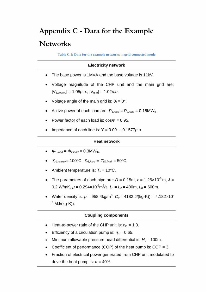
Appendix C - Data for the Example
Networks
Table C.1: Data for the example networks in grid-connected mode
Electricity network
· The base power is 1MVA and the base voltage is 11kV.
· Voltage magnitude of the CHP unit and the main grid are:
|V1,source| = 1.05p.u., |Vgrid| = 1.02p.u.
· Voltage angle of the main grid is: θ4 = 0°.
· Active power of each load are: P1,load = P2,load = 0.15MWe.
· Power factor of each load is: cosΦ = 0.95.
· Impedance of each line is: Y = 0.09 + j0.1577p.u.
Heat network
· Φ1,load = Φ2,load = 0.3MWth.
· Ts1,source = 100°C, To1,load = To2,load = 50°C.
· Ambient temperature is: Ta = 10°C.
· The parameters of each pipe are: D = 0.15m, ε = 1.25×10⁻³ m, λ =
0.2 W/mK, μ = 0.294×10⁻⁶m2/s. L1 = L2 = 400m, L3 = 600m.
· Water density is: ρ = 958.4kg/m3. Cp = 4182 J/(kg·K)) = 4.182×10-
3 MJ/(kg·K)).
Coupling components
· Heat-to-power ratio of the CHP unit is: cm = 1.3.
· Efficiency of a circulation pump is: ηp = 0.65.
· Minimum allowable pressure head differential is: Hc = 100m.
· Coefficient of performance (COP) of the heat pump is: COP = 3.
· Fraction of electrical power generated from CHP unit modulated to
drive the heat pump is: α = 40%.
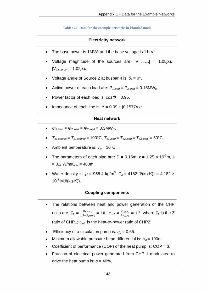
Appendix C - Data for the Example Networks
143
Table C.2: Data for the example networks in islanded mode
Electricity network
· The base power is 1MVA and the base voltage is 11kV.
· Voltage magnitude of the sources are: |V1,source| = 1.05p.u.,
|V2,source| = 1.02p.u.
· Voltage angle of Source 2 at busbar 4 is: θ4 = 0°.
· Active power of each load are: P1,load = P2,load = 0.15MWe.
· Power factor of each load is: cosΦ = 0.95.
· Impedance of each line is: Y = 0.09 + j0.1577p.u.
Heat network
· Φ1,load = Φ2,load = Φ2,load = 0.3MWth.
· Ts1,source = Ts1,source = 100°C, To1,load = To2,load = To3,load = 50°C.
· Ambient temperature is: Ta = 10°C.
· The parameters of each pipe are: D = 0.15m, ε = 1.25 × 10⁻³m, λ
= 0.2 W/mK, L = 400m.
· Water density is: ρ = 958.4 kg/m3. Cp = 4182 J/(kg·K)) = 4.182 ×
10-3 MJ/(kg·K)).
Coupling components
· The relations between heat and power generation of the CHP
units are:
,
, where is the Z
ratio of CHP1; is the heat-to-power ratio of CHP2.
· Efficiency of a circulation pump is: ηp = 0.65.
· Minimum allowable pressure head differential is: Hc = 100m.
· Coefficient of performance (COP) of the heat pump is: COP = 3.
· Fraction of electrical power generated from CHP 1 modulated to
drive the heat pump is: α = 40%.

Appendix D - Pipe Parameters for the Case Study
144
Appendix D - Pipe Parameters for the
Case Study Table D.1: Pipe Parameters for the Barry Island Case Study in Chapter 4
Pipe
No
From
node
To
node
Length
(m)
Diameter
(mm)
Heat transfer
coefficient
(W/mK)
Roughness
(mm)
01 01 02 257.6 125 0.321 0.4
02 02 03 97.5 40 0.21 0.4
03 02 04 51 40 0.21 0.4
04 02 05 59.5 100 0.327 0.4
05 05 06 271.3 32 0.189 0.4
06 05 07 235.4 65 0.236 0.4
07 07 08 177.3 40 0.21 0.4
08 07 09 102.8 40 0.21 0.4
09 07 10 247.7 40 0.21 0.4
10 05 11 160.8 100 0.327 0.4
11 11 12 129.1 40 0.21 0.4
12 11 13 186.1 100 0.327 0.4
13 13 14 136.2 80 0.278 0.4
14 14 15 41.8 50 0.219 0.4
15 15 16 116.8 32 0.189 0.4
16 15 17 136.4 32 0.189 0.4
17 14 18 136.4 32 0.189 0.4
18 14 19 44.9 80 0.278 0.4
19 19 20 136.4 32 0.189 0.4
20 19 21 134.1 32 0.189 0.4
21 19 22 41.7 65 0.236 0.4
22 22 23 161.1 32 0.189 0.4
23 22 24 134.2 32 0.189 0.4
24 22 25 52.1 65 0.236 0.4
25 25 26 136 32 0.189 0.4
26 25 27 123.3 32 0.189 0.4
27 25 28 61.8 40 0.21 0.4
28 28 29 95.2 32 0.189 0.4
29 28 30 105.1 32 0.189 0.4
30 31 28 70.6 125 0.321 0.4
31 31 7 261.8 125 0.321 0.4
32 32 11 201.3 125 0.321 0.4

Appendix E - Network Incidence Matrix for the Case Study
145
Appendix E - Network Incidence Matrix for the Case Study
1 2 3 4 5 6 7 8 9 10 11 12 13 14 15 16 17 18 19 20 21 22 23 24 25 26 27 28 29 30 31 32
1 -1
2 1 -1 -1 -1
3
1
4
1
5
1 -1 -1
-1
6
1
7
1 -1 -1 -1
1
8
1
9
1
10
1
11
1 -1 -1
12
1
13
1 -1
14
1 -1
-1 -1
15
1 -1 -1
16
1
17
1
18
1
19
1 -1 -1 -1
20
1
21
1
Table E.1: Network incidence matrix for the Barry Island district heating network case study
Pipe No. Pipe No.
Node
No.

Appendix E - Network Incidence Matrix for the Case Study
146
22
1 -1 -1 -1
23
1
24
1
25
1 -1 -1 -1
26
1
27
1
28
1 -1 -1 1
29
1
30
1
31
-1 -1
32
-1

Appendix F - Results Compared to SINCAL and IPSA for the Case Study
147
Appendix F - Results Compared to
SINCAL and IPSA for the Case Study
Table F.1: Temperatures and mass flow rates compared to SINCAL
Supply temperature Return temperature
Node
No.
Combined
analysis
SINCAL Combined
analysis
SINCAL
1 70 70 29.6314 29.6312
2 69.7533 69.7532 29.7125 29.7123
3 69.3054 69.3054 30 30
4 69.5787 69.5788 30 30
5 69.4764 69.4762 29.6517 29.6514
6 68.3920 68.3918 30 30
7 69.6565 69.6564 29.6881 29.6881
8 68.8555 68.8552 30 30
9 69.1869 69.1866 30 30
10 68.5491 68.5488 30 30
11 69.3902 69.3901 29.7259 29.7257
12 68.8090 68.8089 30 30
13 69.1844 69.1842 29.7243 29.7241
14 69.0567 69.0564 29.7669 29.7668
15 68.9284 68.9280 29.7738 29.7738
16 68.3118 68.3121 30 30
17 68.2110 68.2112 30 30
18 68.3362 68.3357 30 30
19 68.9764 68.9759 29.7605 29.7603
20 68.2575 68.2577 30 30
21 68.2693 68.2695 30 30
22 68.8315 68.8323 29.8015 29.8015
23 68.1949 68.1962 30 30
24 68.2992 68.3005 30 30
25 69.7547 69.7549 29.7795 29.7796
26 69.1947 69.1949 30 30
27 69.2461 69.2464 30 30
28 69.8821 69.8821 29.7956 29.7956
Mass flow rate
Pipe
No.
Combined
analysis
SINCAL
1 4.7982 4.7971
2 0.6509 0.6509
3 0.8760 0.8760
4 3.2712 3.2702
5 0.6664 0.6664
6 -0.8802 -0.8724
7 0.6585 0.6585
8 0.6529 0.6529
9 0.6637 0.6637
10 3.4849 3.4762
11 0.6593 0.6592
12 4.1925 4.1899
13 4.1925 4.1839
14 1.0062 1.0061
15 0.5024 0.5024
16 0.5038 0.5037
17 0.5021 0.5021
18 2.1914 2.189
19 0.5031 0.5031
20 0.5030 0.5029
21 1.1852 1.1830
22 0.6699 0.6698
23 0.6681 0.6679
24 -0.1527 0.1608
25 0.6528 0.6528
26 0.6519 0.6519
27 -1.4574 -1.4594
28 0.6480 0.6480

Appendix F - Results Compared to SINCAL and IPSA for the Case Study
148
29 69.4858 69.4858 30 30
30 69.4452 69.4452 30 30
31 70 70 29.6552 29.6554
32 70 70 29.5906 29.5905
29 0.6486 0.6486
30 2.7540 2.7560
31 3.5005 3.4987
32 2.2471 2.2471
Table F.2: Heat power compared to SINCAL
Heat power from Source 2 (heat slack)
Combined analysis SINCAL
0.8100 0.8099
Table F.3: Voltage magnitudes and angles compared to IPSA
Voltage magnitude Voltage angle
Busbar No. Combined analysis IPSA Combined analysis IPSA
1 1.0488 1.0488 -0.63 -0.63
2 1.0488 1.0488 -0.63 -0.63
3 1.0490 1.0490 -0.66 -0.66
4 1.0493 1.0493 -0.71 -0.71
5 1.0499 1.0499 -0.74 -0.75
6 1.0499 1.0499 -0.75 -0.74
7 1.05 1.05 -0.72 -0.72
8 1.05 1.05 -0.76 -0.76
9 1.02 1.02 0 0
Table F.4: Electrical power compared to IPSA
Electrical power from Source 1 (electrical slack)
Combined analysis IPSA
0.8118 0.8118